Minimal-size Real Space $d$ -wave Pairing Operator in CuO₂ Planes

Adriana Moreo Affiliation: Department of Physics and Astronomy,University of Tennessee, Knoxville, TN 37966, USA Elbio Dagotto Affiliation: Department of Physics and Astronomy,University of Tennessee, Knoxville, TN 37966, USA Affiliation: Materials Science and Technology Division, Oak Ridge National Laboratory,Oak Ridge, TN 37831, USA

August 11, 2026

Abstract

A novel minimal-size pairing operator $\Delta^{\dagger}_{D0}$ with $d$ -wave symmetry in CuO₂ planes is introduced. This pairing operator creates on-site Cooper pairs at the four oxygens that surround a copper atom. Via the time evolution of $\Delta^{\dagger}_{D0}$ , an additional inter-orbital pairing operator $\Delta^{\dagger}_{Dpd}$ with $d$ -wave symmetry is generated that pairs fermions located in a Cu and its four surrounding O’s. The subsequent time evolution of $\Delta^{\dagger}_{Dpd}$ generates an intra-orbital $d$ -wave pairing operator $\Delta^{\dagger}_{Dpp}$ involving the four O atoms that surround a Cu, as well as the $d$ -wave operator $\Delta^{\dagger}_{D}$ traditionally used in single-band models for cuprates. Because we recover the larger size operators extensively used in the three-orbital Hubbard model, we suggest that long-range order using the canonical extended operators occurs together with long-range order in the new minimal operators. However, our minimal $d$ -wave operators could be more practical to study $d$ -wave superconductivity because in the finite-size relatively small systems accessible to computational techniques it is easier to observe long-range order using local operators. Moreover, an effective model with the usual tight-binding hopping of the CuO₂ planes supplemented by an attractive potential $V$ in the $d$ -wave channel is introduced. Using mean-field techniques we show that a paired ground state is stabilized for any finite value of $V$ . We observed that the values of $V$ that lead to gap sizes similar to those in the cuprates are smaller for $d$ -wave pairing operators that include Cu $d$ -orbitals than those that only include $p$ -orbitals. In all cases the gap that opens in the spectrum has standard $d$ -wave symmetry. Finally, a simpler effective model is introduced to study the phenomenology of multi-orbital $d$ -wave superconductors, similarly as the negative- $U$ Hubbard model is used for properties of $s$ -wave superconductors.

pacs

74.72-h, 74.25.-q

I Introduction

The discovery of $d$ -wave superconductivity in the high critical temperature cuprates dwave1; dwave2 started efforts to develop effective Hamiltonians that would allow to study $d$ -wave pairing in the same way as the negative- $U$ Hubbard model allows the study of $s$ -wave pairing in standard BCS superconductors uneg1; uneg2; uneg3. Previous efforts focused on single-orbital systems with on-site Coulomb repulsion together with an effective attractive nearest-neighbors potential dw1; dw2, hardcore dimers dw3, or via the phenomenological addition of a term proportional to the square of the nearest-neighbor hoppings dw4. These models were difficult to study, parameters needed to be fine tuned, and actual numerical evidence of long-range $d$ -wave pairing correlations has been elusive dw3bis. The contribution of orbital degrees of freedom to the symmetry of the pairing operator came to the foreground when superconductivity was observed in iron-based pnictides and selenides fe1; fe2; fe3; fe4 and recently an effective model with on-site inter-orbital attraction was presented dw5. While relatively easy to study, inter-orbital same-site pairing operators are considered to be less likely to develop long-range order than their intra-orbital counterparts involving the same orbital but at different sites. For all these reasons, it is still important to find alternative and practical intra-orbital pairing operators with $d$ -wave symmetry.

In addition, recent angle-resolved photoemission experiments using Bi₂Sr₂CaCu₂O_8+δ indicated a novel “starfish” shape of the superconducting pairs with a very short length – of the order of one lattice space – in the antinodal direction smallpairs. This unexpected result appears to be doping independent and it may offer clues on the local structure of $d$ -wave pairs in the strong coupling regime. For us these experiments provide additional motivation to reconsider the local form of the $d$ -wave pairing operators in the cuprates.

Most previous attempts to construct same-orbital effective $d$ -wave models, analogous to the $U<0$ Hubbard model for $s$ -wave, relied on single-orbital systems with electrons placed on sites of a square lattice that mimic only the coppers. In the present publication, we aim to explore whether effective models for $d$ -wave superconductivity can be constructed using, instead, the oxygen locations in the more realistic CuO₂ lattice. It is well known that holes tend to reside on oxygens due to the charge transfer nature of the cuprates. However, the vast majority of theory efforts in this context rely on one-orbital Cu-only models, such as the $t-J$ and one-orbital Hubbard. Only recently computational efforts are studying the full CuO₂ models, with both Cu and O incorporated, and interesting results such as stripes have already been unveiled in this context sfermion2; p3b3; devereaux. Thus, our focus and main question addressed are timely: can we find an effective model for $d$ -wave superconductivity using only the oxygens of a CuO₂ lattice, namely only the atoms placed at the bonds of the said square lattice? Moreover, in searching for the most compact in size form for this pairing operator we will address, as a bonus, the recent photoemission results in the cuprates that unveiled very small Cooper pairs, at least in the antinodal directions smallpairs. Our overarching goal can be framed similarly as early studies within one-orbital models that attempted to construct quasiparticle operators with a larger quasiparticle weight $Z$ that those of the usual bare operators (i.e. better ”antennas”), and thus derive pairing operators that could produce stronger signals in computational studies sch-dag.

This paper is organized as follows: in Section II the models traditionally used to study the cuprates, as well as the $d$ -wave pairing operators previously investigated, are discussed. Our new minimal $d$ -wave pairing operator in the CuO₂ planes is introduced in Section III, while in Section IV additional $d$ -wave pairing operators, including the more standard extended ones, are deduced by calculating the time evolution of the minimal operator. Both the minimal and some extended pairing operators are studied at the mean-field level in Section V and a simple effective model is introduced in Section VI. Section VII is devoted to our conclusions.

II Models and Previously Used $d$ -wave Pairing Operators for Cuprates

It is widely accepted that a realistic model to describe CuO₂ planes is a three-orbital Hubbard model that includes the $d_{x^{2}-y^{2}}$ orbitals at the coppers and the $p_{\sigma}$ orbitals at the oxygens at a distance $\hat{\mu}/2$ from the coppers (lattice constant units), with $\hat{\mu}=x$ or $y$ emery i.e. along the two directions. The Hamiltonian is

H_{\rm 3BH}=H_{\rm TB}+H_{\rm int},

(1)

where

\begin{split}H_{\rm TB}=-t_{pd}\sum_{{\bf i},\mu,\sigma}\alpha_{{\bf i},\mu}(p^{\dagger}_{{\bf i}+{\hat{\mu}\over{2}},\mu,\sigma}d_{{\bf i},\sigma}+h.c.)-\\ t_{pp}\sum_{{\bf i},\langle\mu,\nu\rangle,\sigma}\alpha^{\prime}_{{\bf i},\mu,\nu}[p^{\dagger}_{{\bf i}+{\hat{\mu}\over{2}},\mu,\sigma}(p_{{\bf i}+{\hat{\nu}\over{2}},\nu,\sigma}+p_{{\bf i}-{\hat{\nu}\over{2}},\nu,\sigma})+h.c.]\\ +\epsilon_{d}\sum_{{\bf i}}n^{d}_{{\bf i}}+\epsilon_{p}\sum_{{\bf i},\mu}n^{p}_{{\bf i}+{\hat{\mu}\over{2}}}+\mu_{e}\sum_{{\bf i},\mu}(n^{p}_{{\bf i}+{\hat{\mu}\over{2}}}+n^{d}_{\bf i}),\end{split}

(2)

and

\begin{split}H_{\rm int}=U_{d}\sum_{{\bf i}}n^{d}_{\bf i,\uparrow}n^{d}_{\bf i,\downarrow}+U_{p}\sum_{{\bf i},\mu,\sigma}n^{p}_{{\bf i}+{\hat{\mu}\over{2}},\uparrow}n^{p}_{{\bf i}+{\hat{\mu}\over{2}},\downarrow}.\end{split}

(3)

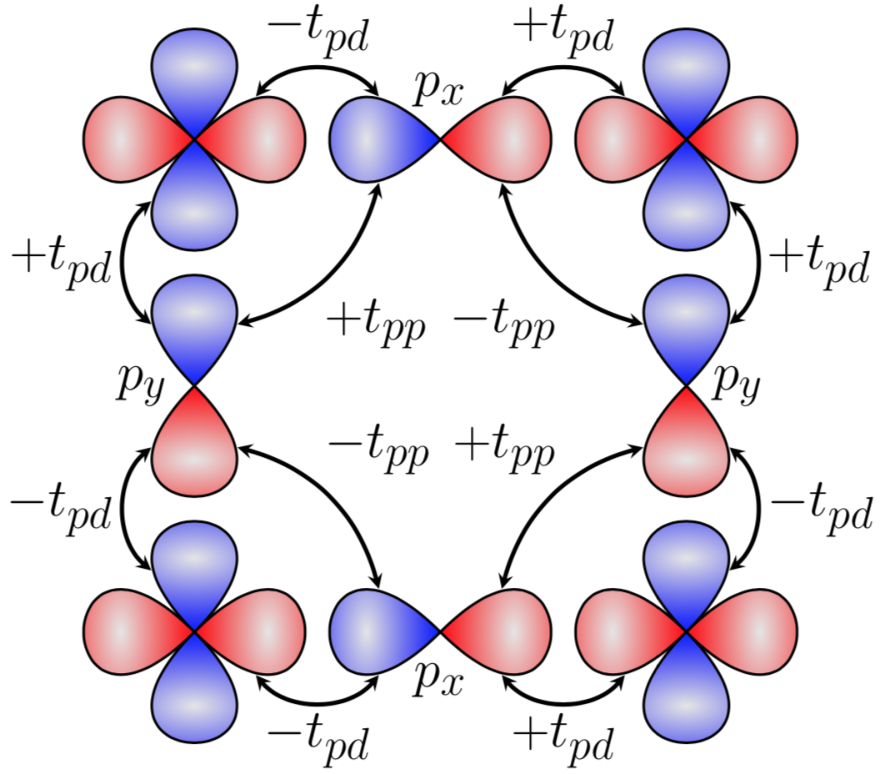
The operator $d^{\dagger}_{{\bf i},\sigma}$ creates an electron with spin $\sigma$ at site ${\bf i}$ of the copper square lattice, while $p^{\dagger}_{{\bf i}+{\hat{\mu}\over{2}},\mu,\sigma}$ creates an electron with spin $\sigma$ at orbital $p_{\mu}$ , where $\mu=x$ or $y$ , for the oxygen located at ${\bf i}+{\hat{\mu}\over{2}}$ . The hopping amplitudes $t_{pd}$ and $t_{pp}$ correspond to the hybridizations between nearest-neighbors Cu-O and O-O, respectively, and $\langle\mu,\nu\rangle$ indicate O-O pairs connected by $t_{pp}$ as shown in Fig. 1. $n^{p}_{{\bf i}+{\hat{\mu}\over{2}},\sigma}$ ( $n^{d}_{{\bf i},\sigma}$ ) is the number operator for $p$ ( $d$ ) electrons with spin $\sigma$ , and $\epsilon_{d}$ and $\epsilon_{p}$ are the on-site energies at the Cu and O sites, respectively. The Coulomb repulsion between two electrons at the same site and orbital is $U_{d}$ ( $U_{p}$ ) for $d$ ( $p$ ) orbitals. The signs of the Cu-O and O-O hoppings due to the symmetries of the orbitals is included in the parameters $\alpha_{{\bf i},\mu}$ and $\alpha^{\prime}_{{\bf i},\mu,\nu}$ and follow the convention shown in Fig. 1. Finally, $\mu_{e}$ is the electron chemical potential. The hopping parameters are those much used for the cuprates i.e. $t_{pd}=1.3$ eV and $t_{pp}=0.65$ eV, on-site energy $\epsilon_{p}=-3.6$ eV hybertsen, and $\Delta_{CT}=\epsilon_{d}-\epsilon_{p}$ which is positive ( $\epsilon_{d}=0$ ) sfermion1 is the charge-transfer gap.

Refer to caption — Figure 1: (color online) Schematic drawing of the Cu $d_{x^{2}-y^{2}}$ orbitals at the copper sites of the square lattice, with the sign convention indicated by the colors (red for + and blue for -). The oxygen $p_{\sigma}$ orbitals with their corresponding sign convention are also shown, located at the Cu-O-Cu bonds. The sign convention for the $t_{pd}$ and $t_{pp}$ hoppings is also presented.

II.1 Single-orbital $d$ -wave operators

Because experiments indicate that the Fermi surface of the cuprates is determined by a single band sb1; sb2; sb3; sb4, and theoretically a mapping of the three-band Hubbard model to the $t-J$ Hamiltonian can be obtained via Zhang-Rice singlets ZR, using only one band is appealing. In fact, due to their relative simplicity, the study of single-orbital models has prevailed in the cuprates. As a result, the simplest pairing operators with $d$ -wave symmetry are extended in the sense that they involve nearest-neighbor Cu sites elbioreview; Doug, without the oxygens in between. Zhang and Rice studied the addition of one hole in an undoped three-orbital Hubbard model using a CuO₄ cluster but neglecting the O-O hopping. They found that the hole occupies a symmetric linear combination involving the four O’s around a Cu, and forms a spin singlet together with the hole in the central Cu ZR. They also showed that the energy of the small cluster with two extra holes in the O orbitals was higher than the energy of two separated O holes. The next step was to construct Wannier functions combining the single-cluster symmetric single-hole plaquette states and obtain the effective single-orbital low-energy model, leading to the $t-J$ model. As discussed earlier, the simplest $d$ -wave pairing operator in the $t-J$ (and one-orbital Hubbard) modes involves nearest-neighbor sites and has the well-known form:

\Delta^{\dagger}_{D}({\bf j})=\sum_{\mu,\sigma}f(\sigma)\gamma_{\mu}c^{\dagger}_{{\bf j}+\hat{\mu},\sigma}c^{\dagger}_{{\bf j},-\sigma},

(4)

where $c^{\dagger}_{{\bf j},\sigma}$ creates an electron with spin $\sigma$ at site ${\bf j}$ of the Cu square lattice [see panel (a) of Fig. 2], $\gamma_{\mu}$ =1 (-1) for $\mu=\pm x$ ( $\pm y$ ) and $f(\sigma)=1(-1)$ if $\sigma=\uparrow(\downarrow)$ .

II.2 Three-orbital extended $d$ -wave operators

Note that the empty sites (holes) in the effective $t-J$ model contain Zhang-Rice singlets (ZRS) which means that the components of the Cooper pair in Eq. (4) are created on top of the ZRS. The first numerical calculations studying pairing were performed in single-orbital models elbioreview and when, later on, pairing was numerically evaluated in three-orbital Hubbard models, the pairing operators used p3b1; p3b2; p3b3 were straightforward generalizations of Eq. (4) [see panel (b) of Fig. 2] involving several sites, such as

\begin{split}\Delta^{\dagger}_{D3B}({\bf j})=\sum_{\mu,\sigma}f(\sigma)\gamma_{\mu}[d^{\dagger}_{{\bf j}+\hat{\mu},\sigma}d^{\dagger}_{{\bf j},-\sigma}+\\ p^{\dagger}_{{\bf j}+\hat{\mu}+x/2,x,\sigma}p^{\dagger}_{{\bf j}+x/2,x,-\sigma}+\\ p^{\dagger}_{{\bf j}+\hat{\mu}+y/2,y,\sigma}p^{\dagger}_{{\bf j}+y/2,y,-\sigma}].\end{split}

(5)

This operator creates electrons that form intra-orbital pairs whose $d$ -wave symmetry is determined by $\gamma_{\mu}$ . It considers that Cooper pairs are formed by one electron (or hole) in a Cu and another in its neighboring Cu atoms, and similarly for electrons (or holes) in the $p$ -orbitals. It is in this sense that this operator is intra-orbital: the pair terms involve either Cu or O. In real space the minimum pair created by the pairing operators in Eqs. 4 and 5 involves five lattice sites, in a single-orbital model context, or several unit cells (21 Cu and O sites) for the three-orbital case. Such extended pairing operators [see panels (a) and (b) of Fig. 2] appear at odds with the recent experimental results of Ref. smallpairs where the observed pairs have a minimum real-space extension of the order of the lattice constant along the antinodal direction. This photoemission experiment offers motivation to investigate if in the CuO₂ planes it is possible to construct a more local $d$ -wave pairing operator involving far less sites and ideally just one unit cell.

Figure 2: (color online) Schematic drawing of previously used

d

-wave pairing operators in the CuO₂ planes. Circles indicate the Cu

d

-orbitals sites while red (blue) squares indicate the O

p_{\rm x}

(

p_{\rm y}

) orbitals sites. Filled symbols indicate atoms where the particles forming the Cooper pairs are located and arrows indicate the spin of the electrons/holes in the pair. (a) In single-orbital approximations to the CuO₂ planes the Cooper pairs are assumed to be primarily located in nearest-neighbor Cu sites via the operator

\Delta^{\dagger}_{D}

. (b) In the three-orbital Hubbard model the

d

-wave pairing operator

\Delta^{\dagger}_{D3B}

adds Cooper-pairs involving

p_{\rm x}

and

p_{\rm y}

orbitals, in addition to the Cu orbitals as in (a) not shown in this panel for clarity. The individual Cooper pairs are encircled with ellipses. The relative phases are positive along

x

and negative along

y

III Minimal $d$ -wave pairing operator

As explained, in undoped systems and in the Zhang-Rice approximation a doped hole is placed at an oxygen and forms a ZRS with the hole at a copper. A second doped hole is expected to form another ZRS with a different Cu. The one-orbital pairing operator in Eq. (4) can only involve electrons at two neighboring Cu sites, each with its own ZRS. However, in the three-orbital Hubbard model formulation there is no clear relation between the pairing operator and the two neighboring ZRS. Equation (5) just considers that the minimal Cooper pair can be formed by fermions at a $d$ ( $p_{\sigma}$ ) orbital and at the four nearest-neighbor Cu (O) atoms, thus involving five unit cells, and many sites.

As discussed above, Zhang and Rice found out that it would be unlikely that two holes would share the O orbitals of one single plaquette. However, calculations including $t_{pp}$ hopping and the $p-d$ Coulomb repulsion, both neglected in the ZRS derivation, indicated that an effective attraction between holes in the oxygens of a single plaquette may develop varma; cristian. Thus, the possibility that two holes could form a pair in the O orbitals in a single plaquette deserves to be explored.

First, we will construct an on-site $d$ -wave pairing operator which considers only doubly occupied O sites [see panel (a) in Fig. 3] in analogy with the on-site attractive $s$ -wave pairing operator. It has the form

\begin{split}\Delta^{\dagger}_{D0}({\bf j})={1\over{2}}\sum_{\mu,\sigma}f(\sigma)\gamma_{\mu}p^{\dagger}_{{\bf j}+\hat{\mu}/2,\mu,\sigma}p^{\dagger}_{{\bf j}+\hat{\mu}/2,\mu,-\sigma}=\\ \sum_{\mu}\gamma_{\mu}p^{\dagger}_{{\bf j}+\hat{\mu}/2,\mu,\uparrow}p^{\dagger}_{{\bf j}+\hat{\mu}/2,\mu,\downarrow}.\end{split}

(6)

Although the operator involves doubly-occupied sites, each one apparently $s$ -wave, since the operator involves four oxygens around the same copper, a linear combination can be made that renders the full operator $d$ -wave.

Figure 3: (color online) Schematic drawing of the minimal intra-unit cell

d

-wave pairing operators introduced here for the CuO₂ planes, that were not explored before in three-orbital Hubbard models to our knowledge. Circles indicate the Cu

d

-orbitals while the red (blue) squares indicate the

p_{\rm x}

(

p_{\rm y}

) orbitals at the O atoms. Filled symbols indicate sites where the particles forming the Cooper pairs are located and arrows indicate the spin of the electrons/holes in the pair. (a) On-site intra-orbital (i.e. same oxygen)

d

-wave operator

\Delta^{\dagger}_{D0}

, defined in Eq. (6). Here the two members of the Cooper pair are at the same oxygen, linearly combined involving the four possible oxygens. (b) More extended nearest-neighbor intra-orbital

d

-wave operator

\Delta^{\dagger}_{Dpp}

where the Cooper pair is formed by two electrons in the same

p_{\sigma}

orbital, either

x

y

, at a distance of one lattice spacing forming a spin singlet, and linearly combining the vertical and horizontal directions to form a

d

-wave operator. (c) Inter-orbital (

dp

)

d

-wave operator

\Delta^{\dagger}_{Dpd}

with pairs involving a particle at the central Cu and the other at a neighboring O, linearly combined to form a

d

-wave. (d) Plaquette

d

-wave intraorbital pairing operator

\Delta^{\dagger}_{Dplaq}

in the CuO₂ plane. In (a-d), the Cooper pairs are encircled with ellipses. Relative phases are positive along

x

and negative along

y

, leading to a

d

-wave.

IV Time-Evolution of the pairing operator

In previous literature zhang; you a relationship between the on-site and the extended $s$ -wave pairing operators in the single-orbital Hubbard model was obtained by calculating the time evolution of the on-site pairing operator. Following similar steps we can now calculate the time evolution of the on-site minimal $d$ -wave pairing operator $\Delta^{\dagger}_{D0}$ proposed in Eq. (6) for the three-orbital Hubbard model Eq. (1). We found that

\begin{split}-i{d\Delta^{\dagger}_{D0}\over{dt}}=[H_{3BH},\Delta^{\dagger}_{D0}]=\\ 2(\epsilon_{p}-\mu_{e})\Delta^{\dagger}_{D0}-U_{p}\Delta^{\dagger}_{D0}-t_{pd}\Delta^{\dagger}_{Dpd},\end{split}

(7)

where $\Delta^{\dagger}_{Dpd}$ is another $d$ -wave pairing operator defined in one unit-cell CuO₂. $\Delta^{\dagger}_{Dpd}$ forms Cooper pairs with one fermion at a Cu and the other in an antisymmetric linear combination of the p_σ orbitals in its four nearest-neighboring O’s [panel (c) of Fig. 3] and it is given by

\Delta^{\dagger}_{Dpd}({\bf j})=\sum_{\mu,\sigma}f_{\sigma}\gamma_{\mu}\alpha_{{\bf j},\mu}d^{\dagger}_{{\bf j},\sigma}p^{\dagger}_{{\bf j}+\hat{\mu}/2,\mu,-\sigma}.

(8)

Since in the ground state the average value of the pairing operators is time-independent, from Eq. (7) we see that the average values of the two pairing operators must be related. In addition, by evaluating the time evolution of the new inter-orbital minimal pairing operator, $\Delta^{\dagger}_{Dpd}$ , more extended intra- and inter-orbital pairing operators with $d$ -wave symmetry are obtained. For example, from the commutator between $\Delta^{\dagger}_{Dpd}$ and the $t_{pd}$ hopping term in $H_{\rm 3BH}$ we obtain the nearest-neighbor $d$ -orbital pairing operator in Eq. (4) depicted in panel (a) of Fig. 2 and an additional intra-orbital pairing operator given by

\begin{split}\Delta^{\dagger}_{Dpp}({\bf j})=(p^{\dagger}_{{\bf j}+x/2,x,\uparrow}p^{\dagger}_{{\bf j}-x/2,x,\downarrow}-p^{\dagger}_{{\bf j}+x/2,x,\downarrow}p^{\dagger}_{{\bf j}-x/2,x,\uparrow})-\\ (p^{\dagger}_{{\bf j}+y/2,y,\uparrow}p^{\dagger}_{{\bf j}-y/2,y,\downarrow}-p^{\dagger}_{{\bf j}+y/2,y,\downarrow}p^{\dagger}_{{\bf j}-y/2,y,\uparrow})=\\ \sum_{\mu,\sigma}f_{\sigma}\gamma_{\mu}p^{\dagger}_{{\bf j}+\hat{\mu}/2,\mu,\sigma}p^{\dagger}_{{\bf j}-\hat{\mu}/2,\mu,-\sigma},\end{split}

(9)

which is another $B_{1g}$ intra-orbital pairing operator with the two particles located in the same orbital but at different oxygens [see panel (b) in Fig. 3] and it is analogous to the extended, nearest-neighbor, $s$ -wave operator defined in the context of the cuprates elbioreview; zhang. In addition, the commutator between $\Delta^{\dagger}_{Dpd}$ and the $t_{pp}$ hopping term in $H_{\rm 3BH}$ leads to an extended version of $\Delta^{\dagger}_{Dpd}$ that forms pairs with one fermion on a $d$ orbital at site ${\bf r}$ and the other at orbital $p_{x}$ ( $p_{y}$ ) at distance ${\bf r}+y+x/2$ ( ${\bf r}+x+y/2$ ) and symmetrical points. The commutator of this extended operator with the $t_{pd}$ hopping term in $H_{\rm 3BH}$ finally leads to $p$ -orbital pairing operators that combine fermions in $p_{\rm x}$ ( $p_{\rm y}$ ) orbitals along the $y$ ( $x$ ) direction which are the plaquette pairing operators mentioned in Ref. smallpairs and shown in panel (d) of Fig. 3. They are given by

\begin{split}\Delta^{\dagger}_{Dplaq}({\bf j})=(p^{\dagger}_{{\bf j}+x/2,x,\uparrow}p^{\dagger}_{{\bf j}+y+x/2,x,\downarrow}-\\ p^{\dagger}_{{\bf j}+x/2,x,\downarrow}p^{\dagger}_{{\bf j}+y+x/2,x,\uparrow})-\\ (p^{\dagger}_{{\bf j}+y/2,y,\uparrow}p^{\dagger}_{{\bf j}+x+y/2,y,\downarrow}-\\ p^{\dagger}_{{\bf j}+y/2,y,\downarrow}p^{\dagger}_{{\bf j}+x+y/2,y,\uparrow})=\\ \sum_{\mu,\sigma}f_{\sigma}\gamma_{\mu}p^{\dagger}_{{\bf j}+\hat{\mu}/2,\mu,\sigma}p^{\dagger}_{{\bf j}+\bar{\mu}+\hat{\mu}/2,\mu,-\sigma},\end{split}

(10)

where $\bar{\mu}=x$ ( $y$ ) if $\mu=y$ ( $x$ ). We also notice that the $p$ contribution in the standard $d$ -wave pairing operator in Eq. (5) results from a combination of the intra-orbital $p$ pairing operators operators $\Delta^{\dagger}_{Dplaq}$ and $\Delta^{\dagger}_{Dpp}$ .

The relationships between the minimal and the compact, but more extended, $d$ -wave pairing operators in Fig. 3 deduced from the time-evolution calculations suggest that if the Hamiltonian indeed has a superconducting ground state with $d$ -wave symmetry we would expect that $all$ the pairing operators with that symmetry will develop long-range order simultaneously. In practice we expect the long-range behavior of local operators to be easier to study in the finite, often small, clusters accessible to numerical studies. For this reason, we will focus on the newly introduced $d$ -wave pairing operators shown in Fig. 3 and we will compare them with the traditional ones presented in Fig. 2.

V Effective model for $d$ -wave pairing

To show explicitly that the pairing operators in Eq. (6), Eq. (8), Eq. (9), and Eq. (10) indeed lead to $d$ -wave superconductors we will study the phenomenological Hamiltonian given by

H_{\rm 3BDW}=H_{\rm TB}+H_{\rm int},

(11)

where the tight-binding term is the canonical of the three-orbital Hubbard model for cuprates [Eq. (2)] and the interacting portion of the Hamiltonian for the on-site same-oxygen pairing, as in $D_{0}$ , is given by

\begin{split}H^{(0)}_{\rm int}=-\sum_{{\bf j},\mu,\sigma}\gamma_{\mu}f(\sigma)[p^{\dagger}_{{\bf j}+\hat{\mu}/2,\mu,\sigma}p^{\dagger}_{{\bf j}+\hat{\mu}/2,\mu,-\sigma}\Delta+\\ \Delta^{*}p_{{\bf j}-\hat{\mu}/2,\mu,-\sigma}p_{{\bf j}-\hat{\mu}/2,\mu,\sigma}].\end{split}

(12)

$\Delta$ and $\Delta^{*}$ are parameters that determine the strength of the superconducting condensate and they contain also the attractive coupling $V$ usually employed in these phenomenological models. For the case of the inter-orbital extended pairing $\Delta^{\dagger}_{Dpd}$ the interaction term is given by

\begin{split}H^{(pd)}_{\rm int}=-\sum_{{\bf j},\mu,\sigma}\gamma_{\mu}f(\sigma)\alpha_{{\bf j},\mu}[d^{\dagger}_{{\bf j},\sigma}p^{\dagger}_{{\bf j}-\mu/2,\mu,-\sigma}\Delta+\\ \Delta^{*}p_{{\bf j}-\mu/2,\mu,-\sigma}d_{{\bf j},\sigma}].\end{split}

(13)

For the intra-orbital extended pairing $\Delta^{\dagger}_{Dpp}$ the interaction term is given by

\begin{split}H^{(pp)}_{\rm int}=-\sum_{{\bf j},\mu,\sigma}\gamma_{\mu}f(\sigma)[p^{\dagger}_{{\bf j}+\hat{\mu}/2,\mu,\sigma}p^{\dagger}_{{\bf j}-\hat{\mu}/2,\mu,-\sigma}\Delta+\\ \Delta^{*}p_{{\bf j}-\hat{\mu}/2,\mu,-\sigma}p_{{\bf j}+\hat{\mu}/2,\mu,\sigma}],\end{split}

(14)

while for the plaquette operator $\Delta^{\dagger}_{Dplaq}$ the interaction is given by

\begin{split}H^{(plaq)}_{\rm int}=-\sum_{{\bf j},\mu,\sigma}\gamma_{\mu}f(\sigma)[p^{\dagger}_{{\bf j}+\hat{\mu}/2,\bar{\mu},\sigma}p^{\dagger}_{{\bf j}-\hat{\mu}/2,\bar{\mu},-\sigma}\Delta+\\ \Delta^{*}p_{{\bf j}-\hat{\mu}/2,\bar{\mu},-\sigma}p_{{\bf j}+\hat{\mu}/2,\bar{\mu},\sigma}].\end{split}

(15)

V.1 Mean-Field analysis

In this section we perfom a canonical mean-field analysis of the effective pairing models now using the more compact $d$ -wave operators introduced here. As usual, via a Fourier transform we can work in momentum space which is more convenient. Thus, $H_{\rm TB}$ can be written as

H_{\rm TB}({\bf k})=\sum_{{\bf k},\sigma}\Phi^{\dagger}_{{\bf k},\sigma}\xi_{{\bf k}}\Phi_{{\bf k},\sigma},

(16)

where $\Phi^{\dagger}_{{\bf k},\sigma}=(p^{\dagger}_{x}({\bf k}),p^{\dagger}_{y}({\bf k}),d^{\dagger}({\bf k}))_{\sigma}$ and

\xi_{\bf k}=\left(\begin{array}[]{ccc}\epsilon_{p}&-4t_{pp}s_{x}s_{y}&-2it_{pd}s_{x}\\ -4t_{pp}s_{x}s_{y}&\epsilon_{p}&-2it_{pd}s_{y}\\ 2it_{pd}s_{x}&2it_{pd}s_{y}&0\end{array}\right),

(17)

where $s_{i}$ indicates $\sin(k_{i}/2)$ with $i=x$ or $y$ .

Note that in the electron representation the undoped case is characterized by one hole at the Cu and no holes at the O, which corresponds to a total of five electrons per CuO₂ unit-cell (the maximum possible electronic number in three orbitals is six). The orbital-resolved tight-binding bands along the $\Gamma-X-M-\Gamma$ path in the Brillouin zone calculated using a $100\times 100$ square lattice (with Cu’s at the sites of the lattice) is in Fig. 4. The dashed black line is the chemical potential $\mu_{e}$ for the important electronic density $\langle n\rangle=5$ and the corresponding Fermi surface is in the inset. An analysis of the orbital composition of each of the three bands, shown by the color palette in the figure, indicates that the top band is purely $d$ at the $\Gamma$ point and moving away from $\Gamma$ becomes hybridized with the $p$ orbitals such that its $d$ content becomes 78% at X and 56% at M. The two bottom bands have pure $p$ character at the Brillouin zone center. The middle band achieves 43% $d$ character at M, while the lower band has 21% $d$ character at X. Note that the tight-binding Fermi surface, shown in the inset, has the qualitative form expected in the cuprates, both from the theory and experimental perspectives. However, its orbital content is only about 75% $d$ in average, showing that the oxygen component is not negligible even if only one band crosses the Fermi level.

Figure 4: (color online) Band dispersion for the tight-binding term of the CuO₂ Hamiltonian. The orbital content is displayed with red (blue) indicating

d

(

p

) character. The dashed line indicates the position of the chemical potential (or Fermi level E_F) at density

\langle n\rangle=5

(undoped case). The Fermi surface at this density is in the inset. Colors indicate the orbital content of the bands, with the palette on the right denoting the weight of the

d

component (e.g. 1 means 100% copper

d

, and the oxygen weight is simply one minus the copper weight).

Note that $\xi_{\bf k}$ can be written in terms of the $3\times 3$ Gell’mann matrices schiff $\lambda_{i}$ for the cases $i=1$ to 8, while $\lambda_{0}$ is the $3\times 3$ identity (see Appendix for an explicit form of these matrices). This is useful in order to highlight the symmetry of its different terms:

\xi_{{\bf k}}={2\over{3}}\epsilon_{p}\lambda_{0}+{\sqrt{3}\over{3}}\epsilon_{p}\lambda_{8}+2t_{dp}(s_{x}\lambda_{5}+s_{y}\lambda_{7})-4t_{pp}s_{x}s_{y}\lambda_{1}.

(18)

Since the CuO₂ planes transform as $D_{\rm 4h}$ and the Hamiltonian has to be invariant under the group operations, i.e., it has to transform as the $A_{1g}$ representation of the group, we notice that in Eq. (18), $\lambda_{0}$ and $\lambda_{8}$ transform like $A_{1g}$ while $\lambda_{1}$ transforms like $B_{2g}$ , and $(\lambda_{5},\lambda_{7})$ transform like the two-dimensional representation $E_{g}$ since they are combined with $(s_{x},s_{y})$ , which transforms according to $E_{g}$ .

The interacting term of the Hamiltonian can be written in terms of a pairing matrix $P^{(0)}$ for the on-site same-oxygen case (Eq. (12)):

P^{(0)}_{\bf k}=\left(\begin{array}[]{ccc}2\Delta&0&0\\ 0&-2\Delta&0\\ 0&0&0\end{array}\right),

(19)

References

- (1) C. C. Tsuei, J. R. Kirtley, C. C. Chi, Lock See Yu-Jahnes, A. Gupta, T. Shaw, J. Z. Sun, and M. B. Ketchen, Phys. Rev. Lett. 73, 593 (1994).
- (2) J. R. Kirtley, C. C. Tsuei, J. Z. Sun, C. C. Chi, L. S. Yu-Jahnes, A. Gupta, M. Rupp, and M. B. Ketchen, Nature (London) 373, 225 (1995).
- (3) R. T. Scalettar, E. Y. Loh, J. E. Gubernatis, A. Moreo, S. R. White, D. J. Scalapino, R. L. Sugar, and E. Dagotto, Phys. Rev. Lett. 62, 1407 (1989).
- (4) A. Moreo and D. J. Scalapino, Phys. Rev. Lett. 66, 946 (1991).
- (5) M. Randeria, N. Trivedi, A. Moreo, and R. T. Scalettar, Phys. Rev. Lett. 69, 2001 (1992).
- (6) E. Dagotto, J. Riera, Y. C. Chen, A. Moreo, A. Nazarenko, F. Alcaraz, and F. Ortolani, Phys. Rev. B 49, 3548 (1994).
- (7) A. Nazarenko, A. Moreo, E. Dagotto, and J. Riera, Phys. Rev. B 54, R768 (1996).
- (8) D. S. Rokhsar and S. A. Kivelson, Phys. Rev. Lett. 61, 2376 (1988).
- (9) F. F. Assaad, M. Imada, and D. J. Scalapino, Phys. Rev. Lett. 77, 4592 (1996).
- (10) Phenomenologically, the coupling of fermions with classical pairing fields leads to -wave pairing, see M. Mayr, G. Alvarez, C. Sen, and E. Dagotto, Phys. Rev. Lett. 94, 217001 (2005), but we are searching for purely fermionic systems.
- (11) D. C. Johnston, Adv. Phys. 59, 803 (2010).
- (12) P. Dai, J. P. Hu, and E. Dagotto, Nat. Phys. 8, 709 (2012).
- (13) Y. Wan and Q.-H. Wang, Europhys. Lett. 85, 57007 (2009).
- (14) M. Daghofer, A. Moreo, J. A. Riera, E. Arrigoni, D. J. Scalapino, and E. Dagotto, Phys. Rev. Lett. 101, 237004 (2008).
- (15) C. B. Bishop, G. Liu, E. Dagotto, and A. Moreo, Phys. Rev. B 93, 224519 (2016).
- (16) H. Li, X. Zhou, S. Parham, K. N. Gordon, R. D. Zhong, J. Schneeloch, G. D. Gu, Y. Huang, H. Berger, G. B. Arnold, and D. S. Dessau, arXiv:1809.02194.
- (17) M. S. D. A. Hussein, E. Dagotto, and A. Moreo, Phys. Rev. B 99, 110158 (2019).
- (18) E. Arrigoni, M. Aichhorn, M. Daghofer, and W. Hanke, New J. Phys.11, 055066 (2009).
- (19) E. W. Huang, C. B. Mendl, S. Liu, S. Johnston, H-C. Jiang, B. Moritz, and T. P. Devereaux, Science 358, 1161 (2017).
- (20) E. Dagotto and J. R. Schrieffer, Phys. Rev. B 43 (RC), 8705 (1991).
- (21) V. J. Emery and G. Reiter, Phys. Rev. B 38, 11938(R) (1988).
- (22) M. S. Hybertsen, M. Schlüter, and N. E. Christensen, Phys. Rev. B 39, 9028 (1989).
- (23) M. S. D. A. Hussein, M. Daghofer, E. Dagotto, and A. Moreo, Phys. Rev. B 98, 035124 (2018).
- (24) Z.-X. Shen, J. W. Allen, J. J. Yeh, J.-S. Kang, W. Ellis, W. Spicer, I. Lindau, M. B. Maple, Y. D. Dalichaouch, M. S. Torikachvili, J. Z. Sun, and T. H. Geballe, Phys. Rev. B 36, 8414 (1987).
- (25) J. W. Allen, C. G. Olson, M. B. Maple, J.-S. Kang, L. Z. Liu, J.-H. Park, R. O. Anderson, W. P. Ellis, J. T. Markert, Y. Dalichaouch, and R. Liu, Phys. Rev. Lett. 64, 595 (1990).
- (26) B. O. Wells, Z.-X. Shen, A. Matsuura, D. M. King, M. A. Kastner, M. Greven, and R. J. Birgeneau, Phys. Rev. Lett. 74, 964 (1995).
- (27) A. Damascelli, Z. Hussain, and Z.-X. Shen, Rev. Mod. Phys. 75, 473 (2003).
- (28) F. C. Zhang and T. M. Rice, Phys. Rev. B 37, 3759 (1988).
- (29) E. Dagotto, Rev. Mod. Phys. 66, 763 (1994).
- (30) D. J. Scalapino, Phys. Reports 250, 329 (1995).
- (31) G. Dopf, A. Muramatsu, and W. Hanke, Phys. Rev. B 41, 9264 (1990).
- (32) Z. B. Huang, H. Q. Lin, and J. E. Gubernatis, Phys. Rev. B 63, 115112 (2001).
- (33) P. B. Littlewood and C. M. Varma, Phys. Rev. Lett. 63, 2602 (1989).
- (34) C. D. Batista and A. A. Aligia, Phys. Rev. B 48, 4212(R) (1993).
- (35) S. Zhang, Phys. Rev. B 42, 1012(R) (1990).
- (36) W-L. You, S-J. Gu, G-S. Tian, and H-Q. Lin, Phys. Rev. B 79, 014508 (2009).
- (37) L. Schiff, Quantum Mechanics, third ed. (McGraw-Hill Kogakusha, Tokyo, 1968).
- (38) M. Daghofer, A. Nicholson, A. Moreo, and E. Dagotto. Phys. Rev. B 81, 014511 (2010).
- (39) T. Yoshida1, M. Hashimoto, I. M. Vishik, Z-X. Shen, and A. Fujimori, J. Phys. Soc. Jpn. 81, 011006 (2012).
- (40) J.G. Zaanen, G.A. Sawatzky, and J.W. Allen, Phys. Rev. Lett. 55, 418 (1985).
- (41) While in BCS superconductors an infinitesimal attraction stabilizes the superconducting state, this may not be the case in the cuprates and, in addition, when the Coulomb interaction is taken into account the orbital content at the chemical potential for a doped system will contain more contributions than in the non-interacting case.