Right-handed Sterile neutrinos are elegantly embedded in the seesaw model. In type-I seesaw model the SM is extended by at least two heavy Sterile neutrino singlets $\nu_{\text{\tiny{R}}}^{i}$ ($i$ indicates the generation) with the following most general electroweak Lagrangian

$$\mathcal{L}=\mathcal{L}_{\text{\tiny{SM}}}+y_{ij}^{\nu}\bar{\ell}_{\text{\tiny{L}}}^{i}\tilde{H}\nu_{\text{\tiny{R}}}^{j}+\frac{1}{2}M_{\text{\tiny{R}}}^{i}\bar{\nu_{\text{\tiny{R}}}^{ic}}\nu_{\text{\tiny{R}}}^{i}+h.c.,$$

(1)

where $\mathcal{L}_{\text{\tiny{SM}}}$ denotes the electroweak Lagrangian of the SM and $y_{ij}^{\nu}$ is a matrix of Yukawa interactions, $H$ is the Higgs doublet and $\tilde{H}=\epsilon\,H^{*}$, with $\epsilon$ is the anti-symmetric SU(2)-invariant tensor, $\ell_{\text{\tiny{L}}}=(\nu_{\text{\tiny{L}}},e_{\text{\tiny{L}}})^{T}$ indicates the left handed lepton doublets and $\nu_{\text{\tiny{R}}}^{ic}=C\,\bar{\nu_{\text{\tiny{R}}}}^{iT}$ with $C=i\gamma_{2}\gamma_{0}$. Furthermore, $\nu^{i}_{\text{\tiny{R}}}$’s are SM gauge singlets, hence the Majorana mass term $M^{i}_{\text{\tiny{R}}}$ is allowed in addition to the Dirac mass $m_{\text{\tiny{D}}}$. Consequently, after the electroweak symmetry breaking one can obtain the Dirac mass as $m_{\text{\tiny{D}}}=y^{\nu}\left\langle H\right\rangle$ where by considering both Dirac and Majorana masses leads to the neutrino mass matrix as follows

$\displaystyle\mathcal{M}_{\nu}=\left(\begin{tabular}[]{c c}$0$&$m_{\text{\tiny{D}}}$\\ $m_{\text{\tiny{D}}}^{\text{\tiny{T}}}$&$M_{\text{\tiny{R}}}$\end{tabular}\right),$

where $M_{\text{\tiny{R}}}$ and $m_{\text{\tiny{D}}}$ are $3\times 3$ matrices. However, the eigenvalues of $M_{\text{\tiny{R}}}$ can be chosen to be at a scale much higher than the electroweak scale suppressing the Dirac mass term. Meanwhile, to diagonalize the mass matrix, one needs a $6\times 6$ mixing unitary matrix. In fact, the diagonalizing process occurs through two steps I) block diagonalizing and II) two unitary rotations. Therefore, there would be two sets of physical eigenstates related to the three light neutrinos of the SM particles. In the first set of eigenstates which are known as active neutrinos, the masses can be obtained as

$$m_{\nu}=-m_{\text{\tiny{D}}}^{\text{\tiny{T}}}\,M_{\text{\tiny{M}}}^{\tiny{-1}}m_{\text{\tiny{D}}},$$

(5)

and the neutrinos belong to the $SU(2)$ doublets. In the second set, one has a set of heavy right handed Majorana neutrinos which are gauge singlets with mass $M_{\text{\tiny{M}}}$ the eigenvalues of $M_{\text{\tiny{R}}}$. The scale of $M_{\text{\tiny{M}}}$ is not determined by experiment and different constraints are available from particle physics, astrophysics and cosmology with different consequences [49]. As a result, Sterile and the SM neutrinos mix with $\theta\equiv m_{\text{\tiny{D}}}M^{-1}_{\text{\tiny{M}}}$ mixing angle. Therefore, all of the Majorana mass eigenstates can be represented by the flavor vector elements as:

$\displaystyle N=V^{\dagger}_{\text{\tiny{N}}}\nu_{\text{\tiny{R}}}+\Theta^{\text{\tiny{T}}}\nu^{c}_{\text{\tiny{L}}}+h.c.\,,~~~~\text{and}~~~~\upnu=V^{\dagger}_{\nu}\nu_{\text{\tiny{L}}}-U^{\dagger}_{\nu}\theta\nu_{\text{\tiny{R}}}^{c}+h.c.\,,$

(6)

where $V_{\nu}$ is the usual neutrino mixing matrix connecting the observed light mass eigenstates $\nu_{i}$ to the active flavor eigenstates:

$$V_{\nu}\equiv(1-\frac{1}{2}\theta\theta^{\dagger})U_{\nu},$$

(7)

and $U_{\nu}$ is the unitary part of neutrino mixing matrix. Meanwhile, the corresponding parameters in the Sterile sector are $V_{\text{\tiny{N}}}$ and $U_{\text{\tiny{N}}}$ and the active-Sterile mixing angle is

$$\Theta\equiv\theta U_{\text{\tiny{N}}}^{\star}.$$

(8)

Thus the Sterile neutrinos interacts with the SM particles as follows

	$\displaystyle\mathcal{L}$	$\displaystyle\supset$	$\displaystyle\,\,\sum_{l}-\frac{g}{\sqrt{2}}\bar{N}\,\Theta^{\dagger}\,\gamma^{\mu}\,l_{\text{\tiny{L}}}\,W_{\mu}^{+}\,-\sum_{l}\frac{g}{\sqrt{2}}\,\bar{l}_{\text{\tiny{L}}}\,\gamma^{\mu}\,\Theta\,N\,W_{\mu}^{-}-\frac{g}{2\cos\theta_{\text{\tiny{W}}}}\,\bar{N}\,\Theta^{\dagger}\,\gamma^{\mu}\,\nu_{l_{\text{\tiny{L}}}}\,Z_{\mu}\,$		(9)
			$\displaystyle-\frac{g}{2\cos\theta_{\text{\tiny{W}}}}\,\bar{\nu}_{l_{\text{\tiny{L}}}}\,\gamma^{\mu}\,\Theta\,N\,Z_{\mu}-\frac{g}{\sqrt{2}}\,\frac{M_{\text{\tiny{N}}}}{m_{\text{\tiny{W}}}}\,\Theta\,h\,\bar{\nu}_{l_{\text{\tiny{L}}}}\,N\,-\frac{g}{\sqrt{2}}\,\frac{M_{\text{\tiny{N}}}}{m_{\text{\tiny{W}}}}\,\Theta^{\dagger}\,h\,\bar{N}\,\nu_{l_{\text{\tiny{L}}}}.$

where $l=e,\mu,\tau$ and $\nu_{l}$ denotes the left handed SM neutrinos in the flavor eigenstates which can be expressed in terms of the mass eigenstates as $\nu_{l_{\text{\tiny{L}}}}=P_{\text{\tiny{L}}}(V_{\nu}\upnu+\Theta N)$. However, a neutral and massive Sterile neutrino depending on the galaxy phase space density, universal galaxy surface density and the DM density can be fit to a WDM scenario [40]. Nevertheless, the Sterile neutrinos can decay radiatively at loop level into the SM neutrinos as $N\rightarrow\nu_{l_{\text{\tiny{L}}}}+\gamma$. Furthermore, the dominant tree-level decay channel for the Sterile neutrino is $N\,\to\,\nu_{\alpha}\,\nu_{\beta}\,\bar{\nu}_{\beta}$ with the following total decay width [50, 51]

$$\Gamma\,=\,\frac{G_{\text{\tiny{F}}}^{2}\,M^{5}}{96\,\,\pi^{3}}\theta^{2}\,,$$

(10)

where $\theta^{2}\equiv\sum_{i=e,\mu,\tau}|\theta_{i}|^{2}$ and $G_{\text{\tiny{F}}}$ is the weak Fermi constant. Therefore, by requiring the condition of Sterile neutrino lifetime being longer than the age of the Universe $t_{\text{\tiny{Universe}}}=4.4\times 10^{17}\,\text{sec}$ [52], the mixing angle $\theta^{2}$ should be constrained as

$$\theta^{2}\,<\,1\,\,\,(\frac{1{\rm\ keV}}{M})^{5},$$

(11)

where $M$ denotes the mass of the Sterile neutrino. Meanwhile, depending on models and considering the astrophysical constraints, one can find different bounds on the mixing angle From $\theta^{2}\ll 10^{-8}$ [32, 53] to $\theta^{2}\leqslant 10^{-1}$ [48]. However, there are also some direct laboratory measurements with a weak bound on the mixing angle in the keV mass range as $\theta^{2}\geqslant 10^{-4}$ [54, 55].

Here, we would like to introduce the right-handed Dirac neutrinos as the DM candidates which can be coupled effectively to the SM particles through the right-handed current interactions with the SM intermediate gauge bosons [34, 56, 35, 57] such as

$$\mathcal{L}\supset g_{\text{\tiny{R}}}(g/\sqrt{2})~\bar{l}_{\text{\tiny{R}}}\gamma^{\mu}\nu_{l_{\text{\tiny{R}}}}W^{-}_{\mu}+h.c.\,,$$

(12)

where $\bar{l}$ stands for a charged lepton. In fact, this model was motivated by the parity symmetry reconstruction at high energies without any extra gauge bosons. The counterpart of (12) in the quark sector has been also studied in Refs.[57, 58].

Besides the standard decay modes of $W$, according to the effective coupling of (12), $W$ can also decay into the right handed fermions. In the case of leptons, the partial width of the $W^{\pm}\rightarrow\,\bar{f_{i}}_{\text{\tiny{R}}}\,f_{j_{\text{\tiny{R}}}}$ decay mode is determined by the following relation

$$\Gamma_{l_{ij}}\,=\,\frac{3\,g_{\text{\tiny{R}}}^{2}}{80\,\pi}\,m_{\text{\tiny{W}}}^{2}.$$

(13)

This is while, the partial width of the $W^{\pm}\rightarrow\,\bar{f_{i}}_{\text{\tiny{R}}}\,f_{j_{\text{\tiny{R}}}}$ decay mode for quarks can be obtained as follows

$$\Gamma_{q_{ij}}\,=\,N_{c}\,|U_{ij}|^{2}\frac{3\,g_{\text{\tiny{R}}}^{2}}{80\,\pi}\,m_{\text{\tiny{W}}}^{2},$$

(14)

where $N_{c}=3$ is the color factor and $U_{ij}$ is the element of CKM matrix. To get the total width of the $W$ gauge boson in this model, one must consider all leptons as well as quark decay modes. By considering all decay modes, the total width can be obtained as follows

$$\Gamma_{\text{\tiny{total}}}\,=\Gamma_{\text{\tiny{SM}}}+\delta\Gamma.$$

(15)

where

$$\delta\Gamma\,\approx\,\frac{g_{\text{\tiny{R}}}^{2}}{4\,\pi}\,m_{\text{\tiny{W}}}^{2}.$$

(16)

However, we should require that $\delta\Gamma$ does not exceed the experimental accuracy of $W$ decay width, $4.2\times 10^{-2}\text{GeV}$ [59]. Therefore, the constraint on $g_{\text{\tiny{R}}}$ will be obtained as follows

$$g_{\text{\tiny{R}}}^{2}\leqslant 6\times 10^{-3}.$$

(17)

Moreover, life-time of the right handed neutrino as a DM candidate should be larger than the age of the universe. In fact, the right handed neutrinos can decay radiatively at loop level into the SM neutrinos as $\nu_{\text{\tiny{R}}}\longrightarrow\nu_{a}+\gamma$, Fig (1). Since in this model the radiative decay is a dominant channel for decay of the right handed neutrinos, in the limit that $\nu_{a}$ is massless, the total decay width can be given as

$$\Gamma=\mathcal{G}^{2}\frac{M^{3}}{8\pi},$$

(18)

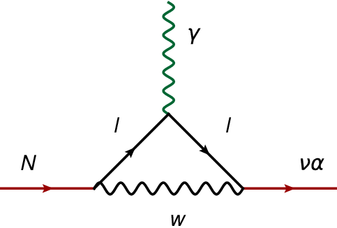
where M is the mass of the right handed neutrino and the coupling constant $\mathcal{G}$ arises from the one-loop radiative corrections, Fig(1), where after some calculation one has

$$\mathcal{G}\approx\frac{\sqrt{2}}{2\pi^{2}}\,g_{\text{\tiny{R}}}G_{\text{\tiny{F}}}\,e\,m_{l}.$$

(19)

Now by substituting (19) into (18), we arrive at the following relation

$$\Gamma(\nu_{\text{\tiny{R}}}\rightarrow\nu_{\text{\tiny{L}}}+\gamma)=\frac{\alpha}{4\pi^{4}}\,G_{\text{\tiny{F}}}^{2}\,\,m_{\ell}^{2}\,M^{3}\,g_{\text{\tiny{R}}}^{2}.$$

(20)

Therefore, by requiring that the right handed neutrino lifetime being longer than the age of the Universe $t_{\text{\tiny{Universe}}}=4.4\times 10^{17}\,\text{sec}$ [52], $g_{\text{\tiny{R}}}$ should be constrained as

$$g_{\text{\tiny{R}}}^{2}\lesssim 10^{-2}\,(\frac{1.7{\rm\ GeV}}{m_{l}})^{2}\,(\frac{1\text{eV}}{\text{M}})^{3}.$$

(21)

It should be noted that the interaction given in (12) for the right handed neutrinos is very similar to (9) for the Sterile neutrinos. Furthermore, comparing (17) with the obtained constraints on $\theta^{2}$ shows they are more or less in the same range. Therefore, there is no difference between the scattering of cosmic photons from the right handed neutrino or the Sterile one. In fact, the obtained results in the next sections can be applied for both particles on the same footing.

Several reports for the polarization measurement for the GRBs have been prepared during recent years. For instance, the linear polarization of the prompt emission from GRB 021206 has been reported at the level of $80\%$[65]. The GRB polarimeter (GAP) has observed $70\%$ and $84\%$ degrees of linear polarization of GRB 110301A and GRB 110721A, respectively [66]. Furthermore, the linear and circular polarization at afterglow radiation in GRB 121024A have been reported of the order of $28\%$ and $0.6\%$, respectively [67]. However, the linear polarization of GRB is mostly originated from synchrotron emission [68]. Meanwhile, the GRB circular polarization can be generated either due to a large-scale ordered magnetic field or Faraday conversion at the late time of the GRB radiation [15, 16, 17, 19].

In this subsection, we will consider the GRB photon-sterile neutrino forward scattering and estimate the Faraday conversion phase shift in two cases: (i) GRB photons at the prompt emission interacting with Sterile neutrinos passing through internal and external shocks, (ii) GRB photons at the afterglow intermediate emission interacting with Sterile neutrinos on the way of their propagation.

Based on the time evolution of the V-Stokes parameter in (30) and considering (69), the Faraday conversion of the scattered photons from the Sterile neutrinos evolve as follows

$$\Delta\phi_{\text{\tiny{FC}}}|_{\text{GRB}}\,=\,\frac{\sqrt{2}}{6\pi}\,\alpha\,G_{\text{\tiny{F}}}\,\theta^{2}\,\int\frac{dt}{p_{0}}\,f_{\text{\tiny{DM}}}({\bf{x}})\,v^{2}_{\text{\tiny{DM}}}\,(\hat{v}_{\alpha}\,\hat{q}_{\beta}\,\epsilon_{1}^{\alpha}\,\epsilon_{1}^{\beta}-\hat{v}_{\alpha}\,\hat{q}_{\beta}\,\epsilon_{2}^{\alpha}\,\epsilon_{2}^{\beta}),$$

(33)

where $f_{\text{\tiny{DM}}}({\bf{x}})$ is proportional to the mass density of WDM as $\rho_{\text{\tiny{DM}}}({\bf{x}})=Mf_{\text{\tiny{DM}}}({\bf{x}})$ and $p_{0}=|{\bf p}|$.

There are two possibilities for the forward scattering of GRB photons from Sterile neutrino: i) At the prompt emission level, ii) At the afterglow intermediate interaction level. The former is strongly model dependent and the polarization of high energy GRBs can be produced by scattering from WDM located close to the GRB prompt emission location. Meanwhile, the latter is model independent as the polarization of afterglow GRB photons are affected by scattering from Sterile neutrinos on their way to reach the detector.

We first estimate the Faraday conversion caused by the prompt emission-Sterile neutrino scattering. We consider a simple model in which the Sterile neutrino WDM can abundantly be produced in supernovae cores. Therefore, by scattering off the local Sterile neutrino, the linear polarization of the GRB photons at the prompt emission level can be converted to the circular polarization as

$$\Delta\phi_{\text{\tiny{FC}}}|_{\text{GRB}}\,=\,\,10^{-32}\theta^{2}\,(1+z)^{2}\,\,\,\,\,(\frac{{\rm\ GeV}}{p_{0}})(\frac{\rho_{\text{\tiny{DM}}}}{10^{-41}{\rm\ GeV}^{4}})\,(\frac{v_{\text{\tiny{DM}}}}{10^{-3}})^{2}\int\frac{dl}{10^{10}\text{cm}}\,(\hat{v}_{\alpha}\,\hat{v}_{\beta}\,\epsilon_{1}^{\alpha}\,\epsilon_{1}^{\beta}-\hat{v}_{\alpha}\,\hat{v}_{\beta}\,\epsilon_{2}^{\alpha}\,\epsilon_{2}^{\beta}),$$

(34)

where the mass density of the Sterile neutrinos is assumed to be $\rho_{\text{\tiny{DM}}}\sim 10^{-41}{\rm\ GeV}^{4}$ [70] and we have supposed that the Prompt $\gamma$-ray emission occurs at distance $\sim 10^{10}$ cm from the center.

However, in the second case, the afterglow radiation caused by the GRB photons can interact with the Sterile neutrinos in its way to the earth. Therefore, the GRB linear polarization is expected to be suppressed by the Faraday conversion phase shift. The integration over time in (33) can alternatively convert to integration over the redshift as $\int_{t^{\prime}}^{0}dt=\int_{0}^{z^{\prime}}dz/[(1+z)H(z)]$ with $H(z)=H_{0}[(\Omega_{r}(1+z)^{4}+\Omega_{M}(1+z)^{3}+\Omega_{\Lambda}]$ where $\Omega_{r}\simeq 10^{-4}$, $\Omega_{M}\simeq 0.3$ and $\Omega_{\Lambda}\simeq 0.7$ are the present densities of radiation, matter plus DM and dark energy, respectively, and $H_{0}=67.4\text{km/s/Mpc}$ is the value of Hobble constant at the present time [69]. Meanwhile, the bulk velocity of WDM, number density and energy of contributing particles depend on the redshift [71, 72] as

$$v_{\text{\tiny{DM}}}\,=\,v_{\text{\tiny{0DM}}}\,(1+z)^{-1/2},\,\,\,\,\,\,\,\,\,p_{0}=p_{0,0}(1+z),\,\,\,\,\,\,\,\,\,\ \rho_{\text{\tiny{DM}}}=\rho_{\text{\tiny{DM0}}}(1+z)^{3},$$

(35)

where $v_{\text{\tiny{0DM}}}$, $p_{0,0}$ and $n_{\text{\tiny{0DM}}}$ are obtained at the present time.

By taking (33) into account and integrating over the red shift $z$, the Faraday conversion can be estimated as follows

$$\Delta\phi_{\text{\tiny{FC}}}|_{\text{GRB}}\,=\,10^{-14}\theta^{2}\,\,(\frac{\rm\ keV}{p_{0}})\,\,\,(\frac{\rho_{\text{\tiny{DM}}}}{10^{-47}{\rm\ GeV}^{4}})\,(\frac{v_{\text{\tiny{DM}}}}{10^{-3}})^{2},$$

(36)

where we have supposed that the Sterile neutrino has the same global mass density of DM today $\rho_{\text{\tiny{DM}}}\simeq 10^{-47}{\rm\ GeV}^{4}$[69]. Conventionally, one can rewrite the above equation as a function of the decay rate and the mass of Sterile neutrino (see (10)). Therefore, the Faraday conversion due to the GRB photon-Sterile neutrino scattering depends on the mass of the Sterile neutrino as follows

$$\Delta\phi_{\text{\tiny{FC}}}|_{\text{GRB}}=10^{-14}(\frac{\rm\ keV}{M})^{5}(\frac{\rm\ keV}{p_{0}})\,(\frac{\rho_{\text{\tiny{DM}}}}{10^{-47}{\rm\ GeV}^{4}})\,(\frac{v_{\text{\tiny{DM}}}}{10^{-3}})^{2},$$

(37)

where the life time of the Sterile neutrino $\tau_{\text{\tiny{N}}}=\tau_{\text{\tiny{DM}}}\sim 10\times$ universe life time.

However, the Faraday conversion for the GRB afterglow spectrum scattering from the Sterile neutrinos can be estimated from (36) for different mixing angles in the range $\theta^{2}\approx 10^{-2}-10^{-6}$ as are shown in Tab.1.

The radio synchrotron radiation is emitted from astronomical radio sources. The astronomical radio sources are objects in our galaxy (the Milky Way) and extragalactic. Some of the famous candidates for the radio sources at the center of Milky Way, are galactic supermassive black hole Sagittarius A* [73] and Supernova remnants such as Cassiopeia A [74] and Crab Nebula [75]. The Centaurus A [76], Blazar S5 0716+71[77], Messier 87 (M87) [78] and Messier 81* (M81*)[79] radio galaxies are some of the notable sources of extra-galactic radio sources.
Due to the magnetic field properties of radio galaxies, radio emission should highly be polarized. The most likely process which gives rise to linear and circular polarization of some radio sources in galactic and extragalactic nuclei is Faraday rotation and conversion [80, 81]. In general, observation suggest the linearly polarization at the degree of $\sim 10\%$ mainly due to the synchrotron radiation from relativistic electrons. However, the circular polarization is less than $0.5\%$ [82, 83, 79, 84, 85, 86, 87, 88, 89, 90]. Also the circular polarization in the absence of a linear polarization has been detected as well [79, 84, 85].
Similar to the GRB photons, we estimate the Faraday conversion due to the radio radiation-Sterile neutrino interaction for the intergalactic sources as follows

	$\displaystyle\Delta\phi_{\text{\tiny{FC}}}|_{\text{\tiny{Sgr A*}}}\,$	$\displaystyle\approx$	$\displaystyle\,\,10^{-4}\theta^{2}\,(1+z)^{2}\,\,\,\,\,(\frac{6.5\times 10^{-7}\text{eV}}{p_{0}})(\frac{\rho_{\text{\tiny{DM}}}}{10^{-41}{\rm\ GeV}^{4}})\,(\frac{v_{\text{\tiny{DM}}}}{10^{-3}})^{2}$		(38)
			$\displaystyle\int\frac{dl}{2.4\times 10^{22}\text{cm}}\,(\hat{v}_{\alpha}\,\hat{v}_{\beta}\,\epsilon_{1}^{\alpha}\,\epsilon_{1}^{\beta}-\hat{v}_{\alpha}\,\hat{v}_{\beta}\,\epsilon_{2}^{\alpha}\,\epsilon_{2}^{\beta}),$

where $l$ demonstrates the distance of intergalactic radio sources from the Earth. Using (38) one can find the values of the Faraday conversion for some intergalactic radio sources with $z\ll 1$ as are listed in the first three rows of Tab. 2. Meanwhile, the Faraday conversion due to the forward scattering of radio radiation-Sterile neutrino for the radio galaxy M81* source can be estimated as

	$\displaystyle\Delta\phi_{\text{\tiny{FC}}}|_{\text{\tiny{M81*}}}\,\approx\Big(10^{-4}\theta^{2}\,(1+z)^{2}\,\,\,(\frac{\rho_{\text{\tiny{DM}}}}{10^{-41}{\rm\ GeV}^{4}})\int\frac{dl}{4\times 10^{22}\text{cm}}\,(\hat{v}_{\alpha}\,\hat{v}_{\beta}\,\epsilon_{1}^{\alpha}\,\epsilon_{1}^{\beta}-\hat{v}_{\alpha}\,\hat{v}_{\beta}\,\epsilon_{2}^{\alpha}\,\epsilon_{2}^{\beta})$
	$\displaystyle+5.35\times 10^{-8}\theta^{2}\,(1+z)^{2}\,\,\,(\frac{\rho_{\text{\tiny{DM}}}}{10^{-47}{\rm\ GeV}^{4}})\,\int\frac{dl}{1.096\times 10^{25}\text{cm}}\,(\hat{v}_{\alpha}\,\hat{v}_{\beta}\,\epsilon_{1}^{\alpha}\,\epsilon_{1}^{\beta}-\hat{v}_{\alpha}\,\hat{v}_{\beta}\,\epsilon_{2}^{\alpha}\,\epsilon_{2}^{\beta})\Big)$
	$\displaystyle\,\,\,\,\,\,\,\,\,\,\,\,\,\,\,\,\,\,\,\,\,\,\,\,\,\,\,\,\,\,\,\,\,\,\,\,\,\,\,\,\,\,(\frac{6.5\times 10^{-7}\text{eV}}{p_{0}})\,\,(\frac{v_{\text{\tiny{DM}}}}{10^{-3}})^{2},$

where the first term corresponds to the Faraday conversion effect inside the radio galaxy and the second one represents the Faraday conversion arising from photon traveling out of the radio galaxy toward the Earth. For simplicity, the DM mass density in other galaxies is considered at the same order of magnitude of the DM mass density in our galaxies. Nevertheless, the DM mass density is considered as the local DM mass density $\rho_{\text{\tiny{DM}}}=10^{-41}{\rm\ GeV}^{4}$ inside the galaxies and for the outside of galaxies it has been taken to be equal to the global mass density $10^{-47}{\rm\ GeV}^{4}$. As the second term in (4.2) in comparison with the first one shows, due to the value of the DM mass density, the effect of the Faraday conversion inside the radio galaxies is the dominant one. However, the Faraday conversion for different radio galaxies are given the Tab.2.. It should be noted that for the extra-galactic sources, DM mass density can be considered as a free parameter as well as the Sterile neutrino-neutrino mixing angle. Therefore, measurement on the Faraday conversion can open a new window to probe the DM mass density in radio galaxies.

In this section, we discuss about the circular polarization of the CMB photons in the conformal time $\eta$ due to photon-Sterile neutrino scattering. To this end, we focus on the left-hand side of the Boltzmann equation (30) including the information of photon propagation in the flat Friedman-Robertson-Walker(FRW) background space-time. As the circular polarization in presence of the scalar perturbation is dominant comparing to the vector and tensor perturbation, only the scalar perturbation is added to the metric and we neglect the vector and tensor perturbations. However, the DM distribution function is indicated as [98, 99, 100]:

$$f_{\text{\tiny{DM}}}(\vec{\mathbf{x}},\vec{\mathbf{q}},\eta)=f_{\text{\tiny{DM0}}}[1+\Psi(\vec{\mathbf{x}},\vec{\mathbf{q}},\eta)],$$

(40)

where $f_{\text{\tiny{DM0}}}(\vec{\mathbf{x}},\vec{\mathbf{q}},\eta)$ shows the zeroth-order distribution, $\Psi(\vec{\mathbf{x}},\vec{\mathbf{q}},\eta)$ is the perturbed part and $\vec{\mathbf{q}}=q\hat{\mathbf{n^{\prime}}}$ where $\hat{\mathbf{n^{\prime}}}$ indicates direction of the DM velocity. Neglecting the collision term on the right hand side of the Boltzmann equation, the phase space distribution of the Sterile neutrino can be obtain as follows

$$\frac{\partial f_{\text{\tiny{DM}}}}{\partial\eta}+i\frac{q}{\varepsilon_{\text{\tiny{DM}}}}(\vec{\mathbf{K}}\cdot\hat{\mathbf{n^{\prime}}})\Psi+\frac{d\ln f_{\text{\tiny{DM0}}}}{d\ln q}[\dot{\varphi}-i\frac{\varepsilon_{\text{\tiny{DM}}}}{q}(\vec{\mathbf{K}}\cdot\hat{\mathbf{n^{\prime}}})\psi]=0,$$

(41)

where $\varphi$ and $\psi$ indicate the scalar metric perturbation in the Newtonian gauge [101], $\vec{\mathbf{K}}$ is wave number of the Fourier modes of the scalar perturbations and $\varepsilon_{\text{\tiny{DM}}}=(q^{2}+a(\eta)^{2}\,M^{2})^{1/2}$ with the scale factor $a(\eta)$. Meanwhile, the angular dependence of the perturbation can be expanded in a series of Legendre polynomials $P_{l}(\mu^{\prime})$ as follows

$$\Psi(\vec{\mathbf{K}},q,\mu^{\prime},\eta)=\sum_{l=0}(-i)^{l}(2l+1)\Psi_{l}(\vec{\mathbf{K}},\eta)P_{l}(\mu^{\prime}),$$

(42)

with $\mu^{\prime}=\hat{\mathbf{K}}.\hat{\bf n^{\prime}}$. Now, we expand (30) in terms of $\Psi_{l}$ and $\mu^{\prime}$ as follows

	$\displaystyle\dot{V}$	$\displaystyle\simeq$	$\displaystyle\frac{\sqrt{2}}{3\pi\,p_{0}}\,\alpha\,\theta^{2}\,G_{\text{\tiny{F}}}\,\left[(\eta_{\text{\tiny{B}}}-i\,\eta_{\text{\tiny{A}}})\,\Delta_{P}^{+\,(S)}\,+\,(\eta_{\text{\tiny{B}}}+i\,\eta_{\text{\tiny{A}}})\,\Delta_{P}^{-\,(S)}\right]$		(43)
		$\displaystyle\times$	$\displaystyle\frac{4\pi}{3}(\frac{1}{(2\pi)^{3}})\int q^{2}\,dq\,\frac{q^{2}}{\varepsilon_{\text{\tiny{DM}}}}\,f_{\text{\tiny{DM0}}}[\Psi_{0}-2\Psi_{2}]\$
		$\displaystyle\simeq$	$\displaystyle\dot{\eta}_{\text{\tiny{DM}}}^{\text{\tiny{C-}}}\,\Delta_{P}^{+}\,+\,\dot{\eta}_{\text{\tiny{DM}}}^{\text{\tiny{C+}}}\,\Delta_{P}^{-},$		(44)

where

$\displaystyle\dot{\eta}_{\text{\tiny{DM}}}^{\text{\tiny{C}}\pm}\,$

$\displaystyle=$

$\displaystyle\,\dot{\eta}_{\text{\tiny{DM}}}^{\text{\tiny{C}}}\,(\eta_{\text{\tiny{B}}}\,\pm\,i\,\eta_{\text{\tiny{A}}}),\,\,\,\,\,\,\,$

(45)

with

$\displaystyle\eta_{\text{\tiny{A}}}\,$

$\displaystyle=$

$\displaystyle\,\left(\hat{\mathbf{K}}\cdot\mathbf{\epsilon}_{1}\right)^{2}-\left(\hat{\mathbf{K}}\cdot\mathbf{\epsilon}_{2}\right)^{2}\,,\,\,\,\,\,\,\,\,\,\,\eta_{\text{\tiny{B}}}\,=-2\hat{\mathbf{K}}\cdot\mathbf{\epsilon}_{1}\,\,\hat{\mathbf{K}}\cdot\mathbf{\epsilon}_{2},$

(46)

and

$$\dot{\eta}_{\text{\tiny{DM}}}^{\text{\tiny{C}}}\,=\,\frac{\sqrt{2}}{3\pi\,p_{0}}\,\alpha\,\theta^{2}\,G_{\text{\tiny{F}}}\,\frac{1}{(2\pi)^{3}}\left[\delta p_{\text{\tiny{DM}}}-(\bar{\rho}_{\text{\tiny{DM}}}+\bar{P}_{\text{\tiny{DM}}})\sigma_{\text{\tiny{DM}}}\right],$$

(47)

in which $\sigma_{\text{\tiny{DM}}}$ is shear stress and $\bar{\rho}_{\text{\tiny{DM}}}$ and $\bar{P}_{\text{\tiny{DM}}}$ are the unperturbed energy densities and pressure defined as [99]

$$\bar{\rho}_{\text{\tiny{DM}}}=\,a^{-4}\int\,q^{2}\,dq\,d\Omega\,\varepsilon_{\text{\tiny{DM}}}\,f_{\text{\tiny{DM0}}},\,\,\,\,\,\,\,\,\,\bar{P}_{\text{\tiny{DM}}}=\frac{1}{3}\,a^{-4}\int\,q^{2}\,dq\,d\Omega\,\frac{q^{2}}{\varepsilon_{\text{\tiny{DM}}}}\,f_{\text{\tiny{DM0}}},$$

(48)

$$(\bar{\rho}_{\text{\tiny{DM0}}}+\bar{P}_{\text{\tiny{DM0}}})\sigma_{\text{\tiny{DM}}}=\frac{8\pi}{3}\,a^{-4}\int\,q^{2}\,dq\,d\Omega\,\frac{q^{2}}{\varepsilon_{\text{\tiny{DM}}}}\,f_{\text{\tiny{DM0}}}\Psi_{2},$$

(49)

and $\delta P_{\text{\tiny{DM}}}$ as the perturbation of pressure is [99]

$\displaystyle\delta P_{\text{\tiny{DM}}}=\frac{4\pi}{3}\,a^{-4}\int\,q^{2}\,dq\,\frac{q^{2}}{\varepsilon_{\text{\tiny{DM}}}}f_{\text{\tiny{DM0}}}\Psi_{0},$

(50)

with

	$\displaystyle\dot{\Psi}_{0}$	$\displaystyle=$	$\displaystyle-\frac{q{\bf K}}{\varepsilon}\Psi_{1}-\dot{\phi}\frac{d\ln f_{\text{\tiny{DM0}}}}{d\ln q},$
	$\displaystyle\dot{\Psi}_{1}$	$\displaystyle=$	$\displaystyle\frac{q{\bf K}}{3\varepsilon_{\text{\tiny{DM}}}}(\Psi_{0}-2\Psi_{2})+\frac{\varepsilon_{\text{\tiny{DM}}}\,K}{3q}\psi\frac{d\ln f_{\text{\tiny{DM0}}}}{d\ln q},$
	$\displaystyle\dot{\Psi}_{l}$	$\displaystyle=$	$\displaystyle\frac{q{\bf K}}{(2l+1)\varepsilon_{\text{\tiny{DM}}}}(l\Psi_{l-1}-(l+1)\Psi_{l+1}),\,\,\,\,\,\,l\geq 2.$		(51)

Therefore, by inserting the initial condition, one can solve the above evolution equations numerically. Meanwhile, the time averaged value of the perturbations $\beta_{\text{\tiny{DM}}}=\frac{\delta p_{\text{\tiny{DM}}}}{\bar{\rho}_{\text{\tiny{DM}}}}-(\frac{\bar{\rho}_{\text{\tiny{DM}}}+\bar{P}_{\text{\tiny{DM}}}}{\bar{\rho}_{\text{\tiny{DM}}}})\sigma$ from the last scattering up to today can be estimated as the order of matter anisotropy $\bar{\beta}_{\text{\tiny{DM}}}\leq 10^{-4}$.

To illustrate how the $\dot{\eta}_{\text{\tiny{DM}}}^{\text{\tiny{C}}}$ depends on the red-shift, we have shown the $\dot{\eta}_{\text{\tiny{DM}}}^{\text{\tiny{C}}}$ as a function of the red-shift in Fig.(2). The $\dot{\eta}_{\text{\tiny{DM}}}^{\text{\tiny{C}}}$ are shown for three values of $\theta^{2}=10^{-3},10^{-2},10^{-1}$ and for two cases of the $\bar{\beta}_{\text{\tiny{DM}}}=10^{-4}$ and $10^{-5}$. As the figure shows the $\dot{\eta}_{\text{\tiny{DM}}}^{\text{\tiny{C}}}$ increases smoothly with red-shift up to $z=1$ then it increases rapidly at high red-shifts. In fact, the $\dot{\eta}_{\text{\tiny{DM}}}^{\text{\tiny{C}}}$ becomes larger for the larger value of the red-shift. Furthermore, in the presence of primordial scalar perturbations the CMB temperature and polarization anisotropy are given by the multi-pole moments as follows [102, 103]

$$\Delta^{S}_{I,P,V}(\eta,{\bf K},\mu)=\sum_{l=0}^{\infty}(2l+1)(-i)^{l}\Delta^{l}_{I,P,V}(\eta,{\bf K})P_{l}(\mu),$$

(52)

where $P_{l}(\mu)$ is the Legendre polynomial of rank $l$, and $\mu$ indicates scalar product of the CMB propagating direction and the wave vector ${\bf K}$. The time derivative in the left side can include the space-time structure and gravitational effects. Besides, the scattering of each plane wave can be described as the transport through a plane parallel medium [104, 105]. Therefore, the Boltzmann equation for linear and circular polarization (43) casts into

	$\displaystyle\frac{d}{d\eta}\,\Delta_{V}^{(S)}\,+\,i\,K\,\mu\,\Delta_{V}^{(S)}\,$	$\displaystyle=$	$\displaystyle\,C_{e\gamma}^{V}\,+\,\frac{1}{2}\,a(\eta)\,(\dot{\eta}_{\text{\tiny{DM}}}^{\text{\tiny{C}}-}\,\Delta_{P}^{+\,(S)}\,+\,\dot{\eta}_{\text{\tiny{DM}}}^{\text{\tiny{C}}+}\,\Delta_{P}^{-\,(S)}\,),$
	$\displaystyle\frac{d}{d\eta}\,\Delta_{P}^{\pm(S)}\,+\,i\,K\,\mu\,\Delta_{P}^{\pm(S)}\,$	$\displaystyle=$	$\displaystyle\,C_{e\gamma}^{\pm}\,\mp\,i\,a(\eta)\dot{\eta}^{\text{\tiny{P}}}\,\Delta_{P}^{\pm}.$		(53)

However, the value of linear polarization $\Delta p^{\pm(S)}$ and $\Delta V^{(S)}$ in the direction ${\bf\hat{n}}$ and at the present time $\eta_{0}$ can be obtained by integrating the Boltzmann equation along the line of sight [102] and over all the Fourier modes ${\bf K}$ as

	$\displaystyle\Delta_{P}^{\pm(S)}(\hat{\bf{n}})$	$\displaystyle=$	$\displaystyle\int d^{3}{\bf{K}}\xi({\bf{K}})e^{\pm 2i\phi_{K,n}}\Delta_{P}^{\pm(S)}({\mathbf{K}},{\mathbf{p}},\eta),\,\,\,\,\,$
	$\displaystyle\Delta_{V}^{(S)}(\hat{\bf{n}})$	$\displaystyle=$	$\displaystyle\int d^{3}{\bf{K}}\xi({\bf{K}})\Delta_{V}^{(S)}(\mathbf{K},\mathbf{p},\eta),\,\,\,\,\,$		(54)

where $\xi(\bf{K})$ is a random variable using to characterize the initial amplitude of the mode, $\phi_{K,n}$ is the angle required to rotate the $\bf{K}$ and $\hat{\bf{n}}$ dependent basis to a fixed frame in the sky.

Therefore we obtain

$$\Delta_{P}^{\pm(S)}(\mathbf{K},\mu,\eta_{0})=\int_{0}^{\eta_{0}}d\eta\,\dot{\eta}_{e\gamma}\,e^{ix\mu-\eta_{e\gamma}\mp i\,\eta^{\text{\tiny{P}}}_{\text{\tiny{DM}}}}\,\,\Big[{3\over 4}(1-\mu^{2})\Pi(\mathbf{K},\eta)\Big],$$

(55)

and

	$\displaystyle\Delta_{V}^{(S)}({\bf{K}},\mu,\eta_{0})\,$	$\displaystyle=$	$\displaystyle\,\frac{1}{2}\,\int_{0}^{\eta_{0}}\,d\eta\,\dot{\eta}_{e\gamma}\,e^{i\,x\,\mu\,-\eta_{e\gamma}}\,[3\mu\,\Delta_{V}^{(S)}\,+\,(\frac{\dot{\eta}_{\text{\tiny{DM}}}^{\text{\tiny{C}}-}}{\dot{\eta}_{e\gamma}}\,\Delta_{P}^{+(S)}\,+\,\frac{\dot{\eta}_{\text{\tiny{DM}}}^{\text{\tiny{C}}+}}{\dot{\eta}_{e\gamma}}\,\Delta_{P}^{-(S)})],$		(56)
		$\displaystyle\simeq$	$\displaystyle\,\frac{1}{2}\,\int_{0}^{\eta_{0}}\,d\eta\,\dot{\eta}_{e\gamma}\,e^{i\,x\,\mu\,-\eta_{e\gamma}}\,[3\mu\,\Delta_{V}^{(S)}\,+\,2\,\eta_{\text{\tiny{B}}}\,\frac{\dot{\eta}_{\text{\tiny{DM}}}^{\text{\tiny{C}}}}{\dot{\eta}_{e\gamma}}\,\Delta_{P}^{(S)}],$

where $x\,=\,{\bf{K}}\,(\eta_{0}-\eta)$, $\dot{\eta}_{e\gamma}\,=\,n_{e}\,\sigma_{T}\,\chi_{e}$ and $\eta_{e\gamma}\,=\,\int_{\eta}^{\eta_{0}}\,\dot{\eta}_{e\gamma}\,d\eta$ are the differential optical depth and total optical depth due to the Thomson scattering at time $\eta$ with $\chi_{e}$ being the ionization fraction, respectively. Moreover $\Delta p$ is defined as

$$\Delta^{(S)}_{P}({\bf{K}},\mu,\eta)=\dfrac{3}{4}(1-\mu^{2})\int_{0}^{\eta}d\eta\,e^{ix\mu-\eta_{e\gamma}}\,\dot{\eta_{e\gamma}}\,\Pi({\bf{K}},\eta),$$

(57)

with

$$\Pi\equiv\Delta^{S_{2}}_{I}+\Delta^{S_{2}}_{P}-\Delta^{S_{\circ}}_{P}.$$

(58)

References

- [1] P. Ullio and M. Kamionkowski, JHEP 0103, 049 (2001) doi:10.1088/1126-6708/2001/03/049 [hep-ph/0006183].
- [2] L. Page et al. [WMAP Collaboration], Astrophys. J. Suppl. 170, 335 (2007) doi:10.1086/513699 [astro-ph/0603450].
- [3] P. A. R. Ade et al. [Planck Collaboration], Astron. Astrophys. 571, A31 (2014) doi:10.1051/0004-6361/201423743 [arXiv:1508.03375 [astro-ph.CO]].
- [4] J. Angle et al. [XENON10 Collaboration], Phys. Rev. Lett. 107, 051301 (2011) Erratum: [Phys. Rev. Lett. 110, 249901 (2013)] doi:10.1103/PhysRevLett.110.249901, 10.1103/PhysRevLett.107.051301 [arXiv:1104.3088 [astro-ph.CO]].
- [5] E. Aprile et al. [XENON100 Collaboration], Phys. Rev. Lett. 107, 131302 (2011) doi:10.1103/PhysRevLett.107.131302 [arXiv:1104.2549 [astro-ph.CO]].
- [6] K. Abe et al. [XMASS Collaboration], Astropart. Phys. 31, 290 (2009) doi:10.1016/j.astropartphys.2009.02.006 [arXiv:0809.4413 [physics.ins-det]].
- [7] C. E. Aalseth et al. [CoGeNT Collaboration], Phys. Rev. Lett. 106, 131301 (2011) doi:10.1103/PhysRevLett.106.131301 [arXiv:1002.4703 [astro-ph.CO]].
- [8] R. Bernabei et al. [DAMA Collaboration], Eur. Phys. J. C 56, 333 (2008) doi:10.1140/epjc/s10052-008-0662-y [arXiv:0804.2741 [astro-ph]].
- [9] P. Belli, R. Bernabei, A. Bottino, F. Cappella, R. Cerulli, N. Fornengo and S. Scopel, Phys. Rev. D 84, 055014 (2011) doi:10.1103/PhysRevD.84.055014 [arXiv:1106.4667 [hep-ph]].
- [10] S. Archambault et al., Phys. Lett. B 682, 185 (2009) doi:10.1016/j.physletb.2009.11.019 [arXiv:0907.0307 [hep-ex]].
- [11] S. Archambault et al. [PICASSO Collaboration], New J. Phys. 13, 043006 (2011) doi:10.1088/1367-2630/13/4/043006 [arXiv:1011.4553 [physics.ins-det]].
- [12] P. Pani and G. Polesello, Phys. Dark Univ. 21, 8 (2018) doi:10.1016/j.dark.2018.04.006 [arXiv:1712.03874 [hep-ph]]; U. Haisch and G. Polesello, JHEP 1902, 029 (2019) doi:10.1007/JHEP02(2019)029 [arXiv:1812.00694 [hep-ph]]; A. Krovi, I. Low and Y. Zhang, JHEP 1810, 026 (2018) doi:10.1007/JHEP10(2018)026 [arXiv:1807.07972 [hep-ph]].
- [13] N. F. Bell, Y. Cai, J. B. Dent, R. K. Leane and T. J. Weiler, Phys. Rev. D 96, no. 2, 023011 (2017) doi:10.1103/PhysRevD.96.023011 [arXiv:1705.01105 [hep-ph]]; B. Penning, J. Phys. G 45, no. 6, 063001 (2018) doi:10.1088/1361-6471/aabea7 [arXiv:1712.01391 [hep-ex]]; Y. Tsai, L. T. Wang and Y. Zhao, Phys. Rev. D 93, no. 3, 035024 (2016) doi:10.1103/PhysRevD.93.035024 [arXiv:1511.07433 [hep-ph]].
- [14] R. Mohammadi, Eur. Phys. J. C 74, no. 10, 3102 (2014) doi:10.1140/epjc/s10052-014-3102-1, 10.1140/epjc/s10052-014-3089-7 [arXiv:1312.2199 [astro-ph.CO]].
- [15] E. Bavarsad, M. Haghighat, Z. Rezaei, R. Mohammadi, I. Motie and M. Zarei, Phys. Rev. D 81, 084035 (2010) doi:10.1103/PhysRevD.81.084035 [arXiv:0912.2993 [hep-th]].
- [16] A. Cooray, A. Melchiorri and J. Silk, Phys. Lett. B 554, 1 (2003) doi:10.1016/S0370-2693(02)03291-4 [astro-ph/0205214].
- [17] S. Tizchang, S. Batebi, M. Haghighat and R. Mohammadi, Eur. Phys. J. C 76, no. 9, 478 (2016) doi:10.1140/epjc/s10052-016-4312-5 [arXiv:1605.09045 [hep-ph]].
- [18] N. Bartolo, A. Hoseinpour, S. Matarrese, G. Orlando and M. Zarei, arXiv:1903.04578 [hep-ph].
- [19] S. Batebi, R. Mohammadi, R. Ruffini, S. Tizchang and S. S. Xue, Phys. Rev. D 94, no. 6, 065033 (2016) doi:10.1103/PhysRevD.94.065033 [arXiv:1610.01154 [astro-ph.HE]].
- [20] S. Alexander and E. McDonough, Phys. Lett. B 789, 197 (2019) doi:10.1016/j.physletb.2018.12.037 [arXiv:1811.05953 [astro-ph.CO]].
- [21] P. Kumar and B. Zhang, Phys. Rept. 561, 1 (2014) doi:10.1016/j.physrep.2014.09.008 [arXiv:1410.0679 [astro-ph.HE]].
- [22] S. E. Woosley, Astrophys. J. 405, 273 (1993). doi:10.1086/172359; K. Iwamoto et al., Nature 395, 672 (1998) doi:10.1038/27155 [astro-ph/9806382]. ; G. Preparata, R. Ruffini, S.-S. Xue, “The dyadosphere of black holes and gamma-ray bursts’, Astronomy and Astrophysics, v.338, p.L87-L90 (1998); “On the Dyadosphere of Black Hole ” J.Korean Phys.Soc.42:S99-S104,2003, arXiv:astro-ph/0204080 ; A. MacFadyen and S. E. Woosley, Astrophys. J. 524, 262 (1999) doi:10.1086/307790 [astro-ph/9810274].
- [23] N. Gehrels and S. Razzaque, Front. Phys. (Beijing) 8, 661 (2013) doi:10.1007/s11467-013-0282-3 [arXiv:1301.0840 [astro-ph.HE]].
- [24] T. Piran, Rev. Mod. Phys. 76, 1143 (2004) doi:10.1103/RevModPhys.76.1143 [astro-ph/0405503].
- [25] Chambers, K.C., Miley, G.K., Joyce, R.R. (1988), Astrophysical Journal, L75-L79.
- [26] Tabatabaei, F. S., Schinnerer, E., Krause, M., et al. 2017, ApJ, 836, 185
- [27] Tadhunter, C. N., Scarrott, S. M., Draper, P., Rolph, C. 1992, MNRAS, 256, 53P.
- [28] Tadhunter, C. N., Scarrott, S. M., Draper, P., Rolph, C. 1992, MNRAS, 256, 53P.
- [29] Cimatti, A., di Serego Alighieri, S., Fosbury, R. A. E., Salvati, M., Taylor, D. 1993, MNRAS, 264, 421.
- [30] C. S. Frenk and S. D. M. White, Annalen Phys. 524, 507 (2012) doi:10.1002/andp.201200212 [arXiv:1210.0544 [astro-ph.CO]].
- [31] T. Lin, arXiv:1904.07915 [hep-ph]; J. Redondo, PoS NOW 2018, 083 (2019). doi:10.22323/1.337.0083; M. Bastero-Gil, J. Santiago, L. Ubaldi and R. Vega-Morales, JCAP 1904, no. 04, 015 (2019) doi:10.1088/1475-7516/2019/04/015 [arXiv:1810.07208 [hep-ph]].
- [32] A. Boyarsky, M. Drewes, T. Lasserre, S. Mertens and O. Ruchayskiy, Prog. Part. Nucl. Phys. 104, 1 (2019) doi:10.1016/j.ppnp.2018.07.004 [arXiv:1807.07938 [hep-ph]].
- [33] K. N. Abazajian et al., arXiv:1204.5379 [hep-ph].
- [34] S. S. Xue, JHEP 1611, 072 (2016) doi:10.1007/JHEP11(2016)072 [arXiv:1605.01266 [hep-ph]]
- [35] S. S. Xue, Mod. Phys. Lett. A 14, 2701 (1999) doi:10.1142/S0217732399002844 [hep-ph/9706301].
- [36] T. Asaka and M. Shaposhnikov, Phys. Lett. B 620, 17 (2005) doi:10.1016/j.physletb.2005.06.020 [hep-ph/0505013].
- [37] M. Shaposhnikov, JHEP 0808, 008 (2008) doi:10.1088/1126-6708/2008/08/008 [arXiv:0804.4542 [hep-ph]].
- [38] A. Boyarsky, O. Ruchayskiy and M. Shaposhnikov, Ann. Rev. Nucl. Part. Sci. 59, 191 (2009) doi:10.1146/annurev.nucl.010909.083654 [arXiv:0901.0011 [hep-ph]].
- [39] T. Asaka, S. Blanchet and M. Shaposhnikov, Phys. Lett. B 631, 151 (2005) doi:10.1016/j.physletb.2005.09.070 [hep-ph/0503065].
- [40] S. Dodelson and L. M. Widrow, Phys. Rev. Lett. 72, 17 (1994) doi:10.1103/PhysRevLett.72.17 [hep-ph/9303287].
- [41] P. Minkowski, Phys. Lett. 67B, 421 (1977). doi:10.1016/0370-2693(77)90435-X; S. L. Glashow, NATO Sci. Ser. B 61, 687 (1980). doi:10.1007/978-1-4684-7197-7-15; M. Gell-Mann, P. Ramond and R. Slansky, Conf. Proc. C 790927, 315 (1979) [arXiv:1306.4669 [hep-th]]; T. Yanagida, Prog. Theor. Phys. 64, 1103 (1980). doi:10.1143/PTP.64.1103; J. Schechter and J. W. F. Valle, Phys. Rev. D 22, 2227 (1980). doi:10.1103/PhysRevD.22.2227
- [42] R. N. Mohapatra and G. Senjanovic, Phys. Rev. Lett. 44, 912 (1980). doi:10.1103/PhysRevLett.44.912
- [43] T. P. Cheng and L. F. Li, Phys. Rev. D 22, 2860 (1980). doi:10.1103/PhysRevD.22.2860 ; R. N. Mohapatra and G. Senjanovic, Phys. Rev. D 23, 165 (1981). doi:10.1103/PhysRevD.23.165
- [44] R. Foot, H. Lew, X. G. He and G. C. Joshi, Z. Phys. C 44, 441 (1989). doi:10.1007/BF01415558
- [45] A. Kusenko, F. Takahashi and T. T. Yanagida, Phys. Lett. B 693, 144 (2010) doi:10.1016/j.physletb.2010.08.031 [arXiv:1006.1731 [hep-ph]].
- [46] P. Cox, C. Han and T. T. Yanagida, JCAP 1801, no. 01, 029 (2018) doi:10.1088/1475-7516/2018/01/029 [arXiv:1710.01585 [hep-ph]].
- [47] L. Canetti, M. Drewes, T. Frossard and M. Shaposhnikov, Phys. Rev. D 87, 093006 (2013) doi:10.1103/PhysRevD.87.093006 [arXiv:1208.4607 [hep-ph]] ; A. Merle, Int. J. Mod. Phys. D 22, 1330020 (2013) doi:10.1142/S0218271813300206 [arXiv:1302.2625 [hep-ph]]; D. Gorbunov, A. Khmelnitsky and V. Rubakov, JCAP 0810, 041 (2008) doi:10.1088/1475-7516/2008/10/041 [arXiv:0808.3910 [hep-ph]]; S. Horiuchi, P. J. Humphrey, J. Onorbe, K. N. Abazajian, M. Kaplinghat and S. Garrison-Kimmel, Phys. Rev. D 89, no. 2, 025017 (2014) doi:10.1103/PhysRevD.89.025017 [arXiv:1311.0282 [astro-ph.CO]] ; K. C. Y. Ng, S. Horiuchi, J. M. Gaskins, M. Smith and R. Preece, Phys. Rev. D 92, no. 4, 043503 (2015) doi:10.1103/PhysRevD.92.043503 [arXiv:1504.04027 [astro-ph.CO]]; A. Schneider, PoS NOW 2016, 093 (2017) doi:10.22323/1.283.0093 [arXiv:1704.01832 [astro-ph.CO]] ; N. Menci, A. Grazian, A. Lamastra, F. Calura, M. Castellano and P. Santini, Astrophys. J. 854, no. 1, 1 (2018) doi:10.3847/1538-4357/aaa773 [arXiv:1801.03697 [astro-ph.CO]]; R. Yunis, C. R. Argüelles, N. E. Mavromatos, A. Moliné, A. Krut, J. A. Rueda and R. Ruffini, arXiv:1810.05756 [astro-ph.GA]; K. C. Y. Ng, B. M. Roach, K. Perez, J. F. Beacom, S. Horiuchi, R. Krivonos and D. R. Wik, Phys. Rev. D 99, 083005 (2019) doi:10.1103/PhysRevD.99.083005 [arXiv:1901.01262 [astro-ph.HE]]; L. Johns and G. M. Fuller, arXiv:1903.08296 [hep-ph]; K. Kadota and K. Kaneta, Phys. Rev. D 97, no. 11, 115021 (2018) doi:10.1103/PhysRevD.97.115021 [arXiv:1702.04526 [hep-ph]].
- [48] F. Bezrukov, A. Chudaykin and D. Gorbunov, JCAP 1706, no. 06, 051 (2017) doi:10.1088/1475-7516/2017/06/051 [arXiv:1705.02184 [hep-ph]].
- [49] M. Drewes, Int. J. Mod. Phys. E 22, 1330019 (2013) doi:10.1142/S0218301313300191 [arXiv:1303.6912 [hep-ph]].
- [50] P. B. Pal and L. Wolfenstein, Phys. Rev. D 25, 766 (1982). doi:10.1103/PhysRevD.25.766
- [51] V. D. Barger, R. J. N. Phillips and S. Sarkar, Phys. Lett. B 352, 365 (1995) Erratum: [Phys. Lett. B 356, 617 (1995)] doi:10.1016/0370-2693(95)00486-5, 10.1016/0370-2693(95)00831-5 [hep-ph/9503295].
- [52] P. A. R. Ade et al. [Planck Collaboration], Astron. Astrophys. 594, A13 (2016) doi:10.1051/0004-6361/201525830 [arXiv:1502.01589 [astro-ph.CO]].
- [53] A. D. Dolgov, Phys. Rept. 370, 333 (2002) doi:10.1016/S0370-1573(02)00139-4 [hep-ph/0202122].
- [54] E. Holzschuh, W. Kundig, L. Palermo, H. Stussi and P. Wenk, Phys. Lett. B 451, 247 (1999). doi:10.1016/S0370-2693(99)00200-2
- [55] J. N. Abdurashitov et al., Pisma Zh. Eksp. Teor. Fiz. 105, no. 12, 723 (2017) [JETP Lett. 105, no. 12, 753 (2017)] doi:10.1134/S0021364017120013 [arXiv:1703.10779 [hep-ex]].
- [56] S. S. Xue, Phys. Rev. D 93, no. 7, 073001 (2016) doi:10.1103/PhysRevD.93.073001 [arXiv:1506.05994 [hep-ph]].
- [57] S. S. Xue, Phys. Lett. B 398, 177 (1997) doi:10.1016/S0370-2693(97)00213-X [hep-ph/9610508].
- [58] S. Alioli, V. Cirigliano, W. Dekens, J. de Vriesdan, E. Mereghetti JHEP05(2017)086; ArXiv ePrint:1703.04751
- [59] M. Tanabashi et al. [Particle Data Group], Phys. Rev. D 98 (2018) no.3, 030001. doi:10.1103/PhysRevD.98.030001
- [60] A. Kosowsky, Annals Phys. 246, 49 (1996) doi:10.1006/aphy.1996.0020 [astro-ph/9501045].
- [61] A. G. Pacholczyk, MNRAS 163, P29 (1973).
- [62] M. Kennett and D. Melrose, PASA, 15, 211 (1998).
- [63] M. Zaldarriaga, D. N. Spergel and U. Seljak, Astrophys. J. 488, 1 (1997) doi:10.1086/304692 [astro-ph/9702157].
- [64] W. Hu and M. J. White, New Astron. 2, 323 (1997) doi:10.1016/S1384-1076(97)00022-5 [astro-ph/9706147].
- [65] W. Coburn and S. E. Boggs, Nature 423, 415 (2003) doi:10.1038/nature01612 [astro-ph/0305377].
- [66] D. Yonetoku et al., Astrophys. J. Lett. 758, no. 1, L1 (2012) doi:10.1088/2041-8205/758/1/L1 [arXiv:1208.5287 [astro-ph.HE]].
- [67] K. Wiersema et al., Nature 509, 201 (2014) doi:10.1038/nature13237 [arXiv:1410.0489 [astro-ph.HE]].
- [68] Troja, E., Lipunov, V. M., Mundell, C. G., et al. 2017, Nature, 547, 425
- [69] N. Aghanim et al. [Planck Collaboration], arXiv:1807.06209 [astro-ph.CO].
- [70] T. Güver, A. E. Erkoca, M. Hall Reno and I. Sarcevic, JCAP 1405, 013 (2014) doi:10.1088/1475-7516/2014/05/013 [arXiv:1201.2400 [hep-ph]].
- [71] W. Hu, Astrophys. J. 529, 12 (2000) doi:10.1086/308279 [astro-ph/9907103].
- [72] A. Vahedi, J. Khodagholizadeh, R. Mohammadi and M. Sadegh, JCAP 1901, no. 01, 052 (2019) doi:10.1088/1475-7516/2019/01/052 [arXiv:1809.08137 [astro-ph.CO]].
- [73] D. J. Munoz, D. P. Marrone, J. M. Moran and R. Rao, Astrophys. J. 745, 115 (2012) doi:10.1088/0004-637X/745/2/115 [arXiv:1105.0427 [astro-ph.HE]].
- [74] R. A. Fesen et al., Astrophys. J. 645, 283 (2006) doi:10.1086/504254 [astro-ph/0603371].
- [75] A. Ritacco et al., Astron. Astrophys. 616, A35 (2018) doi:10.1051/0004-6361/201731551 [arXiv:1804.09581 [astro-ph.CO]].
- [76] M. Zemcov et al. [QUaD Collaboration], Astrophys. J. 710, 1541 (2010) doi:10.1088/0004-637X/710/2/1541 [arXiv:0908.2431 [astro-ph.CO]].
- [77] E. Cenacchi, A. Kraus, T. Beckert and K.-H. Mack, ASP Conf. Ser. 449, 426 (2011) [arXiv:0901.4678 [astro-ph.IM]].
- [78] C. Y. Kuo et al., Astrophys. J. 783, L33 (2014) doi:10.1088/2041-8205/783/2/L33 [arXiv:1402.5238 [astro-ph.GA]].
- [79] A. Brunthaler, G. C. Bower and H. Falcke, Astron. Astrophys. [J. Phys. Conf. Ser. 54, 474 (2006)] doi:10.1088/1742-6596/54/1/074 [astro-ph/0601474].
- [80] M. Tucci and L. Toffolatti, Adv. Astron. 2012, 624987 (2012) doi:10.1155/2012/624987 [arXiv:1204.0427 [astro-ph.CO]].
- [81] A. Gruzinov and Y. Levin, Astrophys. J. 876 (2019) no.1, 74 doi:10.3847/1538-4357/ab0fa3 [arXiv:1902.01485 [astro-ph.HE]].
- [82] T. Beckert and H. Falcke, Astron. Astrophys. 388, 1106 (2002) doi:10.1051/0004-6361:20020484 [astro-ph/0112398].
- [83] D. P. Rayner, R. P. Norris and R. J. Sault, Mon. Not. R. Astron. Soc. 319, 484 (2000)
- [84] A. Brunthaler, G. C. Bower, H. Falcke and R. R. Mellon, Astrophys. J. 560, L123 (2001) doi:10.1086/324308 [astro-ph/0109170].
- [85] D. Mesa, C. Baccigalupi, G. De Zotti, L. Gregorini, K. H. Mack, M. Vigotti and U. Klein, Astron. Astrophys. 396, 463 (2002) doi:10.1051/0004-6361:20021392 [astro-ph/0209502].
- [86] G. C. Bower, H. Falcke and D. C. Backer, Astrophys. J. 523, L29 (1999) doi:10.1086/312246 [astro-ph/9907215].
- [87] G. C. Bower, H. Falcke, R. J. Sault and D. C. Backer, Astrophys. J. 571, 843 (2002) doi:10.1086/340064 [astro-ph/0202138].
- [88] H. Wiesemeyer , C. Thum ,D. Morris ,J. Aumont ,C. Rosset , ,AA, 528, A11 (2011)
- [89] A. S. Wilson and K. W. Weiler, ApJ, 475, 661 (1997)
- [90] M. C. H. Wright and J. R. Forster, ApJ, 239, 873 (1980)
- [91] A. Jiménez-Rosales and J. Dexter, Mon. Not. Roy. Astron. Soc. 478, no. 2, 1875 (2018) doi:10.1093/mnras/sty1210 [arXiv:1805.02652 [astro-ph.HE]].
- [92] W. Raja and A. A. Deshpande, ASI Conference Series, 13, 275 (2014)
- [93] D. L. Kaplan, S. Chatterjee, B. M. Gaensler and J. Anderson, Astrophys. J. 677, 1201 (2008) doi:10.1086/529026 [arXiv:0801.1142 [astro-ph]].
- [94] E. Ros and M. A. Perez-Torres, Astron. Astrophys. 537, A93 (2012) doi:10.1051/0004-6361/201118399 [arXiv:1111.4856 [astro-ph.CO]].
- [95] S. Bird, W. E. Harris, J. P. Blakeslee and C. Flynn, Astron. Astrophys. 524, A71 (2010) doi:10.1051/0004-6361/201014876 [arXiv:1009.3202 [astro-ph.GA]].
- [96] D. J. Majaess, Acta Astron. 60, 121 (2010) [arXiv:1006.2458 [astro-ph.CO]].
- [97] V. M. Larionov et al., Astrophys. J. 768, 40 (2013) doi:10.1088/0004-637X/768/1/40 [arXiv:1303.2218 [astro-ph.HE]].
- [98] Scott Dodelson, Modern Cosmology, ACADEMIC PRESS, (2003).
- [99] C. P. Ma and E. Bertschinger, Astrophys. J. 455, 7 (1995) doi:10.1086/176550 [astro-ph/9506072].
- [100] J. Lesgourgues and S. Pastor, Phys. Rept. 429, 307 (2006) doi:10.1016/j.physrep.2006.04.001 [astro-ph/0603494].
- [101] V.F. Mukhanov, H.A. Feldman, and R.H. Brandenberger, Phys. Rep.215, 203 (1992).
- [102] M. Zaldarriaga and U. Seljak, Phys. Rev. D 55, 1830 (1997) doi:10.1103/PhysRevD.55.1830 [astro-ph/9609170].
- [103] U. Seljak and M. Zaldarriaga, Astrophys. J. 469, 437 (1996) doi:10.1086/177793 [astro-ph/9603033].
- [104] S. Chandrasekhar, “Radiative Transfer”, Dover, New York, 1960.
- [105] N. Kaiser, Mon. Not. R. Astron. Soc. 202, 1169 (1983).
- [106] Gorbunov, D.S. and Rubakov, ”V.A.- Introduction to the Theory of the Early Universe Cosmological Perturbations and Inflationary Theory” - World Scientific Publishing Company Incorporated (2011)
- [107] F. Della Valle, A. Ejlli, U. Gastaldi, G. Messineo, E. Milotti, R. Pengo, G. Ruoso and G. Zavattini, Eur. Phys. J. C 76, no. 1, 24 (2016) doi:10.1140/epjc/s10052-015-3869-8 [arXiv:1510.08052 [physics.optics]].
- [108] I. L. Padilla et al., arXiv:1911.00391 [astro-ph.CO].
- [109] Sazonov V. N., 1969, Sov. Astron., 13, 396.
- [110] Sazonov V. N., Tsytovich V. N., 1968, Radiophys. Quant. Electron., 11, 731.
- [111] Pacholczyk A. G., 1970, Radio astrophysics. Nonthermal processes in galactic and extragalactic sources. W.H.Freeman and Co Ltd, SanFrancisco, pp. 77–111.
- [112] J. Y. Chan, K. Wu, A. Y. On, D. J. Barnes, J. D. McEwen and T. D. Kitching, Mon. Not. Roy. Astron. Soc. 484, no.2, 1427-1455 (2019) doi:10.1093/mnras/sty3498 [arXiv:1901.04581 [astro-ph.CO]].
- [113] L. Huang and R. V. Shcherbakov, Mon. Not. Roy. Astron. Soc. 416, 2574 (2011) doi:10.1111/j.1365-2966.2011.19207.x [arXiv:1106.1630 [astro-ph.HE]].