跳到论文正文
W Papers独立论文阅读器 arXiv:1909.03735 论文正文 计算阅读时间 · 0%
引用这篇论文根据当前论文元数据生成,正式投稿前建议核对。


License: arXiv.org perpetual non-exclusive license
arXiv:1909.03735v1 [math.CA] 09 Sep 2019

A constructive approach towards the Method of Solution-Regions

F. Adrián F. Tojo Note: The author was partially supported by Ministerio de Economía y Competitividad, Spain, and FEDER, project MTM2013-43014-P, and by the Agencia Estatal de Investigación (AEI) of Spain under grant MTM2016-75140-P, co-financed by the European Community fund FEDER. Affiliation: e-mail: fernandoadrian.fernandez@usc.es Affiliation: Instituto de Matemáticas, Facultade de Matemáticas, Affiliation: Universidade de Santiago de Compostela, Spain.
Abstract

In this work we develop the theory of solution-regions with a constructive approach. We also extend the theory to the case of general linear conditions and provide various sets of sufficient hypotheses for existence and multiplicity results.

Keywords: System of First Order Differential Equations, Multiple Solutions, Fixed Point Index, General Boundary Conditions, Solution-Regions, Upper and Lower Solutions

MSC: Primary 34B15; secondary 34A34, 34A12

1 Introduction

In a recent paper of Frigon [6] the author developed a theory, named method of solution-regions, in order to obtain results concerning the existence and multiplicity of solutions of the equation

u′​(t)=f⁡(t,u⁡(t))​ for a.e. ​t∈I:=[a,b],u∈B,u^{\prime}(t)=f(t,u(t))\text{ for a.e. }t\in I:=[a,b],\ u\in B, (1.1)

where II is a non-degenerate interval and BB is the family of functions satisfying initial conditions of the form

u⁡(a)=ru(a)=r (1.2)

or the periodic boundary conditions

u⁡(a)=u⁡(b).u(a)=u(b). (1.3)

The method of solution-regions is an outstanding generalization of various methods of obtaining uniqueness and multiplicity of solutions of differential problems, namely the methods of upper and lower solutions [18, 8], strict upper and lower solutions [20, 12, 4], solution-tubes [5, 9] and strict solution-tubes [5, 7]. Furthermore, the method is closely related to that of Gaines and Mahwin concerning what they called bound sets [11, 10]. The definition of bound set extends that of solution region in the way presented in Remark 3.5, but the theory concerning them is developed in a non-comparable way as we will point out.

In this paper we take a constructive approach towards admissible regions. It is in Section 2 that we prove that, indeed, admissible regions, such as are defined in Definition 2.3, always have an admissible pair, something which formed part of the assumptions before [6, Definition 3.1]. By unlinking the topological and analytical aspects of admissible regions we are able to reach many interesting conclusions regarding their nature (see Remarks 2.5 and 3.3).

In what concerns solution regions (Section 3) we state the refined definition of CC-solution region. This parameter dependent definition relaxes the restrictions imposed on the admissible pair (condition (H5)) while maintaining a simple proof. We also provide some alternative or complementary hypotheses (see (H4’), (H5’) and (H6)) in order to derive, in the next section, existence results.

In Section 4 we generalize the problems studied in [6] by allowing more general boundary conditions. First we deal with general linear conditions of the kind

�⁡(u−u⁡(a))=r,\Gamma(u-u(a))=r, (1.4)

where r∈Rr\in{\mdmathbb R} and �:𝒞⁡([a,b],R)→R\Gamma:{\mathcal{C}}([a,b],{\mdmathbb R})\to{\mdmathbb R} is a linear functional (which can be thought as �:𝒞⁡([a,b],Rn)→Rn\Gamma:{\mathcal{C}}([a,b],{\mdmathbb R}^{n})\to{\mdmathbb R}^{n} by action on each component) such that M:=�⁡(1)≠0M:=\Gamma(1)\neq 0 (11 understood as the constant function 11 on [a,b][a,b]). Observe that, by Riesz–Markov–Kakutani Representation Theorem [1, Theorem 7.2.4], there is a unique regular Borel (signed) measure �\mu on [a,b][a,b] such that �​u=∫u​d⁡�\Gamma u=\int u\operatorname{d}\mu for every u∈𝒞⁡([a,b],R)u\in{\mathcal{C}}([a,b],{\mdmathbb R}). Also, condition (1.4) generalizes condition (1.3). Just take r=0r=0 and �​u=u⁡(b)\Gamma u=u(b) (observe that �⁡(1)=1≠0\Gamma(1)=1\neq 0).

We will also work with the boundary condition

�​u=r,\Gamma u=r, (1.5)

It is clear that that condition (1.5) generalizes condition (1.2) by defining �\Gamma as before. Also, observe that conditions (1.4) and (1.5) overlap in some cases, but neither of them covers all of the cases of the other. At the end of Section 4 we provide an example to which the theory is applied.

In Section 5 we deal with multiplicity results in the usual way through Fixed Point Index Theory. This scenario requires refined hypotheses (such as (H0’), (H4”) and (H5”)).

Finally we present our conclusions in Section 6, where we talk about the prowess and limitations of this approach and present some guidelines to overcome the occurring difficulties.

Throughout this paper we will work with the spaces Rn{\mdmathbb R}^{n} with the euclidean norm ∥⋅∥\|\cdot\| and 𝒞⁡(X,Rn){\mathcal{C}}(X,{\mdmathbb R}^{n}) the space of continuous functions with the supremum norm ∥⋅∥0\|\cdot\|_{0} where XX is some set. R+{\mdmathbb R}^{+} will denote the interval (0,+∞)(0,+\infty).

2 Admissible Regions

Let us first state some basic definitions for the theory ahead.

Definition 2.1.

Let A⊂R×RnA\subset{\mdmathbb R}\times{\mdmathbb R}^{n}. Given t∈Rt\in{\mdmathbb R} and x∈Rnx\in{\mdmathbb R}^{n} we write

At:={x∈Rn:(t,x)∈A},A_{t}:=\{x\in{\mdmathbb R}^{n}\ :\ (t,x)\in A\},

and

Ax:={t∈R:(t,x)∈A}.A^{x}:=\{t\in{\mdmathbb R}\ :\ (t,x)\in A\}.

If we consider the continuous natural inclusions it:Rn→R×Rni_{t}:{\mdmathbb R}^{n}\to{\mdmathbb R}\times{\mdmathbb R}^{n} and ix:R→R×Rni^{x}:{\mdmathbb R}\to{\mdmathbb R}\times{\mdmathbb R}^{n} such that it​(x)=ix​(t)=(t,x)i_{t}(x)=i^{x}(t)=(t,x), then At=(it)−1​(A)A_{t}=(i_{t})^{-1}(A) and Ax=(ix)−1​(A)A^{x}=(i^{x})^{-1}(A). Similarly, we consider the natural projections �1:R×Rn→R\pi_{1}:{\mdmathbb R}\times{\mdmathbb R}^{n}\to{\mdmathbb R} and �2:R×Rn→Rn\pi_{2}:{\mdmathbb R}\times{\mdmathbb R}^{n}\to{\mdmathbb R}^{n} such that �1​(t,x)=t\pi_{1}(t,x)=t and �2​(t,x)=x\pi_{2}(t,x)=x.

Definition 2.2 ([6, Definition 2.1]).

Let D⊂I×RnD\subset I\times{\mdmathbb R}^{n}. A map f:D→Rmf:D\to{\mdmathbb R}^{m} is a Carathéodory function if

  1. 1.

    f⁡(t,⋅)f(t,\cdot) is continuous on DtD_{t} for almost every t∈It\in I,

  2. 2.

    f⁡(⋅,x)f(\cdot,x) is measurable for all x∈�2​(R)x\in\pi_{2}(R),

  3. 3.

    for all k∈R+k\in{\mdmathbb R}^{+}, there exists ∈kL1(I,R){}_{k}\in L^{1}(I,{\mdmathbb R}) such that ∥f(t,x)∥≤(t)k\|f(t,x)\|\leq{}_{k}(t) for a. e. tt and every xx such that ‖x‖≤k\|x\|\leq k and (t,x)∈D(t,x)\in D, that is, the set

    {t∈I:∥f(t,x)∥>(t)k for some x∈Rt,∥x∥≤k}\{t\in I\ :\ \|f(t,x)\|>{}_{k}(t)\text{ for some }x\in R_{t},\ \|x\|\leq k\}

    has measure zero.

Definition 2.3.

Let n∈Nn\in{\mdmathbb N}. A set R⊂I×RnR\subset I\times{\mdmathbb R}^{n}, is called an admissible region if RR is compact and

  1. (H0)

    Rt≠∅R_{t}\neq\emptyset for every t∈It\in I.

Definition 2.4.

Let R⊂I×RnR\subset I\times{\mdmathbb R}^{n} be an admissible region. A pair of continuous functions (h,p)(h,p) where h:I×Rn→Rh:I\times{\mdmathbb R}^{n}\to{\mdmathbb R} and p=(p1,p2):I×Rn→I×Rnp=(p_{1},p_{2}):I\times{\mdmathbb R}^{n}\to I\times{\mdmathbb R}^{n} is called an admissible pair associated to RR if

  • (H1)

    R=h−1((−∞,0])R=h^{-1}{((-\infty,0])}.

  • (H2)

    The map hh has partial derivatives at (t,x)(t,x) for almost every tt and every xx with (t,x)∈(I×Rn)\R(t,x)\in(I\times{\mdmathbb R}^{n})\backslash R and ∂h∂t\frac{\partial h}{\partial t} and ∇xh\nabla_{x}h are locally Carathéodory maps on (I×Rn)\R(I\times{\mdmathbb R}^{n})\backslash R.

  • (H3)

    pp is bounded and such that p⁡(t,x)=(t,x)p(t,x)=(t,x) for every (t,x)∈R(t,x)\in R and

    ⟨∇xh​(t,x),p2​(t,x)−x⟩≤0​ for a. e. t and every x with (t,x)∈(I×Rn)\R.\left\langle\nabla_{x}h(t,x),p_{2}(t,x)-x\right\rangle\leq 0\text{ for a.\,e. $t$ and every $x$ with $(t,x)\in(I\times{\mdmathbb R}^{n})\backslash R$.} (2.1)
Remark 2.5.

There are several things to take into account in this definition.

  1. 1.

    The definition of admissible region in [6] is more stringent in condition (2.1), where the inequality is taken in the strict sense. We will show that this is not necessary in order to get the same results, provided that we add another condition, (H6), later on, or that we alter condition (H4) ahead (see Remark 4.6).

  2. 2.

    The definition of admissible region in [6] imposes the existence of an associated admissible pair (that is, it includes axioms (H1)-(H3) in the definition), something which we prove is always the case.

  3. 3.

    The definition of admissible region in [6] does not require explicitly RR to be compact, although that is a direct consequence of it.

  4. 4.

    How do we interpret the set on which condition (2.1) holds? In the proof of [6, Theorem 5.1] they use that, for any function u∈W1,1​(I,Rn)u\in W^{1,1}(I,{\mdmathbb R}^{n}) such that (t,u⁡(t))∈R(t,u(t))\in R and for every t∈It\in I almost everywhere on {t:h⁡(t,u⁡(t))>0}\{t\ :\ h(t,u(t))>0\},

    ⟨∇xh​(t,u⁡(t)),p2​(t,u⁡(t))−u⁡(t)⟩<0.\left\langle\nabla_{x}h(t,u(t)),p_{2}(t,u(t))-u(t)\right\rangle<0.

    In order to ensure this inequality holds in terms of a variable xx instead of u⁡(t)u(t) it is enough to have that the set

    {t∈I:⟨∇xh​(t,x),p2​(t,x)−x⟩≥0​ for some ​x∈Rt}\{t\in I\ :\ \left\langle\nabla_{x}h(t,x),p_{2}(t,x)-x\right\rangle\geq 0\text{ for some }x\in R_{t}\}

    has measure zero.

  5. 5.

    In [6] the author highlighted, by providing several examples, the versatility of admissible regions, showing that they may have corners, their boundary may not be smooth and that they may not be proximate retracts. With the definition presented here it is obvious that those are possibilities for admissible regions.

  6. 6.

    If (h,p)(h,p) is an admissible pair and �∈𝒞1​(I,R+)\beta\in{\mathcal{C}}^{1}(I,{\mdmathbb R}^{+}), then (h~,p)(\widetilde{h},p) is also an admissible pair where h~​(t,x)=�​(t)​h​(t,x)\widetilde{h}(t,x)=\beta(t)h(t,x). Hence, if h⁡(t,Rt)h(t,R_{t}) is bounded for every t∈It\in I, taking �\beta such that �​(t)<1/sup‖h⁡(t,Rt)‖\beta(t)<1/\sup\|h(t,R_{t})\|, we have that h~\widetilde{h}, defined as before, is bounded.

  7. 7.

    If (hk,p)(h_{k},p) are an admissible pairs for k=1,2k=1,2; then (h1+h2,p)(h_{1}+h_{2},p) is an admissible pair.

Now we are ready to state some definitions and results in order to construct an admissible pair for a given region function.

Definition 2.6.

Let C,D⊂RnC,D\subset{\mdmathbb R}^{n}. We define the distance of a point xx to the set CC as

dC​(x):=inf{‖x−y‖:y∈C}.d_{C}(x):=\inf\{||x-y||\ :\ y\in C\}.

Analogously, we define the distance between CC and DD as

d(C,D):=inf{||x−y||:x∈C,y∈D}.d(C,D):=\inf\{||x-y||\ :\ x\in C,\ y\in D\}.

Furthermore, if CC is convex, we denote by PC:Rn→CP_{C}:{\mdmathbb R}^{n}\to C the projection onto CC. Remember that PCP_{C} is a continuous function [14, p. 108].

Theorem 2.7 ([14, p. 63]).

Let CC be a closed convex subset of a Hilbert space HH, and let '​(x):=12​dC​(x)2\varphi(x):=\frac{1}{2}d_{C}(x)^{2} for every x∈Hx\in H. Then '\varphi is a C1C^{1} convex function on HH and ∇'​(x)=x−PC​(x)\nabla\varphi(x)=x-P_{C}(x).

Proposition 2.8 ([16, Proposition 3.3.6]).

Let R⊂RnR\subset{\mdmathbb R}^{n} be a closed set. Then there is
'∈𝒞∞(Rn,[0,+∞))\varphi\in{\mathcal{C}}^{\infty}({\mdmathbb R}^{n},[0,+\infty)) such that '−1​(0)=R\varphi^{-1}(0)=R.

Remark 2.9.

Observe that, in Proposition 2.8, since '\varphi attains an absolute minimum at every point of RR, ∇'​(x)=0\nabla\varphi(x)=0 for every x∈Rx\in R.

Theorem 2.10.

Let R⊂I×RnR\subset I\times{\mdmathbb R}^{n} be an admissible region. Then RR has an associated admissible pair (h,p)(h,p).

Proof.

Let r∈R+r\in{\mdmathbb R}^{+} such that �2​(R)⊂C:=BRn​[0,r]\pi_{2}(R)\subset C:=B_{{\mdmathbb R}^{n}}[0,r]. Let D:=BRn​(0,r+1)D:=B_{{\mdmathbb R}^{n}}(0,r+1) and ':Rn+1→R\varphi:{\mdmathbb R}^{n+1}\to{\mdmathbb R} be the function provided by Proposition 2.8 for R∪(I×(Rn\D))R\cup(I\times({\mdmathbb R}^{n}\backslash D)). Define

h⁡(t,x):={'​(t,x),(t,x)∈I×C,[1−dC​(x)2]​'​(t,x)+12​dC​(x)2,(t,x)∈I×(D\C),12​dC​(x)2,(t,x)∈I×(Rn\D).h(t,x):=\begin{cases}\varphi(t,x),&(t,x)\in I\times C,\\ [1-d_{C}(x)^{2}]\varphi(t,x)+\frac{1}{2}d_{C}(x)^{2},&(t,x)\in I\times(D\backslash C),\\ \frac{1}{2}d_{C}(x)^{2},&(t,x)\in I\times({\mdmathbb R}^{n}\backslash D).\end{cases}

hh is of class 𝒞1{\mathcal{C}}^{1} and R=h−1((−∞,0])R=h^{-1}((-\infty,0]), so (H1) and (H2) are satisfied. In fact,

∇xh​(t,x):={∇x'​(t,x),(t,x)∈I×C,−2​[x−PC​(x)]​'​(t,x)+[1−dC​(x)2]​∇x'​(t,x)+x−PC​(x),(t,x)∈I×(D\C),x−PC​(x),(t,x)∈I×(Rn\D).\nabla_{x}h(t,x):=\begin{cases}\nabla_{x}\varphi(t,x),&(t,x)\in I\times C,\\ -2[x-P_{C}(x)]\varphi(t,x)+[1-d_{C}(x)^{2}]\nabla_{x}\varphi(t,x)+x-P_{C}(x),&(t,x)\in I\times(D\backslash C),\\ x-P_{C}(x),&(t,x)\in I\times({\mdmathbb R}^{n}\backslash D).\end{cases}

Furthermore, ∇xh​(t,x)=0\nabla_{x}h(t,x)=0 for every (t,x)∈R(t,x)\in R (see Remark 2.9). Let p=(p1,p2):I×Rn→I×Rnp=(p_{1},p_{2}):I\times{\mdmathbb R}^{n}\to I\times{\mdmathbb R}^{n} with p1​(t,x)=tp_{1}(t,x)=t and p2​(t,x):=x−∇xh​(t,x)=p_{2}(t,x):=x-\nabla_{x}h(t,x)=

{x−∇x'​(t,x),(t,x)∈I×C,2​[x−PC​(x)]​'​(t,x)−[1−dC​(x)2]​∇x'​(t,x)+PC​(x),(t,x)∈I×(D\C),PC​(x),(t,x)∈I×(Rn\D).\begin{cases}x-\nabla_{x}\varphi(t,x),&(t,x)\in I\times C,\\ 2[x-P_{C}(x)]\varphi(t,x)-[1-d_{C}(x)^{2}]\nabla_{x}\varphi(t,x)+P_{C}(x),&(t,x)\in I\times(D\backslash C),\\ P_{C}(x),&(t,x)\in I\times({\mdmathbb R}^{n}\backslash D).\end{cases}

pp is continuous, bounded, and p⁡(t,x)=(t,x)p(t,x)=(t,x) for every (t,x)∈R(t,x)\in R. Furthermore,

⟨∇xh​(t,x),p2​(t,x)−x⟩=−‖∇xh​(t,x)‖2≤0,\left\langle\nabla_{x}h(t,x),p_{2}(t,x)-x\right\rangle=-\|\nabla_{x}h(t,x)\|^{2}\leq 0,

so (H3) holds as well.

∎

3 Solution Regions

In the previous section we have presented the basic aspects of admissible regions, including the construction of admissible pairs. Unfortunately, the properties of these regions are independent of the problem of study (in this case problem (1.1)). It is for this reason that we need the concept of solutions regions.

Definition 3.1.

Let C∈R+C\in{\mdmathbb R}^{+}. A triple (R,(h,p))(R,(h,p)) where R⊂I×RnR\subset I\times{\mdmathbb R}^{n} is an admissible region and (h,p)(h,p) is an admissible pair for RR is called a CC-solution region of problem (1.1), if the following hold:

  1. (H4)

    ∂h∂t​(t,x)+⟨∇xh​(t,x),f⁡(p⁡(t,x))⟩≤0\frac{\partial h}{\partial t}(t,x)+\left\langle\nabla_{x}h(t,x),f(p(t,x))\right\rangle\leq 0 for a.e. tt and every xx with (t,x)∉R(t,x)\not\in R.

  2. (H5)

    h⁡(a,u⁡(a))≤0h(a,u(a))\leq 0 or h⁡(a,u⁡(a))≤h⁡(b,u⁡(b))h(a,u(a))\leq h(b,u(b)) for any u∈Bu\in B such that ‖u‖0≤C\|u\|_{0}\leq C.

Remark 3.2.

In [6] they talk about solution regions and not CC-solution regions. We will use this extra information given by the parameter CC for the more general boundary conditions (1.4) and (1.5) we deal with in this work.

Remark 3.3.

We can rewrite condition (H4) as ⟨∇h​(t,x),f~​(p⁡(t,x))⟩≤0\left\langle\nabla h(t,x),\widetilde{f}(p(t,x))\right\rangle\leq 0 for a.e. tt and every xx with (t,x)∉R(t,x)\not\in R where f~=(1,f)\widetilde{f}=(1,f). Written in this way, this expression is reminiscent of the transversality condition [3, Equation (2.1)], necessary for some generalized Lipschitz uniqueness results, where f~\widetilde{f} is the function defined to transform a non-autonomous problem into an autonomous one.

Thus expressed, (H4) has a geometric interpretation similar to the transversality condition. The function ∇h​(t,x)\nabla h(t,x) can be thought as a normal field to the local foliation in I×RnI\times{\mdmathbb R}^{n} where the leaves are defined by h−1​(c)h^{-1}(c) for each value c∈Rc\in{\mdmathbb R}. Hence, (H4) implies that the function f~\widetilde{f} points, at each point in h−1​(c)h^{-1}(c), in the direction of decreasing value of cc, that is, against the flow ∇h​(t,x)\nabla h(t,x) that takes one leave to another.

Remark 3.4.

In this article we will only use the statement of (H5) in the case conditions BB refer to conditions (1.4) or (1.5). The reader can check that, for the cases (1.2) and (1.3) (studied in [6]), condition (H5) can be rewritten as

  • •

    h⁡(a,r)≤0h(a,r)\leq 0 or h⁡(a,u⁡(a))≤h⁡(b,x)h(a,u(a))\leq h(b,x) for any x∈Rnx\in{\mdmathbb R}^{n}, ‖x‖≤C\|x\|\leq C in the case of condition (1.2) and

  • •

    h⁡(a,x)≤0h(a,x)\leq 0 or h⁡(a,x)≤h⁡(b,x)h(a,x)\leq h(b,x) for any x∈Rnx\in{\mdmathbb R}^{n}, ‖x‖≤C\|x\|\leq C.

They are used with a similar statement in [6].

Remark 3.5.

The concept of solution region is closely related to that of bound set in [11, 10].

Definition 3.6 ([10]).

We say that a set A⊂I×RnA\subset I\times{\mdmathbb R}^{n} is a bound set relative to problem (1.1) if

  1. 1.

    AA is open in the relative topology of I×RnI\times{\mdmathbb R}^{n}.

  2. 2.

    For any (t0,x0)∈∂A(t_{0},x_{0})\in\partial A with t0∈(a,b)t_{0}\in(a,b) there exists V∈𝒞1​(I×Rn,R)V\in{\mathcal{C}}^{1}(I\times{\mdmathbb R}^{n},{\mdmathbb R}) such that

    1. (a)

      A⊂V−1​(−∞,0)A\subset V^{-1}(-\infty,0),

    2. (b)

      V⁡(t0,x0)=0V(t_{0},x_{0})=0,

    3. (c)

      ∂V∂t​(t0,x0)+⟨∇xV​(t0,x0),f⁡(t0,x0)⟩≠0\frac{\partial V}{\partial t}(t_{0},x_{0})+\left\langle\nabla_{x}V(t_{0},x_{0}),f(t_{0},x_{0})\right\rangle\neq 0.

Let (R,(h,p))(R,(h,p)) be a solution region of problem (1.1). and consider A:=R̊A:=\mathring{R}. AA is open in the relative topology of I×RnI\times{\mdmathbb R}^{n}. Fix (t0,x0)∈∂A(t_{0},x_{0})\in\partial A. Using Proposition 2.8, let ∈𝒞∞​(I×Rn,Rn)\psi\in{\mathcal{C}}^{\infty}(I\times{\mdmathbb R}^{n},{\mdmathbb R}^{n}) such that ≥0\psi\geq 0 and (0)−1=Rn\A{}^{-1}(0)={\mdmathbb R}^{n}\backslash A. Let V=h− V=h-\psi. Taking the functional VV for every (t0,x0)∈∂A(t_{0},x_{0})\in\partial A we can show that AA is a bound set relative to problem (1.1). Clearly, in the relative topology of I×RnI\times{\mdmathbb R}^{n}, not all compact sets are the closure of an open set and not all open sets have compact closures but, in practice, bound sets generalize solution regions.

The results concerning bound sets in [10] have a different flavor than those presented here. For instance they require bound sets to be autonomous, that is, with VV independent of t0t_{0} and tt –cf. [10, Definition 3.2] and the ff occurring in problem (1.1) has to be continuous –see [10, Theorem 3.1].

As said before, in [6], the inequality in condition (2.1) is taken in the strict sense. We will need the following condition to make up for it.

  • (H6)

    Let (R,(h,p))(R,(h,p)) be a solution region of problem (1.1). Then there exists h^\widehat{h} such that (R,(h^,p))(R,(\widehat{h},p)) is a solution region of problem (1.1) and there exist t1,t2∈It_{1},t_{2}\in I such that h^​(t1,x)=h⁡(t1,x)\widehat{h}(t_{1},x)=h(t_{1},x) for every x∈Rnx\in{\mdmathbb R}^{n} and h^​(t2,x)≠h⁡(t2,x)\widehat{h}(t_{2},x)\neq h(t_{2},x) for every x∈Rn\Rt2x\in\ {\mdmathbb R}^{n}\backslash R_{t_{2}}.

In the light of Remark 2.5, points 6 and 7, condition (H6) is not as stringent as it may seem. In this line, the following lemma shows a sufficient condition for (H6) to hold.

Lemma 3.7.

Let (R,(h,p))(R,(h,p)) be a solution region for (1.1). Assume that hh is bounded and (h,p)(h,p) satisfies

  1. (H4’)

    There exist "∈R+\varepsilon\in{\mdmathbb R}^{+}, �∈R+\delta\in{\mdmathbb R}^{+} and t0∈I̊t_{0}\in\mathring{I} such that t∈[t0−�,t0+�]⊂I̊t\in[t_{0}-\delta,t_{0}+\delta]\subset\mathring{I} and

    ∂h∂t​(t,x)+⟨∇xh​(t,x),f⁡(p⁡(t,x))⟩≤−",\frac{\partial h}{\partial t}(t,x)+\left\langle\nabla_{x}h(t,x),f(p(t,x))\right\rangle\leq-\varepsilon,

    for a.e. t∈[t0−�,t0+�]t\in[t_{0}-\delta,t_{0}+\delta] and every xx with (t,x)∉R(t,x)\not\in R.

Then (H6) holds.

Proof.

Let �∈𝒞1​(I,R+)\beta\in{\mathcal{C}}^{1}(I,{\mdmathbb R}^{+}) such that �|I\[t0−�,t0+�]=1\beta|_{I\backslash[t_{0}-\delta,t_{0}+\delta]}=1 and �​(t)>1\beta(t)>1 for t∈(t0−�,t0+�)t\in(t_{0}-\delta,t_{0}+\delta), ‖�′‖0<"/‖h‖0\|\beta^{\prime}\|_{0}<\varepsilon/\|h\|_{0} for t∈It\in I. Define h^​(t,x)=�​(t)​h​(t,x)\widehat{h}(t,x)=\beta(t)h(t,x) for every (t,x)∈I×Rn(t,x)\in I\times{\mdmathbb R}^{n}. Clearly, (h^,p)(\widehat{h},p) is an admissible pair and h^​(a,x)=h​(a,x)\widehat{h}(a,x)=h(a,x) and h^​(b,x)=h​(b,x)\widehat{h}(b,x)=h(b,x), so h^\widehat{h} satisfies (H5). Also h^​(t0,x)≠h⁡(t0,x)\widehat{h}(t_{0},x)\neq h(t_{0},x) for every x∈Rt0x\in R_{t_{0}}.

Furthermore,

∂h^∂t​(t,x)+⟨∇xh^​(t,x),f⁡(p⁡(t,x))⟩\displaystyle\frac{\partial\widehat{h}}{\partial t}(t,x)+\left\langle\nabla_{x}\widehat{h}(t,x),f(p(t,x))\right\rangle
=\displaystyle= �′​(t)​h​(t,x)+�​(t)​∂h∂t​(t,x)+⟨∇x(�​h)​(t,x),f⁡(p⁡(t,x))⟩\displaystyle\beta^{\prime}(t)h(t,x)+\beta(t)\frac{\partial h}{\partial t}(t,x)+\left\langle\nabla_{x}(\beta h)(t,x),f(p(t,x))\right\rangle
=\displaystyle= �′​(t)​h​(t,x)+�​(t)​[∂h∂t​(t,x)+⟨∇xh​(t,x),f⁡(p⁡(t,x))⟩]\displaystyle\beta^{\prime}(t)h(t,x)+\beta(t)\left[\frac{\partial h}{\partial t}(t,x)+\left\langle\nabla_{x}h(t,x),f(p(t,x))\right\rangle\right]
≤\displaystyle\leq �′​(t)​h​(t,x)−�​(t)​"≤‖�′‖0​‖h‖0−"≤0.\displaystyle\beta^{\prime}(t)h(t,x)-\beta(t)\varepsilon\leq\|\beta^{\prime}\|_{0}\|h\|_{0}-\varepsilon\leq 0.

∎

4 Existence results

Now we recall the following lemma which will be the key to proving various results ahead. We present it in a slightly modified way, although the proof is the same as in [6].

Lemma 4.1 ([6, Lemma 2.3]).

Let z∈Rz\in{\mdmathbb R}, w∈𝒞⁡(I,R)w\in{\mathcal{C}}(I,{\mdmathbb R}) and J=w−1​((,,,))J=w^{-1}((z,+\infty)). Assume that

  1. 1.

    w∈Wloc1,1​(J,R)w\in W^{1,1}_{\operatorname{loc}}(J,{\mdmathbb R}),

  2. 2.

    w′​(t)≤0w^{\prime}(t)\leq 0 for a. e. t∈Jt\in J,

  3. 3.

    one of the following conditions holds:

    1. (a)

      w⁡(a)≤zw(a)\leq z,

    2. (b)

      w⁡(a)≤w⁡(b)w(a)\leq w(b).

Then w⁡(t)≤zw(t)\leq z for all t∈It\in I or there exists k>0k>0 such that w⁡(t)=kw(t)=k for all t∈It\in I.

Remark 4.2.

In Lemma 4.1, if w′​(t)<0w^{\prime}(t)<0 for a. e. t∈Jt\in J, then ww cannot be constant so, in that case, w⁡(t)≤zw(t)\leq z.

Let (h,p)(h,p) be an admissible pair associated to an admissible region RR. Consider again r∈Rnr\in{\mdmathbb R}^{n} and a positive linear functional �:𝒞⁡(I,R)→R\Gamma:{\mathcal{C}}(I,{\mdmathbb R})\to{\mdmathbb R}. Let M:=�⁡(1)M:=\Gamma(1). In what follows we will assume M>0M>0. In the case we would like to work with a functional �\Gamma such that M<0M<0, it is enough to do the change of variables v=−uv=-u and study the problem v′​(t)=f~​(t,v⁡(t))v^{\prime}(t)=\widetilde{f}(t,v(t)), �~​(v−v​(a))=r\widetilde{\Gamma}(v-v(a))=r ( �~​v=r\widetilde{\Gamma}v=r respectively), where f~​(t,x)=−f⁡(t,−x)\widetilde{f}(t,x)=-f(t,-x) and �~=−�\widetilde{\Gamma}=-\Gamma.

Define g⁡(s):=�⁡(�[a,⋅]​(s))g(s):=\Gamma(\chi_{[a,\cdot]}(s)) for every s∈Is\in I where �[a,t]​(s)\chi_{[a,t]}(s) denotes the characteristic function of of the interval [a,t][a,t]. Observe that gg is nonnegative. Let c∈L1​(I,R)c\in L^{1}(I,{\mdmathbb R}) be such that c⁡(t)>‖f⁡(p⁡(t,x))‖c(t)>\|f(p(t,x))\| for a. e. t∈It\in I and every x∈Rnx\in{\mdmathbb R}^{n}. Now, define

fR​(t,x):={f⁡(t,x),(t,x)∈R,f⁡(p⁡(t,x))+c⁡(t)​(p2​(t,x)−x),(t,x)∈(I×Rn)\R,f_{R}(t,x):=\begin{cases}f(t,x),&(t,x)\in R,\\ f(p(t,x))+c(t)(p_{2}(t,x)-x),&(t,x)\in(I\times{\mdmathbb R}^{n})\backslash R,\end{cases}

and

�​u:=�​∫atfR​(s,u⁡(s))​d⁡s.\Theta u:=\Gamma\int_{a}^{t}f_{R}(s,u(s))\operatorname{d}s.

Since �​u=∫u​d⁡�\Gamma u=\int u\operatorname{d}\mu for some unique regular Borel measure �\mu on II, we can apply Fubini’s Theorem [1, Theorem 3.7.5], and so

�​u=�​∫abfR​(s,u⁡(s))​�[a,t]​(s)​d​s=∫abfR​(s,u⁡(s))​g​(s)​d​s.\Theta u=\Gamma\int_{a}^{b}f_{R}(s,u(s))\chi_{[a,t]}(s)\operatorname{d}s=\int_{a}^{b}f_{R}(s,u(s))g(s)\operatorname{d}s.

Let m:=max⁡{‖x‖:x∈�2​(R)}m:=\max\{\|x\|\ :\ x\in\pi_{2}(R)\}, C:=max⁡{m,1+‖p2‖0}C:=\max\left\{m,1+\|p_{2}\|_{0}\right\}, K>CK>C, D:=BRn​[0,C]D:=B_{{\mdmathbb R}^{n}}[0,C], E:=BRn​(0,K)E:=B_{{\mdmathbb R}^{n}}(0,K) and 𝒰:={u∈𝒞⁡(I,Rn):‖u‖0<K}{\mathcal{U}}:=\{u\in{\mathcal{C}}(I,{\mdmathbb R}^{n})\ :\ \|u\|_{0}<K\}.

With the previous ingredients we can consider the problem

u′​(t)=\displaystyle u^{\prime}(t)= �​fR​(t,u⁡(t)),\displaystyle\lambda f_{R}(t,u(t)), (4.1)
u⁡(a)=\displaystyle u(a)= PD​(�​u−rM).\displaystyle P_{D}\left(\frac{\Gamma u-r}{M}\right). (4.2)

Observe that condition (4.2) is equivalent to �⁡(u−u⁡(a))=r\Gamma(u-u(a))=r when u∈Du\in D. The reason for the projection is that, due to the nature of the boundary condition (1.4), we cannot, in general, bound ‖u⁡(a)‖\|u(a)\| (unlike in the cases of (1.2) and (1.3), cf. [6]) which is necessary in order for condition 3.(a) in Lemma 4.1 to be satisfied. A similar approach using a projection in the case of upper and lower solutions was used in [2, Section 3], where the nonlinear condition L1​(u⁡(a),u⁡(b),u′​(a),u′​(b),u)=0L_{1}(u(a),u(b),u^{\prime}(a),u^{\prime}(b),u)=0 occurred.

We could have presented ondition (4.2) as

M​u​(a)=PM​D​(�​u−r),Mu(a)=P_{MD}\left(\Gamma u-r\right), (4.3)

where M​D:={M​x∈Rn:x∈D}MD:=\{Mx\in{\mdmathbb R}^{n}\ :\ x\in D\} thanks to the following lemma. Observe that, although (4.3) would allow to write condition (4.2) for the case M=0M=0, doing this would be fruitless: for M=0M=0 condition (4.3) reads 0=00=0.

Lemma 4.3.

For any �∈[0,+∞)\alpha\in[0,+\infty), x∈Rnx\in{\mdmathbb R}^{n}, we have that �​PD​(x)=P�​D​(�​x)\alpha P_{D}(x)=P_{\alpha D}\left(\alpha x\right).

Proof.

We have that

�​PD​(x)={�​x,‖x‖≤C,�​C​x‖x‖,‖�​x‖>C,P�​D​(�​x)={�​x,‖�​x‖≤�​C,�​C​�​x‖�​x‖,‖�​x‖>�​C.\alpha P_{D}(x)=\begin{cases}\alpha x,&\|x\|\leq C,\\ \alpha C\frac{x}{\|x\|},&\|\alpha x\|>C,\end{cases}\quad P_{\alpha D}\left(\alpha x\right)=\begin{cases}\alpha x,&\|\alpha x\|\leq\alpha C,\\ \alpha C\frac{\alpha x}{\|\alpha x\|},&\|\alpha x\|>\alpha C.\end{cases}

Written this way, the result is clear. ∎

Let, �​u:=�​u−PM​D​(�​u−r)\displaystyle\Phi u:=\Gamma u-P_{MD}\left(\Gamma u-r\right) and consider the operator 𝒥:[0,1]×𝒞⁡(I,Rn)→𝒞⁡(I,Rn){\mathcal{J}}:[0,1]\times{\mathcal{C}}(I,{\mdmathbb R}^{n})\to{\mathcal{C}}(I,{\mdmathbb R}^{n}) defined by

𝒥⁡(�,u):=u⁡(a)+�​∫atfR​(s,u⁡(s))​d⁡s−(1+�​(t−a))​(�​�​u−�​u).{\mathcal{J}}(\lambda,u):=u(a)+\lambda\int_{a}^{t}f_{R}(s,u(s))\operatorname{d}s-(1+\lambda(t-a))(\lambda\Theta u-\Phi u).

Inspired in [6], we present the following results concerning the existence of solutions.

Proposition 4.4.

Let f:I×Rn→Rnf:I\times{\mdmathbb R}^{n}\to{\mdmathbb R}^{n} be a Carathéodory function and (h,p)(h,p) an admissible pair associated to an admissible region RR. Assume (H6) holds and M>0M>0. Then, for every �∈[0,1]\lambda\in[0,1], problem (4.1),(4.2) has at least one solution. Moreover, ind⁡(𝒥⁡(�,⋅),𝒰)=(−1)n\operatorname{ind}({\mathcal{J}}(\lambda,\cdot),{\mathcal{U}})=(-1)^{n} for every �∈[0,1]\lambda\in[0,1].

Proof.

𝒥{\mathcal{J}} is a continuous and completely continuous operator (cf. [6, Lemma 2.2]). Also, the fixed points of ℐ{\mathcal{I}} are solutions of (4.1),(4.2). Indeed, if u=𝒥⁡(�,u)u={\mathcal{J}}(\lambda,u) then, for every t∈It\in I,

u⁡(t)=u⁡(a)+�​∫atfR​(s,u⁡(s))​d⁡s−(1+�​(t−a))​(�​�​u−�​u).u(t)=u(a)+\lambda\int_{a}^{t}f_{R}(s,u(s))\operatorname{d}s-(1+\lambda(t-a))(\lambda\Theta u-\Phi u).

In particular, for t=at=a, we get that �​�​u=�​u\lambda\Theta u=\Phi u, so

u⁡(t)=u⁡(a)+�​∫atfR​(s,u⁡(s))​d⁡s.u(t)=u(a)+\lambda\int_{a}^{t}f_{R}(s,u(s))\operatorname{d}s. (4.4)

Applying �\Gamma to both sides in (4.4), we obtain �​u=M​u​(a)+�​�​u=M​u​(a)+�​u\Gamma u=Mu(a)+\lambda\Theta u=Mu(a)+\Phi u. Hence,

u⁡(a)=�​u−�​uM=PD​(�​u−rM),u(a)=\frac{\Gamma u-\Phi u}{M}=P_{D}\left(\frac{\Gamma u-r}{M}\right),

and condition (4.2) is satisfied. Also, for a. e. t∈It\in I,

u′​(t)=�​fR​(t,u⁡(t)),u^{\prime}(t)=\lambda f_{R}(t,u(t)),

so uu is a solution of (4.1),(4.2) for every �∈[0,1]\lambda\in[0,1].

Now we prove that the solutions of (4.1),(4.2) are bounded by CC. Assume uu is a solution of equation (4.1),(4.2) for some �∈[0,1]\lambda\in[0,1], that is,

u⁡(t)=u⁡(a)+�​∫atfR​(s,u⁡(s))​d⁡s.u(t)=u(a)+\lambda\int_{a}^{t}f_{R}(s,u(s))\operatorname{d}s.

Consider first the case �=0\lambda=0. In that case u≡xu\equiv x for some constant x∈Rnx\in{\mdmathbb R}^{n}, so

‖u‖0=‖x‖=‖u⁡(a)‖=‖PD​(�​u−rM)‖≤C.\|u\|_{0}=\|x\|=\|u(a)\|=\left\|P_{D}\left(\frac{\Gamma u-r}{M}\right)\right\|\leq C.

Now we study the case �>0\lambda>0.

Then, almost everywhere on {t∈I:‖u⁡(t)‖>C}\{t\in I\ :\ \|u(t)\|>C\},

‖u⁡(t)‖′=\displaystyle\|u(t)\|^{\prime}= ⟨u⁡(t)‖u⁡(t)‖,u′​(t)⟩=⟨u⁡(t)‖u⁡(t)‖,�​fR​(s,u⁡(t))⟩\displaystyle\left\langle\frac{u(t)}{\|u(t)\|},u^{\prime}(t)\right\rangle=\left\langle\frac{u(t)}{\|u(t)\|},\lambda f_{R}(s,u(t))\right\rangle
=\displaystyle= ⟨u⁡(t)‖u⁡(t)‖,�​[f⁡(p⁡(t,u⁡(t)))+c⁡(t)​(p2​(t,u⁡(t))−u⁡(t))]⟩\displaystyle\left\langle\frac{u(t)}{\|u(t)\|},\lambda[f(p(t,u(t)))+c(t)(p_{2}(t,u(t))-u(t))]\right\rangle
=\displaystyle= −�​c​(t)|u⁡(t)|+⟨u⁡(t)‖u⁡(t)‖,�​[f⁡(p⁡(t,u⁡(t)))+c⁡(t)​p2​(t,u⁡(t))]⟩\displaystyle-\lambda c(t)\|u(t)\|+\left\langle\frac{u(t)}{\|u(t)\|},\lambda[f(p(t,u(t)))+c(t)p_{2}(t,u(t))]\right\rangle
≤\displaystyle\leq −�​c​(t)​C+|⟨u⁡(t)‖u⁡(t)‖,�​[f⁡(p⁡(t,u⁡(t)))+c⁡(t)​p2​(t,u⁡(t))]⟩|\displaystyle-\lambda c(t)C+\left|\left\langle\frac{u(t)}{\|u(t)\|},\lambda[f(p(t,u(t)))+c(t)p_{2}(t,u(t))]\right\rangle\right|
≤\displaystyle\leq �​c​(t)​(1+‖p2‖0−C)<0,\displaystyle\lambda c(t)\left(1+\|p_{2}\|_{0}-C\right)<0,

where the last inequality is a consequence of the definition of cc. Then, by Lemma 4.1 and Remark 4.2, ‖u‖0≤C\|u\|_{0}\leq C.

By the homotopy property of the fixed point index, ind⁡(𝒥⁡(�,⋅),𝒰)=ind⁡(𝒥⁡(0,⋅),𝒰)\operatorname{ind}({\mathcal{J}}(\lambda,\cdot),{\mathcal{U}})=\operatorname{ind}({\mathcal{J}}(0,\cdot),{\mathcal{U}}) for every �∈[0,1]\lambda\in[0,1].

Observe that

𝒥⁡(0,u)​(t)=u⁡(a)+�​u.{\mathcal{J}}(0,u)(t)=u(a)+\Phi u.

is constant for t∈It\in I. By the contraction property of the index (see [13]),

ind⁡(𝒥⁡(0,⋅),𝒰)=ind⁡(𝒥⁡(0,⋅)|E,E).\operatorname{ind}({\mathcal{J}}(0,\cdot),{\mathcal{U}})=\operatorname{ind}({\mathcal{J}}(0,\cdot)|_{E},E).

Now let 𝒫⁡(�,x)=2​x+�​�​x{\mathcal{P}}(\lambda,x)=2x+\lambda\Phi x for x∈Ex\in E, �∈[0,1]\lambda\in[0,1]. Observe that 𝒫⁡(1,⋅)=𝒥⁡(0,⋅){\mathcal{P}}(1,\cdot)={\mathcal{J}}(0,\cdot). Clearly, for �=0\lambda=0, there is no x∈∂Ex\in\partial E such that x=𝒫⁡(0,x)x={\mathcal{P}}(0,x). Assume there exists x∈∂Ex\in\partial E and �∈(0,1]\lambda\in(0,1] such that x=𝒫⁡(�,x)x={\mathcal{P}}(\lambda,x). We have that

0=\displaystyle 0= 𝒫⁡(�,x)−x=x+�​(�​x−PM​D​(M​x−r))=x+�​(M​x−PM​D​(M​x−r)).\displaystyle{\mathcal{P}}(\lambda,x)-x=x+\lambda\left(\Gamma x-P_{MD}\left(Mx-r\right)\right)=x+\lambda\left(Mx-P_{MD}\left(Mx-r\right)\right).

Thus,

(1+�​M)​x=�​PM​D​(M​x−r).\displaystyle(1+\lambda M)x=\lambda P_{MD}\left(Mx-r\right).

Taking norms,

(1+�​M)​K=�​‖PM​D​(M​x−r)‖≤�​M​C<�​M​K,\displaystyle(1+\lambda M)K=\lambda\left\|P_{MD}\left(Mx-r\right)\right\|\leq\lambda MC<\lambda MK,

which is a contradiction.

Therefore, by the homotopy property of the index,

ind⁡(𝒥⁡( ,⋅),𝒰)=\displaystyle\operatorname{ind}({\mathcal{J}}(\gamma,\cdot),{\mathcal{U}})= ind⁡(𝒥⁡(0,⋅),E)=ind⁡(𝒫⁡(1,⋅),E)=ind⁡(𝒫⁡(0,⋅),E)=ind⁡(Id,E)=(−1)n.\displaystyle\operatorname{ind}({\mathcal{J}}(0,\cdot),E)=\operatorname{ind}({\mathcal{P}}(1,\cdot),E)=\operatorname{ind}({\mathcal{P}}(0,\cdot),E)=\operatorname{ind}(\operatorname{Id},E)=(-1)^{n}.

Thus, 𝒫⁡(�,⋅){\mathcal{P}}(\lambda,\cdot) has a fixed point, and hence problem (4.1),(4.2) a solution, for every �∈[0,1]\lambda\in[0,1]. ∎

Theorem 4.5.

Let f:I×Rn→Rnf:I\times{\mdmathbb R}^{n}\to{\mdmathbb R}^{n} be a Carathéodory function and (h,p)(h,p) an admissible pair associated to an admissible region RR such that (R,(h,p))(R,(h,p)) is a CC-solution region of (1.1). Assume (H6) holds and M>0M>0. Then problem (1.1),(1.4) has a solution u∈W1,1​(I,Rn)u\in W^{1,1}(I,{\mdmathbb R}^{n}) such that (t,u⁡(t))∈R(t,u(t))\in R for every t∈It\in I.

Proof.

By Proposition 4.4 there is a solution uu of problem (4.1),(4.2) for �=1\lambda=1 such that ‖u‖0≤C\|u\|_{0}\leq C. Then, a. e. on {t∈I:h⁡(t,u⁡(t))>0}\{t\in I\ :\ h(t,u(t))>0\}, we have that, by (H3) and (H4),

d⁡hd⁡t​(t,u​(t))=\displaystyle\frac{\operatorname{d}h}{\operatorname{d}t}(t,u(t))= ∂h∂t​(t,u⁡(t))+⟨∇xh​(t,u⁡(t)),u′​(t)⟩\displaystyle\frac{\partial h}{\partial t}(t,u(t))+\left\langle\nabla_{x}h(t,u(t)),u^{\prime}(t)\right\rangle (4.5)
=\displaystyle= ∂h∂t​(t,u⁡(t))+⟨∇xh​(t,u⁡(t)),f⁡(p⁡(t,x))+c⁡(t)​(p2​(t,x)−x)⟩≤0.\displaystyle\frac{\partial h}{\partial t}(t,u(t))+\left\langle\nabla_{x}h(t,u(t)),f(p(t,x))+c(t)(p_{2}(t,x)-x)\right\rangle\leq 0.

Hence, by (H5) and Lemma 4.1, either h⁡(t,u⁡(t))≤0h(t,u(t))\leq 0, and thus (t,u⁡(t))∈R(t,u(t))\in R. As a consequence, uu is a solution of (1.1),(1.4), or h⁡(t,u⁡(t))=kh(t,u(t))=k for every t∈It\in I.

Assume we are in the last case. Then, by (H6), there exists another admissible pair (h^,p2)(\widehat{h},p_{2}) and two points t1,t2∈It_{1},t_{2}\in I such that (H5) holds and h^​(t1,x)=h⁡(t1,x)\widehat{h}(t_{1},x)=h(t_{1},x) for every x∈Rnx\in{\mdmathbb R}^{n} and h^​(t2,x)≠h⁡(t2,x)\widehat{h}(t_{2},x)\neq h(t_{2},x) for every x∈Rn\Rt2x\in\ {\mdmathbb R}^{n}\backslash R_{t_{2}}. Then, either h^​(t,u​(t))\widehat{h}(t,u(t)) is not constant, and we are done, or it is constant, and hence

k=h⁡(t1,u⁡(t1))=h^​(t1,u⁡(t1))=h^​(t2,u⁡(t2))≠h⁡(t2,u⁡(t2))=k,k=h(t_{1},u(t_{1}))=\widehat{h}(t_{1},u(t_{1}))=\widehat{h}(t_{2},u(t_{2}))\neq h(t_{2},u(t_{2}))=k,

a contradiction. ∎

Remark 4.6.

Observe that, in the previous theorem, we could have dispensed with (H6) if the inequality in (H4) were strict for, in that case, the last inequality in (4.5) would be strict (see Remark 4.2).

Remark 4.7.

Observe that in the proof of Theorem (4.5) hypothesis (H5) is used, exclusively, on solutions of problem (4.1),(4.2) for �∈[0,1]\lambda\in[0,1]. Hence, we could provide the following weaker form of (H5) taking this into account.

  1. (H5’)

    h⁡(a,u⁡(a))≤0h(a,u(a))\leq 0 or h⁡(a,u⁡(a))≤h⁡(b,u⁡(b))h(a,u(a))\leq h(b,u(b)) for any solution uu of problem (4.1),(4.2) such that ‖u‖0≤C\|u\|_{0}\leq C for any �∈[0,1]\lambda\in[0,1].

Observe that Proposition (4.4) was established for condition (1.4). Now we will develop a result for the case (1.5) in an analogous fashion.

Consider the problem

u′​(t)=\displaystyle u^{\prime}(t)= �​fR​(t,u⁡(t)),\displaystyle\lambda f_{R}(t,u(t)), (4.6)
u⁡(a)=\displaystyle u(a)= �~​u:=PD​(�​u+M​u​(a)−rM).\displaystyle\widetilde{\Phi}u:=P_{D}\left(\frac{\Gamma u+Mu(a)-r}{M}\right).

Consider now the operator 𝒦:[0,1]×𝒞⁡(I,Rn)→𝒞⁡(I,Rn){\mathcal{K}}:[0,1]\times{\mathcal{C}}(I,{\mdmathbb R}^{n})\to{\mathcal{C}}(I,{\mdmathbb R}^{n}) defined by

𝒦⁡(�,u):=M−1​(�~​u−�​�​u)+�​∫atfR​(s,u⁡(s))​d⁡s.{\mathcal{K}}(\lambda,u):=M^{-1}(\widetilde{\Phi}u-\lambda\Theta u)+\lambda\int_{a}^{t}f_{R}(s,u(s))\operatorname{d}s.

Proposition 4.8 has a proof very similar to that of Proposition 4.4. We provide a sketch of it.

Proposition 4.8.

Let f:I×Rn→Rnf:I\times{\mdmathbb R}^{n}\to{\mdmathbb R}^{n} be a Carathéodory function and (h,p)(h,p) an admissible pair associated to an admissible region RR. Assume (H6) holds. Then, for every �∈[0,1]\lambda\in[0,1], problem (4.6) has at least one solution. Moreover, there exists

C>max⁡{‖x‖:x∈�2​(R)}C>\max\{\|x\|\ :\ x\in\pi_{2}(R)\}

such that

ind⁡(𝒦⁡(�,⋅),𝒰)=(−1)n\operatorname{ind}({\mathcal{K}}(\lambda,\cdot),{\mathcal{U}})=(-1)^{n}

for every �∈[0,1]\lambda\in[0,1] with 𝒰:={u∈𝒞⁡(I,Rn):‖u‖<C}{\mathcal{U}}:=\{u\in{\mathcal{C}}(I,{\mdmathbb R}^{n})\ :\ \|u\|<C\}.

Proof.

𝒦{\mathcal{K}} is a continuous and completely continuous operator and the fixed points of 𝒦{\mathcal{K}} are solutions of (4.6). Indeed, if u=𝒦⁡(�,u)u={\mathcal{K}}(\lambda,u) then, for every t∈It\in I,

u⁡(t)=M−1​(�~​u−�​�​u)+�​∫atfR​(s,u⁡(s))​d⁡s.u(t)=M^{-1}(\widetilde{\Phi}u-\lambda\Theta u)+\lambda\int_{a}^{t}f_{R}(s,u(s))\operatorname{d}s. (4.7)

Applying �\Gamma to both sides in (4.7) we get �​u=�~​u\Gamma u=\widetilde{\Phi}u. Also, for a. e. t∈It\in I, u′​(t)=�​fR​(t,u⁡(t))u^{\prime}(t)=\lambda f_{R}(t,u(t)), so uu is a solution of (4.6) for every �∈[0,1]\lambda\in[0,1]. The proof continues as in Proposition 4.8.

∎

Theorem 4.9 is analogous to Theorem 4.5.

Theorem 4.9.

Let f:I×Rn→Rnf:I\times{\mdmathbb R}^{n}\to{\mdmathbb R}^{n} be a Carathéodory function and (h,p)(h,p) an admissible pair associated to an admissible region RR such that (R,(h,p))(R,(h,p)) is a solution region of (1.1). Assume (H6) holds and M>0M>0. Then problem (1.1),(1.5) has a solution u∈W1,1​(I,Rn)u\in W^{1,1}(I,{\mdmathbb R}^{n}) such that (t,u⁡(t))∈R(t,u(t))\in R for every t∈It\in I.

4.1 An example

Let I:=[0,1]I:=[0,1] and consider the problem

x′​(t)=\displaystyle x^{\prime}(t)= −2​x​(t)​ey⁡(t),\displaystyle-2x(t)e^{y(t)}, ∫01x⁡(s)​d⁡s=1,\displaystyle\int_{0}^{1}x(s)\operatorname{d}s=1, (4.8)
y′​(t)=\displaystyle y^{\prime}(t)= −y⁡(t)​ex⁡(t),\displaystyle-y(t)e^{x(t)}, ∫01y⁡(s)​d⁡s=1.\displaystyle\int_{0}^{1}y(s)\operatorname{d}s=1.

for a. e. t∈It\in I. Let R:=BR3​[0,2]R:=B_{{\mdmathbb R}^{3}}[0,2], f⁡(t,x,y):=(−2​x​ey,−y​ex)f(t,x,y):=(-2xe^{y},-ye^{x}), h⁡(t,x,y)=12​dR2​(t,x,y)h(t,x,y)=\frac{1}{2}d_{R}^{2}(t,x,y) and

p⁡(t,x,y):=(t,x,y)−∇h​(t,x,y)=PR​(t,x,y),p(t,x,y):=(t,x,y)-\nabla h(t,x,y)=P_{R}(t,x,y),

for (t,x,y)∈I×R2(t,x,y)\in I\times{\mdmathbb R}^{2}. Now we show that (R,(h,p))(R,(h,p)) is a 22-solution region of (4.8).

(H1) R=h−1((−∞,0])R=h^{-1}{((-\infty,0])}.

(H2) The map hh es continuously differentiable (Theorem 2.7).

(H3) pp is bounded and such that p⁡(t,x,y)=(t,x,y)p(t,x,y)=(t,x,y) for every (t,x,y)∈R(t,x,y)\in R and

⟨�2​(∇h​(t,x,y)),�2​(p⁡(t,x,y)−(t,x,y))⟩=−‖�2​(∇h​(t,x,y))‖\displaystyle\left\langle\pi_{2}(\nabla h(t,x,y)),\pi_{2}(p(t,x,y)-(t,x,y))\right\rangle=-\|\pi_{2}(\nabla h(t,x,y))\|
=\displaystyle= {0,(t,x,y)∈R,−(x2+y2)​(t2+x2+y2−2)2t2+x2+y2,(t,x,y)∉R,\displaystyle\begin{cases}0,&(t,x,y)\in R,\\ -\frac{\left(x^{2}+y^{2}\right)\left(\sqrt{t^{2}+x^{2}+y^{2}}-2\right)^{2}}{t^{2}+x^{2}+y^{2}},&(t,x,y)\not\in R,\\ \end{cases}

which is non-positive for (t,x,y)∈(I×R2)\R(t,x,y)\in(I\times{\mdmathbb R}^{2})\backslash R.

(H4) Since

f⁡(p⁡(t,x,y))={(−2​x​e−y,−y​e−x),(t,x,y)∈R,(−4​x​e−2​yt2+x2+y2t2+x2+y2,−2​y​e−2​xt2+x2+y2t2+x2+y2),(t,x,y)∉R,f(p(t,x,y))=\begin{cases}\left(-2xe^{-y},-ye^{-x}\right),&(t,x,y)\in R,\\ \left(-\frac{4xe^{-\frac{2y}{\sqrt{t^{2}+x^{2}+y^{2}}}}}{\sqrt{t^{2}+x^{2}+y^{2}}},-\frac{2ye^{-\frac{2x}{\sqrt{t^{2}+x^{2}+y^{2}}}}}{\sqrt{t^{2}+x^{2}+y^{2}}}\right),&(t,x,y)\not\in R,\\ \end{cases}

we have that

∂h∂t​(t,x,y)+⟨∇(x,y)h​(t,x,y),f⁡(p⁡(t,x,y))⟩\displaystyle\frac{\partial h}{\partial t}(t,x,y)+\left\langle\nabla_{(x,y)}h(t,x,y),f(p(t,x,y))\right\rangle
=\displaystyle= −e−2​(x+y)t2+x2+y2​(t2+x2+y2−2)(t2+x2+y2)3/2\displaystyle-\frac{e^{-\frac{2(x+y)}{\sqrt{t^{2}+x^{2}+y^{2}}}}\left(\sqrt{t^{2}+x^{2}+y^{2}}-2\right)}{\left(t^{2}+x^{2}+y^{2}\right)^{3/2}}
⋅(4​x2​e2​xt2+x2+y2​t2+x2+y2−t​e2​(x+y)t2+x2+y2​(t2+x2+y2)+2​y2​e2​yt2+x2+y2​t2+x2+y2)<0,\displaystyle\cdot\left(4x^{2}e^{\frac{2x}{\sqrt{t^{2}+x^{2}+y^{2}}}}\sqrt{t^{2}+x^{2}+y^{2}}-te^{\frac{2(x+y)}{\sqrt{t^{2}+x^{2}+y^{2}}}}\left(t^{2}+x^{2}+y^{2}\right)+2y^{2}e^{\frac{2y}{\sqrt{t^{2}+x^{2}+y^{2}}}}\sqrt{t^{2}+x^{2}+y^{2}}\right)<0,

for a.e. tt and every (x,y)(x,y) with (t,x,y)∉R(t,x,y)\not\in R. This fact is illustrated in Figure 4.1.

Refer to caption
Figure 4.1: The inner surface is the boundary of the region RR (where h=0h=0), the outer surface is the level set h=1/2h=1/2 and the vector field the map f~=(1,f)\widetilde{f}=(1,f). Observe that, as stated in Remark 3.3, for c>0c>0, f~\widetilde{f} points, at each point in h−1​(c)h^{-1}(c), in the direction of decreasing value of cc.

Observe that M=1M=1. Also, we have that m=max⁡{‖x‖:x∈�2​(R)}=2m=\max\{\|x\|\ :\ x\in\pi_{2}(R)\}=2, ‖p2‖0=2\|p_{2}\|_{0}=2 and C:=max⁡{m,1+‖p2‖0}=2C:=\max\left\{m,1+\|p_{2}\|_{0}\right\}=2.

(H5’) Let us check that, for any solution uu of problem (4.6) such that ∫Iu=r=(1,1)\int_{I}u=r=\left(1,1\right) and ‖u‖0≤2\|u\|_{0}\leq 2, we have that h⁡(0,u⁡(0))≤0h(0,u(0))\leq 0 or h⁡(0,u⁡(0))≤h⁡(1,u⁡(1))h(0,u(0))\leq h(1,u(1)). In other words, that dR​(0,u⁡(0))≤0d_{R}(0,u(0))\leq 0 or dR​(0,u⁡(0))≤dR​(1,u⁡(1))d_{R}(0,u(0))\leq d_{R}(1,u(1)), which is equivalent to ‖u⁡(0)‖≤2\|u(0)\|\leq 2 or

max⁡{‖u⁡(0)‖−2,0}≤max⁡{1+‖u⁡(0)‖2−2,0}.\max\{\|u(0)\|-2,0\}\leq\max\{\sqrt{1+\|u(0)\|^{2}}-2,0\}.

Problem (4.6), in this context, can be expressed as

u′​(t)=\displaystyle u^{\prime}(t)= �​{(−2​x​e−y,−y​e−x),(t,x,y)∈R,f⁡(p⁡(t,x,y))+c⁡(t)​(p2​(t,x,y)−(x,y)),(t,x,y)∈(I×Rn)\R,\displaystyle\lambda\begin{cases}\left(-2xe^{-y},-ye^{-x}\right),&(t,x,y)\in R,\\ f(p(t,x,y))+c(t)(p_{2}(t,x,y)-(x,y)),&(t,x,y)\in(I\times{\mdmathbb R}^{n})\backslash R,\end{cases}
u⁡(−1)=\displaystyle u(-1)= {∫−10u+u⁡(−1)−r,‖∫−10u+u⁡(−1)−r‖≤2,2​∫−10u+u⁡(−1)−r‖∫−10u+u⁡(−1)−r‖,‖∫−10u+u⁡(−1)−r‖>2.\displaystyle\begin{cases}\int_{-1}^{0}u+u(-1)-r,&\left\|\int_{-1}^{0}u+u(-1)-r\right\|\leq 2,\\ 2\frac{\int_{-1}^{0}u+u(-1)-r}{\left\|\int_{-1}^{0}u+u(-1)-r\right\|},&\left\|\int_{-1}^{0}u+u(-1)-r\right\|>2.\end{cases}

Taking norms in the boundary conditions it is clear that ‖u⁡(−1)‖≤2\|u(-1)\|\leq 2 and, hence, (H5’) is satisfied.

We can conclude that there is a solution of problem (4.8) in R=BR3​[0,2]R=B_{{\mdmathbb R}^{3}}[0,2]. A numerical approximation of this solution is shown in Figure 4.2.
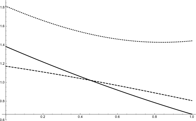
Refer to caption
Figure 4.2: Representation of the numerical solution of problem (4.8). The continuous line represents x⁡(t)x(t), the dashed line y⁡(t)y(t) and the dotted line ‖(t,x⁡(t),u⁡(t))‖\|(t,x(t),u(t))\|. Observe that the dotted line is always below two.

5 Multiplicity results

As we did in the case of admissible regions and solution regions, we present here a slightly modified definition of strict solution region [6].

Definition 5.1.

A solution region (R,(h,p))(R,(h,p)) is a strict CC-solution region of problem (1.1) if the following hold:

  1. (H0’)

    R̊t≠∅\mathring{R}_{t}\neq\emptyset for every t∈It\in I.

  2. (H4”)

    There exists "∈R+\varepsilon\in{\mdmathbb R}^{+} such that ∂h∂t​(t,x)+⟨∇xh​(t,x),f⁡(p⁡(t,x))⟩≤0\frac{\partial h}{\partial t}(t,x)+\left\langle\nabla_{x}h(t,x),f(p(t,x))\right\rangle\leq 0 for a.e. tt and every xx with (t,x)∈h−1​((,,,))(t,x)\in h^{-1}((-\varepsilon,0)). Also, ∂h∂t\frac{\partial h}{\partial t} and ∇xh\nabla_{x}h are locally Carathéodory in h−1​((,,,))h^{-1}((-\varepsilon,0)).

  3. (H5”)

    h⁡(a,u⁡(a))<0h(a,u(a))<0 or h⁡(a,u⁡(a))<h⁡(b,u⁡(b))h(a,u(a))<h(b,u(b)) for any u∈Bu\in B such that ‖u‖0≤C\|u\|_{0}\leq C.

Remark 5.2.

(H0’) is a stronger condition than (H0) and (H5”) than (H5). On the other hand, (H4”) complements (H4) by extending it to part of the interior of RR. Clearly, if h≥0h\geq 0, such as would be the case if it had been obtained by the construction in Theorem 2.10 or in the previous example, this condition would be vacuous.

Now we extend [6, Proposition 6.3] to the case of conditions (1.4) or (1.5). The proof is basically the same, but we include it for completeness.

Proposition 5.3.

Let f:I×Rn→Rnf:I\times{\mdmathbb R}^{n}\to{\mdmathbb R}^{n} be a Carathéodory function and (R,(h,p))(R,(h,p)) a strict solution region of problem (1.1). Assume uu is a solution of problem (1.1) such that (t,u⁡(t))∈R(t,u(t))\in R for every t∈It\in I. Then (t,u⁡(t))∈R̊(t,u(t))\in\mathring{R} for every t∈It\in I.

Proof.

We do the proof in the case of the case of conditions (1.4) or (1.5). Assume J:={t∈I:h⁡(t,u⁡(t))=0}≠∅J:=\{t\in I\ :\ h(t,u(t))=0\}\neq\emptyset. Observe that a∉Ja\not\in J. If that were the case, 0=h⁡(a,u⁡(a))<h⁡(b,u⁡(b))≤00=h(a,u(a))<h(b,u(b))\leq 0, which is a contradiction. Let r=min⁡J∈(a,b]r=\min J\in(a,b]. We have that h⁡(t,u⁡(t))<0h(t,u(t))<0 for t∈[0,r)t\in[0,r). Let "∈R+\varepsilon\in{\mdmathbb R}^{+} as in (H4”). Since uu and hh are continuous, there exist t1,t2∈[0,r)t_{1},t_{2}\in[0,r), t1<t2t_{1}<t_{2} such that h⁡(t1,u⁡(t1))<h⁡(t2,u⁡(t2))h(t_{1},u(t_{1}))<h(t_{2},u(t_{2})) and h⁡(t,u⁡(t))∈(−",0)h(t,u(t))\in(-\varepsilon,0) for all t∈[t1,t2]t\in[t_{1},t_{2}]. Using (H4”) we get

0<\displaystyle 0< h⁡(t2,u⁡(t2))−h⁡(t1,u⁡(t1))=∫t1t2dd⁡t​h​(t,u⁡(t))​d​t\displaystyle h(t_{2},u(t_{2}))-h(t_{1},u(t_{1}))=\int_{t_{1}}^{t_{2}}\frac{\operatorname{d}}{\operatorname{d}t}h(t,u(t))\operatorname{d}t
=\displaystyle= ∫t1t2(∂h∂t​(t,x)+⟨∇xh​(t,u⁡(t)),f⁡(p⁡(t,u⁡(t)))⟩)​d​t≤0,\displaystyle\int_{t_{1}}^{t_{2}}\left(\frac{\partial h}{\partial t}(t,x)+\left\langle\nabla_{x}h(t,u(t)),f(p(t,u(t)))\right\rangle\right)\operatorname{d}t\leq 0,

which is a contradiction and, hence, J=∅J=\emptyset and h⁡(t,u⁡(t))<0h(t,u(t))<0 for every t∈It\in I Since hh is continuous and R=h−1((−∞,0])R=h^{-1}((-\infty,0]), ∂R=h−1​(0)\partial R=h^{-1}(0), so (t,u⁡(t))∈R̊(t,u(t))\in\mathring{R} for every t∈It\in I. ∎

Remark 5.4.

The statement ‘(t,u⁡(t))∈R̊(t,u(t))\in\mathring{R} for every t∈It\in I’ in Proposition 5.3 is slightly stronger than the statement ‘u⁡(t)∈R̊tu(t)\in\mathring{R}_{t} for every t∈It\in I’ in [6, Proposition 6.3], but the proof in [6] also covers this case. It can be checked that

R̊⊂⋃t∈I({t}×R̊t),\mathring{R}\subset\bigcup_{t\in I}(\{t\}\times\mathring{R}_{t}),

but the reverse content is not in general true. In fact, �1​(⋃t∈I({t}×R̊t))\pi_{1}\left(\bigcup_{t\in I}(\{t\}\times\mathring{R}_{t})\right) might be connected while �1​(R̊)\pi_{1}(\mathring{R}) might be not.

Proposition 5.3 allows us to prove a variety of multiplicity results in a standard way through Fixed Point Index Theory (cf. [6, 15]).

6 Conclusions

As it was pointed out before, we have substituted the original condition

  • (H3’)

    pp is bounded and such that p⁡(t,x)=(t,x)p(t,x)=(t,x) for every (t,x)∈R(t,x)\in R and

    ⟨∇xh​(t,x),p2​(t,x)−x⟩<0​ for a. e. t and every x with (t,x)∈(I×Rn)\R.\left\langle\nabla_{x}h(t,x),p_{2}(t,x)-x\right\rangle<0\text{ for a.\,e. $t$ and every $x$ with $(t,x)\in(I\times{\mdmathbb R}^{n})\backslash R$.}

in the definition of admissible region [6] by the weaker version (H3). As a result we had to ask for (H6) to be satisfied in order to prove Propositions 4.4 and 4.8 and Theorems 4.5 and 4.9. The reason for this change was the need to prove de existence of admissible pairs associated to a given admissible function. Theorem 2.10 provides such a result and it may be possible to improve it by obtaining an admissible pair satisfying (H3’) instead of (H3).

Such a proof would not be devoid of difficulties. There are several ways to construct a 𝒞∞{\mathcal{C}}^{\infty} function ff that vanishes only on RR, for instance convolving the indicator function with a bump function, using a Whitney’s cover (see [16, Proposition 3.3.6], [17, Section 5.3] or [22]), etc. Furthermore, it seems possible to obtain such a function further satisfying that (∇xf)−1​({0})(\nabla_{x}f)^{-1}(\{0\}) is countable (in the case of a closed subset of R{\mdmathbb R} this is straightforward) although the topology of RR may play an important role in the construction.

Various approaches may be taken at this point. Analytic functions on R{\mdmathbb R} satisfy that, if non-constant, they cannot vanish on a set with accumulation points, a fact that could be relevant when we observe that, Whitney’s Extension Theorem [22, Theorem I] provides an extension that is analytic outside of the original domain of the function.

As said before, the topology of RR plays an important role. This is due to the following result.

Lemma 6.1.

Let f:Rn→[0,+∞)f:{\mdmathbb R}^{n}\to[0,+\infty) be differentiable. Let R:=f−1​({0})=RR:=f^{-1}(\{0\})=R. Let CC be a bounded connected component of Rn\R{\mdmathbb R}^{n}\backslash R. Then there exists x∈Cx\in C such that ∇f​(x)=0\nabla f(x)=0.

Proof.

Since CC is bounded, C¯\overline{C} is compact and, hence, being ff continuous, it reaches a maximum value in C¯\overline{C}. Since f>0f>0 in CC and ff is 00 in ∂C\partial C, the maximum is attained at some point x∈Cx\in C. Since ff differentiable in the open set CC we have that f′​(x)=0f^{\prime}(x)=0. ∎

Furthermore, any open set in Rn{\mdmathbb R}^{n} may have at most a countable number of connected components. This is due to the fact that Rn{\mdmathbb R}^{n} is a second countable topological space. This means that we have a lower bound for the number of zeros the gradient of a function f:Rn→[0,+∞)f:{\mdmathbb R}^{n}\to[0,+\infty) may have in f−1​(R+)f^{-1}({\mdmathbb R}^{+}).

The relation of critical points of a function with the connected components of the domain is also consequence of a basic result in Morse Theory known as the Morse inequalities [21, Theorem 5.2]. To be precise, it relates the topological invariants known as Betti numbers (the first of them being the number of connected components) to the number of the different types of non-degenerate singularities of the function. Thus, Morse Theory might shed light on our problem. We have the following well known results.

Theorem 6.2 ([19, Corollary 2.18]).

A non-degenerate critical point is isolated.

Theorem 6.3 ([19, Theorem 2.20] Existence of Morse functions).

Let MM be a closed mm-manifold and g∈𝒞∞​(Rn,R)g\in\mathcal{C}^{\infty}(\mdmathbb R^{n},\mdmathbb R). Then there exists a Morse function f∈𝒞∞​(Rn,R)f\in\mathcal{C}^{\infty}(\mdmathbb R^{n},\mdmathbb R) arbitrarily close to gg.

Since Morse functions have only non-degenerate critical points, they have at most a countable number of such points, making them another suitable approach to the problem.

Acknowledgements

The author would like to acknowledge his gratitude towards Professor Santiago Codesido for his help with the code for the computation of the numerical solution in the example, to Professor Marlène Frigon for her explanatory comments concerning her paper [6] and to Professors Rodrigo López Pouso and Ignacio Márquez Albés for their insightful advice regarding linear functionals defined by Lebesgue-Stieltjes integration.

References

  • [1] Benedetto, J.J., Czaja, W.: Integration and modern analysis. Birkhäuser Boston, Inc., Boston, MA (2009)
  • [2] Cabada, A., López Pouso, R.: Extremal solutions of strongly nonlinear discontinuous second-order equations with nonlinear functional boundary conditions. Nonlinear Analysis: Theory, Methods & Applications 42(8), 1377–1396 (2000)
  • [3] Cid, J.A., Tojo, F.A.F.: A Lipschitz condition along a transversal foliation implies local uniqueness for ODEs. Electron. J. Qual. Theory Differ. Equ. 13, 1–14 (2018)
  • [4] El Khattabi, N., Frigon, M., Ayyadi, N.: Multiple solutions of problems with nonlinear first-order differential operators. Journal of Fixed Point Theory and Applications 17(1), 23–42 (2015)
  • [5] Frigon, M.: Systems of first order differential inclusions with maximal monotone terms. Nonlinear Analysis: Theory, Methods & Applications 66(9), 2064–2077 (2007)
  • [6] Frigon, M.: Existence and Multiplicity Results for Systems of First-Order Differential Equations via the Method of Solution-Regions. Advanced Nonlinear Studies (2018)
  • [7] Frigon, M., Lotfipour, M.: Multiplicity results for systems of first order differential inclusions. J. Nonlinear Convex Anal 16, 1025–1040 (2015)
  • [8] Frigon, M., O’Regan, D.: Existence results for some initial and boundary value problems without growth restriction. Proc. Amer. Math. Soc. 123(1), 207–216 (1995)
  • [9] Frigon, M., O’Regan, D.: Nonlinear first-order initial and periodic problems in Banach spaces. Appl. Math. Lett. 10(4), 41–46 (1997)
  • [10] Gaines, R.E., Mawhin, J.L.: Ordinary differential equations with nonlinear boundary conditions. Journal of Differential Equations 26(2), 200–222 (1977)
  • [11] Gaines, R.E., Mawhin, J.L.: Coincidence degree and nonlinear differential equations, vol. 568. Springer (2006)
  • [12] Graef, J.R., Kong, L.: Existence of multiple periodic solutions for first order functional differential equations. Math. Comput. Modelling 54(11-12), 2962–2968 (2011)
  • [13] Granas, A., Dugundji, J.: Fixed point theory. Springer Verlag, New York (2003)
  • [14] Holmes, R.B.: A course on optimization and best approximation, vol. 257. Springer (2006)
  • [15] Infante, G., Pietramala, P., Tojo, F.A.F.: Non-trivial solutions of local and non-local Neumann boundary-value problems. Proceedings of the Royal Society of Edinburgh Section A: Mathematics 146(2), 337–369 (2016)
  • [16] Krantz, S., Parks, H.: A primer of real-analytic functions. Birkhauser Verlag (1992)
  • [17] Krantz, S.G., Parks, H.R.: The geometry of domains in space. Springer Science & Business Media (2012)
  • [18] López Pouso, R.: Nonordered discontinuous upper and lower solutions for first-order ordinary differential equations. Nonlinear Analysis: Theory, Methods & Applications 45(4), 391–406 (2001)
  • [19] Matsumoto, Y.: An introduction to Morse theory, vol. 208. American Mathematical Soc. (2002)
  • [20] Mawhin, J.: First order ordinary differential equations with several periodic solutions. Zeitschrift für angewandte Mathematik und Physik ZAMP 38(2), 257–265 (1987)
  • [21] Milnor, J.: Morse Theory. In: Annals of mathematics studies (1963)
  • [22] Whitney, H.: Analytic extensions of differentiable functions defined in closed sets. Trans. Amer. Math. Soc. 36(1), 63–89 (1934)