Vector polarizability of atomic state induced by a linearly polarized vortex beam: External control of magic, tune-out wavelengths, and heteronuclear spin oscillations

In recent years, laser trapping and cooling of neutral atoms have attracted significant attention to the experimentalists and achieved as an established technique in high precision spectroscopic measurements Champenois2004; Chou2010; Ludlow2015. Along with neutral atoms, optical dipole trappings of ions have recently surged interest in ultra-cold physics Laupretre2019; Schmidt2018; Lambrecht2017; Schaetz2017. However, mechanism of the trapping by optical means inevitably produces the Stark shifts in the atomic energy levels and influences the fidelity of the precision measurements. Magic wavelengths are the unique wavelengths of the external laser beam for which the differential ac-Stark shift of an atomic transition effectively vanishes. Therefore, the impediment in precise spectroscopic measurements can be eliminated almost entirely if the atoms are confined at the predetermined magic wavelengths of the laser beam. The light at magic wavelengths have significant applications in atom optics, such as atomic interferometers Biedermann2015, atomic clocks Margolis2009; Rosenbusch2009; Nicholson2015, and atomic magnetometers Dong2015, etc.

Determinations of magic wavelengths for an atomic transition depend mainly on how accurately the frequency-dependent valence polarizability (POL) values of the atomic Zeeman sub-levels are calculated. The valence POL consists of three components, scalar POL ($\alpha_{V}^{0}$), vector POL ($\alpha_{V}^{1}$), and tensor POL ($\alpha_{V}^{2}$) Flambaum2008; Arora2007; Lacroute2012; Arora2012. In general, POL is defined in terms of an off-resonant electric dipole interaction between the atom and its trapping light. The vector POL, which yields the energy shift among the Zeeman sublevels, arises usually due to a circularly polarized light Flambaum2008; Bhowmik2018; Das2020. It is one of the non-magnetic field sources to remove Zeeman degeneracy and becomes very significant in the evaluation of magic wavelengths for cases such as ”knob” to adjust an optical trap Kim2013.

In this work, we theoretically develop and demonstrate that a linearly polarized focused vortex (LP-FV) beam can naturally produce vector part of the dynamic POL when it interacts with cold atoms or ions. The vector part is certainly not a component of dynamic POL for a linearly polarized Gaussian or paraxial vortex beam. The distinctive feature of the vortex beam is that in addition to the spin angular momentum associated with the polarization, it has orbital angular momentum (OAM) which arises due to the helical phase front of the beam Allen1992; Babiker2002; Lembessis2011; Afanasev2013; Mondal2014; Bhowmik2016; Schmiegelow2016; Bhowmik_JPC_2018; Romero2012; SDas2020; Quinteiro2020. We find that the origin of the vector POL comes from the prolific artifacts of the spin-orbit coupling of LP-FV beam satisfying the conservation of the total angular momentum of the beam during the interaction-process. Also, this vector POL creates a fictitious magnetic field Kien2013 when it interacts with an atomic system. This fictitious magnetic field interrogates, manipulates, and traps an atom or ion independently Albrecht2016 or in conjunction with the real magnetic field Schneeweiss2014. Further, this fabricated field provides a unique opportunity for exploring spin-dynamics in the form of coherent spin oscillations Stenger1998; Chang2004; Chang2005; Klempt2009 in the ultra-cold spinor quantum gas. This has been the subject of intensive theoretical and experimental research due to its high controllability Kurn2013.

The primary objective of the present work is to visualize the effect of vector POL, originated due to the spin-orbit coupling of the LP-FV beam, in the clock transitions and clock states. We apply our theory to calculate the dynamic POL values of the fine-structure states, $5S_{\frac{1}{2}}$, $4D_{\frac{3}{2}}$, and $4D_{\frac{5}{2}}$ of ⁸⁷Sr⁺. Singly ionized strontium is an excellent candidate for optical frequency standard, quantum information, and quantum storage Akerman2015; Shapira2018. As the spin-orbit coupling of LP-FV beam varies with the choice of OAM and focusing angle of the lens, we quantitatively show the effects of these parameters on the magic wavelengths for $5S_{\frac{1}{2}}\rightarrow 4D_{\frac{3}{2},\frac{5}{2}}$ transitions and tune-out wavelengths (where the dynamic POL value becomes zero LeBlanc2007; Wang2016). These quantifications will be important for the experimentalists to choose the parameters of the vortex beams used for trapping Kim2013; Albrecht2016. In order to manifest the impact of the vector POL, we compare the calculated magic and tune-out wavelengths induced from the LP-FV beam with the corresponding wavelengths induced from a linearly polarized Gaussian beam. Moreover, as an important application, we investigate how the fictitious magnetic field, originated from the vector POl, can control the coherent heteronuclear spin oscillations in a spin-1 mixture of ⁸⁷Rb and ²³Na atoms with influences from both linear and quadratic Zeeman shifts.

According to the time-independent second-order perturbation theory Mitroy2010, the ac-Stark shift of an atomic state in an external oscillating electric field $\mathcal{E}(\omega)$ is expressed by $\Delta F(\omega)=-\frac{1}{2}\alpha^{T}(\omega)\mathcal{E}^{2}$, where $\alpha^{T}(\omega)$ is the total dynamic POL of the atomic state at frequency $\omega$ and $\mathcal{E}$ is the magnitude of the external electric field. For a single-valence atom with a valence electron in the $v$th orbital, the total dynamic POL can be written as $\alpha^{T}(\omega)=\alpha^{C}(\omega)+\alpha^{VC}(\omega)+\alpha^{V}(\omega)$. Here $\alpha^{C}(\omega)$ is the frequency-dependent core POL of the ionic core obtained by removing the valence electron. $\alpha^{VC}(\omega)$ gives a correction Dutta2015 to the core POL due to the presence of the valence electron, and it is considered as $\omega$-independent in the present work. $\alpha^{V}(\omega)$ is the valence POL of the single-valence state. $\alpha^{C}$ and $\alpha^{VC}$ provide small contributions to $\alpha^{T}$ compared to $\alpha^{V}$, and they are computed approximately using lower-order many-body perturbation theory Mitroy2010; Ghosh1993; Dutta2020.

Now, we evaluate $\alpha^{V}(\omega)$ in the presence of an external LP-FV beam. As Laguerre-Gaussian (LG) beam is a well-established example of a vortex beam, initially, we assume a paraxial form of linearly polarized coherent LG beam without any off-axis node and propagates along the $z$-axis. The field is expressed as Mondal2014 $\bm{{{\mathcal{E}_{i}}}}(\rho,\phi,z,t)=\mathcal{E}_{i}(t)\left({{\sqrt{2}\rho}/{w_{0}}}\right)^{\lvert l\rvert}e^{i(l\phi+k_{0}z)}\bm{\hat{\textbf{x}}}$. Here $k_{0}$ is the wave number of the free space, $w_{0}$ is the waist-size and $l$ is OAM of the beam. We consider that this paraxial LG beam is focused by passing through an objective (lens) with a high numerical aperture (NA) Bhowmik2016. Then this focused LG beam interacts with a cold atom or ion whose de Broglie wavelength is large enough to experience the intensity variation of this beam. In order to take a full advantage of the high NA of the lens, we assume that $w_{0}$ overfills the entrance aperture radius. According to the Kirchhoff’s approximation in diffraction theory Richards1959; Boivin1965, the consequent components of the spin-orbit coupled LP-FV beam can be expressed as

Here $\mathcal{E}_{x}$, $\mathcal{E}_{y}$, and $\mathcal{E}_{z}$ are the $x$-, $y$-, and $z$- components of the electric field, respectively. The amplitude of the focused electric field is $\mathcal{E}_{0}=\dfrac{\pi f}{\lambda}T\mathcal{E}_{i}$, where $\mathcal{E}_{i}$ is the amplitude of the incident electric field, $T$ is the transmission coefficient of the objective, and $f$ is its focal length related to $\rho$ by $\rho=f\sin\theta$ (Abbe sine condition). The coefficients $u_{l+m}$, where $m$ takes the values 0, $\pm 1$, and $\pm 2$ in the above expression, depend on the focusing angle of NA ($\vartheta_{m}$) following the relation Zhao2007 $u_{l+m}(\rho,z)=\int_{0}^{\vartheta_{m}}d\vartheta\left({\dfrac{\sqrt{2}\rho}{w_{0}}}\right)^{\lvert l\rvert}\sin\vartheta\sqrt{\cos\vartheta}g_{\lvert m\rvert}(\vartheta)J_{l+m}(k\rho\sin\vartheta)e^{ikz\cos\vartheta}.$ Here $J_{l+m}(k\rho\sin\vartheta)$ represents cylindrical Bessel function and $k=\mu k_{0}$ with $\mu$ as the refractive index of the lens medium. $g_{|m|}(\vartheta)$ are the angular functions with $g_{0}(\vartheta)=1+\cos\vartheta$, $g_{1}(\vartheta)=\sin\vartheta$, and $g_{2}(\vartheta)=1-\cos\vartheta$.

Now, let us discuss about Eq. (II) in detail. Linearly polarized light can be considered as the superposition of left ($\beta=+1$) and right ($\beta=-1$) circularly polarized beams. Because of the focusing and the diffraction from the edges of the aperture, each circularly polarized light ($\beta=\pm 1$) can be decomposed into three sets of local polarizations ($\pm 1$, $\mp 1$, and polarization along z-axis) Bhowmik2016. Among these three sets of local polarizations, the first set has equal amplitude ($u_{l}$) for $\pm 1$ local polarizations. Therefore, after passing through the focusing lens, the superposition of these local polarizations results linearly polarized beam with the OAM similar to the OAM of the incident beam. However, in the case of second set, different field amplitudes, $u_{l+2}$ and $u_{l-2}$, are generated with two different local polarizations ($-1$ and $+1$, respectively) and topological charges ($l+2$ and $l-2$, respectively, to conserve total angular momentum) after passing through the lens. Therefore, the field gains two opposite circular polarizations with different amplitudes and creates the vector part of valence POL in interaction with an atom or ion. The third set yields $u_{l+1}$ and $u_{l-1}$ fields with topological charges, $l+1$ and $l-1$, respectively. However, both these fields are polarized along the $z$- direction, which is another interesting manifestation of focusing beam. Nevertheless, using LP-FV beam presented in Eq. (II), $\alpha^{V}(\omega)$ of the atomic state can be presented by

Here the coefficients $C_{i}$s are expressed in the following forms:

where $J_{V}$ and $M_{J_{V}}$ are the total angular momentum and its magnetic component for the single-valence atomic state $|\Phi_{V}\rangle$. The mathematical expressions of the scalar, vector, tensor, and consequently the valence POL at the fine- and hyperfine-structure levels are presented in the Appendix. The calculation of $\alpha^{V}(\omega)$ Mitroy2010; Bhowmik2018 of an atomic state directly depends on different combinations of the integrals $u_{l+m}$. These integrals can be altered with the various choices of the topological charges of the incident LG beam and the NA of the objective. As a consequence, the total POL values of the atomic states and the magic wavelengths for the transitions among them can be tuned externally using different parameters of the beam.

As the electron-correlation most significantly affects $\alpha^{V}(\omega)$ part of the dynamic POL due to the loosely bound valence electron, the accurate estimations of the scalar, vector, and tensor components of $\alpha^{V}(\omega)$ for the different states require correlation exhaustive many-body calculations Lindgren1985; Bishop1987; Lindgren1986; Lindgren_1985; Bartlett2007; Dutta2016; Bhowmik2017; Bhowmik2017b; Das2018 with a sophisticated numerical approach (see Appendix for the details of computations). To have a quantitative analysis of the effect of OAM of LP-FV beam on the total vector POL ($C_{1}\alpha_{V}^{1}(\omega)$) of an atomic state, we show variations of $C_{1}\alpha_{V}^{1}(\omega)$ with frequency for $5S_{\frac{1}{2}}(+1/2)$ and $4D_{\frac{3}{2},\frac{5}{2}}(+1/2)$ states of ⁸⁷Sr⁺ in Fig. 1 ($M_{J}=-\frac{1}{2}$ provides opposite sign to $C_{1}\alpha_{V}^{1}(\omega)$). The fine-structure states $5S_{\frac{1}{2}}$, $4D_{\frac{3}{2}}$, and $4D_{\frac{5}{2}}$ are indicated by $5S1$, $4D3$, and $4D5$, respectively in this figure and the next two figures of this paper. Here LP-FV beam has either OAM=+1 or +2 with focusing angle of 60^∘. Although the effect of variation of focusing angle to $C_{1}\alpha_{V}^{1}(\omega)$ is marginal, it is significant to the total scalar and tensor POL values, and consequently to the total POL values. The peak values of $C_{1}\alpha_{V}^{1}(\omega)$ occur at resonance frequencies: 0.11 a.u. for $5S_{\frac{1}{2}}$ state; around 0.045 a.u and 0.21 a.u. for $4D_{\frac{3}{2},\frac{5}{2}}$ states, respectively. However, many small scale structures in $C_{1}\alpha_{V}^{1}(\omega)$ profiles of $4D_{\frac{3}{2},\frac{5}{2}}$ states appear due to multiple number of resonance transitions at around 0.25 a.u. to 0.30 a.u.

It can be seen from the graphs that OAM=+1 always produces higher peak value of $C_{1}\alpha_{V}^{1}(\omega)$ compared to OAM=+2. This is because of the stronger spin-orbit coupling for OAM=+1 compared to OAM=+2. Also, the magnitude of the peak value of $C_{1}\alpha_{V}^{1}(\omega)$ is higher for larger $M_{J}$ for a fixed value of $J$, which is obvious from the expression of $C_{1}$.

Fig. 2 displays profiles of $\alpha^{T}$ for $5S_{\frac{1}{2}}$ and $4D_{\frac{3}{2},\frac{5}{2}}$ states of ⁸⁷Sr⁺ at 60^∘ focusing angle for LP-FV beam with OAM=+1. However, it should be mentioned that focusing angle does affect $\alpha^{T}$ values at various frequencies of the beam. Fig. 2 shows a number of intersection points between $\alpha^{T}$ profiles of the multiplets of $5S_{\frac{1}{2}}$ and $4D_{\frac{3}{2},\frac{5}{2}}$ states. These intersection points indicate the magic wavelengths at which the differential ac-Stark shift of the associated clock transition states vanishes. We observe five sets (Set-1 to Set-5) of magic wavelengths for $5S_{\frac{1}{2}}\rightarrow 4D_{\frac{3}{2},\frac{5}{2}}$ clock transitions within the frequency span (from the near-infrared to the ultra-violet regions) as shown in the figures (see Appendix). This is true for all the magnetic sublevels involed in the transitions. However, the infrared magic wavelengths (fall under Set-1 and Set-2) are the most important to trap ⁸⁷Sr⁺ ion due to relatively large $\alpha^{T}$ values and support the red-detuned trapping scheme useful for frequency standard experiment. We find that the magic wavelengths for the clock transitions at Set-1 are maximally affected by the spin-orbit coupling of the beam. For $5S_{\frac{1}{2}}\rightarrow 4D_{\frac{5}{2}}(+3/2)$ transition, the magic wavelength at Set-1 is 1793.83 nm for either linearly polarized paraxial LG beam or Gaussian beam. The results are same as OAM of the paraxial light does not affect the electronic motion of an cold atom or ion (which is below its recoil limit) at the dipole transition level Bhowmik2018; Mondal2014. However, we observe that for OAM=+1 and +2 of LP-FV beam the magic wavelengths of $5S_{\frac{1}{2}}\rightarrow 4D_{\frac{5}{2}}(+3/2)$ transition at Set-1 can be varied upto -20% and -15%, respectively, compared to the corresponding magic wavelength of Gaussian beam.

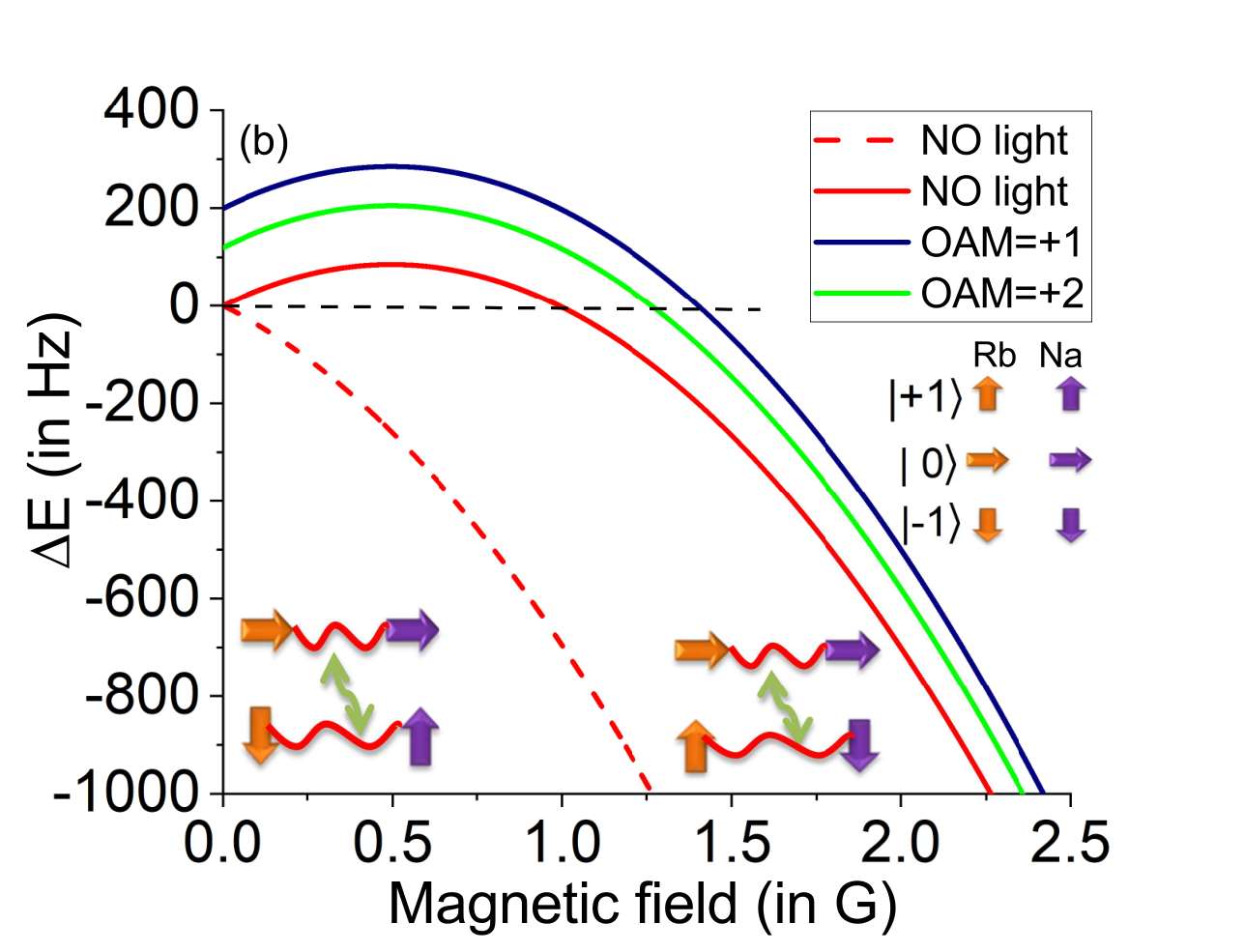
Fig. 3 illustrates wavelength dependence on $\alpha^{T}$ for the clock transition state $4D_{\frac{3}{2}}$ of ⁸⁷Sr⁺ due to the external field of LP-FV beam with OAM=+1 and +2, focused at angle of 60^∘, and linearly polarized paraxial Gaussian beam. As the beam is linearly polarized, the vector component does not arise in $\alpha^{T}$ for the Gaussian beam. Therefore, the tune-out wavelengths for $4D_{\frac{3}{2}}(M_{J}=\pm 1/2)$ and $4D_{\frac{3}{2}}(M_{J}=\pm 3/2)$ states are degenerated with respect to the sign of $M_{J}$ and their values are 507.83 nm and 744.12 nm, respectively. These degeneracies are lifted for LP-FV beam. This leads to splitting of the tune-out wavelengths for the oppositely signed $M_{J}$-levels with respect to the corresponding tune-out wavelengths for the linearly polarized Gaussian beam. The figure shows that non-zero OAM of the LP-FV beam causes red-shifting and blue-shifting of the tune-out wavelengths with respect to the tune-out wavelengths of the Gaussian beam for $M_{J}=|\frac{1}{2}|$ and $M_{J}=|\frac{3}{2}|$, respectively. The comparison of panels (a) and (b) of Fig. 3 reveals that the separation between the tune-out wavelengths corresponding to $+M_{J}$ and $-M_{J}$ of a particular value of $M_{J}$ decreases with the increasing OAM of the beam. This also indicates the decreasing strength of the spin-orbit coupling with the increasing OAM of the LP-FV beam

We also gauge the effect of the vector POL arising from LP-FV beam by considering a heteronuclear spin-1 mixture of ⁸⁷Rb and ²³Na atoms with spin states $|M_{F_{V1}}\rangle$ and $|M_{F_{V2}}\rangle$, respectively, of $F_{V1}=F_{V2}=1$ hyperfine levels of their respective ground states $5S_{\frac{1}{2}}$ and $3S_{\frac{1}{2}}$. Here, we show how their coherent spin oscillations can be controlled by the fictitious magnetic field generated from the vector POL due to LP-FV beam. We calculate the total magnetic energy $E^{|M_{F_{V1}},M_{F_{V2}}\rangle}(B)$ (from the Breit-Rabi formula Vanier1988) associated with $|M_{F_{V1}},M_{F_{V2}}\rangle$ state, where $B$ is the externally applied magnetic field. In this example, we start with $|0,0\rangle$ mixture of ⁸⁷Rb and ²³Na atoms. Therefore, we have only two types of spin-changing transition process at $F_{V}=1$ level conserving the total magnetization: $|0,0\rangle\leftrightarrow|-1,1\rangle$ and $|0,0\rangle\leftrightarrow|1,-1\rangle$. In the presence of a laser beam, the magnitudes of the frequency-dependent Stark-shifts for both the atoms largely depend on the positions of the $D$-line transitions, which are close to 590 nm and 790 nm for the ²³Na and ⁸⁷Rb atoms, respectively. Therefore, if a light beam of wavelength nearly 790 nm is used, it can make the Stark-shift essentially species-selective for ⁸⁷Rb, but mostly transparent for ²³Na. The dynamic polarizability for the state $|5S_{1/2},F_{V}=1,M_{F_{V}}=0,\pm 1\rangle$ of ⁸⁷Rb is depicted in Fig 4(a) for 786-794 nm. Here a LP-FV beam with intensity $10$ W/cm² and both OAM=+1, +2 are employed to selectively dresses the energy levels of ⁸⁷Rb near 790.14nm wavelength, which is the tune-out wavelength for $M_{F_{V}}=0$ state. The figure shows that the Stark shift for $M_{F_{V}}=\pm 1$ is larger for OAM=+1 compared to OAM=+2 at the wavelength 790.14 nm.

Without the LP-FV beam, the total Zeeman energy difference of the process $|0,0\rangle\leftrightarrow|-1,1\rangle$ is indicated by $\Delta E^{-}(B)=E^{|0,0\rangle}-E^{|-1,1\rangle}$ and of the process $|0,0\rangle\leftrightarrow|1,-1\rangle$ is indicated by $\Delta E^{+}(B)=E^{|0,0\rangle}-E^{|1,-1\rangle}$. These Zeeman energy differences of the heteronuclear spin-oscillations include contributions of both the linear and quadratic Zeeman shifts Zhang2005. Since the heteronuclear spin oscillation can only occur near $\Delta E^{\pm}(B)=0$ Li2015, Fig. 4(b) suggests that only the oscillation $|0,0\rangle\leftrightarrow|1,-1\rangle$ is possible at the magnetic field 0.99 G. The other oscillation, $|0,0\rangle\leftrightarrow|-1,1\rangle$, is strongly suppressed at this magnetic field. Now, taking into account the light shift by the LP-FV beam on ⁸⁷Rb atom at the wavelength 790.14 nm, the total Zeeman energy difference of the allowed process is modified to $\Delta E^{+}(B)=(E^{|0,0\rangle}-E^{|1,-1\rangle})+[\delta E_{l}(M_{F_{V}}=0)-\delta E_{l}(M_{F_{V}}=1)]$, where $\delta E_{l}$ is the light shift. In Fig 4(b), we find that $\Delta E^{+}(B)$ becomes zero at the magnetic fields 1.40 G and 1.26 G for OAM=+1 and +2, respectively, of LP-FV beam. Therefore, the external magnetic field that is required for $|0,0\rangle\leftrightarrow|1,-1\rangle$ transition with $\Delta E^{+}(B)=0$ to take place is changed significantly due to the presence of the LP-FV beam, which accounts the fictitious magnetic field generated by the vector polarizability. This is purely a manifestation of the vector light shift arises from the spin-orbit coupling of the beam. Also, the spin oscillations process of the heteronuclear spin-1 mixture of ⁸⁷Rb and ²³Na can be controlled externally by changing focusing angle and OAM of LP-FV beam. This process will be very useful for recent experiment using spherical-quadrupole magnetic trap Fang2019.

In summary, we have developed a theoretical formalism to calculate the dynamic POL of an atomic state in the external field of a LP-FV beam. We have demonstrated how the OAM and focusing angle of the beam induce the spin-orbit coupling in the beam, which in turn produces vector polarizability in the atomic state even for linearly polarized light. The fine tuning of magic wavelengths for the clock transitions $5S_{\frac{1}{2}}\rightarrow 4D_{\frac{3}{2},\frac{5}{2}}$ of ⁸⁷Sr⁺ ion are demonstrated by controlling OAM and focusing parameters of LP-FV beam (details are in the Appendix). The vector POL values presented in this paper can be verified experimentally by stimulated Raman spectroscopy Hu2018 or by measuring the tune-out wavelengths for the magnetic sublevels of same multiplets Schmidt2016; Trubko2017. Moreover, we develop a controlling mechanism of heteronuclear spin oscillations of spin-1 mixture of ⁸⁷Rb and ²³Na atoms with the fictitious magnetic field generated by LP-FV beam. This mechanism can be used to tune the heteronuclear spin dynamics Li2020 and generate entanglement between distinguishable atoms Shi2006. We believe that the present theoretical development will give an additional flexibility in the spin-changing interaction process of other multi-species spinor condensates.

A.B. acknowledges Arghya Das for helpful discussions.

In this Appendix, we augment the main text with further details. In section A, we present a brief mathematical description of the scalar, vector, and tensor polarizabilities of a single-valence atomic state at the fine-structure and hyperfine levels. In section B, we show the numerical procedure to calculate the dynamic polarizabilities of ⁸⁷Sr⁺ and ⁸⁷Rb. In this Section, we also include the details of the Zeeman energy difference that leads the spin oscillation processes of the spin-1 mixture ⁸⁷Rb and ²³Na atoms. In section C, we tabulate a list of magic wavelengths and the corresponding vector and total polarizabilities for the clock transitions $5S_{\frac{1}{2}}\rightarrow 4D_{\frac{3}{2},\frac{5}{2}}$ of ⁸⁷Sr⁺ ion.

References

- (1) C. Champenois, M. Houssin, C. Lisowski,M. Knoop, G. Hagel, M. Vedel, and F. Vedel, Phys. Lett. A 331, 298 (2004).
- (2) C. W. Chou, D. B. Hume, J. C. J. Koelemeij, D. J. Wineland, and T. Rosenband, Phys. Rev. Lett. 104, 070802 (2010).
- (3) A. D. Ludlow, M. M. Boyd, J. Ye, E. Peik, and P. O. Schmidt, Rev. Mod. Phys. 87, 637 (2015).
- (4) T. Lauprêtre, R. B. Linnet, I. D. Leroux, H. Landa, A. Dantan, and M. Drewsen, Phys. Rev. A 99, 031401(R) (2019).
- (5) J. Schmidt, A. Lambrecht, P. Weckesser, M. Debatin, L. Karpa, and T. Schaetz, Phys. Rev. X 8, 021028 (2018).
- (6) A. Lambrecht, J. Schmidt, P. Weckesser, M. Debatin, L. Karpa, and T. Schaetz, Nat. Photonics 11, 704 (2017).
- (7) T. Schaetz, J. Phys. B: At. Mol. Opt. Phys. 50, 102001 (2017).
- (8) G. W. Biedermann, X. Wu, L. Deslauriers, S. Roy, C. Mahadeswaraswamy, and M. A. Kasevich, Phys. Rev. A 91, 033629 (2015).
- (9) H. S. Margolis, J. Phys. B 42, 154017 (2009).
- (10) T. Nicholson, S. Campbell, R. Hutson, G. Marti, B. Bloom, R. McNally, W. Zhang, M. Barrett, M. Safronova, G. Strouse et al., Nat. Commun. 6, 6896 (2015).
- (11) P. Rosenbusch, S. Ghezali, V. A. Dzuba, V. V. Flambaum, K. Beloy, and A. Derevianko, Phys. Rev. A 79, 013404 (2009).
- (12) R. C. Dong, R. Wei, Y. B. Du, F. Zou, J. D. Lin, and Y. Z. Wang, Appl. Phys. Lett. 106, 152402 (2015).
- (13) B. Arora, M. S. Safronova, and C. W. Clark, Phys. Rev. A 76, 052509 (2007).
- (14) C. Lacroûte, K. S. Choi ,A. Goban, D. J. Alton, D. Ding, N. P. Stern, H. J. Kimble, New J. Phys. 14, 023056 (2012).
- (15) B. Arora and B. K. Sahoo, Phys. Rev. A 86, 033416 (2012).
- (16) V. V. Flambaum, V. A. Dzuba, and A. Derevianko, Phys. Rev. Lett. 101, 220801 (2008).
- (17) A. Bhowmik, N. N. Dutta, and S. Majumder, Phys. Rev. A 97, 022511 (2018).
- (18) A. Das, A. Bhowmik, N. N. Dutta, and S. Majumder, Phys. Rev. A 102, 012801 (2020).
- (19) H Kim, H S Han, and D. Cho, Phys. Rev. Letts., 111, 243004 (2013)
- (20) L. Allen, M. W. Beijersbergen, R. J. C. Spreeuw, and J. P. Woerdman, Phys. Rev. A 45, 8185 (1992).
- (21) P. K. Mondal, B. Deb, S. Majumder, Phys. Rev. A 89, 063418 (2014).
- (22) A. Bhowmik, P. K. Mondal, S. Majumder, and B. Deb, Phys. Rev. A 93, 063852 (2016).
- (23) C. T. Schmiegelow, J. Schulz, H. Kaufmann, T. Ruster, U. G. Poschinger, and F. Schmidt-Kaler, Nature Communications 7, 12998 (2016).
- (24) A. Bhowmik and S. Majumder, J. Phys. Commun. 2, 125001 (2018).
- (25) M. Babiker, C. R. Bennett, D. L. Andrews, and L. C. D. Romero, Phys. Rev. Lett. 89, 143601 (2002).
- (26) V. E. Lembessis, D. Ellinas, and M. Babiker, Phys. Rev. A 84, 043422 (2011).
- (27) A. Afanasev, C. E. Carlson, and A. Mukherjee, Phys. Rev. A 88, 033841 (2013).
- (28) J. Romero, D. Giovannini, S. Franke-Arnold, S. M. Barnett, and M. J. Padgett, Phys. Rev. A 86, 012334 (2012).
- (29) S. Das, A. Bhowmik, K. Mukherjee, S. Majumder, J. Phys. B: At. Mol. Opt. Phys. 53, 025302 (2020).
- (30) G. F. Quinteiro, C. T. Schmiegelow, F. Schmidt-Kaler, arXiv:2004.00040
- (31) F. L. Kien, P. Schneeweiss, and A. Rauschenbeute, Eur. Phys. J. D 67 92 (2013).
- (32) B. Albrecht, Y. Meng, C. Clausen, A. Dareau, P. Schneeweiss, and A. Rauschenbeutel, Phys. Rev. A, 94, 061401(R) (2016).
- (33) P. Schneeweiss, F. L. Kien, and A. Rauschenbeutel, New J. Phys., 16, 013014 (2014).
- (34) J. Stenger, S. Inouye, D. M. Stampe-Kurn, H. J. Miesner, A. P. Chikkatur, and W. Ketterle, Nature 396, 345 (1998).
- (35) M. -S. Chang, C. D. Hamley, M. D. Barrett, J. A. Sauer, K. M. Fortier, W. Zhang, L. You, and M. S. Chapman, Phys. Rev. Lett. 92, 140403 (2004).
- (36) M. -S. Chang, Q. S. Qin, W. X. Zhang, L. You, and M. S. Chapman, Nat. Phys. 1, 111 (2005).
- (37) C. Klempt, O. Topic, G. Gebreyesus, M. Scherer, T. Henninger, P. Hyllus, W. Ertmer, L. Santos, and J. J. Arlt, Phys. Rev. Lett. 103, 195302 (2009).
- (38) D. M. Stamper-Kurn and M. Ueda, Rev. Mod. Phys. 85, 1191 (2013).
- (39) N. Akerman, N. Navon, S. Kotler, Y. Glickman, and R. Ozeri, New J. of Phys. 17, 113060 (2015).
- (40) Y. Shapira, R. Shaniv, T. Manovitz, N. Akerman, and R. Ozeri, Phys. Rev. Lett. 121, 180502 (2018).
- (41) L. J. LeBlanc and J. H. Thywissen, Phys. Rev. A 75,053612 (2007).
- (42) X. Wang, J. Jiang, L. -Y. Xie, D. -H. Zhang, and C. -Z. Dong Phys. Rev. A 94, 052510 (2016).
- (43) J. Mitroy, M. S. Safronova, and C. W. Clark, J. Phys. B: At. Mol. Opt. Phys. 43, 202001 (2010).
- (44) N. N. Dutta, S. Roy, and P. C. Deshmukh, Phys. Rev. A 92, 052510 (2015).
- (45) T. K. Ghosh, A. K. Das, M. Castro, S. Canuto, and P. K. Mukherjee, Phys. Rev. A 48, 2686 (1993).
- (46) N. N. Dutta, Chem. Phys. Lett. 758, 137911 (2020).
- (47) B. Richards and E. Wolf, Proc. R. Soc. London, Ser. A 253, 358 (1959).
- (48) A. Boivin and E. Wolf, Phys. Rev. 138, B1561 (1965).
- (49) Y. Zhao, J. S. Edgar, G. D. M. Jeffries, D. McGloin, and D. T. Chiu , Phys. Rev. Lett. 99, 073901 (2007).
- (50) I. Lindgren and J. Morrison, Atomic Many-body Theory, ed. G. E. Lambropoulos and H. Walther(3rd ed.; Berlin: Springer),3 (1985).
- (51) R. F. Bishop, and H. G. K?ummel, Physics Today March 40, 52 (1987).
- (52) I. Lindgren, and J. Morrison, Atomic Many-Body Theory, (Springer, 1986).
- (53) I. Lindgren, Phys. Rev. A 31, 1273 (1985).
- (54) R. J. Bartlett and M. Musial, Reviews of Modern Physics 79, 291 (2007).
- (55) N. N. Dutta and S. Majumder, Indian Journal of Physics 90, 373 (2016).
- (56) A. Bhowmik, N. N. Dutta, and S. Roy, Astrophys. J.836, 125 (2017).
- (57) A. Bhowmik, S. Roy, N. N. Dutta, and S. Majumder, J. Phys. B: At. Mol. Opt. Phys. 50, 125005 (2017).
- (58) A. Das, A. Bhowmik, N. N. Dutta, and S. Majumder, J. Phys. B: At. Mol. Opt. Phys. 51, 025001 (2018).
- (59) J. Vanier and C. Audoin, The Quantum Physics of Atomic Frequency Standards (Hilger, Philadelphia, 1988).
- (60) W. X. Zhang, D. L. Zhou, M. S. Chang, M. S. Chapman, and L. You, Phys. Rev. A 72, 013602 (2005).
- (61) X. Li, B. Zhu, X. He, F. Wang, M. Guo, Z. Xu, S. Zhang, and D. Wang, Phys. Rev. Lett. 114, 255301 (2015).
- (62) F. Fang, S. Wu, A. Smull, J. A. Isaacs, Y. Wang, C. H. Greene, and D. M. Stamper-Kurn, Phys. Rev. A 101, 012703 (2019).
- (63) Q. -Q. Hu, C. Freier, Y. Sun, B. Leykauf, V. Schkolnik, J. Yang, M. Krutzik, and A. Peters, Phys. Rev. A 97, 013424 (2018).
- (64) F. Schmidt, D. Mayer, M. Hohmann, T. Lausch, F. Kindermann, and A. Widera1, Phys. Rev. A 93, 022507 (2016).
- (65) R. Trubko, M. D. Gregoire, W. F. Holmgren, and A. D. Cronin, Phys. Rev. A 95, 052507 (2017).
- (66) L. Li, B. Zhu, B. Lu, S. Zhang, and D. Wang, Phys. Rev. A 101, 053611 (2020).
- (67) Y. Shi and Q. Niu, Phys. Rev. Lett. 96, 140401 (2006).
- (68) K. Beloy, Theory of the ac stark effect on the atomic hyperfine structure and applications to microwave atomic clocks, Doctoral dissertation, University of Nevada, Reno, USA, 2009.
- (69) V. A. Dzuba, V. V. Flambaum, K. Beloy, and A. Derevianko, Phys. Rev. A 82, 062513 (2010).
- (70) S. Biswas, A. Das, A. Bhowmik, and S. Majumder, Mon. Not. R. Astron. Soc. 477, 5605 (2018).
- (71) A. Kramida, Y. Ralchenko, J. Reader, and NIST ASD Team (2019). NIST Atomic Spectra Database (ver. 5.7.1), [Online]. Available: https://physics.nist.gov/asd [2020, October 26].
- (72) W. R. Johnson, Z. W. Liu, and J. Sapirstein, At. Data Nucl. Data Tables 64, 279 (1996).
- (73) U. I. Safronova, Phys. Rev. A 82, 022504 (2010).
- (74) E. Arimondo, M. Inguscio, and P. Violino, Rev. Mod. Phys. 49, 31 (1977).
- (75) T. Kuga, Y. Torii, N. Shiokawa, and T. Hirano, Phys. Rev. Lett. 78, 4713 (1997).
- (76) S. A. Kennedy, G. W. Biedermann, J. T. Farrar, T. G. Akin, S. P. Krzyzewski, and E. R. I. Abraham, Optics Communications 321, 110 (2014).
- (77) J. Arlt, K. Dholakia, J. Soneson and E. M. Wright Physical Review A 63, 063602 (2001).
- (78) E. M. Wright, J. Arlt, and K. Dholakia, Phys. Rev. A 63, 013608 (2000).