State Estimation in Water Distribution Networks through a New Successive Linear Approximation

In this section, we introduce the modeling of WDNs.

Classical state estimation problems are typically presented as

where ${\bm{\xi}}$ is the unknown variable, vector ${\bm{y}}$ includes all measured quantities, the $\bm{g}(\bm{\xi})$ is the model of system including nonlinear functions, and the $\bm{\epsilon}$ represents error between true model and measured values via sensors. As we mentioned in Section I, it is impossible to measure flows and pressures in the entire WDN, except for key locations. Hence, $\bm{\xi}$ can be a vector collecting all unknown variables and defined as

where $\bm{h}^{\mathrm{J}}$, $\bm{h}^{\mathrm{R}}$, and $\bm{h}^{\mathrm{TK}}$ collects the heads at junctions, reservoirs, and tanks; $\bm{q}^{\mathrm{P}}$ and $\bm{q}^{\mathrm{M}}$ collects the flow through pipes and pumps. The ${\bm{y}}$ can be treated as the vector collecting several measured key heads in the scenario of WDNs (sensors are assumed available to measure head). The overall WDN-SE problem can now be written as

where $k$ is time-index; $T$ is time-horizon; $\bm{\xi}(k)$ for all $k=1,\ldots,T$ is the optimization variable that includes unmeasured heads $\bm{h}$ and flows $\bm{q}$; $n_{e}$ represents the number of measurements; $\bm{\epsilon}(k)\in\mathbb{R}^{n_{e}\times 1}$ is the error to be minimized; $f(\bm{\epsilon})$ is a WLS objective function and

where $\bm{\Phi}^{\mathrm{P}}(\bm{\cdot})$ and $\bm{\Phi}^{\mathrm{M}}(\bm{\cdot})$ collect the nonlinear head loss (1) of all pipes and the nonlinear head gain (2) of all pumps. The residual $\bm{\epsilon}$ is reminiscent of the model in (10) and captures the error between the true model and differences $\bm{\Delta}\widetilde{\bm{h}}(k)$ between head measurements, while matrix $\bm{E}_{h}$ is related to the position of sensors.

The weight matrix at time $k$ is given by a diagonal matrix $\bm{W}(k)$: smaller diagonal elements in $\bm{W}(k)$ imply more accurate measurements. In practice, sensors are usually fixed in key nodes, and accuracy of sensors can also be assumed as fixed. Hence, $\bm{W}(k)$ is assumed to be a constant matrix. The objective function is thus designed to minimize the weighted error, and we refer to $\bm{W}$ as accuracy matrix. The constraints in WDN-SE are discussed next.

Equation (12a) collects the dynamics (7) of all tanks in the network, and $\bm{E}^{\mathrm{TK}}$ is formed by the coefficients of flows in (7). In fact, this constraint can be added and removed according to the situation; e.g., this constraint can be removed when performing single period analysis. Equation (12b) collects (8) at all nodes, where matrix $\bm{E}_{q}$ is defined by WDNs topology, and vector $\bm{d}(k)$ collects water demands at all junctions. We do not consider demand uncertainty, and thus $\bm{d}(k)$ is assumed known and perfectly accurate. Constraint (12c) includes the linear constraints presented in Section II-A; i.e., the heads of reservoirs are usually fixed and equal to their elevation. Hence, we assume that the measurement of $h^{\mathrm{R}}$ is very accurate.

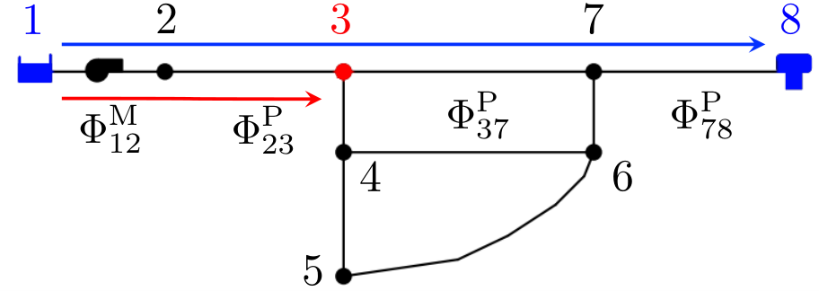
Notice that any head difference can be expressed as the linear combination of nonlinear models of pipes and pumps using $\bm{E}_{h}$. This key observation is thoroughly illustrated in Fig. 3(a) in Section IV. We note the following about the WDN-SE problem.

A geometric program [19] is a type of optimization problem can be expressed as

where $\bm{x}$ is an entry-wise positive optimization variable, $f_{i}(\bm{x})$ are posynomial functions and $g_{i}(\bm{x})$ are monomials.

One main requirement of the GP formulation is the positiveness of the decision variables, which limits some decision variables and physical constraints in our setting, e.g., flows in pipes and headloss equation. To overcome this modeling limitation we are inspired by linear programming (LP) techniques. In the simplex method[20], for example, the free variables are split into a positive and negative part, both being nonnegative. In our case, we introduce an exponential function $f(x)=b^{x}$ to convert a nonpositive variable to a positive one, since $f(x)$ is always positive. Using this technique, we can convert some problems with negative feasible regions into a new problem with a positive feasible region, and then solve it by using modern optimization solvers. This technique has been successfully applied to solve the control of WDNs in our recent work [16]. The SE problem here is similar to the control problem of WDNs; however, in the current paper, we convert the SE problem (12) into an LP or QP problem instead of a GP, which provides more elegant—and computationally more efficient—solutions.

Based on the newly introduced optimization technique in Section III-A, we first convert the nonlinear hydraulic model of WDNs into its GP form and then into its LP form. Here, we convert the head at the $i^{\mathrm{th}}$ node $h_{i}$ and the flow $q_{ij}$ into positive values ${\hat{h}_{i}}$ and ${\hat{q}_{ij}}$ through exponential functions, ${\hat{h}_{i}}\triangleq{b}^{h_{i}},\;{\hat{q}_{ij}}\triangleq{b}^{q_{ij}}$, where $b=1+\delta$ is a constant base and $\delta$ is a small positive number. Notice that we only need to convert the $\bm{\Phi}^{\mathrm{P}}(\bm{\cdot})$ and $\bm{\Phi}^{\mathrm{M}}(\bm{\cdot})$ into linear form because others are already linear. Tab. I show detailed conversions of all physical models that are all discussed in the following sections.

Next, we convert the pipe model, and let ${\hat{h}_{ij}^{\mathrm{P}}}$ be the GP form of head loss of a pipe, which is obtained by exponentiating both sides of (1) as follows

where $\widehat{C}_{ij}^{\mathrm{P}}(q_{ij})=b^{q_{ij}\left(R_{ij}{|q_{ij}|}^{\mu-1}-1\right)}$ is a function of $q_{ij}$. Hence, the head loss constraint for each pipe can be written as a monomial equality constraint, which is expressed as (3), if a an estimate of $\widehat{C}_{ij}^{\mathrm{P}}(q_{ij})$ is known. In order to make it linear, we can execute the $\log$ function on both sides of (3) and obtain (5) where $\widehat{C}_{ij}^{\mathrm{P}}(q_{ij})$ turns into $C_{ij}^{\mathrm{P}}(q_{ij})={q_{ij}(R_{ij}{|q_{ij}|}^{\mu-1}-1)}$.

We note that the expression above is linear with respect to $C_{ij}^{\mathrm{P}}(q_{ij})$ if ${q_{ij}}$ is known, hence we develop a method to find ${q_{ij}}$ by sequentially updating ${q_{ij}}$ and $C_{ij}^{\mathrm{P}}(q_{ij})$. The technique is introduced here. At first, we can make an initial guess denoted by $\langle{q_{ij}}\rangle_{0}$ for the $0^{\mathrm{th}}$ iteration ($\langle{C_{ij}^{\mathrm{P}}}\rangle_{0}$ can be obtained if $\langle{q_{ij}}\rangle_{0}$ is known), thus, for the $n^{\mathrm{th}}$ iteration, the corresponding values are denoted by $\langle{q_{ij}}\rangle_{n}$ and $\langle{C_{ij}^{\mathrm{P}}}\rangle_{n}$. If the flow rates are close to each other between two successive iterations, we can approximate $\langle{C_{ij}^{\mathrm{P}}}\rangle_{n}$ using $\langle{C_{ij}^{\mathrm{P}}}\rangle_{n-1}$, that is $\langle{C_{ij}^{\mathrm{P}}}\rangle_{n}\approx\langle{C_{ij}^{\mathrm{P}}}\rangle_{n-1}.$ Then, for each iteration $n$, we have

and it can be approximated by a constant given the flow value $\langle{q_{ij}}\rangle_{n-1}$ from the previous iteration.

Similarly, the new variables ${\hat{q}_{ij}}=b^{q_{ij}}$ and ${\hat{s}_{ij}}=b^{s_{ij}}$ for $(i,j)\in\mathcal{M}$ are introduced for pumps. Let ${\hat{h}_{ij}^{\mathrm{M}}}$ be the GP form of head increase of a pump

where $\widehat{C}_{1}^{\mathrm{M}}=b^{-{s_{ij}^{2}}h_{0}}$ and $\widehat{C}_{2}^{\mathrm{M}}=rq_{ij}^{\nu-1}s_{ij}^{2-\nu}$. Hence, the approximating equation for the pump head increase becomes the monomial equality constraint (4) in Tab. I. After executing $\log$ function on both sides of (4), the equation (6) can be obtained, which is a linear constraint. And at the same time, the parameters $\widehat{C}_{1}^{\mathrm{M}}$ and $\widehat{C}_{2}^{\mathrm{M}}$ become ${C}_{1}^{\mathrm{M}}$ and ${C}_{2}^{\mathrm{M}}$, that is

Parameters $C_{1}^{\mathrm{M}}$ are fixed, while $C_{2}^{\mathrm{M}}$ follow a similar iterative process as $C_{ij}^{\mathrm{P}}$. That is, starting with an initial guess for the flow rates and relative speeds, the constraints are approximated at every iteration via constraints abiding by the linear form, as listed in Tab. I. This process continues until a termination criterion is met. The details are further discussed in Algorithm 1.

After the conversion of pipe and pump model constraints, we can express the converted problem as

where constraints and variables remain the same as in (12) except that constraints (14c) and (14d) are now linear and viewed as constraints. The parameters $\bm{C}^{\mathrm{P}}$ is a $\mathbb{R}^{n_{p}\times 1}$ vector collecting the $C_{ij}^{\mathrm{P}}$ for each pipe. Similarly, the $\bm{C}_{1}^{\mathrm{M}}$ and $\bm{C}_{2}^{\mathrm{M}}$ are a $\mathbb{R}^{n_{m}\times n_{m}}$ diagonal matrices collecting $C_{1}^{\mathrm{M}}$ and $C_{2}^{\mathrm{M}}$ for each pump.

We note the following: (i) LP/QP-SE (14) is only an approximation of WDN-SE (12) at a specific point (the flow through pipes and pumps $q_{ij}$), in other words, the nonconvex WDN-SE can be approximated by successive convex LP/QP-SE. (ii) The converted model is linear but it is not the equivalent to the first order Taylor series linearization. We present the geometric meaning of the conversion we applied via a concrete example in Section IV-A1. (iii) LP/QP-SE can be expressed as either an LP or QP depending on the objective function. When $f(\bm{\epsilon})$ is modeled through the absolute weighted error, i.e., $\textstyle\sum_{k=1}^{T}\textstyle\sum_{i=1}^{n_{e}}w_{i}(k)|\epsilon_{i}(k)|$, the problem can be written as an LP. When it is based on WLS, then it becomes a standard QP.

In order to solve all the unknown variables, our algorithm needs to know the basic information at first, e.g., the topology of tested network to form the matrices $\bm{E}_{q}$, demand ${\bm{d}}$, measurements of head $\bm{\widetilde{}}{\bm{h}}$, and the accuracy matrix $\bm{W}$.

Notice that all variables are collected in $\bm{\xi}$ by (11) and the notation $\langle{{\bm{\xi}}}\rangle_{n}$ in Algorithm 1 stands for the $n^{\mathrm{th}}$ iteration value $\bm{{\xi}}$. For the $0^{\mathrm{th}}$ iteration, we initialize all flow $\langle{\bm{q}^{\mathrm{P}}}\rangle_{0}$ and $\langle{\bm{q}^{\mathrm{M}}}\rangle_{0}$ in $\langle{\bm{{\xi}}}\rangle_{0}$ with historical average flows. In fact, this algorithm still works by initializing all the flow in $\langle{\bm{{\xi}}}\rangle_{0}$ with random number. However, the convergence is relatively slow. All initial statuses of pumps, tanks, and reservoirs are initialized with the value set in “.inp” source file which is a standard input file used by EPANET, e.g., the initial status (open or close) and speed (if open) of pumps, and the initial head value $\langle{\bm{h}^{\mathrm{R}}}\rangle_{0}$ and $\langle{\bm{h}^{\mathrm{TK}}}\rangle_{0}$ of tanks and reservoirs. The parameters $\langle{C_{ij}^{\mathrm{P}}}\rangle_{1}$, $\langle{C_{1}^{\mathrm{M}}}\rangle_{1}$, and $\langle{C_{2}^{\mathrm{M}}}\rangle_{1}$ are then calculated by initialized values according to Section III-B, and all constraints are automatically generated for different WDNs topologies.

After solving (14) and obtaining the current solution $\langle{\bm{{\xi}}}\rangle_{n}$, and defining the iteration error as the Euclidean distance between two consecutive iterations, we set $\langle{\bm{{\xi}}}\rangle_{n}$ as the saved value for error calculation in next iteration by assigning ${{\bm{\xi}}_{\mathrm{save}}}=\langle{\bm{{\xi}}}\rangle_{n}$. The iteration continues until the error is less than a predefined threshold ($\mathrm{threshold}$) or a maximum number of iterations ($\mathrm{maxIter}$) is reached, and the final solution is ${{\bm{\xi}}_{\mathrm{SE}}}$.

The bottleneck of this algorithm is solving a scalable LP/QP successively which should not cause a large computational burden, even if tens of iterations are required to converge. We note that Steps 7 and 8 are used to accelerate the computational times, since the direction of the search is known, and the acceleration parameter $a$ in Step 8 is needed to be adjusted according to the specific WDN. This will be investigated in future work. We finally note that Algorithm 1 does not show the windowing process of performing real-time SE, as the algorithm only shows batch state estimation. However, a moving horizon window can be implemented within Algorithm 1 thereby allowing real-time state estimation.

The 3-node network comprised of 3 junctions and 2 pipes is shown in Fig. 1(a), and no demand at Junctions 2 and 4.

The 8-node network from EPANET Users Manual [18] is a looped network, and labels for various components are all shown in Fig. 3(a). If the head at reservoir and tank, $h_{1}^{\mathrm{R}}$ and $h_{8}^{\mathrm{TK}}$, are known, then it satisfies the sufficient scenario which means the solution can be determined with just these two measurements. The solution $\bm{\xi}_{\mathrm{SE}}$ solved by Algorithm 1 and $\bm{\xi}_{\mathrm{EPANET}}$ from EPANET are given in Tab. IV(b) when $h_{8}^{\mathrm{TK}}=834\ \mathrm{ft}$ and $h_{1}^{\mathrm{R}}=700\ \mathrm{ft}$, and final error $\lVert\bm{\xi}_{\mathrm{SE}}-\bm{\xi}_{\mathrm{EPANET}}\rVert$ presented in Fig. 3(b) reaches 0.1 which illustrates the effectiveness of proposed method.

As we mentioned in Section II-B, we assume that the measurements of heads at tanks and reservoirs are very accurate. We measure one more head at Junction 3 ($h_{3}$) thereby defining the over-determined scenario. There are two cases based on which measurement is more trustful. For Case 1, if we postulate that $h_{8}^{\mathrm{TK}}=834.60\ \mathrm{ft}$ is more accurate and setting the accuracy matrix as $W=\diag(1,0.1)$, we see the resulting $h_{8}^{\mathrm{TK}}$ is very close to the measured value in Tab. IV(b), while $h_{3}$ is far from its measurement since it is considered less accurate. For Case 2, if $h_{3}$ is considered more accurate, $h_{3}$ is close to its measured value $875.64\ \mathrm{ft}$. Besides that, the two estimated variables $h_{5}$ and $q_{46}$ are shown, and we can see that both are close to the values provided by the EPANET software, but vary slightly between Cases 1 and 2.

References

- [1] W. Zhao, T. H. Beach, and Y. Rezgui, “Optimization of potable water distribution and wastewater collection networks: A systematic review and future research directions.” IEEE Trans. Systems, Man, and Cybernetics: Systems, vol. 46, no. 5, pp. 659–681, 2016.
- [2] V. Puig, C. Ocampo-Martinez, R. Pérez, G. Cembrano, J. Quevedo, and T. Escobet, Real-Time Monitoring and Operational Control of Drinking-Water Systems. Springer, 2017.
- [3] K. S. Tshehla, Y. Hamam, and A. M. Abu-Mahfouz, “State estimation in water distribution network: A review,” in Industrial Informatics (INDIN), 2017 IEEE 15th International Conference on. IEEE, 2017, pp. 1247–1252.
- [4] A. Aisopou, I. Stoianov, and N. J. Graham, “In-pipe water quality monitoring in water supply systems under steady and unsteady state flow conditions: A quantitative assessment,” Water research, vol. 46, no. 1, pp. 235–246, 2012.
- [5] W. Cheng, T. Yu, and G. Xu, “Real-time model of a large-scale water distribution system,” Procedia Engineering, vol. 89, pp. 457–466, 2014.
- [6] S. Vrachimis, D. Eliades, and M. Polycarpou, “Real-time hydraulic interval state estimation for water transport networks: A case study,” Drinking Water Engineering and Science, vol. 11, pp. 19–24, 03 2018.
- [7] A. Bargiela, “On-line monitoring of water distribution networks,” Ph.D. dissertation, Durham University, 1984.
- [8] R. Powell, “State estimation in water networks: a tutorial,” Measurement and control, vol. 32, no. 4, pp. 101–104, 1999.
- [9] J. Davidson and F.-C. Bouchart, “Adjusting nodal demands in SCADA constrained real-time water distribution network models,” Journal of Hydraulic Engineering, vol. 132, no. 1, pp. 102–110, 2006.
- [10] B. D. Barkdoll and H. Didigam, “Effect of user demand on water quality and hydraulics of distribution systems,” in World Water & Environmental Resources Congress 2003, 2003, pp. 1–10.
- [11] M. Pasha and K. Lansey, “Analysis of uncertainty on water distribution hydraulics and water quality,” in Impacts of Global Climate Change, 2005, pp. 1–12.
- [12] D. Kang, M. Pasha, and K. Lansey, “Approximate methods for uncertainty analysis of water distribution systems,” Urban Water Journal, vol. 6, no. 3, pp. 233–249, 2009.
- [13] F. Fusco and E. Arandia, “State estimation for water distribution networks in the presence of control devices with switching behavior,” Procedia Engineering, vol. 186, pp. 592–600, 2017.
- [14] A. Preis, A. J. Whittle, A. Ostfeld, and L. Perelman, “Efficient hydraulic state estimation technique using reduced models of urban water networks,” Journal of Water Resources Planning and Management, vol. 137, no. 4, pp. 343–351, 2011.
- [15] R. Duffin, E. Peterson, and C. Zener, Geometric programming - theory and application. New York: Wiley, 1967.
- [16] S. Wang, A. F. Taha, N. Gatsis, and M. Giacomoni, “Geometric programming-based control for nonlinear, dae-constrained water distribution networks,” in 2019 American Control Conference, Philadelphia, US, July 2019, pp. 1470–1475. https://arxiv.org/pdf/1902.06026.pdf
- [17] A. S. Zamzam, E. Dall’Anese, C. Zhao, J. A. Taylor, and N. Sidiropoulos, “Optimal water-power flow problem: Formulation and distributed optimal solution,” IEEE Transactions on Control of Network Systems, 2018.
- [18] L. A. Rossman et al., “Epanet 2: users manual,” 2000.
- [19] S. Boyd, S.-J. Kim, L. Vandenberghe, and A. Hassibi, “A tutorial on geometric programming,” Optimization and engineering, vol. 8, no. 1, p. 67, 2007.
- [20] I. J. Lustig, R. E. Marsten, and D. F. Shanno, “Interior point methods for linear programming: Computational state of the art,” ORSA Journal on Computing, vol. 6, no. 1, pp. 1–14, 1994.
- [21] D. Elíades and M. Kyriakou, “Epanet matlab toolkit,” University of Cyprus, Republic of Cyprus, 2009.
- [22] I. CVX Research, “CVX: Matlab software for disciplined convex programming, version 2.0,” http://cvxr.com/cvx, Aug. 2012.
- [23] “Shenwang9202/state estimation,” accessed 15 March 2019. https://github.com/ShenWang9202/StateEstimation