Receding Horizon Control for Drinking Water Networks: The Case for Geometric Programming
Abstract
Optimal, network-driven control of WDN (WDN) is very difficult: valve and pump models form non-trivial, combinatorial logic; hydraulic models are nonconvex; water demand patterns are uncertain; and WDN are naturally large-scale. Prior research on control of WDN addressed major research challenges, yet either (i) adopted simplified hydraulic models, WDN topologies, and rudimentary valve/pump modeling or (ii) used mixed-integer, nonconvex optimization to solve WDN control problems.
The objective of this paper is to develop tractable computational algorithms to manage WDN operation, while considering arbitrary topology, flow direction, an abundance of valve types, control objectives, hydraulic models, and operational constraints—all while only using convex, continuous optimization. Specifically, we propose new GP (GP)-based MPC (MPC) algorithms, designed to solve the water flow equations and obtain WDN controls, i.e., pump/valve schedules alongside heads and flows. The proposed approach amounts to solving a series of convex optimization problems that graciously scale to large networks. The proposed approach is tested using a 126-node network with many valves and pumps and shown to outperform traditional, rule-based control. The developed GP-based MPC algorithms, as well as the numerical test results are all included on Github.
Index Terms:
Water distribution networks, geometric programming, model predictive control, pump and valve control.List of Acronyms
- CDF
- Cumulative Distribution Function
- DAE
- Difference Algebraic Equation
- DSE
- Deterministic State Estimation
- EPS
- Extended Period Simulation
- FCV
- Flow Control Valve
- FOSM
- First-Order Second-Moment
- GP
- Geometric Programming
- GPV
- General Purpose Valve
- HVC
- Half Vectorization Covariance
- ISE
- Interval State Estimation
- LAV
- Least Absolute Value
- LP
- Linear Programming
- LS
- Least Square
- MCS
- Monte Carlo Simulation
- MPC
- Model Predictive Control
- Probability Distribution Function
- PRV
- Pressure Reducing Valve
- PSE
- Probabilistic State Estimation
- RBC
- Rule-based Control
- SBSE
- Set Bounded State Estimation
- SCADA
- Supervisory Control and Data Acquisition
- SE
- State Estimation
- WDN
- Water Distribution Networks
- WFP
- Water Flow Problem
- WLAV
- Weighted Least Absolute Value
- WLS
- Weighted Least Square
I Introduction and Paper Contributions
Water distribution networks (WDN) are large-scale critical infrastructures. The real-time management and operation of WDN considering economic and environmental factors have gained an increasing interest from various engineering and social science disciplines. With the expansion of cities, the complexity of WDN poses challenges for water utilities taking into account multiple—potentially conflicting—objectives such as minimizing economic costs, guaranteeing the stability and security of the network, and maintaining safe water levels in tanks.
The very basic decision-making problem involved in WDN operation, the WFP (WFP), is to solve for the water flow and head (i.e., the energy) given water demand forecasts. The hydraulic models of head loss and water flow across pipes, valves, and pumps are nonlinear—especially when considering different kinds of valves and pumps. This subsequently makes it very difficult to find optimal management/operation strategies incorporating the WFP in a computationally efficient way. In short, the basic WFP constraints (nonconvex constraints modeling hydraulics of heads and flows) show up in an abundance of WDN problem formulations. These formulations include the hour-ahead operation of pumps and valves, pipe burst detection, water quality control, and sensor placement in water networks, to name a few [1].
I-A Literature review
The literature on solving the nonconvex WFP as well as other related problem formulations is rich and briefly summarized next. The main classical approaches to solve the WFP are based on Hardy-Cross [13], Newton-Raphson [14, 15, 16], linearization [17, 18], optimization [19, 20], gradient-based [21], and more recently, fixed-point methods [22, 23]. All of these methods are iterative algorithms developed to solve a set of linear and nonlinear equations to obtain the physical status of WDN, i.e., the flow through each link or the head at each node. These methods differ in terms of convergence speed and limitations. The authors in [24] produce a thorough discussion on the uniqueness of the WFP solution for various types of networks.
Several methods have been developed to solve the operation, scheduling, and planning problems incorporating the WFP and have been recently surveyed in [1] in great detail. One of these methods is based on model predictive control (MPC), also known as receding horizon control, with formulations reported in [25, 2, 3, 4, 5]. These are reviewed next, as they relate to the scope of this paper. Specifically, the authors in [25] present a stochastic MPC formulation to handle uncertainty in WDN and apply the proposed MPC to the Barcelona drinking water network with real demands. The study [2] obtains optimal management strategies in urban water cycle via MPC. The authors in [3] address a nonlinear economic MPC strategy to minimize the economic costs associated with pumping and water treatment. A nonlinear MPC controller is designed in [4] to meet consumer demands at desired pressures. The authors in [5] consider a robust controller to maintain stable operation of water flow rate, and to reduce the operational cost by manipulating the pump speed via MPC.
As for the optimal control of WDN, there are various factors listed in Tab. I needed to be considered from an engineering standpoint. For example, some research methods only consider simplified WDN topology, the rather simpler, quadratic head loss model, fixed-speed pumps, and simple valve models which can be viewed as constraints with upper and lower bounds on the flow. Besides that, the pump cost model is assumed as fixed or quadratic in many studies, and other methods fail to consider the influence of dynamic electricity prices or pump efficiency. All studies and corresponding considerations related to optimal control in WDN are presented and compared in Tab. I.
When combining the WFP with the dynamics of water tanks and operation of pumps and valves, a set of nonlinear difference algebraic equations (DAEs) can be formulated to model WDN. Some of the recent methods to deal with the nonlinear DAEs are (a) linearizing the WFP constraints and corresponding objective functions [2, 25, 26, 27, 28], (b) constructing relaxations for the nonlinear relationships to derive lower bounding linear programs [29, 30, 6], (c) keeping the nonlinearities and formulating the problem as a nonconvex program [31, 32, 3, 7], and (d) applying convex approximations/relaxations to convert the nonconvex problem into a convex one [33, 8, 9, 34, 35, 6, 36].
The studies closest to our paper are [8, 33, 9, 7, 6]. The authors in [6] perform pump scheduling with a (non)linear programming based branch and bound method, and a tight mixed integer linear relaxation of the original non-convex formulation is devised and solved. In [7], the authors use a mixed-integer nonlinear program (MINLP) model incorporating both the nonlinear physical laws and discrete decisions, and algorithmic techniques such as branch-and-bound and linear approximation are applied to solve the MINLP to -global optimality. In [33], the authors use GP approximations and convert the nonconvex head loss equations into GP form, and hence a globally optimal solution is guaranteed. An important contribution of [33] is that the proposed GP method is non-iterative (i.e., it is a one-shot optimization problem). However, this approach operates under the assumption that the network has a tree topology or that flow directions are known. Studies making similar assumptions include [8, 37]. The authors in [9] model the optimal scheduling of WDN as a mixed-integer second-order cone program, which is analytically shown to yield WDN-feasible minimizers under certain sufficient conditions.
| Original hydraulic model | DAEs | GP form | Abstract GP | |
| Tanks | (1) | (18a) | (2) | (31a) |
| Junction nodes | (3) | (18b) | (4) | (31b) |
| Pipes | (5) | (6) | (31c) | |
| Pumps | (7) | (8) | (31d) | |
| Valves (GPV) | (9) | (18c) | (10) | (31e) |
| Valves (PRV) | (11) | (12) | (31e) (25) | |
| Valves (FCV) | (13) | (14) | (31e) (25) | |
| Constraints | (15a) (15b) (15c) (15d) (15e) (15f) | (19) | (16a) (16b) (16c) (16d) (16e) (16f) | (25) |
I-B Paper contributions
The objective of this paper is to develop tractable computational algorithms based on convex programming to manage WDN operation through an MPC scheme. Specifically, this paper presents an MPC algorithm considering arbitrary network topology, tank volume dynamics, realistic pump cost models, arbitrary flow directions, and an abundance of valve types, control objectives, and operational constraints. The main contributions of this paper are summarized as follows.
- •
We derive a nonlinear DAE model of WDN that incorporates discrete-time tank dynamics, models depicting conservation of mass and energy, any of the three common empirical head loss equations (Hazen-Williams, Darcy-Weisbach, and Chezy-Manning), various types of valves [ GPV (GPV), PRV (PRV), and FCV (FCV)] as well as general models of pumps (variable or fixed speed pumps). Given the general nonlinear DAE model, we formulate a nonlinear MPC that includes the DAE-constrained model, three important objective functions for WDN management (water safety level, smoothness of control action, and pump costs), and other operational constraints on pumps, valves, and tanks. Sections II and III present this contribution.
- •
To deal with the non-convexity of the MPC formulation, geometric programming (GP) methods are investigated to furnish WDN controllers managing pumps and valves without restricting the WDN graph topology and most importantly, without assuming knowledge of the water flow direction. The proposed approach amounts to solving a series of convex GP problems, and is embedded within the MPC, resulting in a computationally tractable problem.** * Solvers using standard interior-point algorithms can solve a GP with 1,000 variables and 10,000 constraints in under a minute on a small computer. For sparse problems, a typical GP with 10,000 variables and 1 million constraints can be solved in minutes on a desktop computer [38]. The approximation of the nonconvex problem by a convex one is presented in Section IV.
- •
To assess the applicability of the proposed methods, the Battle of the Water Sensor Networks (BWSN) 126-node water network [39, 40] with multiple valves and pumps is utilized. Specifically, the case study illustrates how the formulated algorithms have the potential to manage WDN in real-time while incorporating uncertainty in the water demand patterns. The algorithms are implemented within EPANET [41] and provided in Section VI. To make this work accessible to interested readers and practitioners, we also include a link [42] to the codes used to generate the abstract DAE model, the GP transformation, and the proposed algorithms in addition to the results obtained in the case studies section of this paper. The codes allow the user to input a different WDN benchmark. A preliminary version of this work appeared in [43] where we considered only the pump control problem without incorporating various types of valves or a realistic pump cost curve. The present paper thoroughly extends the methods in [43].
II Control-Oriented Modeling of WDN
We model WDN by a directed graph . Set defines the nodes and is partitioned as where , , and respectively stand for the collection of junctions, tanks, and reservoirs. Let be the set of links, and define the partition , where , , and respectively stand for the collection of pipes, pumps, and valves. For the node, set collects its neighboring nodes and is partitioned as , where and stand for the collection of inflow and outflow nodes. It is worth emphasizing that the assignment of direction to each link (and the resulting inflow/outflow node classification) is arbitrary, as the presented optimization problems yield the direction of flow in each pipe. Tab. III summarizes the set and variable notations in this paper. The WDN are comprised of active and passive components. The active components can be controlled for management purpose and include pumps and valves, while the passive components comprising junctions, tanks, reservoirs, and pipes cannot be controlled.
The basic hydraulic equations describing the flow in WDN are derived from the principles of conservation of mass and energy. In WDN, the former implies that the rate of change in the water storage volume is equal to the difference between the system inflow and outflow and the latter states that the energy difference stored in a component is equal to the energy increases minus energy losses, such as frictional and minor losses [44]. According to these basic laws, the equations that model mass and energy conservation for all components (passive and active) in WDN can be written in explicit and compact matrix-vector forms in the first three columns of Tab. II. The last two columns of Tab. II are needed in the ensuing sections of the paper. The various component models are reviewed next.
II-A Models of passive components
II-A1 Tanks and Reservoirs
II-A2 Junctions and Pipes
Junctions are the points where water flow merges or splits. The expression of mass conservation of the junction at time can be written as (3) in Tab. II, and stands for end-user demand that is extracted from node . The real demand is almost impossible to know in advance, hence the predicted or estimated one is used in our paper, and the introduced uncertainty is handled via MPC.
The major head loss of a pipe from node to is due to friction and is determined by (5) from Tab. II, where is the resistance coefficient and is the constant flow exponent in the Hazen-Williams, Darcy-Weisbach, or Chezy-Manning formula [45]. The approach presented in this paper considers any of the three formulae [45, 41]. Minor head losses are ignored in this paper, although the presented algorithms still apply seamlessly when minor head losses are considered
| Notation | Set Notation Description |
| A set of nodes including junctions, tanks and reservoirs | |
| A set of links including pipes, pumps and valves | |
| A set of junctions | |
| A set of tanks | |
| A set of reservoirs | |
| A set of pipes | |
| A pair set of pumps | |
| A pair set of valves | |
| A set of neighbors node of the node, | |
| A set of inflow neighbors of the node, | |
| A set of outflow neighbors of the node, | |
| Variable Notation Description | |
| Head at node | |
| Head at tank | |
| Head at reservoir | |
| Head loss for the pipe from to | |
| Head loss/increase for the pump from to | |
| Head loss for the valve from to | |
| Flow through a pipe, valve or pump from node to node | |
| The flow value at time | |
| the iteration value of |
II-B Models of active components
II-B1 Head Gain in Pumps
A head increase/gain can be generated by a pump between the suction node and the delivery node . The pump properties decide the relationship function between the pump flow and head increase [45], [41, Chapter 3]. Generally, the head gain can be expressed as (7), where is the shutoff head for the pump; is the flow through a pump; is the relative speed of the same pump; and are the pump curve coefficients. It is worthwhile to note that (a) the in (7) is always nonpositive, and this can be viewed as an operational constraint (15f), (b) this head gain model of a pump cannot describe the condition of the pump being off which potentially reduces the pump cost, and we define it as incompleteness of head gain model. When a pump is off, speed and flow are equal to zero; and no constraint exists between and , which indicates that they are decoupled. This entails that constraint (7) is removed from the WDN model.
II-B2 Valves
Several types of valves can be controlled in WDN, and they can be expressed as a component between junctions and . Typically, the control valves are GPVs, PRVs, and FCVs and the corresponding variables are valve openness, pressure reduction, and flow regulation. The valve models in our paper are based on EPANET Users’ Manual; see [41, Chapter 3] for more details. We next discuss the types of valves considered in this work.
GPVs are used to represent a link with a special flow-head loss relationship instead of one of the standard hydraulic formulas. They can be used to model turbines, well draw-down or reduced-flow backflow prevention valves [41, Chapter 3.1]. In this paper, we assume that the GPVs are modeled as a pipe with controlled resistance coefficient and can be expressed as (9) in Tab. II, where is a control variable depicting the openness of a valve assuming GPVs can be fully open but never closed, and the other variables are the same as in the pipe model. Similar to the incompleteness of head gain model of the pump, turning a GPV off is not equivalent to setting the openness of the valve to . When a GPV is off, no constraint exists between and , which indicates that they should be decoupled. However, if the openness is set to , it results in the erroneous . Hence, constraint (9) cannot describe the closedness of a GPV, and therefore we assume that GPVs cannot be completely off.
PRVs limit the pressure at a junction in the network (reverse flow is not allowed) and set the pressure on its downstream side when the upstream pressure is higher than [41, Chapter 3.1]. Assuming that the upstream side is denoted as , and the downstream side is , the PRVs can be modeled by (11) in Tab. II where is the pressure setting converted to head via where is the elevation at junction and parameter is the pressure setting of the PRV and both are constants. Therefore, the head is fixed.
We use the same logic in [41, Appendix D] to change the status of a PRV, and only one case is presented here:
| (17) | ||||
The logic above could be viewed as a conditional form constraint, and the resulting combinatorial relationship requires modeling using integer variables. To avoid using MINLP, this conditional logic is mimicked through successive iterations. Our motivation here is to maintain a tractable, convex programming formulation through approximations and heuristics that capture some depth in regards to the complex modeling of WDN components.
We denote as the iteration value of , hence, stands for at the , , , iteration. From the above logic, we can see the current status of a PRV is decided by the previous status and the or . Supposing that the iteration is the , and thus that and can be solved for based on the known status, e.g. ACTIVE, then the current status of PRV can be determined according to the solved flow or head. Thus, if the status is determined to be OPEN or ACTIVE, the corresponding constraint from (11) is applied in the next iteration; if it is detemined to be CLOSED, then and are decoupled. To sum up, the conditions in if statement are checked in the previous iteration and the conclusion in the then statement is applied to the current iteration. This technique is applied repeatedly in the ensuing sections.
FCVs limit the flow to a specified amount when , and are treated as the open pipes when , that is, when the flow is reversed, implying that the valve cannot deliver the flow. The functionality of FCVs can thus be modeled by (13), where is the setting value. The logic to update the status of a FCV can be described by
We apply the same technique for the conditional logic, and for more details of the logic to change the status of a FCV, please refer to [41, Appendix D]. The corresponding DAE model of WDN is presented next.
| Symbol | Description | Dimension |
| A vector collecting heads at tanks | ||
| A vector collecting heads at junctions | ||
| A vector collecting heads across pumps | ||
| A vector collecting flows through controllable elements, e.g., pumps and valves | ||
| A vector collecting flows through pumps | ||
| A vector collecting flows through valves | ||
| A vector collecting flows through uncontrollable elements, e.g., pipes | ||
| A vector collecting the relative speed of pumps | ||
| A vector collecting the openness of GPVs | ||
| A vector collecting demands at junctions | ||
| A vector collecting , , , , , at time | ||
| The GP form of vector |
II-C Difference algebraic equations form of WDN model
The WDN model in the previous section can be abstracted to DAEs as (18). Define , , , , , and to be vectors of appropriate dimensions listed in Tab. IV. Collecting the mass and energy balance equations of tanks (1), junctions (3), pipes (5), pumps (7) and valves (9), (11), and (13), we obtain the following DAE model
| (18a) | ||||
| (18b) | ||||
| (18c) | ||||
where , , and are constant matrices that depend on the WDN topology and the aforementioned hydraulics and is a zero-vector of size . The function collects the nonlinear components in (5), (7), (9), (11), and (13). The state-space matrices above can be generated by our Github code [42] for any WDN.
III MPC-based Problem Formulation
This section derives an MPC-based formulation given the derived nonlinear DAE model (18). The constraints, objective functions, and overall problem formulation are given next. The physical constraints pertaining to (18) can be written as Constraints:
| (19) |
The above constraints model upper and lower bounds on the heads of junctions, tanks and reservoirs, pump speeds, and flows are expressed as equations (15a)–(15f) in Tab. II. We also assume that the relative speed of all pumps can be modulated in the interval . Multiple objectives can be applied depending on operational considerations. In this paper, we consider three objectives expressed through
| (20a) | ||||
| (20b) | ||||
| (20c) | ||||
where enforces maintaining the safety water storage decided by the operator; is a vector collecting the safety head levels of tanks; enforces the smoothness of control actions through which stands for the flow rate changes of controllable components from time to ; and enforces minimization of the pump cost at time determined by
| (21) |
where denotes the water density; is the standard gravity coefficient; is the efficiency of pump across node and and is a function of flow ; and are the head increase and flow provided by the pump; in is the price of electricity. Considering a fixed , then represents the energy cost of a pump as depicted in Fig. 1 for a hypothetical example. We note that is nonlinear and nonconvex; is also a function of speed as well after substituting (7) into (21), and we can see that maintaining a low pump speed can effectively reduce pump costs [46]. We define and let vector collect , and we also define vectors and collecting and ; notice that and can be written in terms of and . Hence, is written in matrix form according to (20c), where operator stands for the element-wise product of two matrices.

We define a vector collecting all the optimization variables from to as follows
where is the prediction horizon of the MPC. Note that the indexing for is different in due to the fact that the initial conditions of the tanks are known, unlike other optimization variables such as the flow and the pump controls which we need to solve for from through . The weighted, multi-objective cost function can be written as
where is the corresponding weight for . Similar objective functions have been used before in [2, 27].
It is worth noticing that conflicts exist among the objectives. For example, the safe water level objective tends to speed the pump up to maintain the head in tanks, while minimizing the pump cost objective tries to bring the cost to by slowing pumps down and even turning pumps off.
Here, we propose using MPC to solve the WDN operation problem considering the nonlinearities and nonconvexities presented in the energy balance equations in WDN-DAE. The motivation for using MPC here is two-fold. First, the surge in adopting wireless sensing technologies and water meters in WDN enables near real-time monitoring which can be used to measure the WDN’s state. That is needed and useful for any MPC routine. Second, MPC is known to handle uncertainty in dynamic systems—a key quality that we exploit here. The MPC can be written as
| (22) |
Problem (22) is nonlinear and nonconvex due to the head loss models of pipes and pumps. WDN-MPC solves for flows, heads, the pump and valve controls while requiring a prediction of the nodal water demand for a horizon of length and initial tank levels . Since the nonconvexity in the head loss models takes an exponent shape, GP presents itself as a great alternative to solve the nonconvex problem.
Motivated by the literature gaps discussed in Section I, we propose a new GP-based MPC routine which is convex in the variables, considers various kinds of valves and pumps, while not requiring prior knowledge of water flow direction or a tree network topology.
IV GP Modeling of WDN
A basic introduction to GP is given in Appendix A with some needed definitions and properties. First, we introduce the conversion of the nonconvex hydraulic models in WDN-MPC (22) to their corresponding convex, GP form.
IV-A Conversion of variables
Here, we propose a GP model by mapping the optimization variable in (22) into its exponential form. The conversion helps to map all of the non-positive values into positive ones. Specifically, we convert the head and demand at the node and , the flow , relative speed , and openness of valve into positive values , , , , and through exponential functions, as follows
| (23) |
where is a constant base and is a small positive number. The variables , , , , and are positive which can then be used to transform the nonconvex WDN-MPC (22) into a GP. Converting the junction and tank physical models as well as constraints—all linear in the variables—follows from the above exponential mapping (23), while converting the pipe, pump and valve models into GP form is more complicated. The last two columns of Tab. II show detailed and abstract versions of the conversions of all physical models. The details of these conversions are discussed in the following sections.
IV-B Conversion of mass and energy balance equations
For the models of tanks and junctions, the conversion process is straightforward. After exponentiating both sides of (1) and (3), variables , , and are changed into , , and , while constraints (1) and (3) are converted to monomial equality constraints (2) and (4) in Tab. II.
In order to clearly show the derivation for pipes, the index is ignored at first. At time , let be the GP form of head loss of a pipe, which is obtained by exponentiating both sides of (5) as follows
where is a function of .
Note the following: (a) The flow is unknown at each time and the premise is to solve a series of convex optimization problems to find the final value for each time . (b) Instead of , the optimization variable is , thus is unknown but not a variable. The key challenge is that and are unknown but not variables, thereby motivating the need to develop a method to find the . The technique we mentioned in Section II-B is applied here. At first, we can make an initial guess denoted by for the iteration ( can be obtained if is known), thus, for the iteration, the corresponding values are denoted by and . If the flow rates are close to each other between two successive iterations, we can approximate using , that is Then, for each iteration at time ,
can be approximated by a constant given the flow value from the previous iteration. With this approximation, the head loss constraint for each pipe can be written as a monomial equality constraint
which is expressed as (6).
Similarly, the new variables and for are introduced for pumps. Let be the GP form of head difference of a pump:
where and . Parameters and follow a similar iterative process as . That is, they are treated at the iteration as constants based on the flow and relative speed values at the iteration. Hence, the approximating equation for the pump head increase becomes the monomial equality constraint (8), where is a constant parameter determined by the pump curve.
As for valves, the derivation of GPVs is the same as pipes except an extra variable for is introduced. At time , let be the GP form of head loss of a valve, which is obtained by exponentiating both sides of (9) as follows
where is a similar parameter as the parameters in pipe and pump models. For PRVs and FCVs, the conversion process is straightforward and equations (12) and (14) can be obtained after exponentiating both sides of (11) and (13).
Therefore, starting with an initial guess for the flow rates and relative speeds, the constraints are approximated at every iteration via constraints abiding by the GP form, as listed in Tab. II. This process continues until a termination criterion is met. The details are further discussed in Algorithm 2, after the presentation of the abstract GP form and the conversion of the control objectives in the next section.
IV-C Abstract GP model
IV-D Conversion of control objectives and GP-MPC formulation
In this section, we convert the control objectives in the nonconvex WDN-MPC to their convex, GP-based form.
IV-D1 Conversion of
In (20a), notice that is a vector collecting the head at tanks. The objective encourages to be close to the constant . Hence, we introduce a new auxiliary variable which is pushed to be close to . Using the epigraph form, the original objective function is replaced by and constraints are added as follows
Safety-GP:
| (26a) | ||||
| (26b) | ||||
where and are the GP form of and . If the water level of the tank is below the safe level, the corresponding constraints are and . These constraints force close to , but it is possible that the safe water level can never be reached if the flow is limited in a certain period of time or the safe water level is set to an unreasonable high value. Otherwise, variable is set to , which implies no objective function is applied at the tank. Notice that constraint (26) is in conditional form, and the technique we mentioned in Section II-B is applied again. Hence, the condition is checked at the end of the previous iteration and the corresponding constraints in (26) are applied at the current iteration.
IV-D2 Conversion of
Moving to the second part of the objective function (20b), is a vector collecting the flow changes of controllable flow between and (). We introduce a new auxiliary variable and perform an element-wise exponential operation on both sides of (20b) yielding
where , and and are variables. Similar to the situation converting the pipe model in Section IV-B, is not a variable since it is estimated from previous iteration. The current iteration can be set to the previous one that is known. Using the epigraph form, the original objective function can be expressed as a new objective and constraints are given as Smoothness-GP:
| (27a) | ||||
| (27b) | ||||
where parameter stands for the extent of smoothness: the smaller it is, the more smooth the control actions can be. Note that is our desired smoothness, and it is possible that cannot reach it. In other words, if reaches , then this means there is more room to adjust the flows of controllable elements, and could be set smaller if desired.
IV-D3 Conversion of
The incompleteness of head gain model introduced in Section II-B wipes the possibility to find the optimal cost as the pump has to be always on and cannot be off. Two possible methods to handle this issue are the following: (a) introducing an integer variable, making it stand for the on-off status of a pump, and forming the overall problem as an MINLP; or (b) instead of using the cost of pumps as an objective function, we develop a heuristic algorithm which turns part or all of the pumps off and calculates the total cost of pumps by (20c) after each iteration.
Given the above derivations, the final GP form of multi-objective cost function can be rewritten as
| (28) |
where is a posynomial function and is a weight reflecting the preference of the WDN operator.
The convex GP-based MPC can now be expressed as
| (29) | |||||
In (29), two sets of optimization variables are included. The first set comprises , , , , , and which are collected in variable . The second set includes the auxiliary variables and introduced before. Notice that the flow is an optimization variable while is not in GP-MPC, but a value used to calculate , , , and . The detailed GP constraints are given in Tab. II.
GP-MPC is convex, and similar to MPC-WDN both can be infeasible when some parameters are physically unreasonable, e.g., the demand is too high or the pumps are not powerful enough to provide enough flow for all nodes in the network. The next section proposes a real-time algorithm to manage WDN and control pumps and valves.
V Real-Time Management of WDN
The control architecture is presented in Fig. 2. First, we compute the state-space DAE matrices, build the GP model of WDN and solve the GP-MPC after analyzing the source file (.inp is the input file for EPANET software). After obtaining the solution at , the control action is applied to the WDN via EPANET. The WDN state as well as more accurate demand signals are then obtained. The routine details are also given in Algorithm 1 which calls Algorithm 2. Algorithm 1 is tailored to the case where each pump is associated with a tank and vice versa, which is a typical arrangement in water distribution networks; we denote the association as pump-tank pair meaning .
The flow through pipes, valves, and pumps and the head at nodes in WDN can be solved when water demand forecasts, the statuses of pumps and valves, and the water level in tanks are given. However, the valve and pump control problems are challenging as the statuses of pumps and valves are variables. To address this, we consider the following: (a) PRVs and FCVs can adjust their status automatically if their previous statuses and current head and flow are given as we mentioned in Section II-A. Our algorithm calculates snapshots of hydraulic states in WDN at each iteration, and then the statues of all the controlled PRVs and FCVs are updated according to the solved solution. As for GPVs, we assume that GPVs are always on (although openness variable can be very close to zero), and the openness of a GPV can be obtained by Algorithm 2. (b) The statuses of pumps are determined by the binary search part in Algorithm 2.
Algorithm 2 is developed to search for smaller operational cost by turning pumps on/off for a single optimization window. The search steps are similar to the general binary search algorithm [47] and the search window is defined as , which is initialized as and . We define as the maximum number of time slots within the search window where any given pump is switched off. The initial is set to indicating no pump is switched off at first, and the solution and cost can be solved and saved. The variable records the number of tanks that reach unsafe water levels across time periods in the window and is saved as when . If the number increases () when , indicating that more safe water levels fail due to more pumps being switched off, we denote this situation by setting and the window is updated by , otherwise, it is updated as . Detailed examples are given in Section VI.
After the number of time periods is determined by the binary search, the key is to determine in which time periods the pumps should be switched off so that the objectives can be reached while minimizing costs. A simple strategy is turning off the pumps in the top expensive time slots according to the electricity price , and the time slot should be excluded if the safe water level is still unreached or .
During all prediction horizons, the on-off statuses of pumps are viewd as known (a pump is off in slots and on in slots). The next step is to find the solution when is fixed. As the technique we mentioned in Section II-B is applied here again, the notation stands for the iteration value of at time . We use the same notation system during iterations, e.g., is the iterate value of . We initialize the flow and in with historical average flows in the pipes and pumps, and both and are set to . The parameters , ,, and are then calculated according to Section IV-B, and all of the constraints and objectives can be automatically generated for different WDN.
After solving (29) and obtaining the current solution and the iteration error, we set as the initial value for next iteration by assigning . In addition, we define the error as the distance between current solution and previous solution . The iteration continues until the error is less than a predefined error threshold () or a maximum number of iterations () is reached. During iterations, the total pump cost of each iteration is also saved. This heuristic is faithful to the intricacies of WDN constraints and pump/valve modeling, does not use integer variables, and its main effort amounts to solving scalable GPs.
It is worth emphasizing that a solution produced from the successive iterations enclosed between lines 4 through 35 in Algorithm 2 is guaranteed to be feasible for problem (22), as long as the while loop in line 4 is exited due to the condition that the distance between two successive iterates is below a threshold. The feasibility follows from the construction of the monomial equality constraints in Section IV-B. In the vast majority of our numerical experiments, and for an array of different initializations of the algorithm, the condition on the proximity of two successive iterates was indeed satisfied, yielding no issues with the feasibility of the proposed control schedule for the WDN.
VI Case Study 1: The BWSN WDN
We present testcases to illustrate the applicability of the GP-based MPC formulation. The considered testcase is the 126-node, Battle of the Water Sensor Network (BWSN) [39, 40], which is used to test the scalability of proposed approach. This network has one reservoir, two tanks, two pumps, eight PRVs, and 126 demand junctions. The parameters used in the study, the forecast and actual water demand curves, variable-speed pump curves, and the topology of BWSN are all shown in Appendix C and Fig. 8. We note that the GP-based MPC only requires a forecast of the water demand, and the proposed algorithms are tested through EPANET considering a demand slightly different from the forecast (see Appendix C). The source code and the numerical results presented here can all be found in [42] via www.github.com/ShenWang9202/GP-Based-MPC-4-WDNs.
This section presents the results after running Algorithms 1 and 2. First, notice that Pumps 170 and 172 are designed to provide flow and head gain to the overall network, and when the demand is met, the surplus water is pumped into Tanks 130 and 131 (see Fig. 8). Specifically, Pump 172 controls the water level in Tank 130, while Pump 170 can increase the water level in Tank 131 (Pump 172 is paired with Tank 130, Pump 170 is paired with Tank 131).
Fig. 3 shows the control effort (the variable pump speed), the water level of tanks, and flow of PRVs for . For each , Algorithm 2 is applied to search for the relative lower cost and the output speed of pumps are computed and applied to next . Notice that, Pump 172 is switched off during time period when the electricity price is relatively high and the water level of Tank 130 is above its safety level in Fig. 3(a) and in Fig. 3(b), Pump 170 with relative speed pumps water into Tank 131 in order to meet the safe water level objective during time period . During time period , the speed of both pumps slows down to approximately to reduce cost. During time period , Pump 170 switches speed between and to maintain safe water level causing the fluctuation of speed of Pump 172. Pump 172 is off after the stored water in Tank 130 is enough to deal with the estimated demand in network, while Pump 170 switches between on and off to maintain the safe water level to save energy during time period .
As for valve controls, and instead of the openness , the optimization variables of a PRV are the head at both ends and flow through it. The PRV status is changed using mechanical principles via logic (II-B2). In Fig. 3(c), we plot the flow changes of two PRVs. From the positive value of flow of PRVs, we can tell PRVs are not closed, and the statuses of PRV 177 and PRV 175 can be determined as [cf. (II-B2)].
| Electricity price ($/Kwh) | 1.15 | 1 | 1 | 1.025 | 1.15 | 1.35 | |
| Time slot | 1 | 2 | 3 | 4 | 5 | 6 | |
| Pump 172 | off | on | on | on | off | off | |
| Pump 170 | on | on | on | on | on | on | |
| Pump 172 | off | on | off | off | off | off | |
| Pump 170 | on | on | on | on | on | on | |
We now present an illustration for lower cost search at in Fig. 4 which shows all of the possible iteration paths—the solid blue line is the selected path at . According to Algorithm 2, the number of time slots to pre-turn off is meaning no pump is switched off, and the solution is saved. Then is set to when and . Notice that the safe water level in Tank 131 is not reached yet during window , hence, the paired pump index 170 at corresponding time slots should be excluded, and only Pump 172 is in array . The cell in Algorithm 2 is shown as below:
![[Uncaptioned image]](1909.03181v3/turnoff.png)
In order to make it clear, we convert into the row when in Tab. V, and combining with the electricity price, we can see the time slots , , and are the top expensive prices. Therefore, Pump 172 at time slots , , and is switched off, while Pump 170 is always on during the overall window. The network status after pumps are switched off when is presented in Fig. 5(a), while Pump 170 speeds up to fill Tank 131.
As Algorithm 2 proceeds, is updated as , thus the search window turns into and the new means pumps in out of time slots are switched off. Similarly, the row when in Tab. V is converted from cell and the the schedule of Pump 172 is shown in Fig. 5(b) depicting that all control objectives are reached for Tank 130. Notice that (a) the safe water level is not reached for Tank 131 because equation (26) allows for the water to go below the safety level; and (b) the relative speed of Pump 170 at window index is reduced to as the water level gradually reaches its goal. The candidates are now and , and after comparing the corresponding costs, is the final result. From Tab. V, we can see that Pump 172 is off and Pump 170 is on with speed for the next time .
VII Case Study 2: Thorough Comparisons with Rule-Based EPANET WDN Control
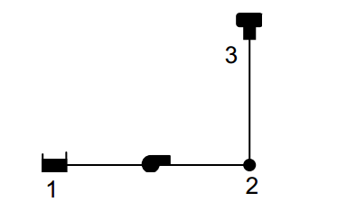
In this section, we perform thorough case studies to showcase the performance of our presented Algorithm 2 in comparison with traditional WDN control through EPANET’s built-in RBC (RBC). The simulations in this section are performed for the 3-node network in Fig. 6(a), the 8-node network in Fig. 6(b), and BWSN in Fig. 8.

We note that EPANET is a software application used to design, model, and simulate WDN [48], and it also provides RBC which has been widely employed in various engineering problems. RBC can modify the status of controllable elements based on a combination of conditions, e.g., switch on or off a pump according to the desirable safe water level in tanks.
We compare the control effort between RBC and proposed GP-MPC for the 3- and 8-node networks and BWSN. Only the comparison of control effort for the 3-node network is depicted in Fig. 7 due to space limitations, and results for the other networks are listed in Tab. VI. The weights for the three cost functions are chosen as for , for , and for .
The 3-node network in Fig. 6(a) is a simple tree network which only has one pump, one junction, and one tank. Junction 2 consumes water pumped from Reservoir 1, and the remaining water is stored in Tank 3. The control objective is to maintain the safe water level in Tank 3 defined by while minimizing pump cost and smoothness of control action. Sampling rate or control interval is set as 1 hour to avoid frequent pump switching that shortens the life of pumps [10]. After comparing the control effort of RBC in Fig. 7(a) and GP-MPC in Fig. 7(b), we note that (i) safe water level under RBC is not fully maintained for 2 hours while the safe water level under MPC is always reached; and (ii) the pump speed solved via RBC is discrete while the speed from GP-MPC and Algorithm 1 is continuous, and always remains as small as possible to reduce cost.
Objective function values are listed in Tab. VI. As previously mentioned, the objective functions are typically conflicting with each other: maintaining safe water levels and keeping smooth controls can be in conflict with achieving smaller pump speeds and hence lower electric cost of operating the pumps. The percent reductions for costs , , and are , , and for the 3-node network, which means that increases while and decrease. A similar situation also happens to BWSN, but for the 8-node network, all three objectives decrease simultaneously. The pump cost is respectively reduced by , , and for each network. The total cost is reduced by , , and for the three networks. We note that the tangible price paid by the water utility is mostly through , seeing it is difficult to quantify the monetary price of maintained safe water levels in tanks or the smoothness of control actions. With that in mind, these other two objectives ( and ) are important and should be included in a multi-period WDN control problem. Finally, we note that changing weights for the three cost functions does not change the findings: the proposed GP-MPC method outperforms RBC regardless of the weights for the cost functions .
| Network | Method | Safety: | Smoothness: | Pump cost: | Total: |
| 3-node network | RBC | ||||
| GP-MPC | |||||
| Reduced | |||||
| 8-node network | RBC | ||||
| GP-MPC | |||||
| Reduced | |||||
| BWSN | RBC | ||||
| GP-MPC | |||||
| Reduced |
VIII Limitations and Future Work
The limitations of this paper lie in the sub-optimality of the proposed heuristic. This is a result of not using integer variables to model valve and pump operations. Besides that, this paper performs the optimal control considering PRVs or FCVs assuming the settings are known, rather than optimizing the valve settings. Another limitation is the lack of explicit quantification of water demand uncertainty. Although we illustrate that the GP-based control is robust to small demand uncertainty, chance-constrained versions of the GP formulation can provide assurance in terms of robustness to uncertainty. In addition, and although empirical simulations have shown that the GP-based approximation of the nonconvex head loss models return feasible solutions regardless of the initial approximation point, a theoretical investigation of feasibility and convergence of the presented approximation is an important research direction and a limitation of this current work. Finally, exploring the performance and comparing (i) various mixed-integer and (ii) continuous, convex optimization formulations of the MPC problem in WDN is another important future research direction. Future work will address these limitations and directions.
References
- [1] H. Mala-Jetmarova, N. Sultanova, and D. Savic, “Lost in optimisation of water distribution systems? a literature review of system operation,” Environmental Modelling & Software, vol. 93, pp. 209–254, 2017.
- [2] C. Ocampo-Martinez, V. Puig, G. Cembrano, and J. Quevedo, “Application of predictive control strategies to the management of complex networks in the urban water cycle applications of control.” Institute of Electrical and Electronics Engineers, 2013.
- [3] Y. Wang, V. Puig, and G. Cembrano, “Non-linear economic model predictive control of water distribution networks,” Journal of Process Control, vol. 56, pp. 23–34, 2017.
- [4] G. S. Sankar, S. M. Kumar, S. Narasimhan, S. Narasimhan, and S. M. Bhallamudi, “Optimal control of water distribution networks with storage facilities,” Journal of Process Control, vol. 32, pp. 127–137, 2015.
- [5] N. G. Mohammed and A. Abdulrahman, “Water supply network system control based on model predictive control,” in Proceedings of the International MultiConference of Engineers and Computer Scientists, vol. 2, 2009.
- [6] G. Bonvin, S. Demassey, and A. Lodi, “Pump scheduling in drinking water distribution networks with an lp/nlp-based branch and bound,” 2019.
- [7] A. M. Gleixner, H. Held, W. Huang, and S. Vigerske, “Towards globally optimal operation of water supply networks,” 2012.
- [8] A. S. Zamzam, E. Dall’Anese, C. Zhao, J. A. Taylor, and N. Sidiropoulos, “Optimal water-power flow problem: Formulation and distributed optimal solution,” IEEE Transactions on Control of Network Systems, 2018.
- [9] M. K. Singh and V. Kekatos, “Optimal scheduling of water distribution systems,” IEEE Transactions on Control of Network Systems, pp. 1–1, 2019.
- [10] B. Ghaddar, J. Naoum-Sawaya, A. Kishimoto, N. Taheri, and B. Eck, “A lagrangian decomposition approach for the pump scheduling problem in water networks,” European Journal of Operational Research, vol. 241, no. 2, pp. 490–501, 2015.
- [11] R. Menke, E. Abraham, P. Parpas, and I. Stoianov, “Approximation of system components for pump scheduling optimisation,” Procedia Engineering, vol. 119, pp. 1059–1068, 2015.
- [12] D. Fooladivanda and J. A. Taylor, “Optimal pump scheduling and water flow in water distribution networks,” in 2015 54th IEEE Conference on Decision and Control (CDC). IEEE, 2015, pp. 5265–5271.
- [13] H. Cross, “Analysis of flow in networks of conduits or conductors,” University of Illinois at Urbana Champaign, College of Engineering. Engineering Experiment Station., Tech. Rep., 1936.
- [14] D. Martin and G. Peters, “The application of newton’s method to network analysis by digital computer,” Journal of the institute of Water Engineers, vol. 17, no. 2, pp. 115–129, 1963.
- [15] R. Epp and A. G. Fowler, “Efficient code for steady-state flows in networks,” Journal of the hydraulics division, vol. 96, no. 1, pp. 43–56, 1970.
- [16] D. J. Wood and A. Rayes, “Reliability of algorithms for pipe network analysis,” Journal of the Hydraulics Division, vol. 107, no. 10, pp. 1145–1161, 1981.
- [17] D. J. Wood and C. O. Charles, “Hydraulic network analysis using linear theory,” Journal of the Hydraulics division, vol. 98, no. 7, pp. 1157–1170, 1972.
- [18] L. T. Isaacs and K. G. Mills, “Linear theory methods for pipe network analysis,” Journal of the hydraulics division, vol. 106, no. 7, pp. 1191–1201, 1980.
- [19] M. L. Arora, “Flows split in closed loops expending least energy,” Journal of the Hydraulics Division, vol. 102, no. 3, pp. 455–458, 1976.
- [20] M. A. Collins, L. Cooper, R. Helgason, and J. Kennington, “Solution of large scale pipe networks by improved mathematical approaches,” 1978.
- [21] E. P. Todini, “S. a gradient method for the solution of looped pipe networks,” in Proceedings of the Int. Conf. on Computer Applications in Water Supply and Distribution, vol. 1, 1987.
- [22] H. Zhang, X. Cheng, T. Huang, H. Cong, and J. Xu, “Hydraulic Analysis of Water Distribution Systems Based on Fixed Point Iteration Method,” Water Resour. Manag., vol. 31, no. 5, pp. 1605–1618, Mar. 2017.
- [23] M. Bazrafshan, N. Gatsis, M. Giacomoni, and A. Taha, “A fixed-point iteration for steady-state analysis of water distribution networks,” in Proc. 6th IEEE Global Conf. Signal and Information Processing, Anaheim, CA, Nov. 2018. https://arxiv.org/abs/1807.01404
- [24] M. K. Singh and V. Kekatos, “On the flow problem in water distribution networks: Uniqueness and solvers,” arXiv preprint arXiv:1901.03676, 2019.
- [25] Y. Wang, C. Ocampo-Martinez, and V. Puig, “Stochastic model predictive control based on gaussian processes applied to drinking water networks,” IET Control Theory & Applications, vol. 10, no. 8, pp. 947–955, 2016.
- [26] A. P. Goryashko and A. S. Nemirovski, “Robust energy cost optimization of water distribution system with uncertain demand,” Automation and Remote Control, vol. 75, no. 10, pp. 1754–1769, 2014.
- [27] C. C. Sun, V. Puig, and G. Cembrano, “Combining csp and mpc for the operational control of water networks,” Engineering Applications of Artificial Intelligence, vol. 49, pp. 126–140, 2016.
- [28] G. Bonvin and S. Demassey, “Extended linear formulation of the pump scheduling problem in water distribution networks,” 2019.
- [29] J. Humpola and A. Fügenschuh, “A unified view on relaxations for a nonlinear network flow problem,” 2013.
- [30] H. D. Sherali, S. Subramanian, and G. Loganathan, “Effective relaxations and partitioning schemes for solving water distribution network design problems to global optimality,” Journal of Global Optimization, vol. 19, no. 1, pp. 1–26, 2001.
- [31] E. Salomons, A. Goryashko, U. Shamir, Z. Rao, and S. Alvisi, “Optimizing the operation of the haifa-a water-distribution network,” Journal of Hydroinformatics, vol. 9, no. 1, pp. 51–64, 2007.
- [32] M. Xie and M. Brdys, “Nonlinear model predictive control of water quality in drinking water distribution systems with dbps objectives.”
- [33] L. Sela Perelman and S. Amin, “Control of tree water networks: A geometric programming approach,” Water Resources Research, vol. 51, no. 10, pp. 8409–8430, 2015.
- [34] A. Fügenschuh and J. Humpola, A unified view on relaxations for a nonlinear network flow problem. Helmut-Schmidt-Univ., Univ. der Bundeswehr Hamburg, 2014.
- [35] D. Fooladivanda and J. A. Taylor, “Energy-optimal pump scheduling and water flow,” IEEE Transactions on Control of Network Systems, no. 3, pp. 1016–1026, Sept. 2018.
- [36] F. Pecci, E. Abraham, and I. Stoianov, “Quadratic head loss approximations for optimisation problems in water supply networks,” Journal of Hydroinformatics, vol. 19, no. 4, pp. 493–506, 2017.
- [37] J. M. Grosso, J. M. Maestre, C. Ocampo-Martinez, and V. Puig, “On the assessment of tree-based and chance-constrained predictive control approaches applied to drinking water networks.” International Federation of Automatic Control, 2014.
- [38] S. Boyd, S.-J. Kim, L. Vandenberghe, and A. Hassibi, “A tutorial on geometric programming,” Optimization and engineering, vol. 8, no. 1, p. 67, 2007.
- [39] E. Hernadez, S. Hoagland, and L. Ormsbee, “Water distribution database for research applications,” in World Environmental and Water Resources Congress 2016, 2016, pp. 465–474.
- [40] D. G. Eliades, M. Kyriakou, S. Vrachimis, and M. M. Polycarpou, “Epanet-matlab toolkit: An open-source software for interfacing epanet with matlab,” in Proc. 14th International Conference on Computing and Control for the Water Industry (CCWI), The Netherlands, Nov 2016, p. 8.
- [41] L. A. Rossman et al., “Epanet 2: users manual,” 2000.
- [42] https://github.com/ShenWang9202/GP-Based-MPC-4-WDNs
- [43] S. Wang, A. F. Taha, N. Gatsis, and M. Giacomoni, “Geometric programming-based control for nonlinear, dae-constrained water distribution networks,” in 2019 American Control Conference (ACC), July 2019, pp. 1470–1475. https://arxiv.org/pdf/1902.06026.pdf
- [44] V. Puig, C. Ocampo-Martinez, R. Pérez, G. Cembrano, J. Quevedo, and T. Escobet, Real-Time Monitoring and Operational Control of Drinking-Water Systems. Springer, 2017.
- [45] R. K. Linsley and J. B. Franzini, Water-resources engineering. McGraw-Hill New York, 1979, vol. 165.
- [46] R. Menke, E. Abraham, and I. Stoianov, “Modeling variable speed pumps for optimal pump scheduling,” in World Environmental and Water Resources Congress 2016, 2016, pp. 199–209.
- [47] D. E. Knuth, The art of computer programming: sorting and searching. Pearson Education, 1997, vol. 3.
- [48] E. P. Agency, “Epanet.” https://www.epa.gov/water-research/epanet
- [49] A. Mutapcic, K. Koh, S. Kim, L. Vandenberghe, and S. Boyd, “Ggplab: A simple matlab toolbox for geometric programming,” web page and software: http://stanford. edu/boyd/ggplab, 2006.
Appendix A GP Background and Definitions
A geometric program is a type of optimization problem with objectives and constraint functions that are monomials and posynomials [38]. A real valued function , where and , is called a monomial of the variables . A sum of one or more monomials, i.e., a function of the form where , is called a posynomial with terms in the vector variable . A standard GP can be written as
| (30) | ||||
where is an entry-wise positive optimization variable, are posynomial functions and are monomials. The definitions given next are used in the paper.
Definition 1.
For matrices and , the element-wise exponential operation on with base , denoted as , is a matrix of the same dimension with elements given by
When , where is an matrix of all ones, can be denoted as for simplicity. When , can be denoted as for simplicity, which can be viewed as element-wise power of matrix .
Definition 2.
For matrices and matrix , the element-wise exponential matrix product has elements given by for and , where .
Property 1.
For matrices with size and with size , let , where is base. The following holds:
Example 1.
For matrices
Appendix B Closed-form Expression of
We now provide the closed-form expression of from (24). This function can be written as
| (31a) | ||||
| (31b) | ||||
| (31c) | ||||
| (31d) | ||||
| (31e) | ||||
as column vectors respectively collecting all of parameters and of pumps where are submatrices after splitting (18c), , , , and are column vectors collecting all the , , and . Equations (31c), (31d), and (31e) are the abstract GP form of pipe, pump, and valve models. The operator is the element-wise product of two matrices. All of the above state-space matrices in (31) can be generated automatically from our Github code [42].
Appendix C WDN parameters and Experimental Setup
This appendix contains all of the information needed to reproduce the results shown in the paper. The BWSN network topology, (forecast/real) water demand curves, and variable-speed pump curves are given first in Fig. 8 and Fig. 9. The basic parameters in the 126-node network including the elevation of nodes, length, and diameter of pipes are obtained from [40]. We now present the list of constraints and parameters used in the simulations.
The initial head of Tank 130 is , the water level range of Tank 130 is , and the safe water level (20a) of Tank 130 from Section III is set to . Similarly, the initial head of Tank 131 is , the water level range of Tank 131 is , and the corresponding safe water level is set to . We set the total simulation time to 24 hours in Algorithm 1.
The demand pattern for 24 hours at different junctions is shown in Fig. 9(a). This demand pattern is different from [40], as our intention is to make the demand vary more rapidly to test the performance of the presented GP-based control. In order to test the ability of handling uncertainty, our algorithm only uses the demand forecast whereas the EPANET simulator uses the real demand shown in Fig. 9(a). The real demand and forecast are randomly generated with difference.
The relationship between head increase and flow of Pump 170 and Pump 172 defined by (7) are presented in Fig. 9(b). We observe that the head increase and flow provided by a pump varies with the relative speed with referring to the pump being off and the constraints (7) should be removed from GP-MPC as we discussed in Section II-B. Pump 170 is used with shutoff head , , and ; the corresponding parameters of Pump 172 are , , and . The default global efficiency is for all pumps in [40] and the efficiency curves of pumps are not specified. But in practice, the pump efficiency is dynamic, and is considered while calculating the pump cost in (21). Hence, we define the efficiency curves of Pump 170 and Pump 172 in Fig. 9(b).
In (15), the physical constraints of the head imposed at the junction is greater than its corresponding elevation, and the head of reservoir is fixed at its elevation. Since we have only one reservoir, this implies that . As for the flow, the direction is unknown, and we simply constrain the flow to .
For the geometric programming component of the presented formulations, we set the base . The parameters we use in Algorithm 2 are selected as: and . We consider a sampling time of , a prediction horizon . For a single MPC window, GP-MPC has 2177 variables, 2283 constraints and takes approximately to find the final solution at and the computational time for entire simulation is .
The numerical tests are simulated using EPANET Matlab Toolkit [40] on Ubuntu 16.04.4 LTS with an Intel(R) Xeon(R) CPU E5-1620 v3 @ 3.50GHz. The GP solver used here is GGPLAB [49]. All codes and figures are included in [42].
![[Uncaptioned image]](1909.03181v3/Shen.png) |
Shen Wang received the master’s degree in Control Science and Engineering from the University of Science and Technology of China, Hefei, China, in 2016. He is currently pursuing a Ph.D. degree in Electrical Engineering at the University of Texas at San Antonio, Texas. His current research interests include optimal control in cyber-physical systems with special focus on energy and water systems. |
![[Uncaptioned image]](1909.03181v3/Taha.png) |
Ahmad F. Taha is an assistant professor with the Department of Electrical and Computer Engineering at the University of Texas, San Antonio. He received the B.E. and Ph.D. degrees in Electrical and Computer Engineering from the American University of Beirut, Lebanon in 2011 and Purdue University, West Lafayette, Indiana in 2015. Dr. Taha is interested in understanding how complex cyber-physical systems (CPS) operate, behave, and misbehave. His research focus includes optimization, control, and security of CPSs with applications to power, water, and transportation networks. Dr. Taha is an editor of IEEE Transactions on Smart Grid and the editor of the IEEE Control Systems Society Electronic Letter (E-Letter). |
![[Uncaptioned image]](1909.03181v3/Gatsis.jpg) |
Nikolaos Gatsis received the Diploma degree in Electrical and Computer Engineering from the University of Patras, Greece, in 2005 with honors. He completed his graduate studies at the University of Minnesota, where he received the M.Sc. degree in Electrical Engineering in 2010, and the Ph.D. degree in Electrical Engineering with minor in Mathematics in 2012. He is currently an Associate Professor with the Department of Electrical and Computer Engineering at the University of Texas at San Antonio. His research focuses on optimal and secure operation of smart power grids and other critical infrastructures, including water distribution networks and the Global Positioning System. Dr. Gatsis is a recipient of the NSF CAREER award. He has co-organized symposia in the area of smart grids in IEEE GlobalSIP 2015 and 2016. He has also served as a co-guest editor for a special issue of the IEEE Journal on Selected Topics in Signal Processing on Critical Infrastructures. |
![[Uncaptioned image]](1909.03181v3/Marcio.jpg) |
Marcio H. Giacomoni is an associate professor in Civil and Environmental Engineering at the University of Texas at San Antonio. He earned his bachelor’s degree in Civil Engineering from the University of Brasilia and a master’s of science in Water Resources from the Institute of Hydraulics Research at the Federal University of Rio Grande do Sul, Brazil. He obtained his Ph.D. in Civil Engineering from Texas A&M University. His long-term goal is to develop and sustain a career as a teacher-scholar focused on methodologies that identify smart water planning and management strategies that enhance the sustainability and resilience of the built and natural environments, and transform this knowledge into action by training the next generation of water planners and managers with state-of-the-art knowledge and tools. |