跳到论文正文
W Papers独立论文阅读器 arXiv:1909.03007 论文正文 计算阅读时间 · 0%
引用这篇论文根据当前论文元数据生成,正式投稿前建议核对。


License: arXiv.org perpetual non-exclusive license
arXiv:1909.03007v2 [hep-th] 10 Feb 2020

CPHT-RR046.072019

DESY 19-125

Quantum corrections for D-brane models
with broken supersymmetry

Wilfried Buchmuller†11 1 E-mail: wilfried.buchmueller@desy.de, Emilian Dudas∗22 2 E-mail: emilian.dudas@cpht.polytechnique.fr, Yoshiyuki Tatsuta†33 3 E-mail: yoshiyuki.tatsuta@desy.de

† Deutsches Elektronen-Synchrotron DESY, 22607 Hamburg, Germany

∗ CPHT, CNRS, Institute Polytechnique de Paris, France

Abstract

Intersecting D-brane models and their T-dual magnetic compactifications yield attractive models of particle physics where magnetic flux plays a twofold role, being the source of fermion chirality as well as supersymmetry breaking. A potential problem of these models is the appearance of tachyons which can only be avoided in certain regions of moduli space and in the presence of Wilson lines. We study the effective four-dimensional field theory for an orientifold compactification of type IIA string theory and the corresponding toroidal compactification of type I string theory. After determining the Kaluza-Klein and Landau-level towers of massive states in different sectors of the model, we evaluate their contributions to the one-loop effective potential, summing over all massive states, and we relate the result to the corresponding string partition functions. We find that the Wilson-line effective potential has only saddle points, and the theory is therefore driven to the tachyonic regime. There tachyon condensation takes place and chiral fermions acquire a mass of the order of the compactification scale. We also find evidence for a tachyonic behaviour of the volume moduli. More work on tachyon condensation is needed to clarify the connection between supersymmetry breaking, a chiral fermion spectrum and vacuum stability.

1 Introduction

Intersecting D-brane models and their T-dual magnetic compactifications provide attractive and intuitive string theory compactifications to four dimensions with chiral fermion spectra [1, 2]. The main emphasis in model building has been on the construction of vacua with unbroken 𝒩=1\mathcal{N}=1 supersymmetry (for a review and references, see [3, 4]), but in absence of any hint for supersymmetry at the Large Hadron Collider, models where supersymmetry is broken at a high scale, in the spirit of ‘split supersymmetry’ [5, 6] or ‘split symmetries’ [7, 8], are also of current interest.

An intriguing aspect of magnetic compactifications is the connection between fermion chirality and supersymmetry breaking [9], which occurs in compactifications of type I strings on tori and orbifolds [10, 11, 12] and in the related intersecting D-brane models [13, 11, 14]. This setup allows to construct models which come very close to the Standard Model of particle physics [15, 16, 17, 18]. Generically, magnetic compactifications have tachyonic instabilities of Nielsen-Olesen type [19]. Originally, one could hope to relate such an instability to electroweak symmetry breaking [9, 15, 16] in case of a low string scale and large extra dimensions. This is no longer viable but the structure of the setup is rich enough to incorporate in principle also split supersymmetry [20, 21].

The goal of this paper is the computation of quantum corrections for string compactifications with magnetic background flux. This is partly motivated by the recent observation that in quantum corrections to Wilson-line scalars large cancellations occur [22, 23, 24, 25] due to the presence of magnetic flux. This suggests that in appropriate compactifications similar cancellations may occur in quantum corrections to Higgs masses, which would be important in view of the hierarchy problem. In order to address these questions we extend the previous calculations for six-dimensional field theory models to a full string compactification on magnetized tori. Notice, that another motivation of our effective field theory approach is that, whenever supersymmetry is broken by magnetic fluxes, in string theory NSNS tadpoles are generated that make any quantum computation very hard, both conceptually and technically (see, for example, [26]).

Our starting point is the construction of an intersecting brane model with broken supersymmetry in a matter sector without tachyons and with chiral fermions which can acquire mass via the Higgs mechanism. For simplicity, and to facilitate the computation of quantum corrections, we choose as unbroken gauge group U⁡(N)×U⁡(1)×U⁡(1)U(N)\times U(1)\times U(1) rather than the Standard Model gauge group. The model has a Higgs sector and antisymmetric tensor fields with fermions in vector-like representations. Some scalar masses in these sectors depend on the distance between branes that are parallel in some tori. These moduli correspond to Wilson-line scalars in the T-dual picture. They become tachyonic if the branes come close to each other. At tree level the Wilson-line potential is flat. However, as we shall see, one-loop quantum corrections make it concave, implying that the system is driven into the tachyonic regime of moduli space.

After determining intersection numbers and scalar masses for the D-brane model, we turn to the T-dual magnetic compactification which is better suited to evaluate the four-dimensional (4d) effective field theory. Starting from the 10d S​O​(32)SO(32) Super-Yang-Mills Lagrangian expressed in terms of 𝒩=1\mathcal{N}=1 vector and chiral superfields [27, 28], we compute the 4d effective action for a toroidal compactification with three U⁡(1)U(1) magnetic background fluxes that break S​O​(32)SO(32) to U⁡(N)×U⁡(1)×U⁡(1)U(N)\times U(1)\times U(1). For each sector of the model we determine the Kaluza-Klein (KK) and Landau-level (LL) towers of mass eigenstates of vectors, fermions and scalars. The calculations are based on the harmonic oscillator algebra of covariant derivatives in a flux background [9, 29, 30, 31, 24]. The mass spectra are compared with the string formula of Bachas, also in view of supersymmetries that remain unbroken for particular choices of magnetic fluxes in some sectors.

In the Higgs sector branes are parallel in some tori and, knowing the spectrum of massive KK and LL states, we compute the effective potential as function of magnetic flux and Wilson lines. The effective potential is also obtained in the field theory limit of the corresponding string partition function, and the two results agree. As function of the Wilson line the potential is concave and there are no local minima. Hence, the tree level vacua with non-vanishing Wilson lines are unstable. This is a new result of our paper. For vanishing Wilson lines tachyon condensation takes place and all chiral fermions acquire masses of the order of the compactification scale.

The contributions to the effective potential from the various sectors are most easily obtained from the corresponding string partition functions. In sectors without Wilson lines we also calculate the effective potential as function of the volume moduli of the three tori. We find evidence that also in this case the system is driven to the tachyonic regime of moduli space, which would imply that the only vacuum state corresponds to the decompactification limit. A further, well-known problem is the NSNS tadpole (see, for example, [26]) in case of broken supersymmetry.

The paper is organized as follows. The intersecting D-brane model and its T-dual magnetic compactification are discussed in Sections 2 and 3, respectively. Mass eigenstates and mass spectra are derived in Sections 4 and 5, and the effective one-loop potential is computed in Section 6. Section 7 deals with tachyon condensation. The appendices A and B give details concerning the embedding of the various sectors of the model in the adjoint representation of S​O​(32)SO(32), and in the appendices C and D some formulae are collected for superfield components and Jacobi functions, respectively.

2 Intersecting D-brane model

We are interested in a D-brane model with broken supersymmetry, which contains a ‘matter sector’ with chiral fermions and a ‘Higgs sector’ with vector-like fermions such that vacuum expectation values of Higgs fields can give mass to the chiral fermions. As a simple example, we choose the gauge group

G=U⁡(N)×U⁡(1)×U⁡(1),\displaystyle G=U(N)\times U(1)\times U(1)\ , (1)

corresponding to a stack of NN branes, aa, and two single branes, bb and cc. The fermions are supposed to be chiral with respect to U⁡(1)×U⁡(1)U(1)\times U(1) and vector-like with respect to the ‘colour group’ U⁡(N)U(N). Following [11, 16], we start from type IIA string theory compactified on a rectangular factorized torus T6=T12×T22×T32T^{6}=T^{2}_{1}\times T^{2}_{2}\times T^{2}_{3} with real coordinates x4,…,x9x_{4},\ldots,x_{9} and complex coordinates zi=(x2+2​i+i​x3+2​i)/2z_{i}=(x_{2+2i}+ix_{3+2i})/2, i=1,2,3i=1,2,3, with the identifications zi∼zi+Li/2z_{i}\sim z_{i}+L_{i}/2, zi∼zi+i​Li′/2z_{i}\sim z_{i}+iL^{\prime}_{i}/2. An orientifold is obtained by dividing out the discrete symmetry Ω​ℛ​(−1)FL\Omega\mathcal{R}(-1)^{F_{L}}, where Ω\Omega is worldsheet parity, FLF_{L} is left-moving fermion number, and ℛ\mathcal{R} is a reflection symmetry of T6T^{6},

ℛ:(z1,z2,z3)→(z¯1,z¯2,z¯3).\displaystyle\mathcal{R}:(z_{1},z_{2},z_{3})\rightarrow(\bar{z}_{1},\bar{z}_{2},\bar{z}_{3})\ . (2)

The orientifold has eight O​6O6-planes along Minkowski space and the directions x3+2​ix_{3+2i} that are invariant under ℛ\mathcal{R}. The orientifold planes are localized at the fixed points (z^1,z^2,z^3)(\hat{z}_{1},\hat{z}_{2},\hat{z}_{3}), z^i=(0,i​L′/4)\hat{z}_{i}=(0,iL^{\prime}/4). Each orientifold plane has RR charge QO​6=−2Q_{O6}=-2 in units of a D6-brane charge.

Branes, gauge groups (n1,m1)(n^{1},m^{1}) (n2,m2)(n^{2},m^{2}) (n3,m3)(n^{3},m^{3})
a,U⁡(N)a\ ,\ U(N) (1,0)(1,0) (1,2)(1,2) (1,1)(1,1)
b,U⁡(1)b\ ,\ U(1) (1,1)(1,1) (1,l)(1,l) (1,−2)(1,-2)
c,U⁡(1)c\ ,\ U(1) (1,1)(1,1) (1,−l)(1,-l) (1,2)(1,2)
Table 1: Intersecting D-brane model. Wrapping numbers of a stack of NN branes, aa, and two single branes, bb and cc.

Cancellation of the total RR charge requires 16 D6-branes together with 16 mirror D6 branes to satisfy the reflection symmetry ℛ\mathcal{R} of the compact space. A brane ee is wrapped around the 1-cycles [ai][a_{i}] and [bi][b_{i}] of the 2-tori Ti2T^{2}_{i} with wrapping numbers nein_{e}^{i} and meim_{e}^{i}, yielding for the wrapped 3-cycle of the brane the homology class11 1 We mostly follow the conventions of [4].

[Πe]=⊗i(nei[ai]+mei[bi]).\displaystyle[\Pi_{e}]=\otimes_{i}\left(n^{i}_{e}[a_{i}]+m^{i}_{e}[b_{i}]\right)\ . (3)

The homology class [Πe′][\Pi_{e^{\prime}}] of the mirror brane is obtained from [Πe][\Pi_{e}] by replacing meim^{i}_{e} by −mei-m^{i}_{e}. In case of stacks of NeN_{e} branes, leading to gauge symmetries U⁡(Ne)U(N_{e}), the RR tadpole cancellation condition can now be written as

∑eNe​[Πe]−2​[ΠO​6]=0,\displaystyle\sum_{e}N_{e}[\Pi_{e}]-2[\Pi_{O6}]=0\ , (4)

where [ΠO​6]=8⊗i[ai][\Pi_{O6}]=8\otimes_{i}[a_{i}] is the homology class of the orientifold plane.

We are interested in the gauge group U⁡(N)×U⁡(1)×U⁡(1)U(N)\times U(1)\times U(1), corresponding to one stack of NN branes, aa, with gauge group U⁡(N)U(N), and two further single U⁡(1)U(1) branes, bb and cc. Table 1 shows a set of wrapping numbers which can be consistent with the wanted gauge group U⁡(N)×U⁡(1)×U⁡(1)U(N)\times U(1)\times U(1). We have chosen all wrapping number in the x3+2​ix_{3+2i} directions equal, ni=1n^{i}=1, and one wrapping number in the first torus as zero, ma1=0m^{1}_{a}=0. In this case, the tadpole conditions (4) read explicitly,

N+2=16,N​ma2​ma3+mb2​mb3+mc2​mc3=0,mb1​mb3+mc1​mc3=0,mb1​mb2+mc1​mc2=0.\begin{split}N+2&=16\ ,\\ Nm^{2}_{a}m^{3}_{a}+m_{b}^{2}m^{3}_{b}+m_{c}^{2}m^{3}_{c}&=0\ ,\\ m_{b}^{1}m^{3}_{b}+m_{c}^{1}m^{3}_{c}&=0\ ,\\ m_{b}^{1}m^{2}_{b}+m_{c}^{1}m^{2}_{c}&=0\ .\end{split} (5)
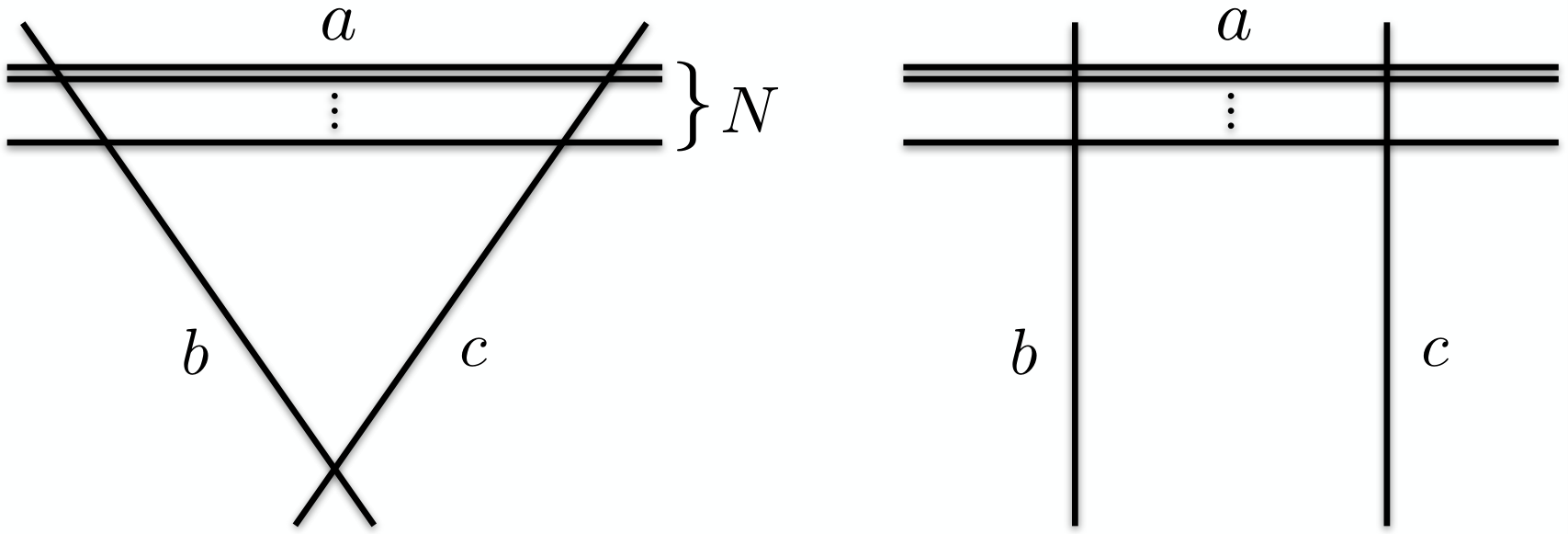
Refer to caption
Figure 1: Left: intersections of brane stack aa with branes bb and cc, and brane bb with cc in the second torus T22T^{2}_{2}; right: intersections of brane stack aa with branes bb and cc in torus T12T^{2}_{1} where branes bb and cc are parallel.

One easily verifies that these equations are solved by the ansatz in Table 1, with N=14N=14, l=7l=7. The chosen wrapping numbers imply that not all branes intersect in all tori: aa and a′a^{\prime}, and bb and cc are parallel in the first torus, whereas bb and c′c^{\prime} are parallel in the second and in the third torus. This situation is illustrated in Figure 1.

On each brane an 𝒩=4\mathcal{N}=4 supermultiplet of zero-modes in the adjoint representation of the gauge group is localized. The branes intersect at angles determined by the wrapping numbers. At these intersections fermions and scalars in bi-fundamental representations (Ne,N¯f)(N_{e},\bar{N}_{f}) are localized. For non-zero intersection numbers

Ie​f=⊗i(neimfi−meinfi)\displaystyle I_{ef}=\otimes_{i}\left(n^{i}_{e}m^{i}_{f}-m^{i}_{e}n^{i}_{f}\right) (6)

the fermion spectrum is chiral. The fermions are left-handed for Ie​f>0I_{ef}>0 and right-handed for Ie​f<0I_{ef}<0, corresponding to left-handed fermions in the complex conjugate representation (N¯e,Nf)(\bar{N}_{e},N_{f}).

Brane sector Intersection number II 4d fermions (L)
a​b+b​aab+ba −3​(l−2)-3(l-2) N¯1,0\bar{N}_{1,0}
a​c+c​aac+ca −(l+2)-(l+2) N¯0,1\bar{N}_{0,1}
a​b′+b′​aab^{\prime}+b^{\prime}a l+2l+2 N1,0{N}_{1,0}
a​c′+c′​aac^{\prime}+c^{\prime}a 3​(l−2)3(l-2) N0,1{N}_{0,1}
a​a′aa^{\prime} 00 N⁡(N−1)/2N(N-1)/2, N¯​(N¯−1)/2\bar{N}(\bar{N}-1)/2
b​c+c​bbc+cb 00 11,−11_{1,-1}, 1−1,11_{-1,1}
b​c′+c′​bbc^{\prime}+c^{\prime}b 00 11,11_{1,1}, 1−1,−11_{-1,-1}
Table 2: Chiral and vector-like representations of left-handed fermions at various brane intersections.

At the intersections of the brane system defined in Table 1 one obtains the left-handed fermions listed in Table 2. There are matter fields that carry ‘colour’, transforming as NN or N¯\bar{N} under S​U​(N)SU(N). They form a chiral representation of the full gauge group, whereas colour singlet ‘Higgs fields’ form vector-like representations. The quantum numbers of the chiral fermions allow Yukawa couplings that are most conveniently expressed in terms of the associated chiral superfields,

ℒY⊃∑r,s3​(l−2)yr​s(1)​𝑵¯1,0r​𝑵0,1s​𝟏−1,−1+∑r,sl+2yr​s(2)​𝑵¯0,1r​𝑵1,0s​𝟏−1,−1.\displaystyle\mathcal{L}_{Y}\supset\sum_{r,s}^{3(l-2)}y^{(1)}_{rs}\bm{\bar{N}}^{r}_{1,0}\bm{N}^{s}_{0,1}\bm{1}_{-1,-1}+\sum_{r,s}^{l+2}y^{(2)}_{rs}\bm{\bar{N}}^{r}_{0,1}\bm{N}^{s}_{1,0}\bm{1}_{-1,-1}\ . (7)

These couplings lead to fermion mass terms after a vacuum expectation value ⟨1−1,−1⟩≠0\langle 1_{-1,-1}\rangle\neq 0 breaks the chiral group U⁡(1)×U⁡(1)U(1)\times U(1) to the diagonal U⁡(1)U(1) subgroup. The complete list of Yukawa couplings will be given in the subsequent section.

In the brane sector a​a′aa^{\prime}, b​b′bb^{\prime} and c​c′cc^{\prime} chiral fermions in symmetric and antisymmetric representations of the gauge group occur with multiplicities

nsym,e=12​(Ie​e′−Ie,O​6)=−4​me1​me2​me3​(ne1​ne2​ne3−1),nasym,e=12(Ie​e′+Ie,O​6)=−4m1em2em3e(n1en2en3e+1),e=a,b,c.\begin{split}n_{\text{sym},e}&=\frac{1}{2}\left(I_{ee^{\prime}}-I_{e,O6}\right)=-4m^{1}_{e}m^{2}_{e}m^{3}_{e}\left(n^{1}_{e}n^{2}_{e}n^{3}_{e}-1\right)\ ,\\ n_{\text{asym},e}&=\frac{1}{2}\left(I_{ee^{\prime}}+I_{e,O6}\right)=-4m^{1}_{e}m^{2}_{e}m^{3}_{e}\left(n^{1}_{e}n^{2}_{e}n^{3}_{e}+1\right),\;e=a,b,c\ .\end{split} (8)

Since in our model ma1=0m^{1}_{a}=0 and ne1=ne2=ne3=1n^{1}_{e}=n^{2}_{e}=n^{3}_{e}=1 for e=a,b,ce=a,b,c, there are no chiral fermions in symmetric or antisymmetric representations. As we shall see in the following section, a vector-like pair of fermions in the antisymmetric representation of S​U​(N)SU(N) occurs in the a​a′aa^{\prime}-sector. The b​b′bb^{\prime}- and the c​c′cc^{\prime}-sector correspond to U⁡(1)U(1) symmetries where such representations are absent.

The masses of bi-fundamental scalars depend on the angles at which the branes intersect. We restrict ourselves to small angles with respect to the orientifold planes,

tanθie=mieρi≃θie,ρi=Li′Li,i=1,2,3,e=a,b,c,\displaystyle\tan{\theta^{i}_{e}}=m^{i}_{e}\rho_{i}\simeq\theta^{i}_{e}\ ,\quad\rho_{i}=\frac{L^{\prime}_{i}}{L_{i}}\ ,\ i=1,2,3\ ,\ e=a,b,c\ , (9)

where Li/(2​π)L_{i}/(2\pi) and Li′/(2​π)L^{\prime}_{i}/(2\pi) are the two radii of the torus Ti2T^{2}_{i}, respectively. In the T-dual picture small angles correspond to large areas of the dual tori so that we shall be able to use a field theory approximation to string partition functions.

At the intersection of two stacks of branes, ee and ff, one then has three light bi-fundamental scalars with masses [14]

4​π​α′​M12|e​f=−|θe​f1|+|θe​f2|+|θe​f3|4​π​α′​M22|e​f=|θe​f1|−|θe​f2|+|θe​f3|4​π​α′​M32|e​f=|θe​f1|+|θe​f2|−|θe​f3|,\begin{split}4\pi\alpha^{\prime}M^{2}_{1}|_{ef}&=-|\theta^{1}_{ef}|+|\theta^{2}_{ef}|+|\theta^{3}_{ef}|\\ 4\pi\alpha^{\prime}M^{2}_{2}|_{ef}&=|\theta^{1}_{ef}|-|\theta^{2}_{ef}|+|\theta^{3}_{ef}|\\ 4\pi\alpha^{\prime}M^{2}_{3}|_{ef}&=|\theta^{1}_{ef}|+|\theta^{2}_{ef}|-|\theta^{3}_{ef}|\ ,\end{split} (10)

where θe​fi=θei−θfi\theta^{i}_{ef}=\theta^{i}_{e}-\theta^{i}_{f}, with −π/2≤θie​f≤π/2-\pi/2\leq\theta^{i}_{ef}\leq\pi/2. For the model defined in Table 1 one obtains

θa1\displaystyle\theta^{1}_{a} =0,\displaystyle=0\ , θa2\displaystyle\theta^{2}_{a} =2​ρ2,\displaystyle=2\rho_{2}\ , θa3\displaystyle\theta^{3}_{a} =ρ3,\displaystyle=\rho_{3}\ ,
θb1\displaystyle\theta^{1}_{b} =ρ1,\displaystyle=\rho_{1}\ , θb2\displaystyle\theta^{2}_{b} =l​ρ2,\displaystyle=l\rho_{2}\ , θb3\displaystyle\theta^{3}_{b} =−2​ρ3,\displaystyle=-2\rho_{3}\ ,
θc1\displaystyle\theta^{1}_{c} =ρ1,\displaystyle=\rho_{1}\ , θc2\displaystyle\theta^{2}_{c} =−l​ρ2,\displaystyle=-l\rho_{2}\ , θc3\displaystyle\theta^{3}_{c} =2​ρ3.\displaystyle=2\rho_{3}\ . (11)

Using Eq. (10) these angles yield the scalar mass spectrum at the various brane intersections which is listed in Table 3.

Brane sectors 4​π​α′​M12|e​f4\pi\alpha^{\prime}M_{1}^{2}|_{ef} 4​π​α′​M22|e​f4\pi\alpha^{\prime}M_{2}^{2}|_{ef} 4​π​α′​M32|e​f4\pi\alpha^{\prime}M_{3}^{2}|_{ef}
a​b,a​c′ab,ac^{\prime} −ρ1+(l−2)​ρ2+3​ρ3-\rho_{1}+(l-2)\rho_{2}+3\rho_{3} ρ1−(l−2)​ρ2+3​ρ3\rho_{1}-(l-2)\rho_{2}+3\rho_{3} ρ1+(l−2)​ρ2−3​ρ3\rho_{1}+(l-2)\rho_{2}-3\rho_{3}
a​b′,a​cab^{\prime},ac −ρ1+(l+2)​ρ2+ρ3-\rho_{1}+(l+2)\rho_{2}+\rho_{3} ρ1−(l+2)​ρ2+ρ3\rho_{1}-(l+2)\rho_{2}+\rho_{3} ρ1+(l+2)​ρ2−ρ3\rho_{1}+(l+2)\rho_{2}-\rho_{3}
a​a′aa^{\prime} 4​ρ2+2​ρ34\rho_{2}+2\rho_{3} −4​ρ2+2​ρ3-4\rho_{2}+2\rho_{3} 4​ρ2−2​ρ34\rho_{2}-2\rho_{3}
b​cbc 2​l​ρ2+4​ρ32l\rho_{2}+4\rho_{3} −2​l​ρ2+4​ρ3-2l\rho_{2}+4\rho_{3} 2​l​ρ2−4​ρ32l\rho_{2}-4\rho_{3}
b​c′bc^{\prime} −2​ρ1-2\rho_{1} 2​ρ12\rho_{1} 2​ρ12\rho_{1}
Table 3: Masses of scalars at various brane intersections.

In any sector of states stretched between any two stacks of branes ee, ff, some supersymmetry is preserved provided that angles fulfill the following conditions [13],

θe​f1±θe​f2±θe​f3≠0:𝒩=4→𝒩=0,\displaystyle\theta_{ef}^{1}\pm\theta_{ef}^{2}\pm\theta_{ef}^{3}\not=0\ :\quad\hskip 19.91684pt{\cal N}=4\to{\cal N}=0\ ,
θe​f1±θe​f2±θe​f3=0:𝒩=4→𝒩=1,\displaystyle\theta_{ef}^{1}\pm\theta_{ef}^{2}\pm\theta_{ef}^{3}=0\ :\quad\hskip 19.91684pt{\cal N}=4\to{\cal N}=1\ ,
θe​f1±θe​f2=0,θe​f3=0:𝒩=4→𝒩=2.\displaystyle\theta_{ef}^{1}\pm\theta_{ef}^{2}=0\ ,\;\theta_{ef}^{3}=0\ :\quad{\cal N}=4\to{\cal N}=2\ . (12)

In the considered model, a tachyon occurs in the b​c′bc^{\prime}-sector,

m12|b​c′∝−2​ρ1<0.\displaystyle m^{2}_{1}|_{bc^{\prime}}\propto-2\rho_{1}<0\ . (13)

A further tachyon appears either in the a​a′aa^{\prime}-sector or in the b​cbc-sector. In both sectors the flux in the first torus is zero, i.e. θ1=0\theta^{1}=0. Choosing θ2=θ3\theta^{2}=\theta^{3} yields two massless scalars, avoiding tachyons. For the a​a′aa^{\prime}-sector this means

ρ3=2​ρ2,\displaystyle\rho_{3}=2\rho_{2}\ , (14)

which avoids coloured tachyons but implies a second tachyon in the b​cbc-sector,

m12|b​c∝(−2​l+4)​ρ2<0.\displaystyle m^{2}_{1}|_{bc}\propto(-2l+4)\rho_{2}<0\ . (15)

Together with the two fermionic zero-modes the a​a′aa^{\prime}-sector then forms a subsystem with 𝒩=2\mathcal{N}=2 supersymmetry. For the choice l​ρ2=2​ρ3l\rho_{2}=2\rho_{3} the roles the a​a′aa^{\prime}-sector and the b​cbc-sector are reversed.

The condition for absence of tachyons in the a​bab- and a​c′ac^{\prime}-sector reads

(8−l)​ρ2<ρ1<(l+4)​ρ2,\displaystyle(8-l)\rho_{2}<\rho_{1}<(l+4)\rho_{2}\ , (16)

and for the a​b′ab^{\prime}- and a​cac-sector one obtains

l​ρ2<ρ1<(l+4)​ρ2.\displaystyle l\rho_{2}<\rho_{1}<(l+4)\rho_{2}\ . (17)

With l=7l=7, the last condition (17) is the stronger one and implies condition (16). Hence, once the conditions (14) and (17) are satisfied, all scalars in the sectors a​bab, a​c′ac^{\prime}, a​b′ab^{\prime} and a​cac are massive and supersymmetry is completely broken. The angles satisfying these conditions form a tetrahedron [16]. It is illustrated in Figure 2, together with a domain of small angles.

Refer to caption
Figure 2: Domain of angles for which no tachyons appear. Left: line in θ2−θ3\theta^{2}-\theta^{3}-plane in case of no flux in first torus, i.e. θ1=0\theta^{1}=0. Right: tetrahedron in case of fluxes in all tori. The gray areas indicate small-angle domains with |θi|/π<0.15|\theta^{i}|/\pi<0.15.

The appearance of tachyons is a generic feature of non-supersymmetric intersecting D-brane models. However, it is argued that such tachyons can be removed by couplings to moduli fields that parametrize the distance between branes in tori where they are parallel. In the T-dual picture discussed in the following section these moduli correspond to Wilson-lines ξ\xi, ξ′\xi^{\prime} that acquire vacuum expectation values (see, for example, [16, 21]). In the present model the corresponding superpotential terms would have the form (in superfield notation, see Table 2),

Wξ,ξ′=λ1​ξ​𝟏1,−1​𝟏−1,1+λ2​ξ′​𝟏1,1​𝟏−1,−1.\displaystyle W_{\xi,\xi^{\prime}}=\lambda_{1}~\xi~\mathbf{1}_{1,-1}\mathbf{1}_{-1,1}+\lambda_{2}~\xi^{\prime}~\mathbf{1}_{1,1}\mathbf{1}_{-1,-1}\ . (18)

Clearly, existence and stability of a ground state require an appropriate potential for ξ\xi, ξ′\xi^{\prime}. At tree-level the potential is flat. To compute the one-loop quantum correction to the potential is an essential goal of this paper. To achieve this we first construct the T-dual type I string compactification on a magnetized torus, which allows a straightforward computation of the full mass spectrum of the model as well as Yukawa couplings.

3 T-dual toroidal flux compactification

The intersecting D-brane model constructed in the previous section is T-dual to a type I compactification on a magnetized dual rectangular torus T12×T22×T32T^{2}_{1}\times T^{2}_{2}\times T^{2}_{3} with the identifications

zi∼zi+Li/2,zi∼zi+2​π2​α′/Li′,\displaystyle z_{i}\sim z_{i}+L_{i}/2\ ,\quad z_{i}\sim z_{i}+2\pi^{2}\alpha^{\prime}/L^{\prime}_{i}\ , (19)

where the angles θei\theta^{i}_{e} between brane ee and the orientifold plane are related to magnetic flux densities in the 2-tori Ti2T^{2}_{i} [13],

tan⁡θei=2​π​α′​g​fIi.\displaystyle\tan\theta^{i}_{e}=2\pi\alpha^{\prime}gf^{i}_{I}\ . (20)

Here gg is the gauge coupling, brane ee (e=a,b,ce=a,b,c) has a U⁡(1)U(1) group with Cartan generator HIH_{I} (I=0,1,2I=0,1,2), and fIif^{i}_{I} is the corresponding flux density in the torus Ti2T^{2}_{i}. Using Eq. (9), tan⁡θei=mIi​ρi\tan{\theta^{i}_{e}}=m^{i}_{I}\rho_{i}, this implies the Dirac quantization condition for the flux densities fIif^{i}_{I},

g​∫Ti2fIi=4​π2​α′ρi​g​fIi=2​π​mIi.\displaystyle g\int_{T^{2}_{i}}f^{i}_{I}=\frac{4\pi^{2}\alpha^{\prime}}{\rho_{i}}gf^{i}_{I}=2\pi m^{i}_{I}\ . (21)

For small angles, corresponding to small flux densities, one has22 2 In the following we shall use the notations feif^{i}_{e}, meim^{i}_{e} and fIif^{i}_{I}, mIim^{i}_{I} in parallel, according to convenience.

θei≃mIi​ρi=2​π​α′​g​fIi,ρi=Li′/Li.\displaystyle\theta^{i}_{e}\simeq m^{i}_{I}\rho_{i}=2\pi\alpha^{\prime}gf^{i}_{I}\ ,\quad\rho_{i}=L^{\prime}_{i}/L_{i}\ . (22)

The considered D-brane model has three stacks of branes and therefore three U⁡(1)U(1) factors, U​(1)aU(1)_{a}, U​(1)bU(1)_{b} and U​(1)cU(1)_{c}. Correspondingly, each torus Ti2T^{2}_{i} can have three flux densities fIif^{i}_{I}, which allow to break S​O​(32)SO(32) to the gauge group of the D-brane model,

S​O​(32)⊃U⁡(16)⊃U⁡(14)×U⁡(1)×U⁡(1).\displaystyle SO(32)\supset U(16)\supset U(14)\times U(1)\times U(1)\ . (23)

The corresponding decomposition of the adjoint representation reads (see appendices A and B, N=14N=14),

S​O​(32)∼(U⁡(N)N−1,0N0,−1AN1,0N0,1a​aa​ba​ca​a′a​b′a​c′N¯1,0U⁡(1)11,−1N1,0011,1b​ab​bb​cb​a′b​b′b​c′N¯0,11−1,1U⁡(1)N0,111,10c​ac​bc​cc​a′c​b′c​c′A∗N¯−1,0N¯0,−1U​(N)∗N¯1,0N¯0,1a′​aa′​ba′​ca′​a′a′​b′a′​c′N¯−1,001−1,−1N−1,0U​(1)∗1−1,1b′​ab′​bb′​cb′​a′b′​b′b′​c′N¯0,−11−1,−10N0,−111,−1U​(1)∗c′​ac′​bc′​cc′​a′c′​b′c′​c′).\displaystyle SO(32)\sim\left(\begin{array}[]{c|c|c|c|c|c}U(N)&N_{-1,0}&N_{0,-1}&A&N_{1,0}&N_{0,1}\\ aa&ab&ac&aa^{\prime}&ab^{\prime}&ac^{\prime}\\ \hline\cr\overline{N}_{1,0}&U(1)&1_{1,-1}&N_{1,0}&0&1_{1,1}\\ ba&bb&bc&ba^{\prime}&bb^{\prime}&bc^{\prime}\\ \hline\cr\overline{N}_{0,1}&1_{-1,1}&U(1)&N_{0,1}&1_{1,1}&0\\ ca&cb&cc&ca^{\prime}&cb^{\prime}&cc^{\prime}\\ \hline\cr A^{*}&\overline{N}_{-1,0}&\overline{N}_{0,-1}&U(N)^{*}&\overline{N}_{1,0}&\overline{N}_{0,1}\\ a^{\prime}a&a^{\prime}b&a^{\prime}c&a^{\prime}a^{\prime}&a^{\prime}b^{\prime}&a^{\prime}c^{\prime}\\ \hline\cr\overline{N}_{-1,0}&0&1_{-1,-1}&N_{-1,0}&U(1)^{*}&1_{-1,1}\\ b^{\prime}a&b^{\prime}b&b^{\prime}c&b^{\prime}a^{\prime}&b^{\prime}b^{\prime}&b^{\prime}c^{\prime}\\ \hline\cr\overline{N}_{0,-1}&1_{-1,-1}&0&N_{0,-1}&1_{1,-1}&U(1)^{*}\\ c^{\prime}a&c^{\prime}b&c^{\prime}c&c^{\prime}a^{\prime}&c^{\prime}b^{\prime}&c^{\prime}c^{\prime}\end{array}\right)\ .

Each block is labeled by the related brane intersection. The upper left and the lower right quadrant correspond to the adjoint representation of U⁡(16)U(16), whereas the upper right and the lower left quadrant represent the antisymmetric representation of U⁡(16)U(16), decomposed with respect to U⁡(14)×U⁡(1)×U⁡(1)U(14)\times U(1)\times U(1).

The representation in the block e​fef feels the magnetic flux fe​fi=fei−ffif^{i}_{ef}=f^{i}_{e}-f^{i}_{f} in torus Ti2T^{2}_{i}. According to the index theorem the multiplicities of chiral zero-modes are given by

Ie​f=(g2​π)3​∏i∫Ti2fe​fi=∏i(mei−mfi).\displaystyle I_{ef}=\left(\frac{g}{2\pi}\right)^{3}\prod_{i}\int_{T^{2}_{i}}f^{i}_{ef}\ =\ \prod_{i}(m^{i}_{e}-m^{i}_{f})\ . (36)

Because of Eq. (21) these multiplicities agree with the intersection numbers of the D-brane model given in Table 2.

The starting point for the computation of the 4d effective action is the 10d Super-Yang-Mills action with 𝒩=4\mathcal{N}=4 supersymmetry and gauge group S​O​(32)SO(32), which is conveniently expressed in term of 4d vector superfields VV and chiral superfields ϕ\phi [27, 28],

S10=∫d10x{\displaystyle S_{10}=\int d^{10}x\bigg\{ 1k​∫d2​θ​tr⁡[14​WW+12​εijk​ϕi​(∂jϕk+g3​2​[ϕj,ϕk])]+h.c.\displaystyle\frac{1}{k}\int d^{2}\theta\tr\Big[\frac{1}{4}WW+\frac{1}{2}\varepsilon_{ijk}\phi^{i}\Big(\partial_{j}\phi^{k}+\frac{g}{3\sqrt{2}}\left[\phi^{j},\phi^{k}\right]\Big)\Big]+\text{h.c.} (37)
+\displaystyle+ 1k∫d4θ1g2tr[(−2∂¯i+gϕ¯i)egV(2∂i+gϕi)e−gV+∂¯iegV∂ie−gV]}.\displaystyle\frac{1}{k}\int d^{4}\theta\frac{1}{g^{2}}\tr\Big[\big(-\sqrt{2}\overline{\partial}_{i}+g\bar{\phi}^{i}\big)e^{gV}\big(\sqrt{2}\partial_{i}+g\phi^{i}\big)e^{-gV}+\overline{\partial}_{i}e^{gV}\partial_{i}e^{-gV}\Big]\bigg\}\,.

Here WW is the field strength of the vector field33 3 We use the conventions of [32], and we have dropped the WZW term that vanishes in WZ gauge, V3=0V^{3}=0., i,j,k=1,2,3i,j,k=1,2,3 label the three 2-tori, and our trace convention is tr⁡(Ta​Tb)=k​δab\tr\left(T_{a}T_{b}\right)=k\delta_{ab}. Expanding the exponentials, integrating some of the terms by part, and using the WZ gauge V3=0V^{3}=0, one obtains

S10=∫d10x{1k∫d2θtr\displaystyle S_{10}=\int d^{10}x\bigg\{\frac{1}{k}\int d^{2}\theta\tr [14​W​W+12​εi​j​k​ϕi​(∂jϕk+g3​2​[ϕj,ϕk])]+h.c.\displaystyle\Big[\frac{1}{4}WW+\frac{1}{2}\varepsilon_{ijk}\phi^{i}\Big(\partial_{j}\phi^{k}+\frac{g}{3\sqrt{2}}[\phi^{j},\phi^{k}]\Big)\Big]+\text{h.c.}
+1k∫d4θtr\displaystyle+\frac{1}{k}\int d^{4}\theta\tr [ϕ¯iϕi+2(∂iϕ¯i+∂¯iϕi)V−g[ϕ¯i,ϕi]V\displaystyle\Big[\bar{\phi}^{i}\phi^{i}+\sqrt{2}(\partial_{i}\bar{\phi}^{i}+\overline{\partial}_{i}\phi^{i})V-g[\bar{\phi}^{i},\phi^{i}]V
+(∂¯iV−g2[ϕ¯i,V])(∂iV+g2[ϕi,V])]}.\displaystyle+\Big(\overline{\partial}_{i}V-\frac{g}{\sqrt{2}}[\bar{\phi}^{i},V]\Big)\Big(\partial_{i}V+\frac{g}{\sqrt{2}}[\phi^{i},V]\Big)\Big]\bigg\}\ . (38)

Note, that in this action the invariance with respect to 4 supersymmetry transformations is manifest whereas the invariance with respect to 12 further supersymmetry transformations is hidden. This will be important in our discussion of supersymmetry breaking by magnetic fluxes in the following sections.

Vector and chiral superfields are conveniently decomposed into the different sectors indicated in Eq. (3). The unbroken group is H=U⁡(N)×U⁡(1)×U⁡(1)⊂U⁡(N+2)H=U(N)\times U(1)\times U(1)\subset U(N+2) with the U⁡(1)U(1) and S​U​(N)SU(N) generators44 4 A sum over repeated indices is understood.

H0=1NTα​α,H1=TN+1,N+1,H2=TN+2,N+2,T~α​β.H_{0}=\frac{1}{\sqrt{N}}T_{\alpha\alpha}\ ,\quad H_{1}=T_{N+1,N+1}\ ,\quad H_{2}=T_{N+2,N+2}\ ,\quad\tilde{T}_{\alpha\beta}\ . (39)

In terms of the generators of HH and S​O​(32)/HSO(32)/H, vector superfields can be expressed as (see Appendix B)

V=Vα​β​T~α​β+VI​HI+Vα−0​Tα−0+Vα+0​Tα+0+Vα0−​Tα0−+Vα0+​Tα0++V+⁣−​T+⁣−+V−⁣+​T−⁣++12​Vγ​δ+​Xγ​δ++12​Vγ​δ−​Xγ​δ−+V~α+0​Xα+0+V~α−0​Xα−0+V~α0+​Xα0++V~α0−​Xα0−+V+⁣+​X+⁣−+V−⁣−​X−⁣−.\begin{split}V=&\ V_{\alpha\beta}\tilde{T}_{\alpha\beta}+V_{I}H_{I}+V^{-0}_{\alpha}T^{-0}_{\alpha}+V^{+0}_{\alpha}T^{+0}_{\alpha}+V^{0-}_{\alpha}T^{0-}_{\alpha}+V^{0+}_{\alpha}T^{0+}_{\alpha}\\ &+V^{+-}T^{+-}+V^{-+}T^{-+}+\frac{1}{2}V^{+}_{\gamma\delta}X^{+}_{\gamma\delta}+\frac{1}{2}V^{-}_{\gamma\delta}X^{-}_{\gamma\delta}+\tilde{V}^{+0}_{\alpha}X^{+0}_{\alpha}\\ &+\tilde{V}^{-0}_{\alpha}X^{-0}_{\alpha}+\tilde{V}^{0+}_{\alpha}X^{0+}_{\alpha}+\tilde{V}^{0-}_{\alpha}X^{0-}_{\alpha}+V^{++}X^{+-}+V^{--}X^{--}\ .\end{split} (40)

The charges with respect to H1H_{1} and H2H_{2} are indicated explicitly. The fields Vα−0V^{-0}_{\alpha}, Vα0−V^{0-}_{\alpha}, V~α+0\tilde{V}^{+0}_{\alpha} and V~0+\tilde{V}^{0+} transform in the fundamental, and the fields Vα+0V^{+0}_{\alpha}, Vα0+V^{0+}_{\alpha}, V~α−0\tilde{V}^{-0}_{\alpha} and V~0−\tilde{V}^{0-} in the anti-fundamental representation of S​U​(N)SU(N), respectively. Vγ​δ+V^{+}_{\gamma\delta} is an antisymmetric tensor of S​U​(N)SU(N) and Vγ​δ−V^{-}_{\gamma\delta} is the complex conjugate representation. Vγ​δ±V^{\pm}_{\gamma\delta} are neutral with respect to H1H_{1} and H2H_{2}. Here, the superscript denotes the charge with respect to H0H_{0}. Analogously, the decomposition of the chiral and antichiral superfields is given by55 5 Note that ϕ¯α−0\bar{\phi}^{-0}_{\alpha} stands for ϕα−0¯\overline{\phi^{-0}_{\alpha}}.

ϕ=ϕα​β​T~α​β+χI​HI+ϕα−0​Tα−0+ϕα+0​Tα+0+ϕα0−​Tα0−+ϕα0+​Tα0++ϕ+⁣−​T+⁣−+ϕ−⁣+​T−⁣++12​ϕγ​δ+​Xγ​δ++12​ϕγ​δ−​Xγ​δ−+ϕ~α+0​Xα+0+ϕ~α−0​Xα−0+ϕ~α0+​Xα0++ϕ~α0−​Xα0−+ϕ+⁣+​X+⁣++ϕ−⁣−​X−⁣−,\begin{split}\phi=&\ \phi_{\alpha\beta}\tilde{T}_{\alpha\beta}+\chi_{I}H_{I}+\phi^{-0}_{\alpha}T^{-0}_{\alpha}+\phi^{+0}_{\alpha}T^{+0}_{\alpha}+\phi^{0-}_{\alpha}T^{0-}_{\alpha}+\phi^{0+}_{\alpha}T^{0+}_{\alpha}\\ &+\phi^{+-}T^{+-}+\phi^{-+}T^{-+}+\frac{1}{2}\phi^{+}_{\gamma\delta}X^{+}_{\gamma\delta}+\frac{1}{2}\phi^{-}_{\gamma\delta}X^{-}_{\gamma\delta}+\tilde{\phi}^{+0}_{\alpha}X^{+0}_{\alpha}\\ &+\tilde{\phi}^{-0}_{\alpha}X^{-0}_{\alpha}+\tilde{\phi}^{0+}_{\alpha}X^{0+}_{\alpha}+\tilde{\phi}^{0-}_{\alpha}X^{0-}_{\alpha}+\phi^{++}X^{++}+\phi^{--}X^{--}\ ,\end{split} (41)
ϕ¯=ϕ¯α​β​T~β​α+χ¯I​HI+ϕ¯α−0​Tα+0+ϕ¯α+0​Tα−0+ϕ¯α0−​Tα0++ϕ¯α0+​Tα0−+ϕ¯+⁣−​T−⁣++ϕ¯−⁣+​T+⁣−+12​ϕ¯γ​δ+​Xγ​δ−+12​ϕ¯γ​δ−​Xγ​δ++ϕ~¯α+0​Xα−0+ϕ~¯α−0​Xα+0+ϕ~¯α0+​Xα0−+ϕ~¯α0−​Xα0++ϕ¯+⁣+​X−⁣−+ϕ¯−⁣−​X+⁣+.\begin{split}\bar{\phi}=&\ \bar{\phi}_{\alpha\beta}\tilde{T}_{\beta\alpha}+\bar{\chi}_{I}H_{I}+\bar{\phi}^{-0}_{\alpha}T^{+0}_{\alpha}+\bar{\phi}^{+0}_{\alpha}T^{-0}_{\alpha}+\bar{\phi}^{0-}_{\alpha}T^{0+}_{\alpha}+\bar{\phi}^{0+}_{\alpha}T^{0-}_{\alpha}\\ &+\bar{\phi}^{+-}T^{-+}+\bar{\phi}^{-+}T^{+-}+\frac{1}{2}\bar{\phi}^{+}_{\gamma\delta}X^{-}_{\gamma\delta}+\frac{1}{2}\bar{\phi}^{-}_{\gamma\delta}X^{+}_{\gamma\delta}+\bar{\tilde{\phi}}^{+0}_{\alpha}X^{-0}_{\alpha}\\ &+\bar{\tilde{\phi}}^{-0}_{\alpha}X^{+0}_{\alpha}+\bar{\tilde{\phi}}^{0+}_{\alpha}X^{0-}_{\alpha}+\bar{\tilde{\phi}}^{0-}_{\alpha}X^{0+}_{\alpha}+\bar{\phi}^{++}X^{--}+\bar{\phi}^{--}X^{++}\ .\end{split} (42)

In order to compute the mass spectrum caused by the magnetic fluxes and also for a discussion of tachyon condensation one has to know the Yukawa couplings of the model. They are obtained from the cubic gauge coupling in the action (3) and the commutators listed in Appendix B. A straightforward calculation yields the result

ℒY=1k​∫d2​θ​g6​2​εi​j​k​tr​[ϕi​[ϕj,ϕk]]=g2​εi​j​k​∫d2​θ​(Wi​j​k1+Wi​j​k2),\mathcal{L}_{\text{Y}}=\frac{1}{k}\int d^{2}\theta\frac{g}{6\sqrt{2}}\varepsilon_{ijk}\text{tr}\big[\phi^{i}[\phi^{j},\phi^{k}]\big]=\frac{g}{\sqrt{2}}\varepsilon_{ijk}\int d^{2}\theta\big(W^{1}_{ijk}+W^{2}_{ijk}\big)\ , (43)

where W1W^{1} and W2W^{2} describe couplings without and with S​U​(N)SU(N) fields, respectively,

Wi​j​k1=\displaystyle W^{1}_{ijk}= 1N​χ0i​(ϕαj−0​ϕαk+0+ϕαj​0−​ϕαk​0+−ϕ~αj+0​ϕ~αk−0−ϕ~αj​0+​ϕ~αk​0−+ϕα​βj+​ϕα​βk−)\displaystyle\ \frac{1}{\sqrt{N}}\chi^{i}_{0}\big(\phi^{j-0}_{\alpha}\phi^{k+0}_{\alpha}+\phi^{j0-}_{\alpha}\phi^{k0+}_{\alpha}-\tilde{\phi}^{j+0}_{\alpha}\tilde{\phi}^{k-0}_{\alpha}-\tilde{\phi}^{j0+}_{\alpha}\tilde{\phi}^{k0-}_{\alpha}+\phi^{j+}_{\alpha\beta}\phi^{k-}_{\alpha\beta}\big)
+χ1i​(−ϕαj−0​ϕαk+0−ϕ~αj+0​ϕ~αk−0+ϕj+−​ϕk−++ϕ~j++​ϕ~k−−)\displaystyle+\chi^{i}_{1}\big(-\phi^{j-0}_{\alpha}\phi^{k+0}_{\alpha}-\tilde{\phi}^{j+0}_{\alpha}\tilde{\phi}^{k-0}_{\alpha}+\phi^{j+-}\phi^{k-+}+\tilde{\phi}^{j++}\tilde{\phi}^{k--}\big)
+χ2i​(−ϕαj​0−​ϕαk​0+−ϕ~αj​0+​ϕ~αk​0−−ϕj+−​ϕk−++ϕ~j++​ϕ~k−−)\displaystyle+\chi^{i}_{2}\big(-\phi^{j0-}_{\alpha}\phi^{k0+}_{\alpha}-\tilde{\phi}^{j0+}_{\alpha}\tilde{\phi}^{k0-}_{\alpha}-\phi^{j+-}\phi^{k-+}+\tilde{\phi}^{j++}\tilde{\phi}^{k--}\big)
−ϕi+−​(ϕαj−0​ϕαk​0++ϕ~αj​0+​ϕ~αk−0)−ϕi−+​(ϕαj​0−​ϕαk+0+ϕ~αj+0​ϕ~αk​0−)\displaystyle-\phi^{i+-}\big(\phi^{j-0}_{\alpha}\phi^{k0+}_{\alpha}+\tilde{\phi}^{j0+}_{\alpha}\tilde{\phi}^{k-0}_{\alpha}\big)-\phi^{i-+}\big(\phi^{j0-}_{\alpha}\phi^{k+0}_{\alpha}+\tilde{\phi}^{j+0}_{\alpha}\tilde{\phi}^{k0-}_{\alpha}\big)
+ϕi++​(−ϕαj−0​ϕ~αk​0−+ϕαj​0−​ϕ~αk−0)+ϕi−−​(ϕαj+0​ϕ~αk​0+−ϕαj​0+​ϕ~αk+0)\displaystyle+\phi^{i++}(-\phi^{j-0}_{\alpha}\tilde{\phi}^{k0-}_{\alpha}+\phi^{j0-}_{\alpha}\tilde{\phi}^{k-0}_{\alpha})+\phi^{i--}(\phi^{j+0}_{\alpha}\tilde{\phi}^{k0+}_{\alpha}-\phi^{j0+}_{\alpha}\tilde{\phi}^{k+0}_{\alpha})\
−ϕα​βi+​(ϕβj+0​ϕ~αk−0+ϕβj​0+​ϕ~αk​0−)−ϕα​βi−​(ϕβj−0​ϕ~αk+0+ϕβj​0−​ϕ~αk​0+),\displaystyle-\phi^{i+}_{\alpha\beta}(\phi^{j+0}_{\beta}\tilde{\phi}^{k-0}_{\alpha}+\phi^{j0+}_{\beta}\tilde{\phi}^{k0-}_{\alpha})-\phi^{i-}_{\alpha\beta}(\phi^{j-0}_{\beta}\tilde{\phi}^{k+0}_{\alpha}+\phi^{j0-}_{\beta}\tilde{\phi}^{k0+}_{\alpha})\ , (44)
Wi​j​k2=\displaystyle W^{2}_{ijk}= ϕα​βi​(ϕβj−0​ϕαk+0+ϕβj​0−​ϕαk​0+−ϕ~βj+0​ϕ~αk−0−ϕ~βj​0+​ϕ~αk​0−CLOSE\displaystyle\ \phi^{i}_{\alpha\beta}\big(\phi^{j-0}_{\beta}\phi^{k+0}_{\alpha}+\phi^{j0-}_{\beta}\phi^{k0+}_{\alpha}-\tilde{\phi}^{j+0}_{\beta}\tilde{\phi}^{k-0}_{\alpha}-\tilde{\phi}^{j0+}_{\beta}\tilde{\phi}^{k0-}_{\alpha}
OPEN+ϕγ​βj+​ϕγ​αk−−ϕγ​αj−​ϕγ​βk++ϕβ​γj​ϕγ​αk−ϕγ​αj​ϕβ​γk).\displaystyle\quad+\phi^{j+}_{\gamma\beta}\phi^{k-}_{\gamma\alpha}-\phi^{j-}_{\gamma\alpha}\phi^{k+}_{\gamma\beta}+\phi^{j}_{\beta\gamma}\phi^{k}_{\gamma\alpha}-\phi^{j}_{\gamma\alpha}\phi^{k}_{\beta\gamma}\big)\ . (45)

Note, that these couplings involve 10d fields. The 4d effective Lagrangian is obtained by performing a mode expansion for all fields and by evaluating the overlap integrals of products of mode functions.

The gauge group S​O​(32)SO(32) is broken to the subgroup U⁡(N)×U⁡(1)×U⁡(1)U(N)\times U(1)\times U(1) by a background of the U⁡(1)U(1) gauge fields in the compact dimensions,

⟨χIi⟩=12​fIi​z¯i+ξIi,\displaystyle\langle\chi^{i}_{I}\rangle=\frac{1}{\sqrt{2}}f^{i}_{I}\bar{z}_{i}+\xi^{i}_{I}\ , (46)

corresponding to Wilson lines and magnetic fluxes in the three 2-tori (χIi|θ=θ¯=0=(AI,3+2​i+i​AI,2+2​i)/2\chi^{i}_{I}|_{\theta=\bar{\theta}=0}=(A_{I,3+2i}+iA_{I,2+2i})/\sqrt{2}),

⟨F2+2​i,3+2​i⟩​δi​j=∂¯i​⟨χIj⟩=fIi​δi​j.\displaystyle\langle F_{2+2i,3+2i}\rangle\delta_{ij}=\overline{\partial}_{i}\langle\chi^{j}_{I}\rangle=f^{i}_{I}\delta_{ij}\ . (47)

The mass spectrum of the charged fields is obtained by calculating the quadratic part of the effective action in this gauge field background.

Each pair of fields in Eq. (3), such as (A,A∗)(A,A^{*}), (N−1,0,N¯1,0)(N_{-1,0},\overline{N}_{1,0}) etc, feels magnetic fluxes fIif^{i}_{I} in the three tori. The mass spectrum of each sector e​fef is then characterized by Landau levels (n1,n2,n3)(n_{1},n_{2},n_{3}) and internal helicities (σ1,σ2,σ3)(\sigma_{1},\sigma_{2},\sigma_{3}) in the three tori, with ni∈ℕn_{i}\in\mathbb{N} and σi=0,±1/2,±1\sigma_{i}=0,\pm 1/2,\pm 1. Hence, for each triple of Landau levels one obtains two 4d complex vector states, eight 4d Weyl fermions and six complex 4d scalars. Their masses have been obtained in a type I string compactification on a magnetized torus (fe​fi=fei−ffif^{i}_{ef}=f^{i}_{e}-f^{i}_{f}) [9],

Me​f2​(n,σ)=g​∑i((2​ni+1)​|fe​fi|+2​fe​fi​σi).\displaystyle M^{2}_{ef}(n;\sigma)=g\sum_{i}((2n_{i}+1)|f_{ef}^{i}|+2f_{ef}^{i}\sigma_{i})\ . (48)

Here σ=(σ1,σ2,σ3)\sigma=(\sigma_{1},\sigma_{2},\sigma_{3}) takes the values (0,0,0)(0,0,0), (±1/2,±1/2,±1/2)(\pm 1/2,\pm 1/2,\pm 1/2) and (±,0,0)(\pm,0,0), (0,±,0)(0,\pm,0), (0,0,±)(0,0,\pm) for vectors, fermions and scalars, respectively. Contrary to what one might expect, these masses are not associated with a single set (n1,n2,n3)(n_{1},n_{2},n_{3}) of Landau levels in a mode expansion of the 10d fields in Eq. (3). As we shall see in the following section, the magnetic fluxes mix neighboring levels in the Kaluza-Klein towers, and mass eigenstates are linear combinations of different Landau levels.

In this T-dual internal magnetic field description that we will mainly focus on, supersymmetry breaking for generic magnetic fields is captured by the (internal helicity) spin-magnetic field coupling in the mass formula (48). The special values of magnetic fields for which some supersymmetry is preserved can be understood in various ways. One of them is by checking the boson and fermion mass formulae and the flux value parameters for which there is boson-fermion degeneracy. Equivalently, the scalar potential that we will compute in Section 6 will turn out to vanish precisely for these flux values. Another way to understand supersymmetry breaking and preservation is by writing the gaugino variation for the Super-Yang-Mills theory directly in ten dimension, before compactification, which reads

δ​λa=−14​ΓP​Q​FP​Qa​ϵ,\delta\lambda^{a}=-\frac{1}{4}\Gamma^{PQ}F_{PQ}^{a}\epsilon\ , (49)

where ΓP​Q=12​(ΓP​ΓQ−ΓQ​ΓP)\Gamma^{PQ}=\frac{1}{2}(\Gamma^{P}\Gamma^{Q}-\Gamma^{Q}\Gamma^{P}), FP​QaF_{PQ}^{a} is the 10d Yang-Mills field strength and ϵ\epsilon are the 10d supersymmetry parameters. The number of preserved supercharges is given by the number of independent spinors ϵ\epsilon annihilated by the operator

Γ⁡(f)=ΓP​Q​⟨FP​QI⟩∼Γ45​f1+Γ67​f2+Γ89​f3,\Gamma(f)=\Gamma^{PQ}\langle F_{PQ}^{I}\rangle\sim\Gamma^{45}f_{1}+\Gamma^{67}f_{2}+\Gamma^{89}f_{3}\ , (50)

where we defined the fluxes fk=⟨F2+2​k,3+2​k⟩f_{k}=\langle F_{2+2k,3+2k}\rangle, k=1,2,3k=1,2,3, and II is a Cartan subalgebra generator supporting the magnetic flux. A well known and convenient Fock space basis for fermions is obtained by introducing the creation and annihilation operators (see, for example, [33])

bk†=12​(Γ2+2​k−i​Γ3+2​k),bk=12​(Γ2+2​k+i​Γ3+2​k),b_{k}^{\dagger}=\frac{1}{2}(\Gamma^{2+2k}-i\Gamma^{3+2k})\quad,\quad b_{k}=\frac{1}{2}(\Gamma^{2+2k}+i\Gamma^{3+2k})\ , (51)

with k=1,2,3k=1,2,3 denoting the complex internal space degrees of freedom. Using

bk†​bk−bk​bk†=i​Γ2+2​k​Γ3+2​k=−2​J2+2​k,3+2​k,b_{k}^{\dagger}b_{k}-b_{k}b_{k}^{\dagger}=i\Gamma^{2+2k}\Gamma^{3+2k}=-2J_{2+2k,3+2k}\ , (52)

where J2+2​k,3+2​kJ_{2+2k,3+2k} are rotations generators in the internal space, one can rewrite the operator Γ\Gamma as

Γ⁡(f)∼∑k=13fk​(bk†​bk−bk​bk†).\Gamma(f)\sim\sum_{k=1}^{3}f_{k}(b_{k}^{\dagger}b_{k}-b_{k}b_{k}^{\dagger})\ . (53)

Then, by explicit construction, one can show that Γ⁡(f)​ϵ=0\Gamma(f)\epsilon=0 for

ϵ0=|0⟩andb1†​b2†​b3†​|0⟩,iff1+f2+f3=0,ϵ1=b1†​|0⟩andb2†​b3†​|0⟩,if−f1+f2+f3=0,ϵ2=b2†​|0⟩andb3†​b1†​|0⟩,iff1−f2+f3=0,ϵ3=b3†​|0⟩andb1†​b2†​|0⟩,iff1+f2−f3=0.\begin{split}&\epsilon_{0}=|0\rangle\ \hskip 14.22636pt{\rm and}\ \ b_{1}^{\dagger}b_{2}^{\dagger}b_{3}^{\dagger}|0\rangle\ ,\quad{\rm if}\quad f_{1}+f_{2}+f_{3}=0\ ,\\ &\epsilon_{1}=b_{1}^{\dagger}|0\rangle\ \ {\rm and}\hskip 17.07182ptb_{2}^{\dagger}b_{3}^{\dagger}|0\rangle\ ,\quad{\rm if}\quad-f_{1}+f_{2}+f_{3}=0\ ,\\ &\epsilon_{2}=b_{2}^{\dagger}|0\rangle\ \ {\rm and}\hskip 17.07182ptb_{3}^{\dagger}b_{1}^{\dagger}|0\rangle\ ,\quad{\rm if}\quad f_{1}-f_{2}+f_{3}=0\ ,\\ &\epsilon_{3}=b_{3}^{\dagger}|0\rangle\ \ {\rm and}\hskip 17.07182ptb_{1}^{\dagger}b_{2}^{\dagger}|0\rangle\ ,\quad{\rm if}\quad f_{1}+f_{2}-f_{3}=0\ .\end{split} (54)

These relations match the field theory limit of the intersecting brane supersymmetry conditions (12). As we will see explicitly in the following sections, the effective theory does not easily capture the supersymmetry restoration points in moduli space. The reason is that the supercharge corresponding to ϵ0\epsilon_{0} is aligned with the superspace expansion, whereas the other preserved supercharges corresponding to ϵ1,2,3\epsilon_{1,2,3} are not, and the corresponding supersymmetries are hidden in an effective Lagrangian that at first sight looks non-supersymmetric.

In later sections we will discuss tachyon condensation, which requires to add the fluctuations around the magnetic background (49). In this case, the operator Γ\Gamma is changed according to

Γ≡ΓP​Q​FP​QI=\displaystyle\Gamma\equiv\Gamma^{PQ}F_{PQ}^{I}= 2​∑k=13(cA​BI​ϕAk​ϕ¯Bk−i​fIk)​(bk†​bk−bk​bk†)\displaystyle 2\sum_{k=1}^{3}(c_{AB}^{I}\phi^{k}_{A}{\bar{\phi}}^{k}_{B}-if^{k}_{I})(b_{k}^{\dagger}b_{k}-b_{k}b_{k}^{\dagger})\
+4cA​BI∑i<j[bi†bj†ϕAiϕBj+bibjϕ¯Aiϕ¯Bj+bi†bjϕAiϕ¯Bj+bibj†ϕ¯AiϕBj],\displaystyle+4c_{AB}^{I}\sum_{i<j}\left[b_{i}^{\dagger}b_{j}^{\dagger}\phi^{i}_{A}\phi^{j}_{B}+b_{i}b_{j}{\bar{\phi}}^{i}_{A}{\bar{\phi}}^{j}_{B}+b_{i}^{\dagger}b_{j}\phi^{i}_{A}{\bar{\phi}}^{j}_{B}+b_{i}b_{j}^{\dagger}{\bar{\phi}}^{i}_{A}\phi^{j}_{B}\right]\ , (55)

where cA​BIc_{AB}^{I} are the structure constants of the 10d Yang-Mills gauge group and A,BA,B are indices of the adjoint representation. Acting with the operator Γ\Gamma on the spinors Q≡(ϵ0,ϵ1,ϵ2,ϵ3)TQ\equiv(\epsilon_{0},\epsilon_{1},\epsilon_{2},\epsilon_{3})^{T} one defines a 4×44\times 4 matrix ℳ{\cal M} according to

Γ​Q=ℳ​Q.\Gamma Q={\cal M}Q\ . (56)

Notice that the spinors ϵ0,ϵi\epsilon_{0},\epsilon_{i} do not carry flux charge, since they transform only under the S​U​(4)SU(4) R-symmetry group, which commutes with the gauge group generators. They should be understood as the constant zero modes of the KK reduction from 10d to 4d. Labeling the four rows and columns by 0,1,2,30,1,2,3, the matrix elements are computed to be

ℳ00\displaystyle{\cal M}_{00} =−2​i​(fI1+fI2+fI3)−2​cA​BI​ϕ¯Ak​ϕBk,ℳ0​i=−4​cA​BI​ϵi​j​k​ϕ¯Aj​ϕ¯Bk,\displaystyle=-2i(f^{1}_{I}+f^{2}_{I}+f^{3}_{I})-2c_{AB}^{I}{\bar{\phi}}^{k}_{A}\phi^{k}_{B}\ ,\ {\cal M}_{0i}=-4c_{AB}^{I}\epsilon_{ijk}{\bar{\phi}}^{j}_{A}{\bar{\phi}}^{k}_{B}\ , (57)
ℳi​0\displaystyle{\cal M}_{i0} =4​cA​BI​ϵi​j​k​ϕAj​ϕBk,ℳi​j=2​i​(fI1+fI2+fI3−2​fIi)​δi​j+2​cA​BI​(ϕ¯Ak​ϕBk​δi​j−2​ϕ¯Ai​ϕBj).\displaystyle=4c_{AB}^{I}\epsilon_{ijk}{\phi}^{j}_{A}{\phi}^{k}_{B}\ ,\ {\cal M}_{ij}=2i(f^{1}_{I}+f^{2}_{I}+f^{3}_{I}-2f^{i}_{I})\delta_{ij}+2c_{AB}^{I}({\bar{\phi}}^{k}_{A}\phi^{k}_{B}\delta_{ij}-2{\bar{\phi}}^{i}_{A}\phi^{j}_{B})\ .

After compactification to four dimensions, quantities like ϕAj​ϕ¯Bk\phi^{j}_{A}{\bar{\phi}}^{k}_{B} should be understood as integrated over the internal space, leading to a sum over Landau levels ∑n,n′ϕA,n​n′j​ϕ¯B,n​n′k\sum_{n,n^{\prime}}\phi^{j}_{A,nn^{\prime}}{\bar{\phi}}^{k}_{B,nn^{\prime}}. As before, the number of zero eigenvalues of the matrix ℳ{\cal M} is the number of unbroken supersymmetries in four dimensions. Let us study some simple examples:

  • •

    One flux, say fI1=fI2=0f^{1}_{I}=f^{2}_{I}=0, fI3≠0f^{3}_{I}\not=0. In the absence of vev’s for ϕ\phi’s, there is no zero eigenvalue according to (54) and all supersymmetries are broken. However, by giving a vacuum expectation value ϕ3≠0\phi_{3}\not=0, one can set to zero all matrix elements and restore full 𝒩=4{\cal N}=4 supersymmetry by choosing cA​BI​ϕA3​ϕ¯B3=i​fI3c_{AB}^{I}\phi^{3}_{A}{\bar{\phi}}^{3}_{B}=if^{3}_{I}. Notice that the vev’s concern fields charged under the (Cartan) generator HIH_{I}.

  • •

    Two fluxes, say fI1=0,fI2,fI3≠0f^{1}_{I}=0,f^{2}_{I},f^{3}_{I}\not=0.

    In this case, in the absence of vev’s for ϕ\phi’s, all supersymmetries are generically broken, except for fI2=±fI3f^{2}_{I}=\pm f^{3}_{I}, which preserves 𝒩=2{\cal N}=2 supersymmetry. For fI2≠fI3f^{2}_{I}\not=f^{3}_{I}, one can easily find vev’s restoring 𝒩=2{\cal N}=2 supersymmetry:

    cA​BI​ϕ¯A2​ϕB3=0,i⁡(fI2−fI3)=2​cA​BI​(ϕ¯A2​ϕB2−ϕ¯A3​ϕB3),c_{AB}^{I}{\bar{\phi}}^{2}_{A}\phi^{3}_{B}=0\ ,\ i(f^{2}_{I}-f^{3}_{I})=2c_{AB}^{I}({\bar{\phi}}^{2}_{A}\phi^{2}_{B}-{\bar{\phi}}^{3}_{A}\phi^{3}_{B})\ , (58)

    which can be satisfied for example for ϕB2=0\phi^{2}_{B}=0 and i⁡(fI2−fI3)=−2​cA​BI​ϕ¯A3​ϕB3i(f^{2}_{I}-f^{3}_{I})=-2c_{AB}^{I}{\bar{\phi}}^{3}_{A}\phi^{3}_{B}. One can also search the existence of an 𝒩=4{\cal N}=4 vacuum. It seems natural to assume ϕA1=0\phi^{1}_{A}=0, both since this field is not tachyonic for such fluxes and since in this case the matrix ℳ{\cal M} has a simpler block-diagonal form of two 2×22\times 2 matrices. The conditions for the existence of an 𝒩=4{\cal N}=4 vacuum are

    tr⁡[ϕ2,ϕ¯2]​HI=−f2I,tr[ϕ3,ϕ¯3]HI=−f3I,tr⁡[ϕ2,ϕ¯3]​HI=0,tr[ϕ2,ϕ3]HI=0.\begin{split}\tr[{\phi}^{2},{\bar{\phi}}^{2}]H_{I}&=-f^{2}_{I}\ ,\ \tr[{\phi}^{3},{\bar{\phi}}^{3}]H_{I}=-f^{3}_{I}\ ,\\ \tr[{\phi}^{2},{\bar{\phi}}^{3}]H_{I}&=0\ ,\ \tr[{\phi}^{2},{\phi}^{3}]H_{I}=0\ .\end{split} (59)
  • •

    Three fluxes, say fI1,fI2,fI3≠0f^{1}_{I},f^{2}_{I},f^{3}_{I}\not=0.

    In this case, in the absence of vev’s for ϕ\phi’s, all supersymmetries are generically broken, except for fI1±fI2±fI3=0f^{1}_{I}\pm f^{2}_{I}\pm f^{3}_{I}=0, which preserves 𝒩=1{\cal N}=1 supersymmetry. For fI1±fI2±fI3≠0f^{1}_{I}\pm f^{2}_{I}\pm f^{3}_{I}\not=0 , one can easily find vev’s restoring 𝒩=1{\cal N}=1 supersymmetry by switching on only one vev. For example, one can choose ϕ2=ϕ3=0\phi^{2}=\phi^{3}=0 and

    i⁡(fI1±fI2±fI3)=cA​BI​ϕA1​ϕ¯B1,i(f^{1}_{I}\pm f^{2}_{I}\pm f^{3}_{I})=c_{AB}^{I}\phi^{1}_{A}{\bar{\phi}}^{1}_{B}\ , (60)

    for any (single) choice of signs. The case of vev’s restoring more supersymmetries seems similar to the previous example with two fluxes. In order to obtain 𝒩=4{\cal N}=4 supersymmetry, one would need vev’s for the three ϕi\phi^{i}’s and satisfy

    tr⁡[ϕi,ϕ¯i]​HI=−fIi,ϵijk​tr⁡[ϕi,ϕj]​HI=0,ϵijk​tr⁡[ϕi,ϕ¯j]​HI=0.\tr[{\phi}^{i},{\bar{\phi}}^{i}]H_{I}=-f^{i}_{I}\ ,\ \epsilon_{ijk}\tr[{\phi}^{i},{\phi}^{j}]H_{I}=0\ ,\ \epsilon_{ijk}\tr[{\phi}^{i},{\bar{\phi}}^{j}]H_{I}=0\ . (61)

    This seems always possible.

In all cases, one should also impose the D-term conditions for the charged generators. They are more complicated than the ones for the Cartan generators written above. The reason is that in addition to bilinear terms similar to the ones for Cartan generators (for example, ϵi​j​k​tr⁡[ϕi,ϕ¯j]​Eα\epsilon_{ijk}\tr[{\phi}^{i},{\bar{\phi}}^{j}]E_{\alpha}), there are also terms linear in the charged fields coming from the covariant derivative acting on charged fields, which have a non-constant profile in the internal space. These terms, of the type fIi​aαi​tr⁡(ϕj​Eα)\sqrt{f_{I}^{i}}a^{i}_{\alpha}\tr(\phi^{j}E_{\alpha}) or fIiaαi†tr(ϕjEα)\sqrt{f_{I}^{i}}a^{i\dagger}_{\alpha}\tr(\phi^{j}E_{\alpha}), depending on the sign of the flux, can be computed in explicit cases and will be displayed explicitly in Section 7. However, a general expression for these terms, and a general analysis of the charged D-term conditions is beyond the scope of this paper. Therefore, at this point we leave open the question whether or not there are vacua with full 𝒩=4{\cal N}=4 supersymmetry in the case of arbitrary fluxes.

4 Matter sector

In this section we consider potentially tachyon-free sectors of the model, i.e., the antisymmetric tensor with vector-like massless fermions, and the fields in fundamental and anti-fundamental representations with chiral fermions.

4.1 Antisymmetric tensor (a​a′aa^{\prime}-sector)

Let us start with the antisymmetric tensor fields, Vγ​δ±V^{\pm}_{\gamma\delta}, ϕγ​δ±\phi^{\pm}_{\gamma\delta} and ϕ¯γ​δ±\bar{\phi}^{\pm}_{\gamma\delta}. These fields have charge ±2/N\pm 2/\sqrt{N} with respect to H0H_{0} and charge zero with respect to H1H_{1} and H2H_{2}. For simplicity, we choose ξ0i=0\xi^{i}_{0}=0. According to Table 1, the flux in the first torus vanishes and the fluxes in the second and third torus satisfy the quantization conditions (ρi=Li′/Li\rho_{i}=L^{\prime}_{i}/L_{i}),

g2​π​N​∫T22f02=gN​2​π​α′ρ2​f02=2,g2​π​N​∫T32f03=gN​2​π​α′ρ3​f03=1,\displaystyle\frac{g}{2\pi\sqrt{N}}\int_{T^{2}_{2}}f^{2}_{0}=\frac{g}{\sqrt{N}}\frac{2\pi\alpha^{\prime}}{\rho_{2}}f^{2}_{0}=2\ ,\quad\frac{g}{2\pi\sqrt{N}}\int_{T^{2}_{3}}f^{3}_{0}=\frac{g}{\sqrt{N}}\frac{2\pi\alpha^{\prime}}{\rho_{3}}f^{3}_{0}=1\ , (62)

which yields the flux densities

g​f02=2​N​ρ22​π​α′≡g​N​f2,g​f03=N​ρ32​π​α′≡g​N​f3.\displaystyle gf^{2}_{0}=2\sqrt{N}\frac{\rho_{2}}{2\pi\alpha^{\prime}}\equiv g\sqrt{N}f_{2}\ ,\quad gf^{3}_{0}=\sqrt{N}\frac{\rho_{3}}{2\pi\alpha^{\prime}}\equiv g\sqrt{N}f_{3}\ . (63)

For the special choice ρ3=2​ρ2\rho_{3}=2\rho_{2} in Eq. (14), the flux density is the same in both tori, i.e., f02=f03f^{2}_{0}=f^{3}_{0} or f2=f3f_{2}=f_{3}.

Using the relevant commutators in Eq. (212),

[H0,Xα​β±]=±2N​Xα​β±,[Xα​β+,Xγ​δ−]=2N​(δα​γ​δβ​δ−δβ​γ​δα​δ)+…,\begin{split}[H_{0},X^{\pm}_{\alpha\beta}]&=\pm\frac{2}{\sqrt{N}}X^{\pm}_{\alpha\beta}\ ,\\ [X^{+}_{\alpha\beta},X^{-}_{\gamma\delta}]&=\frac{2}{\sqrt{N}}(\delta_{\alpha\gamma}\delta_{\beta\delta}-\delta_{\beta\gamma}\delta_{\alpha\delta})+\ldots,\end{split} (64)

it is straightforward to derive the quadratic part and the cubic couplings involving the neutral fields χ0i≡χi\chi^{i}_{0}\equiv\chi^{i} and χ¯0i≡χ¯i\bar{\chi}^{i}_{0}\equiv\bar{\chi}^{i},

S10⊃∫d10x{∫d2θ\displaystyle S_{10}\supset\int d^{10}x\bigg\{\int d^{2}\theta (14W0W0+14Wγ​δ+Wγ​δ−+12εi​j​kϕγ​δi+(∂j−2​gNχj)ϕγ​δk−)+h.c.\displaystyle\Big(\frac{1}{4}W_{0}W_{0}+\frac{1}{4}W^{+}_{\gamma\delta}W^{-}_{\gamma\delta}+\frac{1}{2}\varepsilon_{ijk}\phi^{i+}_{\gamma\delta}\Big(\partial_{j}-\frac{\sqrt{2}g}{\sqrt{N}}\chi^{j}\Big)\phi^{k-}_{\gamma\delta}\Big)+\text{h.c.}
+∫d4θ\displaystyle+\int d^{4}\theta (χ¯i​χi+12​ϕ¯γ​δi+​ϕγ​δi++12​ϕ¯γ​δi−​ϕγ​δi−+2​(∂iχ¯i+∂¯i​χi)​V0CLOSE\displaystyle\Big(\bar{\chi}^{i}\chi^{i}+\frac{1}{2}\bar{\phi}^{i+}_{\gamma\delta}\phi^{i+}_{\gamma\delta}+\frac{1}{2}\bar{\phi}^{i-}_{\gamma\delta}\phi^{i-}_{\gamma\delta}+\sqrt{2}(\partial_{i}\bar{\chi}^{i}+\overline{\partial}_{i}\chi^{i})V_{0}
+gN​(ϕ¯γ​δi+​ϕγ​δi+−ϕ¯γ​δi−​ϕγ​δi−)​V0\displaystyle+\frac{g}{\sqrt{N}}\big(\bar{\phi}^{i+}_{\gamma\delta}\phi^{i+}_{\gamma\delta}-\bar{\phi}^{i-}_{\gamma\delta}\phi^{i-}_{\gamma\delta}\big)V_{0}
+12((∂i−2​gNχi)ϕ¯γ​δi++(∂¯i+2​gNχ¯i)ϕγ​δi−)Vγ​δ+\displaystyle+\frac{1}{\sqrt{2}}\Big(\Big(\partial_{i}-\frac{\sqrt{2}g}{\sqrt{N}}\chi^{i}\Big)\bar{\phi}^{i+}_{\gamma\delta}+\Big(\overline{\partial}_{i}+\frac{\sqrt{2}g}{\sqrt{N}}\bar{\chi}^{i}\Big)\phi^{i-}_{\gamma\delta}\Big)V^{+}_{\gamma\delta}
+12((∂i+2​gNχi)ϕ¯γ​δi−+(∂¯i−2​gNχ¯i)ϕγ​δi+)Vγ​δ−\displaystyle+\frac{1}{\sqrt{2}}\Big(\Big(\partial_{i}+\frac{\sqrt{2}g}{\sqrt{N}}\chi^{i}\Big)\bar{\phi}^{i-}_{\gamma\delta}+\Big(\overline{\partial}_{i}-\frac{\sqrt{2}g}{\sqrt{N}}\bar{\chi}^{i}\Big)\phi^{i+}_{\gamma\delta}\Big)V^{-}_{\gamma\delta}
+12(∂¯i+2​gNχ¯i)Vγ​δ−(∂i+2​gNχi)Vγ​δ+\displaystyle+\frac{1}{2}\Big(\overline{\partial}_{i}+\frac{\sqrt{2}g}{\sqrt{N}}\bar{\chi}^{i}\Big)V^{-}_{\gamma\delta}\Big(\partial_{i}+\frac{\sqrt{2}g}{\sqrt{N}}\chi^{i}\Big)V^{+}_{\gamma\delta}
+12(∂¯i−2​gNχ¯i)Vγ​δ+(∂i−2​gNχi)Vγ​δ−)}.\displaystyle+\frac{1}{2}\Big(\overline{\partial}_{i}-\frac{\sqrt{2}g}{\sqrt{N}}\bar{\chi}^{i}\Big)V^{+}_{\gamma\delta}\Big(\partial_{i}-\frac{\sqrt{2}g}{\sqrt{N}}\chi^{i}\Big)V^{-}_{\gamma\delta}\Big)\bigg\}\ . (65)

There is no H0H_{0} flux in the first torus. To obtain the lowest mass eigenstates, we can therefore neglect the dependence of the fields on z1z_{1}. Inserting the background flux in the second and third torus yields covariant derivatives ∂2±2gf2z¯2\partial_{2}\pm 2gf_{2}\overline{z}_{2}, ∂¯2±2​g​f2​z2\overline{\partial}_{2}\pm 2gf_{2}z_{2}, and ∂3±gf3z¯3\partial_{3}\pm gf_{3}\overline{z}_{3}, ∂¯3±g​f3​z3\overline{\partial}_{3}\pm gf_{3}z_{3}, which form a harmonic oscillator algebra. The fields can therefore be expanded in the corresponding set of orthonormal eigenfunctions.

For a flux density g​f=2​π​Mgf=2\pi M, M∈ℕM\in\mathbb{N}, one defines two pairs of annihilation and creation operators [24],

a+=i2​g​f(∂+gfz¯),a+†=i2​g​f(∂¯−gfz),a−=i2​g​f(∂¯+gfz),a−†=i2​g​f(∂−gfz¯),\begin{split}\quad&a_{+}=\frac{i}{\sqrt{2gf}}\left(\partial+gf\bar{z}\right)\,,\quad a_{+}^{\dagger}=\frac{i}{\sqrt{2gf}}\left(\overline{\partial}-gfz\right)\,,\\ \quad&a_{-}=\frac{i}{\sqrt{2gf}}\left(\overline{\partial}+gfz\right)\,,\quad a_{-}^{\dagger}=\frac{i}{\sqrt{2gf}}\left(\partial-gf\bar{z}\right)\,,\end{split} (66)

which satisfy the commutation relations

[a±,a±†]=1,[a±,a∓]=0,[a±,a∓†]=0.\displaystyle[a_{\pm},a^{\dagger}_{\pm}]=1\ ,\quad[a_{\pm},a_{\mp}]=0\ ,\quad[a_{\pm},a^{\dagger}_{\mp}]=0\ . (67)

The ground state wave functions are determined by

a+​ξ0,j=0,a−​ξ¯0,j=0,\displaystyle a_{+}\xi_{0,j}=0\,,\quad a_{-}\overline{\xi}_{0,j}=0\,, (68)

where j=0,…​|M|−1j=0,\ldots|M|-1 labels the degeneracy. An orthonormal set of higher mode functions is given by

ξn,j=inn!​(a+†)n​ξ0,j,ξ¯n,j=inn!​(a−†)n​ξ¯0,j.\displaystyle\xi_{n,j}=\frac{i^{n}}{\sqrt{n!}}\left(a_{+}^{\dagger}\right)^{n}\xi_{0,j}\,,\quad\overline{\xi}_{n,j}=\frac{i^{n}}{\sqrt{n!}}\left(a_{-}^{\dagger}\right)^{n}\overline{\xi}_{0,j}\,. (69)

Annihilation and creation operators act on these mode functions as

a+​ξn,j=inξn−1,j,a+†ξn,j=−in+1ξn+1,j,a−​ξ¯n,j=inξ¯n−1,j,a−†ξ¯n,j=−in+1ξ¯n+1,j.\begin{split}a_{+}\xi_{n,j}&=i\sqrt{n}\ \xi_{n-1,j}\,,\quad a_{+}^{\dagger}\xi_{n,j}=-i\sqrt{n+1}\ \xi_{n+1,j}\,,\\ a_{-}\overline{\xi}_{n,j}&=i\sqrt{n}\ \overline{\xi}_{n-1,j}\,,\quad a_{-}^{\dagger}\overline{\xi}_{n,j}=-i\sqrt{n+1}\ \overline{\xi}_{n+1,j}\,.\end{split} (70)

The mode expansions of the fields with positive and negative charge read

ϕ+=∑n​jϕ+n​jξn​j,ϕ−=∑n,jϕ−n,jξ¯n,j,ϕ¯+=∑n,jϕ¯+n,jξ¯n,j,ϕ¯−=∑n,jϕ¯−n,jξn,j,V+=∑n,jV+n,jξn,j,V−=∑n,jV−n,jξ¯n,j.\begin{split}\phi^{+}&=\sum_{nj}\phi^{+}_{nj}\xi_{nj}\ ,\quad\phi^{-}=\sum_{n,j}\phi^{-}_{n,j}\overline{\xi}_{n,j}\ ,\quad\bar{\phi}^{+}=\sum_{n,j}\bar{\phi}^{+}_{n,j}\overline{\xi}_{n,j}\ ,\\ \bar{\phi}^{-}&=\sum_{n,j}\bar{\phi}^{-}_{n,j}\xi_{n,j}\ ,\quad V^{+}=\sum_{n,j}V^{+}_{n,j}\xi_{n,j}\ ,\quad V^{-}=\sum_{n,j}V^{-}_{n,j}\overline{\xi}_{n,j}\,.\end{split} (71)

The antisymmetric tensor fields feel flux in the second and third torus. Hence, there are two sets of annihilation and creation operators, a±2a^{2}_{\pm}, a2†±a^{2\dagger}_{\pm} and a±3a^{3}_{\pm}, a3†±a^{3\dagger}_{\pm}. Suppressing tensor indices, i.e. Wγ​δ+​Wγ​δ−/2≡W+​W−W^{+}_{\gamma\delta}W^{-}_{\gamma\delta}/2\equiv W^{+}W^{-} etc., and using f02≡N​f2f^{2}_{0}\equiv\sqrt{N}f_{2} and f03≡N​f3f^{3}_{0}\equiv\sqrt{N}f_{3}, one obtains from Eq. (4.2)

S10⊃∫d10x{∫d2θ\displaystyle S_{10}\supset\int d^{10}x\bigg\{\int d^{2}\theta (14W0W0+12W+W−−i2​g​f2(ϕ1+a−2†ϕ3−−ϕ3+a−2†ϕ1−)\displaystyle\Big(\frac{1}{4}W_{0}W_{0}+\frac{1}{2}W^{+}W^{-}-i\sqrt{2gf_{2}}\big(\phi^{1+}a^{2\dagger}_{-}\phi^{3-}-\phi^{3+}a^{2\dagger}_{-}\phi^{1-}\big)
−i2​g​f3(ϕ2+a−3†ϕ1−−ϕ1+a−3†ϕ2−))+h.c.\displaystyle-i\sqrt{2gf_{3}}\big(\phi^{2+}a^{3\dagger}_{-}\phi^{1-}-\phi^{1+}a^{3\dagger}_{-}\phi^{2-}\big)\Big)+\text{h.c.}
+∫d4θ\displaystyle+\int d^{4}\theta (ϕ¯i+​ϕi++ϕ¯i−​ϕi−+(2​N​(f2+f3)+2​gN​(ϕ¯i+​ϕi+−ϕ¯i−​ϕi−))​V0CLOSE\displaystyle\Big(\bar{\phi}^{i+}\phi^{i+}+\bar{\phi}^{i-}\phi^{i-}+\big(2\sqrt{N}(f_{2}+f_{3})+\frac{2g}{\sqrt{N}}(\bar{\phi}^{i+}\phi^{i+}-\bar{\phi}^{i-}\phi^{i-})\big)V_{0}
−2ig(f2(a−2†ϕ¯2++a−2ϕ2−)+f3(a−3†ϕ¯3++a−3ϕ3−))V+\displaystyle-2i\sqrt{g}\big(\sqrt{f_{2}}\big(a^{2\dagger}_{-}\bar{\phi}^{2+}+a^{2}_{-}\phi^{2-}\big)+\sqrt{f_{3}}\big(a^{3\dagger}_{-}\bar{\phi}^{3+}+a^{3}_{-}\phi^{3-}\big)\big)V^{+}
−2ig(f2(a+2†ϕ2++a+2ϕ¯2−)+f3(a+3†ϕ3++a+3ϕ¯3−))V−\displaystyle-2i\sqrt{g}\big(\sqrt{f_{2}}\big(a^{2\dagger}_{+}\phi^{2+}+a^{2}_{+}\bar{\phi}^{2-}\big)+\sqrt{f_{3}}\big(a^{3\dagger}_{+}\phi^{3+}+a^{3}_{+}\bar{\phi}^{3-}\big)\big)V^{-}
−2gf2(a−2V−a+2V++a+2†V+a−2†V−)\displaystyle-2gf_{2}\big(a^{2}_{-}V^{-}a^{2}_{+}V^{+}+a^{2\dagger}_{+}V^{+}a^{2\dagger}_{-}V^{-}\big)
−2gf3(a−3V−a+3V++a−3†V−a+3†V+))}.\displaystyle-2gf_{3}\big(a^{3}_{-}V^{-}a^{3}_{+}V^{+}+a^{3\dagger}_{-}V^{-}a^{3\dagger}_{+}V^{+}\big)\Big)\bigg\}\ . (72)

The fields have a double expansion in two sets of mode functions66 6 More precisely, the fields depend on ziz_{i} and z¯i\bar{z}_{i}.

ϕ+​(x,z1,z2,z3)\displaystyle\phi^{+}(x;z_{1},z_{2},z_{3}) =∑n​j,n′​j′ϕn​j,n′​j′+​(x)​ξn,j​(z2)​ξn′,j′​(z3),\displaystyle=\sum_{nj,n^{\prime}j^{\prime}}\phi^{+}_{nj,n^{\prime}j^{\prime}}(x)\xi_{n,j}(z_{2})\xi_{n^{\prime},j^{\prime}}(z_{3})\ ,
ϕ−​(x,z1,z2,z3)\displaystyle\phi^{-}(x;z_{1},z_{2},z_{3}) =∑n​j,n′​j′ϕn​j,n′​j′−​(x)​ξ¯n,j​(z2)​ξ¯n′,j′​(z3),etc.,\displaystyle=\sum_{nj,n^{\prime}j^{\prime}}\phi^{-}_{nj,n^{\prime}j^{\prime}}(x)\overline{\xi}_{n,j}(z_{2})\overline{\xi}_{n^{\prime},j^{\prime}}(z_{3})\ ,\quad\text{\rm etc.}\ , (73)

where, for simplicity, we only consider the lowest KK mode in the first torus. According to the quantization condition (62) the multiplicity in the second and third torus is two and one, respectively, giving a total multiplicity of two for all fields.

Inserting the mode expansion of the fields in the 10d action, using Eq. (68) and the orthonormality of the mode functions, and dropping the indices j,j′j,j^{\prime} that label the degeneracy, one arrives at the 4d effective Lagrangian

ℒ4⊃\displaystyle\mathcal{L}_{4}\supset ∫d2​θ​(14​W0​W0+∑n​n′(12​Wn,n′+​Wn,n′−CLOSECLOSE\displaystyle\int d^{2}\theta\Big(\frac{1}{4}W_{0}W_{0}+\sum_{nn^{\prime}}\Big(\frac{1}{2}W^{+}_{n,n^{\prime}}W^{-}_{n,n^{\prime}}
−2​g​f2​(n+1)​(ϕn+1,n′1+​ϕn,n′3−−ϕn+1,n′3+​ϕn,n′1−)\displaystyle\hskip 28.45274pt-\sqrt{2gf_{2}(n+1)}\big(\phi^{1+}_{n+1,n^{\prime}}\phi^{3-}_{n,n^{\prime}}-\phi^{3+}_{n+1,n^{\prime}}\phi^{1-}_{n,n^{\prime}}\big)
OPENOPEN−2​g​f3​(n′+1)​(ϕn,n′+12+​ϕn,n′1−−ϕn,n′+11+​ϕn,n′2−)))+h.c.\displaystyle\hskip 28.45274pt-\sqrt{2gf_{3}(n^{\prime}+1)}\big(\phi^{2+}_{n,n^{\prime}+1}\phi^{1-}_{n,n^{\prime}}-\phi^{1+}_{n,n^{\prime}+1}\phi^{2-}_{n,n^{\prime}}\big)\Big)\Big)+\text{h.c.}
+\displaystyle+ ∫d4​θ​(2​N​(f2+f3)​V0+∑n​n′(ϕ¯n,n′i+​ϕn,n′i++ϕ¯n,n′i−​ϕn,n′i−CLOSECLOSE\displaystyle\int d^{4}\theta\Big(2\sqrt{N}(f_{2}+f_{3})V_{0}+\sum_{nn^{\prime}}\Big(\bar{\phi}^{i+}_{n,n^{\prime}}\phi^{i+}_{n,n^{\prime}}+\bar{\phi}^{i-}_{n,n^{\prime}}\phi^{i-}_{n,n^{\prime}}
+2​gN​(ϕ¯n,n′i+​ϕn,n′i+−ϕ¯n,n′i−​ϕn,n′i−)​V0\displaystyle\hskip 28.45274pt+\frac{2g}{\sqrt{N}}\big(\bar{\phi}^{i+}_{n,n^{\prime}}\phi^{i+}_{n,n^{\prime}}-\bar{\phi}^{i-}_{n,n^{\prime}}\phi^{i-}_{n,n^{\prime}}\big)V_{0}
−2​((g​f2​(n​ϕ¯n−1,n′2+−n+1​ϕn+1,n′2−)CLOSECLOSE\displaystyle\hskip 28.45274pt-2\big(\big(\sqrt{gf_{2}}\big(\sqrt{n}\bar{\phi}^{2+}_{n-1,n^{\prime}}-\sqrt{n+1}\phi^{2-}_{n+1,n^{\prime}}\big)
OPENOPEN+g​f3​(n′​ϕ¯n,n′−13+−n′+1​ϕn,n′+13−))​Vn,n′++h.c.)\displaystyle\hskip 28.45274pt\qquad+\sqrt{gf_{3}}\big(\sqrt{n^{\prime}}\bar{\phi}^{3+}_{n,n^{\prime}-1}-\sqrt{n^{\prime}+1}\phi^{3-}_{n,n^{\prime}+1}\big)\big)V^{+}_{n,n^{\prime}}+\text{h.c.}\big)
OPENOPEN+2​Mn,n′2​Vn,n′+​Vn,n′−)),\displaystyle\hskip 28.45274pt+2M^{2}_{n,n^{\prime}}V^{+}_{n,n^{\prime}}V^{-}_{n,n^{\prime}}\Big)\Big)\ , (74)

where

Mn,n′=(g​f2​(2​n+1)+g​f3​(2​n′+1))1/2.\displaystyle M_{n,n^{\prime}}=(gf_{2}(2n+1)+gf_{3}(2n^{\prime}+1))^{1/2}\ . (75)

The magnetic flux mixes different Landau levels of the KK towers and it is therefore convenient to introduce linear combinations of the original chiral superfields,

ϕn,n′−\displaystyle\phi^{-}_{n,n^{\prime}} =1μn,n′​(2​g​f2​n​ϕn−1,n′3−−2​g​f3​n′​ϕn,n′−12−),(n,n′)≠0;ϕ0,0−=0,\displaystyle=\frac{1}{\mu_{n,n^{\prime}}}\big(\sqrt{2gf_{2}n}\ \phi^{3-}_{n-1,n^{\prime}}-\sqrt{2gf_{3}n^{\prime}}\ \phi^{2-}_{n,n^{\prime}-1}\big),\;(n,n^{\prime})\neq 0\ ;\;\phi^{-}_{0,0}=0\ , (76)
χn,n′−\displaystyle\chi^{-}_{n,n^{\prime}} =1μn+1,n′+1​(2​g​f3​(n′+1)​ϕn,n′+13−+2​g​f2​(n+1)​ϕn+1,n′2−),\displaystyle=\frac{1}{\mu_{n+1,n^{\prime}+1}}\big(\sqrt{2gf_{3}(n^{\prime}+1)}\ \phi^{3-}_{n,n^{\prime}+1}+\sqrt{2gf_{2}(n+1)}\ \phi^{2-}_{n+1,n^{\prime}}\big)\ , (77)
ϕn,n′+\displaystyle\phi^{+}_{n,n^{\prime}} =1μn+1,n′+1​(2​g​f3​(n′+1)​ϕn,n′+12+−2​g​f2​(n+1)​ϕn+1,n′3+),\displaystyle=\frac{1}{\mu_{n+1,n^{\prime}+1}}\big(\sqrt{2gf_{3}(n^{\prime}+1)}\ \phi^{2+}_{n,n^{\prime}+1}-\sqrt{2gf_{2}(n+1)}\ \phi^{3+}_{n+1,n^{\prime}}\big)\ , (78)
χn,n′+\displaystyle\chi^{+}_{n,n^{\prime}} =1μn,n′​(2​g​f2​n​ϕn−1,n′2++2​g​f3​n′​ϕn,n′−13+),(n,n′)≠0;χ0,0+=0,\displaystyle=\frac{1}{\mu_{n,n^{\prime}}}\big(\sqrt{2gf_{2}n}\ \phi^{2+}_{n-1,n^{\prime}}+\sqrt{2gf_{3}n^{\prime}}\ \phi^{3+}_{n,n^{\prime}-1}\big),\;(n,n^{\prime})\neq 0\ ;\;\chi^{+}_{0,0}=0\ , (79)

with

μn,n′=(2​g​f2​n+2​g​f3​n′)1/2.\displaystyle\mu_{n,n^{\prime}}=(2gf_{2}n+2gf_{3}n^{\prime})^{1/2}\ . (80)

In terms of the new fields the 4d Lagrangian reads

ℒ4⊃\displaystyle\mathcal{L}_{4}\supset ∫d2​θ​(14​W0​W0+∑n​n′(12​Wn,n′+​Wn,n′−−μn,n′​ϕn,n′1+​ϕn,n′−CLOSECLOSE\displaystyle\int d^{2}\theta\Big(\frac{1}{4}W_{0}W_{0}+\sum_{nn^{\prime}}\Big(\frac{1}{2}W^{+}_{n,n^{\prime}}W^{-}_{n,n^{\prime}}-\mu_{n,n^{\prime}}\phi^{1+}_{n,n^{\prime}}\phi^{-}_{n,n^{\prime}}
OPENOPEN−μn+1,n′+1​ϕn,n′1−​ϕn,n′+))+h.c.\displaystyle\hskip 56.9055pt-\mu_{n+1,n^{\prime}+1}\phi^{1-}_{n,n^{\prime}}\phi^{+}_{n,n^{\prime}}\Big)\Big)+\text{h.c.}
+\displaystyle+ ∫d4​θ​(2​N​(f2+f3)​V0+∑n​n′(|ϕn,n′1+|2+|ϕn,n′1−|2+|ϕn,n′+|2+|ϕn,n′−|2CLOSECLOSE\displaystyle\int d^{4}\theta\Big(2\sqrt{N}(f_{2}+f_{3})V_{0}+\sum_{nn^{\prime}}\Big(|\phi^{1+}_{n,n^{\prime}}|^{2}+|\phi^{1-}_{n,n^{\prime}}|^{2}+|\phi^{+}_{n,n^{\prime}}|^{2}+|\phi^{-}_{n,n^{\prime}}|^{2}
+|χn,n′+|2+|χn,n′−|2+2​gN​(|ϕn,n′1+|2+|ϕn,n′+|2+|χn,n′+|2CLOSE\displaystyle\hskip 28.45274pt+|\chi^{+}_{n,n^{\prime}}|^{2}+|\chi^{-}_{n,n^{\prime}}|^{2}+\frac{2g}{\sqrt{N}}\big(|\phi^{1+}_{n,n^{\prime}}|^{2}+|\phi^{+}_{n,n^{\prime}}|^{2}+|\chi^{+}_{n,n^{\prime}}|^{2}
OPEN−|ϕn,n′1−|2−|ϕn,n′−|2−|χn,n′−|2)​V0\displaystyle\hskip 28.45274pt\quad\quad\quad-|\phi^{1-}_{n,n^{\prime}}|^{2}-|\phi^{-}_{n,n^{\prime}}|^{2}-|\chi^{-}_{n,n^{\prime}}|^{2}\big)V_{0}
−2​((μn,n′​χ¯n,n′+−μn+1,n′+1​χn,n′−)​Vn,n′++h.c.)\displaystyle\hskip 28.45274pt-\sqrt{2}\big(\big(\mu_{n,n^{\prime}}\bar{\chi}^{+}_{n,n^{\prime}}-\mu_{n+1,n^{\prime}+1}\chi^{-}_{n,n^{\prime}}\big)V^{+}_{n,n^{\prime}}+\text{h.c.}\big)
OPENOPEN+2​Mn,n′2​Vn,n′+​Vn,n′−)).\displaystyle\hskip 28.45274pt+2M^{2}_{n,n^{\prime}}V^{+}_{n,n^{\prime}}V^{-}_{n,n^{\prime}}\Big)\Big)\ . (81)

So far the diagonalization could be performed in terms of superfields. Since the magnetic flux breaks supersymmetry, one has to expand the superfields in components77 7 Note, that we use the same symbol for the chiral superfield and its scalar component. in the final step (cf. Appendix C),

ϕ=(ϕ,ψ,F),V=(Aμ,λ,D).\displaystyle\phi=(\phi,\psi,F)\ ,\quad V=(A_{\mu},\lambda,D)\ . (82)

The mixing term between chiral and vector superfields then leads to a charged D-term and a derivative coupling between Goldstone bosons and vector fields,

∫d4​θ\displaystyle\int d^{4}\theta (μn,n′​χ¯n,n′+−μn+1,n′+1​χn,n′−)​Vn,n′+\displaystyle\big(\mu_{n,n^{\prime}}\bar{\chi}^{+}_{n,n^{\prime}}-\mu_{n+1,n^{\prime}+1}\chi^{-}_{n,n^{\prime}}\big)V^{+}_{n,n^{\prime}}
=\displaystyle= 12​(μn,n′​χ¯n,n′+−μn+1,n′+1​χn,n′−)​D+−i2​Mn,n′​∂μΠn,n′−​An,n′+μ.\displaystyle\frac{1}{2}\big(\mu_{n,n^{\prime}}\bar{\chi}^{+}_{n,n^{\prime}}-\mu_{n+1,n^{\prime}+1}\chi^{-}_{n,n^{\prime}}\big)D^{+}-\frac{i}{\sqrt{2}}M_{n,n^{\prime}}\partial_{\mu}\Pi^{-}_{n,n^{\prime}}A^{+\mu}_{n,n^{\prime}}\ . (83)

Here the Goldstone fields Π−\Pi^{-} and the orthogonal complex scalars Σ−\Sigma^{-}, formed from the complex scalars χ¯+\bar{\chi}^{+} and χ−\chi^{-}, are given by

Πn,n′−\displaystyle\Pi^{-}_{n,n^{\prime}} =12​Mn,n′​(μn,n′​χ¯n,n′++μn+1,n′+1​χn,n′−),\displaystyle=\frac{1}{\sqrt{2}M_{n,n^{\prime}}}\big(\mu_{n,n^{\prime}}\bar{\chi}^{+}_{n,n^{\prime}}+\mu_{n+1,n^{\prime}+1}\chi^{-}_{n,n^{\prime}}\big)\ , (84)
Σn,n′−\displaystyle\Sigma^{-}_{n,n^{\prime}} =12​Mn,n′​(μn+1,n′+1​χ¯n,n′+−μn,n′​χn,n′−).\displaystyle=\frac{1}{\sqrt{2}M_{n,n^{\prime}}}\big(\mu_{n+1,n^{\prime}+1}\bar{\chi}^{+}_{n,n^{\prime}}-\mu_{n,n^{\prime}}\chi^{-}_{n,n^{\prime}}\big)\ . (85)

The vector bosons of the tower of Landau levels acquire their mass by the Stückelberg mechanism, and a shift of the vector bosons,

An,n′−μ→An,n′−μ+iMn,n′​∂μΠn,n′−,\displaystyle A_{n,n^{\prime}}^{-\mu}\rightarrow A_{n,n^{\prime}}^{-\mu}+\frac{i}{M_{n,n^{\prime}}}\ \partial_{\mu}\Pi^{-}_{n,n^{\prime}}\ , (86)

cancels the mixings with the Goldstone bosons as well as the kinetic terms of the Goldstone bosons. Finally, eliminating all F- and D-terms via their equations of motion, one obtains the bosonic mass terms

ℒ4b⊃−∑n,n′(\displaystyle\mathcal{L}^{b}_{4}\supset-\sum_{n,n^{\prime}}\Big( Mn,n′2​(An,n′​μ+μ​An,n′−μ+|ϕn,n′1+|2+|ϕn,n′1−|2+|Σn,n′−|2)\displaystyle M^{2}_{n,n^{\prime}}\big(A^{+\mu}_{n,n^{\prime}\mu}A^{-\mu}_{n,n^{\prime}}+|\phi^{1+}_{n,n^{\prime}}|^{2}+|\phi^{1-}_{n,n^{\prime}}|^{2}+|\Sigma^{-}_{n,n^{\prime}}|^{2}\big)
OPEN+(Mn,n′2−2​g​f2−2​g​f3)​|ϕn,n′−|2+(Mn,n′2+2​g​f2+2​g​f3)​|ϕn,n′+|2),\displaystyle+(M^{2}_{n,n^{\prime}}-2gf_{2}-2gf_{3})|\phi^{-}_{n,n^{\prime}}|^{2}+(M^{2}_{n,n^{\prime}}+2gf_{2}+2gf_{3})|\phi^{+}_{n,n^{\prime}}|^{2}\Big)\ , (87)

where it is important to remember that ϕ0,0−=Σ0,0−=0\phi^{-}_{0,0}=\Sigma^{-}_{0,0}=0.

Consider first the lowest lying scalars,

ℒ4b⊃−g⁡(f2+f3)​(|ϕ0,01+|2+|ϕ0,01−|2)−g⁡(−f2+f3)​|ϕ0,1−|2−g⁡(f2−f3)​|ϕ1,0−|2.\displaystyle\mathcal{L}^{b}_{4}\supset-g(f_{2}+f_{3})(|\phi^{1+}_{0,0}|^{2}+|\phi^{1-}_{0,0}|^{2})-g(-f_{2}+f_{3})|\phi^{-}_{0,1}|^{2}-g(f_{2}-f_{3})|\phi^{-}_{1,0}|^{2}\ . (88)

These masses are in agreement with the ones given in Table 3 for the a​a′aa^{\prime}-sector. The comparison with the string formula (48) is more subtle. The mass spectrum of ϕ1±\phi^{1\pm} corresponds to Ma​a′2(0,n,n′;±,0,0)M^{2}_{aa^{\prime}}(0,n,n^{\prime};\pm,0,0). Since ϕ0,0−=0\phi^{-}_{0,0}=0, one can write

∑n,n′(Mn,n′2−2​g​f2−2​g​f3)​|ϕn,n′−|2\displaystyle\sum_{n,n^{\prime}}(M^{2}_{n,n^{\prime}}-2gf_{2}-2gf_{3})|\phi^{-}_{n,n^{\prime}}|^{2} =\displaystyle=
∑n,n′((Mn,n′2−2​g​f2)​|ϕn,n′−|2CLOSE\displaystyle\sum_{n,n^{\prime}}\big((M^{2}_{n,n^{\prime}}-2gf_{2})|\phi^{-}_{n,n^{\prime}}|^{2} OPEN+(Mn,n′2−2​g​f3)​|ϕn,n′−|2−Mn,n′2​|ϕn,n′−|2).\displaystyle+(M^{2}_{n,n^{\prime}}-2gf_{3})|\phi^{-}_{n,n^{\prime}}|^{2}-M^{2}_{n,n^{\prime}}|\phi^{-}_{n,n^{\prime}}|^{2}\big)\ . (89)

Hence, the spectrum of ϕ−\phi^{-} together with one polarization state of the vector corresponds to the spectrum Ma​a′2(0,n,n′;0,−,0)M^{2}_{aa^{\prime}}(0,n,n^{\prime};0,-,0) together with Ma​a′2(0,n,n′;0,0,−)M^{2}_{aa^{\prime}}(0,n,n^{\prime};0,0,-). Analogously, the spectra of Σ−\Sigma^{-} and ϕ+\phi^{+} correspond to Ma​a′2(0,n,n′;0,+,0)M^{2}_{aa^{\prime}}(0,n,n^{\prime};0,+,0) together with Ma​a′2(0,n,n′;0,0,+)M^{2}_{aa^{\prime}}(0,n,n^{\prime};0,0,+). Since in the string formula (48) massive vectors are only counted with two polarization states, the entire spectra of Eqs. (48) and (4.1) agree. However, there is no direct correspondence for individual Landau levels.

Denoting the Weyl fermions contained in the superfields ϕ1±\phi^{1\pm}, ϕ±\phi^{\pm}, χ±\chi^{\pm} and V+=V−⁣†V^{+}=V^{-\dagger} by ψ1±\psi^{1\pm}, ψ±\psi^{\pm}, ω±\omega^{\pm} and λ±\lambda^{\pm}, respectively, one finds for the fermionic mass terms of the 4d Lagrangian (4.1) (cf. Appendix C),

ℒ4⊃∑n​n′(CLOSE\displaystyle\mathcal{L}_{4}\supset\sum_{nn^{\prime}}\Big( μn,n′​(ψn,n′1+​ψn,n′−+i​ωn,n′+​λn,n′−)\displaystyle\mu_{n,n^{\prime}}\big(\psi^{1+}_{n,n^{\prime}}\psi^{-}_{n,n^{\prime}}+i\omega^{+}_{n,n^{\prime}}\lambda^{-}_{n,n^{\prime}}\big)
OPEN+μn+1,n′+1​(ψn,n′1−​ψn,n′++i​ωn,n′−​λn,n′+))+h.c..\displaystyle+\mu_{n+1,n^{\prime}+1}\big(\psi^{1-}_{n,n^{\prime}}\psi^{+}_{n,n^{\prime}}+i\omega^{-}_{n,n^{\prime}}\lambda^{+}_{n,n^{\prime}}\big)\Big)+\text{h.c.}\ . (90)

Note that by definition, ψ0,0−=ω0,0+=0\psi^{-}_{0,0}=\omega^{+}_{0,0}=0 (cf. Eqs. (76), (79)). Clearly, the spectrum contains two zero-modes, ψ0,01+\psi^{1+}_{0,0} and λ0,0−\lambda^{-}_{0,0}.

The structure of the b​cbc-sector is identical to the one in the a​a′aa^{\prime}-sector. Also in the b​cbc-sector the flux vanishes in the first torus, see Table 1, and only the flux densities faif^{i}_{a}, i=2,3i=2,3, have to be replaced by fbif^{i}_{b} and fcif^{i}_{c}, which corresponds to a redefinition of f2f_{2} and f3f_{3} in Eq. (63).

4.2 Chiral matter (a​bab-sector)

We now turn to the chiral ‘matter sector’ and consider the vector and chiral superfields Vα−0,ϕα−0∼N−1,0V^{-0}_{\alpha},\phi^{-0}_{\alpha}\sim N_{-1,0} and Vα+0,ϕα+0∼N¯1,0V^{+0}_{\alpha},\phi^{+0}_{\alpha}\sim\overline{N}_{1,0}. For simplicity, we drop the superscripts `​`​0​"``0" referring to zero H2H_{2} charge in the following. The commutators of the corresponding S​O​(32)SO(32) matrices are given in Eq. (208),

[H0,Tα∓0]=±1N​Tα∓0,[H1,Tα∓0]=∓Tα∓0,[Tα−0,Tβ+0]=δα​β​(1N​H0−H1)+…[H_{0},T^{\mp 0}_{\alpha}]=\pm\frac{1}{\sqrt{N}}T^{\mp 0}_{\alpha},\;[H_{1},T^{\mp 0}_{\alpha}]=\mp T^{\mp 0}_{\alpha},\;[T^{-0}_{\alpha},T^{+0}_{\beta}]=\delta_{\alpha\beta}\Big(\frac{1}{\sqrt{N}}H_{0}-H_{1}\Big)+\ \ldots (91)

For anti-chiral superfields signs are exchanged. According to Table 1, the flux densities f1if^{i}_{1} in the three tori satisfy the quantization conditions (ρi=Li′/Li\rho_{i}=L^{\prime}_{i}/L_{i})

g2​π​∫T12f11=2​π​α′ρ1gf11=1,g2​π∫T22f21=2​π​α′ρ2gf21=l,g2​π​∫T2f13=2​π​α′ρ3​g​f13=−2.\begin{split}\frac{g}{2\pi}\int_{T^{2}_{1}}f^{1}_{1}&=\frac{2\pi\alpha^{\prime}}{\rho_{1}}gf^{1}_{1}=1\ ,\quad\frac{g}{2\pi}\int_{T^{2}_{2}}f^{2}_{1}=\frac{2\pi\alpha^{\prime}}{\rho_{2}}gf^{2}_{1}=l\ ,\\ \frac{g}{2\pi}\int_{T^{2}}f^{3}_{1}&=\frac{2\pi\alpha^{\prime}}{\rho_{3}}gf^{3}_{1}=-2\ .\end{split} (92)

Combining the H1H_{1} flux densities with the H0H_{0} flux densities given in Eq. (62), one obtains for the total flux densities, i.e. the differences between f0i/Nf^{i}_{0}/\sqrt{N} and f1if^{i}_{1}, in the three tori

−gf11=−ρ12​π​α′≡−2gf1,gNf20−gf21=(2−l)​ρ22​π​α′≡−2gf2,gN​f03−g​f13=3​ρ32​π​α′≡2​g​f3.\begin{split}-&gf^{1}_{1}=-\frac{\rho_{1}}{2\pi\alpha^{\prime}}\equiv-2gf_{1}\ ,\quad\frac{g}{\sqrt{N}}f^{2}_{0}-gf^{2}_{1}=\frac{(2-l)\rho_{2}}{2\pi\alpha^{\prime}}\equiv-2gf_{2}\ ,\\ &\frac{g}{\sqrt{N}}f^{3}_{0}-gf^{3}_{1}=\frac{3\rho_{3}}{2\pi\alpha^{\prime}}\equiv 2gf_{3}\ .\end{split} (93)

Note that the flux parameters fif_{i} are all positive.

Using Eqs. (40), (41) and (91), one obtains from the action (3) the relevant terms for the generation of boson and fermion masses,

ℒ10⊃∫d2​θ\displaystyle\mathcal{L}_{10}\supset\int d^{2}\theta (14​W0​W0+14​W1​W1+12​Wα+​Wα−CLOSE\displaystyle\Big(\frac{1}{4}W_{0}W_{0}+\frac{1}{4}W_{1}W_{1}+\frac{1}{2}W^{+}_{\alpha}W^{-}_{\alpha}
+εi​j​kϕαi−(∂j−g2​Nχ0j+g2χ1j)ϕαk+)+h.c.\displaystyle+\varepsilon_{ijk}\phi^{i-}_{\alpha}\big(\partial_{j}-\frac{g}{\sqrt{2N}}\chi^{j}_{0}+\frac{g}{\sqrt{2}}\chi^{j}_{1}\big)\phi^{k+}_{\alpha}\Big)+\text{h.c.}
+∫d4θ\displaystyle+\int d^{4}\theta (χ¯0i​χ0i+χ¯1i​χ1i+ϕ¯αi−​ϕαi−+ϕ¯αi+​ϕαi+CLOSE\displaystyle\Big(\bar{\chi}^{i}_{0}\chi^{i}_{0}+\bar{\chi}^{i}_{1}\chi^{i}_{1}+\bar{\phi}^{i-}_{\alpha}\phi^{i-}_{\alpha}+\bar{\phi}^{i+}_{\alpha}\phi^{i+}_{\alpha}
+2​(∂iχ¯0i+∂¯i​χ0i)​V0+2​(∂iχ¯1i+∂¯i​χ1i)​V1\displaystyle+\sqrt{2}\big(\partial_{i}\bar{\chi}^{i}_{0}+\overline{\partial}_{i}\chi^{i}_{0}\big)V_{0}+\sqrt{2}\big(\partial_{i}\bar{\chi}^{i}_{1}+\overline{\partial}_{i}\chi^{i}_{1}\big)V_{1}
+gN​(ϕ¯αi−​ϕαi−−ϕ¯αi+​ϕαi+)​V0−g⁡(ϕ¯αi−​ϕαi−−ϕ¯αi+​ϕαi+)​V1\displaystyle+\frac{g}{\sqrt{N}}\big(\bar{\phi}^{i-}_{\alpha}\phi^{i-}_{\alpha}-\bar{\phi}^{i+}_{\alpha}\phi^{i+}_{\alpha}\big)V_{0}-g\big(\bar{\phi}^{i-}_{\alpha}\phi^{i-}_{\alpha}-\bar{\phi}^{i+}_{\alpha}\phi^{i+}_{\alpha}\big)V_{1}
+2((∂i−g2​Nχ0i+g2χ1i)ϕ¯αi−+(∂¯i+g2​Nχ¯0i−g2χ¯1i)ϕαi+)Vα−\displaystyle+\sqrt{2}\Big(\big(\partial_{i}-\frac{g}{\sqrt{2N}}\chi^{i}_{0}+\frac{g}{\sqrt{2}}\chi^{i}_{1}\big)\bar{\phi}^{i-}_{\alpha}+\big(\overline{\partial}_{i}+\frac{g}{\sqrt{2N}}\bar{\chi}^{i}_{0}-\frac{g}{\sqrt{2}}\bar{\chi}^{i}_{1}\big)\phi^{i+}_{\alpha}\Big)V^{-}_{\alpha}
+2((∂i+g2​Nχ0i−g2χ1i)ϕ¯αi++(∂¯i−g2​Nχ¯0i+g2χ¯1i)ϕαi−)Vα+\displaystyle+\sqrt{2}\Big(\big(\partial_{i}+\frac{g}{\sqrt{2N}}\chi^{i}_{0}-\frac{g}{\sqrt{2}}\chi^{i}_{1}\big)\bar{\phi}^{i+}_{\alpha}+\big(\overline{\partial}_{i}-\frac{g}{\sqrt{2N}}\bar{\chi}^{i}_{0}+\frac{g}{\sqrt{2}}\bar{\chi}^{i}_{1}\big)\phi^{i-}_{\alpha}\Big)V^{+}_{\alpha}
+(∂¯i+g2​Nχ¯0i−g2χ¯1i)Vα+(∂i+g2​Nχ0i−g2χ1i)Vα−\displaystyle+\big(\overline{\partial}_{i}+\frac{g}{\sqrt{2N}}\bar{\chi}^{i}_{0}-\frac{g}{\sqrt{2}}\bar{\chi}^{i}_{1}\big)V^{+}_{\alpha}\big(\partial_{i}+\frac{g}{\sqrt{2N}}\chi^{i}_{0}-\frac{g}{\sqrt{2}}\chi^{i}_{1}\big)V^{-}_{\alpha}
+(∂¯i−g2​Nχ¯0i+g2χ¯1i)Vα−(∂i−g2​Nχ0i+g2χ1i)Vα+).\displaystyle+\big(\overline{\partial}_{i}-\frac{g}{\sqrt{2N}}\bar{\chi}^{i}_{0}+\frac{g}{\sqrt{2}}\bar{\chi}^{i}_{1}\big)V^{-}_{\alpha}\big(\partial_{i}-\frac{g}{\sqrt{2N}}\chi^{i}_{0}+\frac{g}{\sqrt{2}}\chi^{i}_{1}\big)V^{+}_{\alpha}\Big)\ . (94)

Replacing the scalar fields χ0i\chi^{i}_{0} and χ1i\chi^{i}_{1} by the flux densities (62) and (92), respectively, one obtains covariant derivatives. Using Eqs. (66) they can be replaced by annihilation and creation operators that now act on the coordinates of all three tori,

ℒ10⊃∫d2​θ\displaystyle\mathcal{L}_{10}\supset\int d^{2}\theta (14​W0​W0+14​W1​W1+12​W+​W−−i​2​g​f1​(ϕ3−​a+1​ϕ2+−ϕ2−​a+1​ϕ3+)CLOSE\displaystyle\Big(\frac{1}{4}W_{0}W_{0}+\frac{1}{4}W_{1}W_{1}+\frac{1}{2}W^{+}W^{-}-i\sqrt{2gf_{1}}(\phi^{3-}a^{1}_{+}\phi^{2+}-\phi^{2-}a^{1}_{+}\phi^{3+})
−i\displaystyle-i 2​g​f2(ϕ1−a+2ϕ3+−ϕ3−a+2ϕ1+)−i2​g​f3(ϕ2−a−3†ϕ1+−ϕ1−a−3†ϕ2+))+h.c.\displaystyle\sqrt{2gf_{2}}(\phi^{1-}a^{2}_{+}\phi^{3+}-\phi^{3-}a^{2}_{+}\phi^{1+})-i\sqrt{2gf_{3}}(\phi^{2-}a^{3\dagger}_{-}\phi^{1+}-\phi^{1-}a^{3\dagger}_{-}\phi^{2+})\Big)+\text{h.c.}
+∫d4θ\displaystyle+\int d^{4}\theta (χ¯0i​χ0i+χ¯1i​χ1i+ϕ¯i+​ϕi++ϕ¯i−​ϕi−+2​(f02+f03−gN​(ϕ¯i+​ϕi+−ϕ¯i−​ϕi−))​V0CLOSE\displaystyle\Big(\bar{\chi}^{i}_{0}\chi^{i}_{0}+\bar{\chi}^{i}_{1}\chi^{i}_{1}+\bar{\phi}^{i+}\phi^{i+}+\bar{\phi}^{i-}\phi^{i-}+2\big(f^{2}_{0}+f^{3}_{0}-\frac{g}{\sqrt{N}}(\bar{\phi}^{i+}\phi^{i+}-\bar{\phi}^{i-}\phi^{i-})\big)V_{0}
+2​(f11+f12+f13+g⁡(ϕ¯i+​ϕi+−ϕ¯i−​ϕi−))​V1\displaystyle+2\big(f^{1}_{1}+f^{2}_{1}+f^{3}_{1}+g(\bar{\phi}^{i+}\phi^{i+}-\bar{\phi}^{i-}\phi^{i-})\big)V_{1}
−2i((g​f1(a+1ϕ¯1−+a+1†ϕ1+)+g​f2(a+2ϕ¯2−+a+2†ϕ2+)\displaystyle-2i\big(\big(\sqrt{gf_{1}}(a^{1}_{+}\bar{\phi}^{1-}+a^{1\dagger}_{+}\phi^{1+})+\sqrt{gf_{2}}(a^{2}_{+}\bar{\phi}^{2-}+a^{2\dagger}_{+}\phi^{2+})
+g​f3(a−3†ϕ¯3−+a−3ϕ3+))V−+h.c.)\displaystyle+\sqrt{gf_{3}}(a^{3\dagger}_{-}\bar{\phi}^{3-}+a^{3}_{-}\phi^{3+})\big)V^{-}+\text{h.c.}\big)
−2gf1(a+1†V+a−1†V−+a−1V−a+1V+)−2gf2(a+2†V+a−2†V−\displaystyle-2gf_{1}\big(a^{1\dagger}_{+}V^{+}a^{1\dagger}_{-}V^{-}+a^{1}_{-}V^{-}a^{1}_{+}V^{+}\big)-2gf_{2}\big(a^{2\dagger}_{+}V^{+}a^{2\dagger}_{-}V^{-}
+a−2V−a+2V+)−2gf3(a+3†V+a−3†V−+a−3V−a+3V+)).\displaystyle+a^{2}_{-}V^{-}a^{2}_{+}V^{+}\big)-2gf_{3}\big(a^{3\dagger}_{+}V^{+}a^{3\dagger}_{-}V^{-}+a^{3}_{-}V^{-}a^{3}_{+}V^{+}\big)\Big)\ . (95)

The fields have a triple expansion in three sets of mode functions

ϕi−​(x,z1,z2,z3)\displaystyle\phi^{i-}(x;z_{1},z_{2},z_{3}) =∑n1​j1,n2​j2,n3​j3ϕn1​j1,n2​j2,n3​j3i−​(x)​ξn1​j1​(z1)​ξn2​j2​(z2)​ξn3​j3​(z3),\displaystyle=\sum_{n_{1}j_{1},n_{2}j_{2},n_{3}j_{3}}\phi^{i-}_{n_{1}j_{1},n_{2}j_{2},n_{3}j_{3}}(x)\xi_{n_{1}j_{1}}(z_{1})\xi_{n_{2}j_{2}}(z_{2})\xi_{n_{3}j_{3}}(z_{3})\ ,
ϕi+​(x,z1,z2,z3)\displaystyle\phi^{i+}(x;z_{1},z_{2},z_{3}) =∑n1​j1,n2​j2,n3​j3ϕn1​j1,n2​j2,n3​j3i+​(x)​ξ¯n1​j1​(z1)​ξ¯n2​j2​(z2)​ξ¯n3​j3​(z3),etc..\displaystyle=\sum_{n_{1}j_{1},n_{2}j_{2},n_{3}j_{3}}\phi^{i+}_{n_{1}j_{1},n_{2}j_{2},n_{3}j_{3}}(x)\overline{\xi}_{n_{1}j_{1}}(z_{1})\overline{\xi}_{n_{2}j_{2}}(z_{2})\overline{\xi}_{n_{3}j_{3}}(z_{3})\ ,\quad\text{\rm etc.}\ . (96)

As in the discussion of antisymmetric tensor fields, one can now form linear combinations of the six chiral superfields ϕi+\phi^{i+} and ϕi−\phi^{i-} such that two new fields, Ξ+\Xi^{+} and Ξ−\Xi^{-}, mix with the vectorfield and the other four, ϕ±\phi^{\pm} and Φ±\Phi^{\pm}, form pairwise superpotential mass terms. It is straightforward to verify that this is achieved in a two-step process,

ϕn1,n2,n3−\displaystyle\phi^{-}_{n_{1},n_{2},n_{3}} =1μn1,n2​(−2​g​f1​n1​ϕn1−1,n2,n32−+2​g​f2​n2​ϕn1,n2−1,n31−),\displaystyle=\frac{1}{\mu_{n_{1},n_{2}}}\big(-\sqrt{2gf_{1}n_{1}}\ \phi^{2-}_{n_{1}-1,n_{2},n_{3}}+\sqrt{2gf_{2}n_{2}}\ \phi^{1-}_{n_{1},n_{2}-1,n_{3}}\big)\ ,
(n1,n2)≠(0,0);ϕ0,0,n3−=0,\displaystyle\qquad(n_{1},n_{2})\neq(0,0)\ ;\quad\phi^{-}_{0,0,n_{3}}=0\ , (97)
ϕn1,n2,n3+\displaystyle\phi^{+}_{n_{1},n_{2},n_{3}} =1μn1+1,n2+1​(2​g​f1​(n1+1)​ϕn1+1,n2,n32+−2​g​f2​(n2+1)​ϕn1,n2+1,n31+),\displaystyle=\frac{1}{\mu_{n_{1}+1,n_{2}+1}}\big(\sqrt{2gf_{1}(n_{1}+1)}\ \phi^{2+}_{n_{1}+1,n_{2},n_{3}}-\sqrt{2gf_{2}(n_{2}+1)}\ \phi^{1+}_{n_{1},n_{2}+1,n_{3}}\big)\ , (98)
χn1,n2,n3+\displaystyle\chi^{+}_{n_{1},n_{2},n_{3}} =1μn1,n2​(2​g​f1​n1​ϕn1−1,n2,n31++2​g​f2​n2​ϕn1,n2−1,n32+),\displaystyle=\frac{1}{\mu_{n_{1},n_{2}}}\big(\sqrt{2gf_{1}n_{1}}\ \phi^{1+}_{n_{1}-1,n_{2},n_{3}}+\sqrt{2gf_{2}n_{2}}\ \phi^{2+}_{n_{1},n_{2}-1,n_{3}}\big)\ ,
(n1,n2)≠(0,0);χ0,0,n3+=0,\displaystyle\qquad(n_{1},n_{2})\neq(0,0)\ ;\quad\chi^{+}_{0,0,n_{3}}=0\ , (99)
χn1,n2,n3−\displaystyle\chi^{-}_{n_{1},n_{2},n_{3}} =1μn1+1,n2+1​(2​g​f1​(n1+1)​ϕn1+1,n2,n31−+2​g​f2​(n2+1)​ϕn1,n2+1,n32−),\displaystyle=\frac{1}{\mu_{n_{1}+1,n_{2}+1}}\big(\sqrt{2gf_{1}(n_{1}+1)}\ \phi^{1-}_{n_{1}+1,n_{2},n_{3}}+\sqrt{2gf_{2}(n_{2}+1)}\ \phi^{2-}_{n_{1},n_{2}+1,n_{3}}\big)\ , (100)

with μn1,n2=(2​g​f1​n1+2​g​f2​n2)1/2\mu_{n_{1},n_{2}}=(2gf_{1}n_{1}+2gf_{2}n_{2})^{1/2}, and, as the second step,

Φn1,n2,n3+\displaystyle\Phi^{+}_{n_{1},n_{2},n_{3}} =1μn1,n2,n3​(2​g​f3​n3​χn1,n2,n3−1++μn1,n2​ϕn1,n2,n33+),\displaystyle=\frac{1}{\mu_{n_{1},n_{2},n_{3}}}\big(\sqrt{2gf_{3}n_{3}}\ \chi^{+}_{n_{1},n_{2},n_{3}-1}+\mu_{n_{1},n_{2}}\ \phi^{3+}_{n_{1},n_{2},n_{3}}\big)\ ,
(n1,n2,n3)≠(0,0,0),Φ0,0,0+=ϕ0,0,03+,\displaystyle\qquad(n_{1},n_{2},n_{3})\neq(0,0,0)\ ,\quad\Phi^{+}_{0,0,0}=\phi^{3+}_{0,0,0}\ , (101)
Φn1,n2,n3−\displaystyle\Phi^{-}_{n_{1},n_{2},n_{3}} =1μn1+1,n2+1,n3+1​(2​g​f3​(n3+1)​χn1,n2,n3+1−+μn1+1,n2+1​ϕn1,n2,n33−),\displaystyle=\frac{1}{\mu_{n_{1}+1,n_{2}+1,n_{3}+1}}\big(\sqrt{2gf_{3}(n_{3}+1)}\ \chi^{-}_{n_{1},n_{2},n_{3}+1}+\mu_{n_{1}+1,n_{2}+1}\ \phi^{3-}_{n_{1},n_{2},n_{3}}\big)\ , (102)
Ξn1,n2,n3+\displaystyle\Xi^{+}_{n_{1},n_{2},n_{3}} =1μn1,n2,n3+1​(μn1,n2​χn1,n2,n3+−2​g​f3​(n3+1)​ϕn1,n2,n3+13+),\displaystyle=\frac{1}{\mu_{n_{1},n_{2},n_{3}+1}}\big(\mu_{n_{1},n_{2}}\ \chi^{+}_{n_{1},n_{2},n_{3}}-\sqrt{2gf_{3}(n_{3}+1)}\ \phi^{3+}_{n_{1},n_{2},n_{3}+1}\big)\ , (103)
Ξn1,n2,n3−\displaystyle\Xi^{-}_{n_{1},n_{2},n_{3}} =1μn1+1,n2+1,n3​(μn1+1,n2+1​χn1,n2,n3−−2​g​f3​n3​ϕn1,n2,n3−13−),\displaystyle=\frac{1}{\mu_{n_{1}+1,n_{2}+1,n_{3}}}\big(\mu_{n_{1}+1,n_{2}+1}\ \chi^{-}_{n_{1},n_{2},n_{3}}-\sqrt{2gf_{3}n_{3}}\ \phi^{3-}_{n_{1},n_{2},n_{3}-1}\big)\ , (104)

where

μn1,n2,n3=(2​g​f1​n1+2​g​f2​n2+2​g​f3​n3)1/2.\displaystyle\mu_{n_{1},n_{2},n_{3}}=(2gf_{1}n_{1}+2gf_{2}n_{2}+2gf_{3}n_{3})^{1/2}\ . (105)

Note, that in Eq. (101) the field Φ0,0,0+\Phi^{+}_{0,0,0} is determined from the requirement ∑n(|Φn+|2+|Ξn+|2)=∑n(|χn+|2+|ϕn3+|2)\sum_{n}(|\Phi^{+}_{n}|^{2}+|\Xi^{+}_{n}|^{2})=\sum_{n}(|\chi^{+}_{n}|^{2}+|\phi^{3+}_{n}|^{2}), where (n1,n2,n3)≡n(n_{1},n_{2},n_{3})\equiv n. In terms of the new fields the 4d Lagrangian reads,

ℒ4⊃∫d2​θ\displaystyle\mathcal{L}_{4}\supset\int d^{2}\theta (14​W0​W0+14​W1​W1+∑n(12​Wn+​Wn−−μn1,n2,n3​ϕn−​Φn+CLOSECLOSE\displaystyle\Big(\frac{1}{4}W_{0}W_{0}+\frac{1}{4}W_{1}W_{1}+\sum_{n}\Big(\frac{1}{2}W^{+}_{n}W^{-}_{n}-\mu_{n_{1},n_{2},n_{3}}\ \phi^{-}_{n}\Phi^{+}_{n}
OPENOPEN−μn1+1,n2+1,n3+1​ϕn+​Φn−))+h.c.\displaystyle\hskip 113.81102pt-\mu_{n_{1}+1,n_{2}+1,n_{3}+1}\ \phi^{+}_{n}\Phi^{-}_{n}\Big)\Big)+\text{h.c.}
+∫d4θ\displaystyle+\int d^{4}\theta (2​(f02+f03)​V0+2​(f11+f12+f13)​V1CLOSE\displaystyle\Big(2(f^{2}_{0}+f^{3}_{0})V_{0}+2(f^{1}_{1}+f^{2}_{1}+f^{3}_{1})V_{1}
+∑n(|ϕn+|2+|ϕn−|2+|Φn+|2+|Φn−|2+|Ξn+|2+|Ξn−|2\displaystyle+\sum_{n}\Big(|\phi^{+}_{n}|^{2}+|\phi^{-}_{n}|^{2}+|\Phi^{+}_{n}|^{2}+|\Phi^{-}_{n}|^{2}+|\Xi^{+}_{n}|^{2}+|\Xi^{-}_{n}|^{2}
−gN​(|ϕn−|2+|Φn−|2+|Ξn−|2−|ϕn+|2−|Φn+|2−|Ξn+|2)​V0\displaystyle\hskip 28.45274pt-\frac{g}{\sqrt{N}}(|\phi^{-}_{n}|^{2}+|\Phi^{-}_{n}|^{2}+|\Xi^{-}_{n}|^{2}-|\phi^{+}_{n}|^{2}-|\Phi^{+}_{n}|^{2}-|\Xi^{+}_{n}|^{2}\big)V_{0}
+g⁡(|ϕn−|2+|Φn−|2+|Ξn−|2−|ϕn+|2−|Φn+|2−|Ξn+|2)​V1\displaystyle\hskip 28.45274pt+g(|\phi^{-}_{n}|^{2}+|\Phi^{-}_{n}|^{2}+|\Xi^{-}_{n}|^{2}-|\phi^{+}_{n}|^{2}-|\Phi^{+}_{n}|^{2}-|\Xi^{+}_{n}|^{2}\big)V_{1}
+2​((μn1+1,n2+1,n3​Ξ¯n−−μn1,n2,n3+1​Ξn+)​Vn−+h.c.)\displaystyle\hskip 28.45274pt+\sqrt{2}\big(\big(\mu_{n_{1}+1,n_{2}+1,n_{3}}\ \overline{\Xi}^{-}_{n}-\mu_{n_{1},n_{2},n_{3}+1}\ \Xi^{+}_{n}\big)V^{-}_{n}+\text{h.c.}\big)
OPENOPEN+2​Mn1,n2,n32​Vn+​Vn−)),\displaystyle\hskip 28.45274pt+2M^{2}_{n_{1},n_{2},n_{3}}V^{+}_{n}V^{-}_{n}\Big)\Big)\ , (106)

where

Mn1,n2,n3=(g​f1​(2​n1+1)+g​f2​(2​n2+1)+g​f3​(2​n3+1))1/2.\displaystyle M_{n_{1},n_{2},n_{3}}=(gf_{1}(2n_{1}+1)+gf_{2}(2n_{2}+1)+gf_{3}(2n_{3}+1))^{1/2}\ . (107)

At this step, supersymmetry breaking by the flux induced D-terms has to be taken into account, and vector and scalar masses have to be calculated by eliminating all auxiliary F- and D-terms. The mixing between Ξn+\Xi^{+}_{n} and Ξ¯n−\overline{\Xi}^{-}_{n} yields the Goldstone fields Πn+\Pi^{+}_{n} and the orthogonal complex scalars Σn+\Sigma^{+}_{n},

Πn+\displaystyle\Pi^{+}_{n} =12​Mn1,n2,n3​(μn1+1,n2+1,n3​Ξ¯n−+μn1,n2,n3+1​Ξn+),\displaystyle=\frac{1}{\sqrt{2}M_{n_{1},n_{2},n_{3}}}\big(\mu_{n_{1}+1,n_{2}+1,n_{3}}\ \overline{\Xi}^{-}_{n}+\mu_{n_{1},n_{2},n_{3}+1}\ \Xi^{+}_{n}\big)\ , (108)
Σn+\displaystyle\Sigma^{+}_{n} =12​Mn1,n2,n3​(−μn1,n2,n3+1​Ξ¯n−+μn1+1,n2+1,n3​Ξn+).\displaystyle=\frac{1}{\sqrt{2}M_{n_{1},n_{2},n_{3}}}\big(-\mu_{n_{1},n_{2},n_{3}+1}\ \overline{\Xi}^{-}_{n}+\mu_{n_{1}+1,n_{2}+1,n_{3}}\ \Xi^{+}_{n}\big)\ . (109)

The vector bosons of the tower of Landau levels acquire their mass by the Stückelberg mechanism, and a shift of the vector bosons,

An+μ→An+μ−iMn1,n2,n3​∂μΠn+,\displaystyle A_{n}^{+\mu}\rightarrow A_{n}^{+\mu}-\frac{i}{M_{n_{1},n_{2},n_{3}}}\ \partial_{\mu}\Pi^{+}_{n}\ , (110)

cancels the mixings with the Goldstone bosons as well as the kinetic terms of the Goldstone bosons. The final result for the bosonic part of the 4d Lagrangian (4.2) reads

ℒb4⊃−∑n(Mn1,n2,n32​(An+μ​An−μ+|Σn+|2)+(Mn1,n2,n32−2​g​f1−2​g​f2)​|ϕn−|2+(Mn1,n2,n32+2​g​f1+2​g​f2)​|ϕn+|2OPEN+(Mn1,n2,n32+2​g​f3)​|Φn−|2+(Mn1,n2,n32−2​g​f3)​|Φn+|2),\begin{split}\mathcal{L}^{b}_{4}\supset-\sum_{n}\Big(&M^{2}_{n_{1},n_{2},n_{3}}\big(A^{+\mu}_{n}A^{-\mu}_{n}+|\Sigma^{+}_{n}|^{2}\big)\\ &+\big(M^{2}_{n_{1},n_{2},n_{3}}-2gf_{1}-2gf_{2}\big)|\phi^{-}_{n}|^{2}+\big(M^{2}_{n_{1},n_{2},n_{3}}+2gf_{1}+2gf_{2}\big)|\phi^{+}_{n}|^{2}\\ &+\big(M^{2}_{n_{1},n_{2},n_{3}}+2gf_{3}\big)|\Phi^{-}_{n}|^{2}+\big(M^{2}_{n_{1},n_{2},n_{3}}-2gf_{3}\big)|\Phi^{+}_{n}|^{2}\Big)\ ,\end{split} (111)

where, by definition, ϕ0,0,n3−=0\phi^{-}_{0,0,n_{3}}=0 and Φ0,0,0+=ϕ0,0,03+\Phi^{+}_{0,0,0}=\phi^{3+}_{0,0,0} (see Eqs. (97),(101)). The scalars with smallest masses are ϕ0,1,0−\phi^{-}_{0,1,0}, ϕ1,0,0−\phi^{-}_{1,0,0} and Φ0,0,0+\Phi^{+}_{0,0,0},

ℒ4b⊃−g(−f1+f2+f3)​|ϕ0,1,0−|2−g⁡(f1−f2+f3)​|ϕ1,0,0−|2−g⁡(f1+f2−f3)​|Φ0,0,0+|2.\begin{split}\mathcal{L}^{b}_{4}\supset-g&(-f_{1}+f_{2}+f_{3})|\phi^{-}_{0,1,0}|^{2}-g(f_{1}-f_{2}+f_{3})|\phi^{-}_{1,0,0}|^{2}\\ &-g(f_{1}+f_{2}-f_{3})|\Phi^{+}_{0,0,0}|^{2}\ .\end{split} (112)

These masses are in agreement with the ones given in Table 3 for the a​bab-sector.

Denoting the Weyl fermions contained in the superfields ϕ±\phi^{\pm}, Φ±\Phi^{\pm}, Ξ±\Xi^{\pm} and V+=V−⁣†V^{+}=V^{-\dagger} by ψ±\psi^{\pm}, ψ′±\psi^{{}^{\prime}\pm}, ω±\omega^{\pm} and λ±\lambda^{\pm}, respectively, one finds for the fermionic mass terms of the 4d Lagrangian (4.2) (cf. Appendix C),

ℒ4⊃∑n(μn1,n2,n3ψ−nψ′+n+iμn1,n2,n3+1ω+nλ−n+μn1+1,n2+1,n3+1ψ+nψ′−n+iμn1+1,n2+1,n3ω−nλ+n)+h.c.\begin{split}\mathcal{L}_{4}\supset\sum_{n}&\Big(\mu_{n_{1},n_{2},n_{3}}\ \psi^{-}_{n}\psi^{{}^{\prime}+}_{n}+i\mu_{n_{1},n_{2},n_{3}+1}\ \omega^{+}_{n}\lambda^{-}_{n}\\ &+\mu_{n_{1}+1,n_{2}+1,n_{3}+1}\ \psi^{+}_{n}\psi^{{}^{\prime}-}_{n}+i\mu_{n_{1}+1,n_{2}+1,n_{3}}\ \omega^{-}_{n}\lambda^{+}_{n}\Big)+\text{h.c.}\end{split} (113)

Note, that by definition, ψ0,0,n3−=0\psi^{-}_{0,0,n_{3}}=0. Hence, the spectrum contains one zero-mode, ψ′+0,0,0⊂Φ+0,0,0\psi^{{}^{\prime}+}_{0,0,0}\subset\Phi^{+}_{0,0,0}.

The number of flux quanta in the first, second and third torus is 11, l−2l-2 and 33, respectively. All fields therefore have a multiplicity of 3​(l−2)3(l-2), in agreement with the intersection number for the a​bab-sector listed in Table 2. The multiplicity of fields is labeled by the indices j1,j2,j3j_{1},j_{2},j_{3}. The quadratic part of the 4d Lagrangian, given in Eqs. (111) and (113), is diagonal and the same for all fields. However, due to the non-trivial profile of the mode functions in the compact space, Yukawa couplings depend on j1,j2,j3j_{1},j_{2},j_{3}.

5 Higgs sector

In the b​cbc- and b​c′bc^{\prime}-sectors of the D-brane model there are no chiral fermions, and both sectors contain a tachyon, see Table 3. In this section we will analyze the b​c′bc^{\prime}-sector in detail. According to Table 1, brane bb and brane c′c^{\prime} are parallel in two tori, their distances being moduli. In the T-dual flux compactification these moduli correspond to Wilson lines. From Table 1 and Eq. (46) one obtains for the background fields in the three tori,

g​f11=ρ12​π​α′z¯1,gχ21=l​ρ22​π​α′z¯22+gξ21,gχ31=−2​ρ32​π​α′z¯32+gξ31,g​f21=ρ12​π​α′z¯1,gχ22=−l​ρ22​π​α′z¯22+gξ22,gχ32=ρ32​π​α′z¯32+gξ32.\begin{split}gf^{1}_{1}&=\frac{\rho_{1}}{2\pi\alpha^{\prime}}\ \overline{z}_{1}\ ,\quad g\chi^{2}_{1}=\frac{l\rho_{2}}{2\pi\alpha^{\prime}}\ \frac{\overline{z}_{2}}{\sqrt{2}}+g\xi^{2}_{1}\ ,\quad g\chi^{3}_{1}=-\frac{2\rho_{3}}{2\pi\alpha^{\prime}}\ \frac{\overline{z}_{3}}{\sqrt{2}}+g\xi^{3}_{1}\ ,\\ gf^{1}_{2}&=\frac{\rho_{1}}{2\pi\alpha^{\prime}}\ \overline{z}_{1}\ ,\quad g\chi^{2}_{2}=-\frac{l\rho_{2}}{2\pi\alpha^{\prime}}\ \frac{\overline{z}_{2}}{\sqrt{2}}+g\xi^{2}_{2}\ ,\quad g\chi^{3}_{2}=\frac{\rho_{3}}{2\pi\alpha^{\prime}}\ \frac{\overline{z}_{3}}{\sqrt{2}}+g\xi^{3}_{2}\ .\end{split} (114)

The b​c′bc^{\prime}-sector contains the vector and chiral superfields V+⁣+V^{++}, ϕi++\phi^{i++}, V−⁣−V^{--} and ϕi−−\phi^{i--}. The charges with respect to H1H_{1} and H2H_{2} are identical. For notational simplicity, we shall drop one of the superscripts in the following. The commutators of the relevant S​O​(32)SO(32) matrices are given in Eq. (214),

[H1,X±⁣±]=±X±⁣±,[H2,X±⁣±]=±X±⁣±,[X+⁣+,X−⁣−]=H1+H2.[H_{1},X^{\pm\pm}]=\pm X^{\pm\pm}\ ,\quad[H_{2},X^{\pm\pm}]=\pm X^{\pm\pm}\ ,\quad[X^{++},X^{--}]=H_{1}+H_{2}\ .

Combining the H1H_{1} and H2H_{2} background fields in Eq. (114), one obtains for the total flux densities and Wilson lines in the three tori

g⁡(f11+f21)=ρ1π​α′z¯1≡4gfz¯1,g(χ21+χ22)=g(ξ21+ξ22)≡g2ξ2,g⁡(χ13+χ23)=g⁡(ξ13+ξ23)≡g​2​ξ3.\begin{split}g(f^{1}_{1}+f^{1}_{2})&=\frac{\rho_{1}}{\pi\alpha^{\prime}}\overline{z}_{1}\equiv 4gf\overline{z}_{1}\ ,\quad g(\chi^{2}_{1}+\chi^{2}_{2})=g(\xi^{2}_{1}+\xi^{2}_{2})\equiv g\sqrt{2}\xi_{2}\ ,\\ g(\chi^{3}_{1}+\chi^{3}_{2})&=g(\xi^{3}_{1}+\xi^{3}_{2})\equiv g\sqrt{2}\xi_{3}\ .\end{split} (115)

Using Eqs. (3), (40), (41) and (214), and inserting the background fields (115), one obtains for the quadratic part of the 10d Lagrangian,

ℒ10⊃∫d2​θ\displaystyle\mathcal{L}_{10}\supset\int d^{2}\theta (14​W1​W1+14​W2​W2+12​W+​W−CLOSE\displaystyle\Big(\frac{1}{4}W_{1}W_{1}+\frac{1}{4}W_{2}W_{2}+\frac{1}{2}W^{+}W^{-}
+ϕ3+(∂1−2gfz¯1)ϕ2−−ϕ2+(∂1−2gfz¯1)ϕ3−\displaystyle+\phi^{3+}(\partial_{1}-2gf\overline{z}_{1})\phi^{2-}-\phi^{2+}(\partial_{1}-2gf\overline{z}_{1})\phi^{3-}
+ϕ1+(∂2−gξ2)ϕ3−−ϕ3+(∂2−gξ2)ϕ1−\displaystyle+\phi^{1+}(\partial_{2}-g\xi_{2})\phi^{3-}-\phi^{3+}(\partial_{2}-g\xi_{2})\phi^{1-}
+ϕ2+(∂3−gξ3)ϕ1−−ϕ1+(∂3−gξ3)ϕ2−)+h.c.\displaystyle+\phi^{2+}(\partial_{3}-g\xi_{3})\phi^{1-}-\phi^{1+}(\partial_{3}-g\xi_{3})\phi^{2-}\Big)+\text{h.c.}
+∫d4θ\displaystyle+\int d^{4}\theta (ϕ¯i+​ϕi++ϕ¯i−​ϕi−+4​f​(V1+V2)+g⁡(ϕ¯i+​ϕi+−ϕ¯i−​ϕi−)​(V1+V2)CLOSE\displaystyle\Big(\bar{\phi}^{i+}\phi^{i+}+\bar{\phi}^{i-}\phi^{i-}+4f\big(V_{1}+V_{2}\big)+g\big(\bar{\phi}^{i+}\phi^{i+}-\bar{\phi}^{i-}\phi^{i-}\big)\big(V_{1}+V_{2}\big)
+2(((∂1+2gfz¯1)ϕ¯1−+(∂2+gξ2)ϕ¯2−+(∂3+gξ3)ϕ¯3−\displaystyle+\sqrt{2}\Big(\big(\big(\partial_{1}+2gf\overline{z}_{1}\big)\bar{\phi}^{1-}+\big(\partial_{2}+g\xi_{2}\big)\bar{\phi}^{2-}+\big(\partial_{3}+g\xi_{3}\big)\bar{\phi}^{3-}
OPENOPEN+(∂¯1−2​g​f​z1)​ϕ1++(∂¯2−g​ξ¯2)​ϕ2++(∂¯3−g​ξ¯3)​ϕ3+)​V−+h.c.)\displaystyle+\big(\overline{\partial}_{1}-2gfz_{1}\big)\phi^{1+}+\big(\overline{\partial}_{2}-g\overline{\xi}_{2}\big)\phi^{2+}+\big(\overline{\partial}_{3}-g\overline{\xi}_{3}\big)\phi^{3+}\big)V^{-}+\text{h.c.}\Big)
+(∂¯1−2gfz1)V+(∂1−2gfz¯1)V−+(∂¯2−gξ¯2)V+(∂2−gξ2)V−\displaystyle+\big(\overline{\partial}_{1}-2gfz_{1}\big)V^{+}\big(\partial_{1}-2gf\overline{z}_{1}\big)V^{-}+\big(\overline{\partial}_{2}-g\overline{\xi}_{2}\big)V^{+}\big(\partial_{2}-g\xi_{2}\big)V^{-}
+(∂¯3−gξ¯3)V+(∂3−gξ3)V−+(∂¯1+2gfz1)V−(∂1+2gfz¯1)V+\displaystyle+\big(\overline{\partial}_{3}-g\overline{\xi}_{3}\big)V^{+}\big(\partial_{3}-g\xi_{3}\big)V^{-}+\big(\overline{\partial}_{1}+2gfz_{1}\big)V^{-}\big(\partial_{1}+2gf\overline{z}_{1}\big)V^{+}
+(∂¯2+gξ¯2)V−(∂2+gξ2)V++(∂¯3+gξ¯3)V+(∂3+gξ3)V−).\displaystyle+\big(\overline{\partial}_{2}+g\overline{\xi}_{2}\big)V^{-}\big(\partial_{2}+g\xi_{2}\big)V^{+}+\big(\overline{\partial}_{3}+g\overline{\xi}_{3}\big)V^{+}\big(\partial_{3}+g\xi_{3}\big)V^{-}\Big)\ . (116)

The fields feel magnetic flux only in the first torus. Hence the mode functions are harmonic oscillator wave functions in the first torus and ordinary KK mode functions in the second and third torus,

ϕi+​(x,z1,z2,z3)=∑n​j,m​l,m′​l′ϕn​j,m​l,m′​l′i+​(x)​ξn​j​(z1)​η¯m​l​(z2)​η¯m′​l′​(z3),ϕi−​(x,z1,z2,z3)=∑n​j,m​l,m′​l′ϕn​j,m​l,m′​l′i−​(x)​ξ¯n​j​(z1)​ηm​l​(z2)​ηm′​l′​(z3),etc.,\begin{split}\phi^{i+}(x;z_{1},z_{2},z_{3})&=\sum_{nj,ml,m^{\prime}l^{\prime}}\phi^{i+}_{nj,ml,m^{\prime}l^{\prime}}(x)\xi_{nj}(z_{1})\overline{\eta}_{ml}(z_{2})\overline{\eta}_{m^{\prime}l^{\prime}}(z_{3})\ ,\\ \phi^{i-}(x;z_{1},z_{2},z_{3})&=\sum_{nj,ml,m^{\prime}l^{\prime}}\phi^{i-}_{nj,ml,m^{\prime}l^{\prime}}(x)\overline{\xi}_{nj}(z_{1})\eta_{ml}(z_{2})\eta_{m^{\prime}l^{\prime}}(z_{3})\ ,\quad\text{\rm etc.}\ ,\end{split} (117)

where

ηl​m​(z)=ez​μl​m−z¯​μ¯l​m=η¯−l−m,μl​m=2​π​(m+i​l)≡μη.\eta_{lm}(z)=e^{z\mu_{lm}-\overline{z}\overline{\mu}_{lm}}=\overline{\eta}_{-l-m}\ ,\quad\mu_{lm}=2\pi(m+il)\equiv\mu_{\eta}\ . (118)

Replacing covariant derivatives with flux by annihilation and creation operators according to Eq. (66), inserting the mode expansion (117) for the second and third torus and keeping for the two U⁡(1)U(1) factors only the lowest mode, one arrives at

ℒ10⊃∫d2​θ\displaystyle\mathcal{L}_{10}\supset\int d^{2}\theta (14​W1​W1+14​W2​W2+∑η​η′(12​Wη¯​η¯′+​Wη​η′−CLOSECLOSE\displaystyle\Big(\frac{1}{4}W_{1}W_{1}+\frac{1}{4}W_{2}W_{2}+\sum_{\eta\eta^{\prime}}\Big(\frac{1}{2}W^{+}_{\overline{\eta}\overline{\eta}^{\prime}}W^{-}_{\eta\eta^{\prime}}
−i​4​g​f​(ϕη¯​η¯′3+​a−†​ϕη​η′2−−ϕη¯​η¯′2+​a−†​ϕη​η′3−)+ϕη¯​η¯′1+​Mη​ϕη​η′3−\displaystyle-i\sqrt{4gf}\big(\phi^{3+}_{\overline{\eta}\overline{\eta}^{\prime}}a_{-}^{\dagger}\phi^{2-}_{\eta\eta^{\prime}}-\phi^{2+}_{\overline{\eta}\overline{\eta}^{\prime}}a_{-}^{\dagger}\phi^{3-}_{\eta\eta^{\prime}}\big)+\phi^{1+}_{\overline{\eta}\overline{\eta}^{\prime}}M_{\eta}\phi^{3-}_{\eta\eta^{\prime}}
OPENOPEN−ϕη¯​η¯′3+​Mη​ϕη​η′1−+ϕη¯​η¯′2+​Mη′​ϕη​η′1−−ϕη¯​η¯′1+​Mη′​ϕη​η′2−))+h.c.\displaystyle-\phi^{3+}_{\overline{\eta}\overline{\eta}^{\prime}}M_{\eta}\phi^{1-}_{\eta\eta^{\prime}}+\phi^{2+}_{\overline{\eta}\overline{\eta}^{\prime}}M_{\eta^{\prime}}\phi^{1-}_{\eta\eta^{\prime}}-\phi^{1+}_{\overline{\eta}\overline{\eta}^{\prime}}M_{\eta^{\prime}}\phi^{2-}_{\eta\eta^{\prime}}\Big)\Big)+\text{h.c.}
+∫d4θ\displaystyle+\int d^{4}\theta (4​f​(V1+V2)+∑η,η′(ϕ¯η¯​η¯′i+​ϕη​η′i++ϕ¯η¯​η¯′i−​ϕη​η′i−CLOSECLOSE\displaystyle\Big(4f\big(V_{1}+V_{2}\big)+\sum_{\eta,\eta^{\prime}}\Big(\bar{\phi}^{i+}_{\overline{\eta}\overline{\eta}^{\prime}}\phi^{i+}_{\eta\eta^{\prime}}+\bar{\phi}^{i-}_{\overline{\eta}\overline{\eta}^{\prime}}\phi^{i-}_{\eta\eta^{\prime}}
+g⁡(V1+V2)​(|ϕη​η′i+|2−|ϕη​η′i−|2)+2​((−i​4​g​f​(a+​ϕ¯η¯​η¯′1−+a+†​ϕη¯​η¯′1+)CLOSECLOSE\displaystyle+g\big(V_{1}+V_{2}\big)\big(|\phi^{i+}_{\eta\eta^{\prime}}|^{2}-|\phi^{i-}_{\eta\eta^{\prime}}|^{2}\big)+\sqrt{2}\Big(\big(-i\sqrt{4gf}\big(a_{+}\bar{\phi}^{1-}_{\overline{\eta}\overline{\eta}^{\prime}}+a_{+}^{\dagger}\phi^{1+}_{\overline{\eta}\overline{\eta}^{\prime}}\big)
OPENOPEN−Mη​ϕ¯η¯​η¯′2−−Mη′​ϕ¯η¯​η¯′3−+M¯η​ϕη¯​η¯′2++M¯η′​ϕη¯​η¯′3+)​Vη​η′−+h.c.)\displaystyle\hskip 28.45274pt-M_{\eta}\bar{\phi}^{2-}_{\overline{\eta}\overline{\eta}^{\prime}}-M_{\eta^{\prime}}\bar{\phi}^{3-}_{\overline{\eta}\overline{\eta}^{\prime}}+\overline{M}_{\eta}\phi^{2+}_{\overline{\eta}\overline{\eta}^{\prime}}+\overline{M}_{\eta^{\prime}}\phi^{3+}_{\overline{\eta}\overline{\eta}^{\prime}}\big)V^{-}_{\eta\eta^{\prime}}+\text{h.c.}\Big) (119)
OPENOPEN−4​g​f​(a+†​Vη¯​η¯′+​a−†​Vη​η′−+a−​Vη¯​η¯′−​a+​Vη​η′+)+2​(|Mη|2+|Mη′|2)​Vη¯​η¯′+​Vη​η′−)),\displaystyle-4gf\big(a_{+}^{\dagger}V^{+}_{\overline{\eta}\overline{\eta}^{\prime}}a_{-}^{\dagger}V^{-}_{\eta\eta^{\prime}}+a_{-}V^{-}_{\overline{\eta}\overline{\eta}^{\prime}}a_{+}V^{+}_{\eta\eta^{\prime}}\big)+2\big(|M_{\eta}|^{2}+|M_{\eta^{\prime}}|^{2}\big)V^{+}_{\overline{\eta}\overline{\eta}^{\prime}}V^{-}_{\eta\eta^{\prime}}\Big)\Big)\ ,

where

Mη=μη−g​ξ2,Mη′=μη′−g​ξ3M_{\eta}=\mu_{\eta}-g\xi_{2}\ ,\quad M_{\eta^{\prime}}=\mu_{\eta^{\prime}}-g\xi_{3}\ (120)

are mass terms that depend on the Wilson lines.

Consider first the case without flux, i.e., f=0f=0. In this case supersymmetry is unbroken and, for simplicity, we restrict ourselves to mode functions (117) that are constant in the first torus. Then one can easily diagonalize the Lagrangian. Defining the superfields88 8 The following discussion holds for Mη​η′≠0M_{\eta\eta^{\prime}}\neq 0. For Mη​η′=Mη=Mη′=0M_{\eta\eta^{\prime}}=M_{\eta}=M_{\eta^{\prime}}=0, the fields ϕ002±\phi^{2\pm}_{00} and ϕ003±\phi^{3\pm}_{00} do not mix.

ϕη¯​η¯′+=1|Mη​η′|(Mη′ϕ2+η¯​η¯′−Mηϕ3+η¯​η¯′),ϕ−η​η′=1|Mη​η′|(Mη′ϕ2−η​η′−Mηϕ3−η​η′),χη¯​η¯′+=1|Mη​η′|(M¯ηϕ2+η¯​η¯′+M¯η′ϕ3+η¯​η¯′),χ−η​η′=1|Mη​η′|(M¯ηϕ2−η​η′+M¯η′ϕ3−η​η′),\begin{split}\phi^{+}_{\overline{\eta}\overline{\eta}^{\prime}}&=\frac{1}{|M_{\eta\eta^{\prime}}|}\big(M_{\eta^{\prime}}\phi^{2+}_{\overline{\eta}\overline{\eta}^{\prime}}-M_{\eta}\phi^{3+}_{\overline{\eta}\overline{\eta}^{\prime}}\big)\ ,\quad\phi^{-}_{\eta\eta^{\prime}}=\frac{1}{|M_{\eta\eta^{\prime}}|}\big(M_{\eta^{\prime}}\phi^{2-}_{\eta\eta^{\prime}}-M_{\eta}\phi^{3-}_{\eta\eta^{\prime}}\big)\ ,\\ \chi^{+}_{\overline{\eta}\overline{\eta}^{\prime}}&=\frac{1}{|M_{\eta\eta^{\prime}}|}\big(\overline{M}_{\eta}\phi^{2+}_{\overline{\eta}\overline{\eta}^{\prime}}+\overline{M}_{\eta^{\prime}}\phi^{3+}_{\overline{\eta}\overline{\eta}^{\prime}}\big)\ ,\quad\chi^{-}_{\eta\eta^{\prime}}=\frac{1}{|M_{\eta\eta^{\prime}}|}\big(\overline{M}_{\eta}\phi^{2-}_{\eta\eta^{\prime}}+\overline{M}_{\eta^{\prime}}\phi^{3-}_{\eta\eta^{\prime}}\big)\ ,\end{split} (121)

where |Mη​η′|=(|Mη|2+|Mη′|2)1/2|M_{\eta\eta^{\prime}}|=(|M_{\eta}|^{2}+|M_{\eta^{\prime}}|^{2})^{1/2}, and shifting the vector superfield,

Vη​η′+→Vη​η′+−12​|Mη​η′|​(χη​η′+−χ¯η​η′−),V^{+}_{\eta\eta^{\prime}}\rightarrow V^{+}_{\eta\eta^{\prime}}-\frac{1}{\sqrt{2}|M_{\eta\eta^{\prime}}|}\big(\chi^{+}_{\eta\eta^{\prime}}-\bar{\chi}^{-}_{\eta\eta^{\prime}}\big)\ , (122)

one obtains

ℒ10⊃\displaystyle\mathcal{L}_{10}\supset ∫d2​θ​(14​W1​W1+14​W2​W2CLOSE\displaystyle\int d^{2}\theta\Big(\frac{1}{4}W_{1}W_{1}+\frac{1}{4}W_{2}W_{2}
+∑η​η′(12Wη¯​η¯′+Wη​η′−+|Mη​η′|(ϕη​η′1−ϕη¯​η¯′+−ϕη¯​η¯′1+ϕη​η′−)))+h.c.\displaystyle\hskip 34.14322pt+\sum_{\eta\eta^{\prime}}\Big(\frac{1}{2}W^{+}_{\overline{\eta}\overline{\eta}^{\prime}}W^{-}_{\eta\eta^{\prime}}+|M_{\eta\eta^{\prime}}|\big(\phi^{1-}_{\eta\eta^{\prime}}\phi^{+}_{\overline{\eta}\overline{\eta}^{\prime}}-\phi^{1+}_{\overline{\eta}\overline{\eta}^{\prime}}\phi^{-}_{\eta\eta^{\prime}}\big)\Big)\Big)+\text{h.c.}
+∫d4θ∑η​η′(|ϕη​η′1+|2+|ϕη​η′1−|2+|ϕη​η′+|2+|ϕη​η′−|2+2|Mη​η′|2Vη¯​η¯′−Vη​η′+).\displaystyle+\int d^{4}\theta\sum_{\eta\eta^{\prime}}\Big(|\phi^{1+}_{\eta\eta^{\prime}}|^{2}+|\phi^{1-}_{\eta\eta^{\prime}}|^{2}+|\phi^{+}_{\eta\eta^{\prime}}|^{2}+|\phi^{-}_{\eta\eta^{\prime}}|^{2}+2|M_{\eta\eta^{\prime}}|^{2}V^{-}_{\overline{\eta}\overline{\eta}^{\prime}}V^{+}_{\eta\eta^{\prime}}\Big)\ . (123)

The Goldstone chiral multiplets χη​η′±\chi^{\pm}_{\eta\eta^{\prime}} have been removed from the Lagrangian, and a complex vector multiplet and four chiral multiplets all have the same mass Mη​η′M_{\eta\eta^{\prime}}, corresponding to 𝒩=4\mathcal{N}=4 supersymmetry.

The magnetic flux in the first torus mixes different Landau levels of ϕn,η​η′1±\phi^{1\pm}_{n,\eta\eta^{\prime}} and χn,η​η′±\chi^{\pm}_{n,\eta\eta^{\prime}}. Now it is convenient to introduce the superfields

Ξn,η¯​η¯′+=1μn,η​η′​(|Mη​η′|​χn,η¯​η¯′+−4​g​f​n​ϕn−1,η¯​η¯′1+),Ξn,η​η′−=1μn+1,η​η′​(|Mη​η′|​χn,η​η′−−4​g​f​(n+1)​ϕn+1,η​η′1−),Φn,η¯​η¯′+=1μn+1,η​η′​(4​g​f​(n+1)​χn+1,η¯​η¯′++|Mη​η′|​ϕn,η​η′1+),Φn,η​η′−=1μn,η​η′​(4​g​f​n​χn−1,η​η′−+|Mη​η′|​ϕn,η​η′1−),\begin{split}\Xi^{+}_{n,\overline{\eta}\overline{\eta}^{\prime}}&=\frac{1}{\mu_{n,\eta\eta^{\prime}}}\big(|M_{\eta\eta^{\prime}}|\ \chi^{+}_{n,\overline{\eta}\overline{\eta}^{\prime}}-\sqrt{4gfn}\ \phi^{1+}_{n-1,\overline{\eta}\overline{\eta}^{\prime}}\big)\ ,\\ \Xi^{-}_{n,\eta\eta^{\prime}}&=\frac{1}{\mu_{n+1,\eta\eta^{\prime}}}\big(|M_{\eta\eta^{\prime}}|\ \chi^{-}_{n,\eta\eta^{\prime}}-\sqrt{4gf(n+1)}\ \phi^{1-}_{n+1,\eta\eta^{\prime}}\big)\ ,\\ \Phi^{+}_{n,\overline{\eta}\overline{\eta}^{\prime}}&=\frac{1}{\mu_{n+1,\eta\eta^{\prime}}}\big(\sqrt{4gf(n+1)}\ \chi^{+}_{n+1,\overline{\eta}\overline{\eta}^{\prime}}+|M_{\eta\eta^{\prime}}|\ \phi^{1+}_{n,\eta\eta^{\prime}}\big)\ ,\\ \Phi^{-}_{n,\eta\eta^{\prime}}&=\frac{1}{\mu_{n,\eta\eta^{\prime}}}\big(\sqrt{4gfn}\ \chi^{-}_{n-1,\eta\eta^{\prime}}+|M_{\eta\eta^{\prime}}|\ \phi^{1-}_{n,\eta\eta^{\prime}}\big)\ ,\end{split} (124)

with

μn,η​η′=(4​g​f​n+|Mη​η′|2)1/2.\mu_{n,\eta\eta^{\prime}}=(4gfn+|M_{\eta\eta^{\prime}}|^{2})^{1/2}\ . (125)

Using Eqs. (66) and (5), a straightforward calculation yields for the 4d Lagrangian,

ℒ10⊃∫d2​θ\displaystyle\mathcal{L}_{10}\supset\int d^{2}\theta (14​W1​W1+14​W2​W2+∑n,η​η′(12​Wn,η¯​η¯′+​Wn,η​η′−CLOSECLOSE\displaystyle\Big(\frac{1}{4}W_{1}W_{1}+\frac{1}{4}W_{2}W_{2}+\sum_{n,\eta\eta^{\prime}}\Big(\frac{1}{2}W^{+}_{n,\overline{\eta}\overline{\eta}^{\prime}}W^{-}_{n,\eta\eta^{\prime}}
OPENOPEN+μn,η​η′​Φn,η​η′−​ϕn,η¯​η¯′+−μn+1,η​η′​Φn,η¯​η¯′+​ϕn,η​η′−))+h.c.\displaystyle+\mu_{n,\eta\eta^{\prime}}\ \Phi^{-}_{n,\eta\eta^{\prime}}\phi^{+}_{n,\overline{\eta}\overline{\eta}^{\prime}}-\mu_{n+1,\eta\eta^{\prime}}\ \Phi^{+}_{n,\overline{\eta}\overline{\eta}^{\prime}}\phi^{-}_{n,\eta\eta^{\prime}}\Big)\Big)+\text{h.c.}
+∫d4θ\displaystyle+\int d^{4}\theta (4​f​(V1+V2)+∑n,η​η′(|ϕn,η​η′+|2+|ϕn,η​η′−|2+|Φn,η​η′+|2+|Ξn,η​η′+|2CLOSECLOSE\displaystyle\Big(4f\big(V_{1}+V_{2}\big)+\sum_{n,\eta\eta^{\prime}}\Big(|\phi^{+}_{n,\eta\eta^{\prime}}|^{2}+|\phi^{-}_{n,\eta\eta^{\prime}}|^{2}+|\Phi^{+}_{n,\eta\eta^{\prime}}|^{2}+|\Xi^{+}_{n,\eta\eta^{\prime}}|^{2}
+|Φn,η​η′−|2+|Ξn,η​η′−|2+g⁡(|ϕn,η​η′+|2+|Φn,η​η′+|2+|Ξn,η​η′+|2CLOSE\displaystyle+|\Phi^{-}_{n,\eta\eta^{\prime}}|^{2}+|\Xi^{-}_{n,\eta\eta^{\prime}}|^{2}+g\big(|\phi^{+}_{n,\eta\eta^{\prime}}|^{2}+|\Phi^{+}_{n,\eta\eta^{\prime}}|^{2}+|\Xi^{+}_{n,\eta\eta^{\prime}}|^{2}
OPEN−|ϕn,η​η′−|2−|Φn,η​η′−|2−|Ξn,η​η′−|2)​(V1+V2)\displaystyle\hskip 28.45274pt-|\phi^{-}_{n,\eta\eta^{\prime}}|^{2}-|\Phi^{-}_{n,\eta\eta^{\prime}}|^{2}-|\Xi^{-}_{n,\eta\eta^{\prime}}|^{2}\big)\big(V_{1}+V_{2}\big)
+2​((μn,η​η′​Ξn,η¯​η¯′+−μn+1,η​η′​Ξ¯n,η¯​η¯′−)​Vn​η​η′−+h.c.)\displaystyle+\sqrt{2}\big(\big(\mu_{n,\eta\eta^{\prime}}\ \Xi^{+}_{n,\overline{\eta}\overline{\eta}^{\prime}}-\mu_{n+1,\eta\eta^{\prime}}\ \overline{\Xi}^{-}_{n,\overline{\eta}\overline{\eta}^{\prime}}\big)V^{-}_{n\eta\eta^{\prime}}+\text{h.c.}\big)
OPENOPEN+2​Mn,η​η′2​Vη¯​η¯′+​Vη​η′−)),\displaystyle+2M^{2}_{n,\eta\eta^{\prime}}V^{+}_{\overline{\eta}\overline{\eta}^{\prime}}V^{-}_{\eta\eta^{\prime}}\Big)\Big)\ , (126)

where

Mn,η​η′=(2​g​f​(2​n+1)+|Mη​η′|2)1/2.\displaystyle M_{n,\eta\eta^{\prime}}=(2gf(2n+1)+|M_{\eta\eta^{\prime}}|^{2})^{1/2}\ . (127)

Like in the previous section the Goldstone bosons giving mass to the vector bosons An,η​η′+μA^{+\mu}_{n,\eta\eta^{\prime}} are identified as99 9 Note that we use the same notation for a chiral superfield and its scalar component.

Πn,η¯​η¯′+=12​Mn,η​η′​(μn,η​η′​Ξn,η¯​η¯′++μn+1,η​η′​Ξ¯n,η¯​η¯′−),\Pi^{+}_{n,\overline{\eta}\overline{\eta}^{\prime}}=\frac{1}{\sqrt{2}M_{n,\eta\eta^{\prime}}}\big(\mu_{n,\eta\eta^{\prime}}\ \Xi^{+}_{n,\overline{\eta}\overline{\eta}^{\prime}}+\mu_{n+1,\eta\eta^{\prime}}\ \overline{\Xi}^{-}_{n,\overline{\eta}\overline{\eta}^{\prime}}\big)\ , (128)

with the orthogonal complex scalars

Σn,η¯​η¯′+=12​Mn,η​η′​(μn,η​η′​Ξn,η¯​η¯′+−μn+1,η​η′​Ξ¯n,η¯​η¯′−),\Sigma^{+}_{n,\overline{\eta}\overline{\eta}^{\prime}}=\frac{1}{\sqrt{2}M_{n,\eta\eta^{\prime}}}\big(\mu_{n,\eta\eta^{\prime}}\ \Xi^{+}_{n,\overline{\eta}\overline{\eta}^{\prime}}-\mu_{n+1,\eta\eta^{\prime}}\ \overline{\Xi}^{-}_{n,\overline{\eta}\overline{\eta}^{\prime}}\big)\ , (129)

where we have used μn+1,η​η′2+μn,η​η′2=2​Mn,η​η′2\mu_{n+1,\eta\eta^{\prime}}^{2}+\mu_{n,\eta\eta^{\prime}}^{2}=2M^{2}_{n,\eta\eta^{\prime}}. The kinetic terms of the tower of Goldstone bosons are removed by shifting the vector bosons,

An,η​η′+μ→An,η​η′+μ+iMn,η​η′​∂μΠn,η​η′+.A^{+\mu}_{n,\eta\eta^{\prime}}\rightarrow A^{+\mu}_{n,\eta\eta^{\prime}}+\frac{i}{M_{n,\eta\eta^{\prime}}}\ \partial^{\mu}\Pi^{+}_{n,\eta\eta^{\prime}}\ . (130)

Eliminating all F-terms and the D-terms D1D_{1}, D2D_{2}, D±D_{\pm} by their equations of motion, one obtains for the bosonic mass terms

ℒ4b⊃−∑n,η​η′(\displaystyle\mathcal{L}^{b}_{4}\supset-\sum_{n,\eta\eta^{\prime}}\Big( Mn,η​η′2​(An,η​η′​μ+​An,η​η′−μ+|ϕn,η​η′+|2+|ϕn,η​η′−|2+|Σn,η​η′−|2)\displaystyle M^{2}_{n,\eta\eta^{\prime}}\big(A^{+}_{n,\eta\eta^{\prime}\mu}A^{-\mu}_{n,\eta\eta^{\prime}}+|\phi^{+}_{n,\eta\eta^{\prime}}|^{2}+|\phi^{-}_{n,\eta\eta^{\prime}}|^{2}+|\Sigma^{-}_{n,\eta\eta^{\prime}}|^{2}\big)
+(CLOSE\displaystyle+( OPENOPENMn,η​η′2−4​g​f)​|Φn,η​η′−|2+(Mn,η​η′2+4​g​f)​|Φn,η​η′+|2).\displaystyle M^{2}_{n,\eta\eta^{\prime}}-4gf)|\Phi^{-}_{n,\eta\eta^{\prime}}|^{2}+(M^{2}_{n,\eta\eta^{\prime}}+4gf)|\Phi^{+}_{n,\eta\eta^{\prime}}|^{2}\Big)\ . (131)

Note that the mass of Φ0,00−\Phi^{-}_{0,00},

M2​[Φ0,00−]=−2​g​f+g2​(|ξ2|2+|ξ3|2),M^{2}[\Phi^{-}_{0,00}]=-2gf+g^{2}(|\xi_{2}|^{2}+|\xi_{3}|^{2})\ , (132)

is tachyonic for |ξ2|2+|ξ3|2<f/g|\xi_{2}|^{2}+|\xi_{3}|^{2}<f/g. The implications will be studied in the subsequent section. The boson masses are consistent with the string formula (48) for the internal helicities (0,0,0)(0,0,0), (±,0,0)(\pm,0,0), (0,±,0)(0,\pm,0), (0,0,±)(0,0,\pm).

Denoting the Weyl fermions contained in the superfields ϕ±\phi^{\pm}, Φ±\Phi^{\pm}, Ξ±\Xi^{\pm} and V+=V−⁣†V^{+}=V^{-\dagger} by ψ±\psi^{\pm}, ψ′±{\psi^{\prime}}^{\pm}, ω±\omega^{\pm} and λ±\lambda^{\pm}, respectively, one obtains for the fermion mass terms (see Eq. (125)),

ℒ4f⊃−(CLOSEμn,η​η′​(ψn,η¯​η¯′−​ψ′n,η¯​η¯′+−i​ωn,η¯​η¯′−​λn,η¯​η¯′+)OPEN+μn+1,η​η′​(ψn,η¯​η¯′+​ψ′n,η¯​η¯′−−i​ωn,η¯​η¯′+​λn,η¯​η¯′−))+h.c.\begin{split}\mathcal{L}^{f}_{4}\supset-\Big(&\mu_{n,\eta\eta^{\prime}}\big(\psi^{-}_{n,\overline{\eta}\overline{\eta}^{\prime}}{\psi^{\prime}}^{+}_{n,\overline{\eta}\overline{\eta}^{\prime}}-i\omega^{-}_{n,\overline{\eta}\overline{\eta}^{\prime}}{\lambda}^{+}_{n,\overline{\eta}\overline{\eta}^{\prime}}\big)\\ &+\mu_{n+1,\eta\eta^{\prime}}\big(\psi^{+}_{n,\overline{\eta}\overline{\eta}^{\prime}}{\psi^{\prime}}^{-}_{n,\overline{\eta}\overline{\eta}^{\prime}}-i\omega^{+}_{n,\overline{\eta}\overline{\eta}^{\prime}}{\lambda}^{-}_{n,\overline{\eta}\overline{\eta}^{\prime}}\big)\Big)+\text{h.c.}\end{split} (133)

For vanishing Wilson lines there are four vector-like zero modes, ψ0,η¯​η¯′−\psi^{-}_{0,\overline{\eta}\overline{\eta}^{\prime}}, ψ′0,η¯​η¯′+{\psi^{\prime}}^{+}_{0,\overline{\eta}\overline{\eta}^{\prime}}, ω0,η¯​η¯′−\omega^{-}_{0,\overline{\eta}\overline{\eta}^{\prime}} and λ0,η¯​η¯′+\lambda^{+}_{0,\overline{\eta}\overline{\eta}^{\prime}}. In the string formula (48) the mass spectrum is obtained for the helicities (−1/2,±1/2,±1/2)(-1/2,\pm 1/2,\pm 1/2) and (1/2,±1/2,±1/2)(1/2,\pm 1/2,\pm 1/2). There are two flux quanta in the first torus, hence the multiplicity of all fields is two. In the case Mn,η​η′=0M_{n,\eta\eta^{\prime}}=0, corresponding to a compactification from six dimensions to four dimensions, the mass spectrum has previously been obtained in [22].

5.1 b​cbc-sector

The b​cbc-sector is very similar to the a​a′aa^{\prime}-sector. In both cases the magnetic flux is non-zero only in the second and third torus. We therefore do not treat this case in detail but only mention some key features which are relevant for the discussion of tachyon condensation in Section 7.

The sector contains the vector and chiral superfields V+⁣−V^{+-}, ϕi+−\phi^{i+-}, V−⁣+V^{-+} and ϕi−+\phi^{i-+}, i.e., the charges with respect to H1H_{1} and H2H_{2} are opposite. The commutators of the relevant S​O​(32)SO(32) matrices read (see Eq. (213)),

[H1,T±⁣∓]=±T±⁣∓,[H2,T±⁣∓]=∓T±⁣∓,[T+⁣−,T−⁣+]=H1−H2.[H_{1},T^{\pm\mp}]=\pm T^{\pm\mp}\ ,\quad[H_{2},T^{\pm\mp}]=\mp T^{\pm\mp}\ ,\quad[T^{+-},T^{-+}]=H_{1}-H_{2}\ . (134)

For zero Wilson lines, one obtains for the background fields given in Eq. (114) the total flux densities in the three tori

g(f11−f12)=0,g(f21−f22)=2lρ22​π​α′z¯2≡gf2z¯2,g⁡(f13−f23)=−3​ρ32​π​α′​z¯3≡−g​f3​z¯3.\begin{split}&g(f^{1}_{1}-f^{1}_{2})=0\ ,\quad g(f^{2}_{1}-f^{2}_{2})=2l\frac{\rho_{2}}{2\pi\alpha^{\prime}}\overline{z}_{2}\equiv gf_{2}\overline{z}_{2}\ ,\\ &g(f^{3}_{1}-f^{3}_{2})=-3\frac{\rho_{3}}{2\pi\alpha^{\prime}}\overline{z}_{3}\equiv-gf_{3}\overline{z}_{3}\ .\end{split} (135)

The crucial difference compared to the a​a′aa^{\prime}-sector is the opposite sign of the flux densities in the second and third torus. In the derivation of the effective 4d action this exchanges annihilation and creation operators in various steps of the calculation. Taking this into account, all relevant FF- and DD-terms can be essentially read off from Eq. (74).

6 Effective potential

We are now ready to calculate the one-loop effective potential from the effective field theory. We start with the potential for Wilson lines in the b​c′bc^{\prime}-sector, then we discuss the potential in the a​bab-sector which is independent of Wilson lines and depends only on volume moduli. We shall perform the calculation for the effective field theory discussed in the previous section, summing over the full towers of Landau levels and KK modes, and we shall then compare the result with a string calculation.

6.1 Field theory calculation

The one-loop effective potential is given by the well known Coleman-Weinberg expression

V⁡(ξ)=12​∑I(−)F​∫d4​k(2​π)4​ln⁡(k2+MI2​(ξ)),V(\xi)=\frac{1}{2}\sum_{I}(-)^{F}\int\frac{d^{4}k}{(2\pi)^{4}}\ln{(k^{2}+M^{2}_{I}(\xi))}\ , (136)

where the sum extends over all bosonic and fermionic states. The masses in the b​c′bc^{\prime}-sector are denoted by MI​(ξ)M_{I}(\xi), FF denotes fermion number, II accounts for Landau levels and KK quantum numbers, and ξ\xi represents real and imaginary parts of the Wilson lines in the second and third torus, i.e. ξ=(ξ1,ξ2,ξ3,ξ4)=(Re​ξ2,Im​ξ2,Re​ξ3,Im​ξ3)\xi=(\xi_{1},\xi_{2},\xi_{3},\xi_{4})=(\text{Re}\ \xi_{2},\text{Im}\ \xi_{2},\text{Re}\ \xi_{3},\text{Im}\ \xi_{3}). Using the Schwinger representation of propagators one has

∫d4​k(2​π)4ln(k2+MI2)=−116​π2∫0∞d​tt3e−MI2​t.\int\frac{d^{4}k}{(2\pi)^{4}}\ln{(k^{2}+M^{2}_{I})}=-\frac{1}{16\pi^{2}}\int_{0}^{\infty}\frac{dt}{t^{3}}e^{-M_{I}^{2}t}\ . (137)

According to Eqs. (125), (131) and (133) the mass spectrum of the b​c′bc^{\prime}-sector takes the form

MI2​(ξ)=2​g​f​n+m​g​f+|Mη​η′|2,M^{2}_{I}(\xi)=2gfn+mgf+|M_{\eta\eta^{\prime}}|^{2}\ , (138)

where nn is the Landau level, and mm takes the values m=−1,0,1,2,3m=-1,0,1,2,3; multiplicities lml_{m} and fermion numbers FmF_{m} for different values of mm are (lm)=(1,4,6,4,1)(l_{m})=(1,4,6,4,1) and (Fm)=(0,1,0,1,0)(F_{m})=(0,1,0,1,0). The sum over Landau levels is easily carried out,

∑n=0∞e−(2​g​f​n+g​f​m+|Mη​η′|2)​t=e−|Mη​η′|2​t−g​f​(m−1)​t​12​sinh⁡(g​f​t),\sum_{n=0}^{\infty}e^{-(2gfn+gfm+|M_{\eta\eta^{\prime}}|^{2})t}=e^{-|M_{\eta\eta^{\prime}}|^{2}t-gf(m-1)t}\frac{1}{2\sinh(gft)}\ , (139)

and the sum over all bosons and fermions yields

∑mlm​(−)Fm​∑n=0∞e−(2​g​f​n+g​f​m+|Mη​η′|2)​t=e−|Mη​η′|2​t​12​sinh⁡(g​f​t)×(e2​g​f​t−4​eg​f​t+6−4​e−g​f​t+e−2​g​f​t)= 16​e−|Mη​η′|2​t​sinh4⁡(g​f​t/2)2​sinh⁡(g​f​t).\begin{split}\sum_{m}l_{m}(-)^{F_{m}}\sum_{n=0}^{\infty}e^{-(2gfn+gfm+|M_{\eta\eta^{\prime}}|^{2})t}=&\ e^{-|M_{\eta\eta^{\prime}}|^{2}t}\frac{1}{2\sinh(gft)}\\ &\ \times\left(e^{2gft}-4e^{gft}+6-4e^{-gft}+e^{-2gft}\right)\\ =&\ 16~e^{-|M_{\eta\eta^{\prime}}|^{2}t}~\frac{\sinh^{4}(gft/2)}{2\sinh(gft)}\ .\end{split} (140)

There are two flux quanta in the first torus leading to a multiplicity two for all states. Introducing radii for the second and third torus as (R1,R2,R3,R4)=(L2,L2′,L3,L3′)/2​π(R_{1},R_{2},R_{3},R_{4})=(L_{2},L_{2}^{\prime},L_{3},L_{3}^{\prime})/2\pi, the final result for the potential takes the form

V(ξ)=−12​π2∫0∞d​tt3sinh4⁡(g​f​t2)sinh⁡(g​f​t)∑miexp(−t(miRi+gξi)2).\displaystyle V(\xi)=-\frac{1}{2\pi^{2}}\int_{0}^{\infty}\frac{dt}{t^{3}}\frac{\sinh^{4}\left(\frac{gft}{2}\right)}{\sinh\left(gft\right)}\sum_{m_{i}}\exp{\Big(-t\Big(\frac{m_{i}}{R_{i}}+g\xi_{i}}\Big)^{2}\Big)\ . (141)

The integral V⁡(ξ)=∫d​t​V​(t,ξ)V(\xi)=\int dtV(t,\xi) has an infrared as well as an ultraviolet divergence. For large tt the contribution of the mi=0m_{i}=0 term to the integrand behaves as

V⁡(t,ξ)∝1t3​e(g​f−g2​ξ2)​t.V(t,\xi)\propto\frac{1}{t^{3}}e^{(gf-g^{2}\xi^{2})t}\ . (142)

Hence, the integral diverges if ξ2<f/g\xi^{2}<f/g. The same is true if ξ\xi is closer than f/g\sqrt{f/g} to any lattice vector m/Rm/R. This infrared divergence is an effect of the tachyon in the spectrum. Moreover, there is an ultraviolet divergence. Although each term in the sum is convergent, the sum over KK modes behaves as R4/t2R^{4}/t^{2} for small tt so that the integrand scales as

V⁡(t,ξ)∝(g​f)3​R4t2​e(g​f−g2​ξ2)​t.V(t,\xi)\propto\frac{(gf)^{3}R^{4}}{t^{2}}e^{(gf-g^{2}\xi^{2})t}\ . (143)

Introducing an ultraviolet cutoff, t>δ≡1/ΛUV2t>\delta\equiv 1/\Lambda^{2}_{\text{UV}}, the quadratic ultraviolet divergence becomes manifest, V∼(g​f)3​R4​ΛUV2V\sim(gf)^{3}R^{4}\Lambda^{2}_{\text{UV}}.

A convenient regularization of the potential can be obtained by considering a Poisson resummation of the sum over KK modes,

∑miexp⁡(−t​(miRi+g​ξi)2)=π2​∏iRit2​∑liexp⁡(i​∑ili​Ri​ξi−π2​∑i(Ri​li)2/t).\sum_{m_{i}}\exp{\Big(-t\Big(\frac{m_{i}}{R_{i}}+g\xi_{i}}\Big)^{2}\Big)=\frac{\pi^{2}\prod_{i}R_{i}}{t^{2}}\sum_{l_{i}}\exp{\Big(i\sum_{i}l_{i}R_{i}\xi_{i}-\pi^{2}\sum_{i}(R_{i}l_{i})^{2}/t\Big)}\ . (144)

The ultraviolet divergence is now encoded in the term li=0l_{i}=0. Adding to the sum a counter term

−c1​e−μ12​t−c2​e−μ22​t,-c_{1}e^{-\mu_{1}^{2}t}-c_{2}e^{-\mu_{2}^{2}t}\ , (145)

with

1−c1−c2=0,c1​μ12+c2​μ22=0,1-c_{1}-c_{2}=0\ ,\quad c_{1}\mu_{1}^{2}+c_{2}\mu_{2}^{2}=0\ , (146)

implies that

∑miexp⁡(−t​(miRi+g​ξi)2)−π2​∏iRit2​(c1​e−μ12​t+c2​e−μ22​t)\sum_{m_{i}}\exp{\Big(-t\Big(\frac{m_{i}}{R_{i}}+g\xi_{i}}\Big)^{2}\Big)-\frac{\pi^{2}\prod_{i}R_{i}}{t^{2}}\Big(c_{1}e^{-\mu_{1}^{2}t}+c_{2}e^{-\mu_{2}^{2}t}\Big) (147)

is finite as t→0t\rightarrow 0, yielding a finite integral V⁡(ξ)=∫d​t​V​(t,ξ)V(\xi)=\int dtV(t,\xi). Note, that the terms

∫d​tt5​e−μi2​t∝∫d​tt​∫d8​k(2​π)8​e−(k2+μi2)​t∝∫d8​k(2​π)8​ln⁡(k2+μi2)\int\frac{dt}{t^{5}}e^{-\mu_{i}^{2}t}\propto\int\frac{dt}{t}\int\frac{d^{8}k}{(2\pi)^{8}}e^{-(k^{2}+\mu_{i}^{2})t}\propto\int\frac{d^{8}k}{(2\pi)^{8}}\ln{(k^{2}+\mu_{i}^{2})} (148)

correspond to Pauli-Villars regulators in 8d field theories.

Figure 3: Wilson-line potential, normalized to its value at the border to the tachyonic region, which is chosen to have the width Δ=2​g​f​R2=0.2\Delta=2\sqrt{gfR^{2}}=0.2 (see text).

Stationary points of the potential have to satisfy

∂V⁡(t,ξ)∂ξi∝∑mj(miRi+g​ξi)​exp⁡(−t​(mjRj+g​ξj)2)=0.\frac{\partial V(t,\xi)}{\partial\xi_{i}}\propto\sum_{m_{j}}\Big(\frac{m_{i}}{R_{i}}+g\xi_{i}\Big)\exp{\Big(-t\Big(\frac{m_{j}}{R_{j}}+g\xi_{j}}\Big)^{2}\Big)=0\ . (149)

The solutions are given by

ξi^=ni2​g​Ri,ni∈ℤ,\hat{\xi_{i}}=\frac{n_{i}}{2gR_{i}}\ ,\quad n_{i}\in\mathbb{Z}\ , (150)

since

∑mj(miRi+ni2​Ri)exp⁡(−t​(mjRj+nj2​Rj)2)=∑mj(miRi−ni2​Ri)​exp⁡(−t​(mjRj−nj2​Rj)2)=−∑mj(miRi+ni2​Ri)exp(−t(mjRj+nj2​Rj)2)=0.\begin{split}\sum_{m_{j}}\Big(\frac{m_{i}}{R_{i}}+\frac{n_{i}}{2R_{i}}\Big)&\exp{\Big(-t\Big(\frac{m_{j}}{R_{j}}+\frac{n_{j}}{2R_{j}}\Big)^{2}\Big)}\\ &=\sum_{m_{j}}\Big(\frac{m_{i}}{R_{i}}-\frac{n_{i}}{2R_{i}}\Big)\exp{\Big(-t\Big(\frac{m_{j}}{R_{j}}-\frac{n_{j}}{2R_{j}}\Big)^{2}\Big)}\\ &=-\sum_{m_{j}}\Big(\frac{m_{i}}{R_{i}}+\frac{n_{i}}{2R_{i}}\Big)\exp{\Big(-t\Big(\frac{m_{j}}{R_{j}}+\frac{n_{j}}{2R_{j}}\Big)^{2}\Big)}=0\ .\end{split} (151)

In the vincinity of an extremum the potential can be approximated by the contributions of a few neighboring lattice points. As an example, consider a one-dimensional case where ξ\xi points in one lattice direction. For g​R​ξ=1/2gR\xi=1/2 the four nearest points yield

∑m\displaystyle\sum_{m} exp⁡(−t​(mR+12​R)2)≃exp⁡(−t​(−2R+12​R)2)\displaystyle\exp{\Big(-t\Big(\frac{m}{R}+\frac{1}{2R}\Big)^{2}\Big)}\simeq\ \exp{\Big(-t\Big(-\frac{2}{R}+\frac{1}{2R}\Big)^{2}\Big)} (152)
+exp⁡(−t​(−1R+12​R)2)+exp⁡(−t​(12​R)2)+exp⁡(−t​(1R+12​R)2)+…\displaystyle\quad+\exp{\Big(-t\Big(-\frac{1}{R}+\frac{1}{2R}\Big)^{2}\Big)}+\exp{\Big(-t\Big(\frac{1}{2R}\Big)^{2}\Big)}+\exp{\Big(-t\Big(\frac{1}{R}+\frac{1}{2R}\Big)^{2}\Big)}+\ldots

Using this approximation for the sum over KK modes the potential can be evaluated numerically. As discussed above it is periodic with period g​R​ξ∼g​R​ξ+1gR\xi\sim gR\xi+1. Tachyonic regions (g​R​ξ−n)2<g​f​R2≡Δ2/4(gR\xi-n)^{2}<gfR^{2}\equiv\Delta^{2}/4, where the potential is ill defined, have to be excluded. The result for the normalized potential V^​(ξ)=V​(ξ)/V​(f/g)\hat{V}(\xi)=V(\xi)/V(\sqrt{f/g}) is shown in Figure (3). The approximation used in Eq. (152) is remarkably robust. Changing the number of neighboring points from four to six, or even two, does not lead to a visible change in Figure 3. At the boundary to the tachyonic region the potential looses its meaning and one has to address the problem of tachyon condensation.

The computation in the a​bab-sector goes as follows. The two stacks aa and bb intersect in the three tori, therefore in the internal magnetic field framework charged states have Landau levels in the three tori. Having checked that the mass formula (48) is valid in the effective field theory (though the eigenvectors are linear combination of the states in the Fock space spanned by Landau levels), one can compute the scalar potential after diagonalizing the mass matrix. The states contributing are charged gauge vectors AμA_{\mu}, three complex scalar fields Φi\Phi_{i} and four Weyl fermions λ,Ψi\lambda,\Psi_{i}, where i=1,2,3i=1,2,3. As shown in detail in Section 4.2, not all scalars in Φi\Phi_{i} are physical, some of them being absorbed by the massive Landau levels of gauge fields AμA_{\mu}. It is however simpler to consider separately the two degrees of freedom in AμA_{\mu} and the absorbed scalars in the computation. Then the various contributions to the scalar potential are

Aμ\displaystyle A_{\mu}\ : 2∑nie−t∑i(2ni+1)gfi=14​∏isinh⁡(g​fi​t),\displaystyle:\;2\sum_{n_{i}}e^{-t\sum_{i}(2n_{i}+1)gf_{i}}=\frac{1}{4\prod_{i}\sinh(gf_{i}t)}\ ,
Φi\displaystyle\Phi_{i}\ : 1∑nj≠nie−t∑j≠i(2nj+1)gfj∑ni(e−t⁡(2​ni−1)​g​fi+e−t⁡(2​ni+3)​g​fi)=cosh⁡(2​g​fi​t)4​∏isinh⁡(g​fi​t),\displaystyle:\;1\sum_{n_{j}\not=n_{i}}e^{-t\sum_{j\not=i}(2n_{j}+1)gf_{j}}\sum_{n_{i}}\left(e^{-t(2n_{i}-1)gf_{i}}+e^{-t(2n_{i}+3)gf_{i}}\right)=\frac{\cosh(2gf_{i}t)}{4\prod_{i}\sinh(gf_{i}t)}\ ,
λ\displaystyle\lambda\ : 1∑ni(e−2t∑inigfi+e−2t∑i(ni+1)gfi)=cosh⁡(g⁡(f1+f2+f3)​t)4​∏isinh⁡(g​fi​t),\displaystyle:\;1\sum_{n_{i}}\left(e^{-2t\sum_{i}n_{i}gf_{i}}+e^{-2t\sum_{i}(n_{i}+1)gf_{i}}\right)=\frac{\cosh(g(f_{1}+f_{2}+f_{3})t)}{4\prod_{i}\sinh(gf_{i}t)}\ , (153)
Ψ1\displaystyle\Psi_{1}\ : 1​∑ni(e−2​t​(∑ini​g​fi+g​f1)+e−2​t​(∑i(ni+1)​g​fi−g​f1))=cosh⁡(g⁡(−f1+f2+f3)​t)4​∏isinh⁡(g​fi​t),\displaystyle:\;1\sum_{n_{i}}\left(e^{-2t(\sum_{i}n_{i}gf_{i}+gf_{1})}+e^{-2t(\sum_{i}(n_{i}+1)gf_{i}-gf_{1})}\right)=\frac{\cosh(g(-f_{1}+f_{2}+f_{3})t)}{4\prod_{i}\sinh(gf_{i}t)}\ ,

with contributions of Ψ2,Ψ3\Psi_{2},\Psi_{3} similar to the one of Ψ1\Psi_{1} with appropriate obvious modifications. Adding all the contributions, taking into account of the opposite sign contributions of bosons versus fermions and multiplying also by the multiplicity Ia​bI_{ab} of zero modes and Landau levels, one gets

Va​b=−Ia​b16​π2\displaystyle V_{ab}=-\frac{I_{ab}}{16\pi^{2}} ∫0∞d​tt3​1∏isinh⁡(g​fi​t)​(1+∑icosh⁡(2​g​fi​t)CLOSE\displaystyle\int_{0}^{\infty}\frac{dt}{t^{3}}\frac{1}{\prod_{i}\sinh(gf_{i}t)}\Big(1+\sum_{i}\cosh(2gf_{i}t)
−cosh⁡(g⁡(f1+f2+f3)​t)−cosh⁡(g⁡(−f1+f2+f3)​t)\displaystyle-\cosh(g(f_{1}+f_{2}+f_{3})t)-\cosh(g(-f_{1}+f_{2}+f_{3})t)
OPEN−cosh⁡(g⁡(f1−f2+f3)​t)−cosh⁡(g⁡(f1+f2−f3)​t)).\displaystyle-\cosh(g(f_{1}-f_{2}+f_{3})t)-\cosh(g(f_{1}+f_{2}-f_{3})t)\Big)\ . (154)

By using standard identities one can rewrite the result into the form

Va​b=Ia​b2​π2\displaystyle V_{ab}=\frac{I_{ab}}{2\pi^{2}} ∫0∞d​tt3​1∏isinh⁡(g​fi​t)​sinh⁡(g⁡(f1+f2+f3)​t2)\displaystyle\int_{0}^{\infty}\frac{dt}{t^{3}}\frac{1}{\prod_{i}\sinh(gf_{i}t)}\sinh\Big(\frac{g(f_{1}+f_{2}+f_{3})t}{2}\Big) (155)
×sinh⁡(g⁡(−f1+f2+f3)​t2)​sinh⁡(g⁡(f1−f2+f3)​t2)​sinh⁡(g⁡(f1+f2−f3)​t2).\displaystyle\times\sinh\Big(\frac{g(-f_{1}+f_{2}+f_{3})t}{2}\Big)\sinh\Big(\frac{g(f_{1}-f_{2}+f_{3})t}{2}\Big)\sinh\Big(\frac{g(f_{1}+f_{2}-f_{3})t}{2}\Big)\ .

Notice that the scalar potential vanishes if

f1±f2±f3=0.f_{1}\pm f_{2}\pm f_{3}=0\ . (156)

Whenever one of the four equations (156) is fulfilled, supersymmetry is restored in the corresponding (a​bab in our case) sector, in agreement with the arguments given at the end of Section 3. More precisely, if f1±f2=0,f3=0f_{1}\pm f_{2}=0,f_{3}=0, the four-dimensional effective theory has 𝒩=2{\cal N}=2 supersymmetry, whereas when all fif_{i} are non-vanishing but one of the equations (156) is satisfied, the effective theory has 𝒩=1{\cal N}=1 supersymmetry. This is not always manifest in the effective actions written in the previous sections, except for the cases when f1+f2+f3=0f_{1}+f_{2}+f_{3}=0 . The reason is that for the other cases of supersymmetry restoration, the preserved supercharge generates multiplets misaligned to our superfield expansion. Indeed, in the superfield expansion we used pre-assigned superpartners in an universal way, whereas the supersymmetries preserved by the internal magnetic fields generically generate supermultiplets in a different way. While this could seem surprising at first sight, it is standard in extended supersymmetric theories (see, for example, [37]). One test of residual supersymmetries in the compactified theory is the boson-fermion degeneracy at each mass level. However, this is realized non-trivially, since the eigenvectors of the mass matrix mix different Landau levels, as shown explicitly in previous sections. Notice that this discussion matches known results on supersymmetry preservation in D-brane models at angles [13] and the T-dual version of type I/type II strings with internal magnetic fields. However, as far as we know, this subtlety of the effective action has never been discussed in detail in the string literature.

6.2 String calculation

From the string theory perspective, the scalar potential coming from various sectors is given by (minus) the cylinder partition function found by usual string quantization with appropriate boundary conditions, in the internal magnetic picture, or equivalently, the T-dual intersecting brane one. In particular,

Vb​c′=−Ab​c′.V_{bc^{\prime}}=-A_{bc^{\prime}}\ . (157)

Let us start with the scalar potential in the b​c′bc^{\prime}-sector. The corresponding brane stacks are parallel in the second and the third torus and intersect in the first torus. Standard formulae [1] lead to the partition function

Ab​c′=Ib​c′12​(4​π2​α′)2​∫0∞d​τ2τ23​(V8−S8)​(ϵ1​τ|τ)η6​2​i​ηθ1​(ϵ1​τ|τ)​P𝐦𝟐+ξ𝟐​P𝐦𝟑+ξ𝟑,A_{bc^{\prime}}=\frac{I_{bc^{\prime}}^{1}}{2(4\pi^{2}\alpha^{\prime})^{2}}\int_{0}^{\infty}\frac{d\tau_{2}}{\tau_{2}^{3}}\frac{(V_{8}-S_{8})(\epsilon_{1}\tau|\tau)}{\eta^{6}}\frac{2i\eta}{\theta_{1}(\epsilon_{1}\tau|\tau)}P_{{\bf m_{2}+{\bf\xi_{2}}}}P_{{\bf m_{3}+{\bf\xi_{3}}}}\ , (158)

where

P𝐦𝟐+ξ𝟐=∑𝐦𝟐e−πτ2α′∑i(miRi+ξi)2P_{{\bf m_{2}+{\bf\xi_{2}}}}=\sum_{\bf m_{2}}e^{-\pi\tau_{2}\alpha^{\prime}\sum_{i}(\frac{m_{i}}{R_{i}}+\xi_{i})^{2}}\ (159)

is the Kaluza-Klein sum along the second torus, with a similar expression for P𝐦𝟑+ξ𝟑P_{{\bf m_{3}+{\bf\xi_{3}}}}. The parameter ϵ1\epsilon_{1} is related to the angle between the stacks in the first torus according to θb​c′1=π​ϵ1\theta_{bc^{\prime}}^{1}=\pi\epsilon_{1}. Various modular functions are defined in Appendix D. In Eq. (158) we also used the character

(V8−S8)​(ϵ1​τ|τ)≡θ33​θ3​(ϵ1​τ|τ)−θ43​θ4​(ϵ1​τ|τ)−θ23​θ2​(ϵ1​τ|τ)2​η4=θ14​(ϵ1​τ2|τ)η4,(V_{8}-S_{8})(\epsilon_{1}\tau|\tau)\equiv\frac{\theta_{3}^{3}\theta_{3}(\epsilon_{1}\tau|\tau)-\theta_{4}^{3}\theta_{4}(\epsilon_{1}\tau|\tau)-\theta_{2}^{3}\theta_{2}(\epsilon_{1}\tau|\tau)}{2\eta^{4}}=\frac{\theta_{1}^{4}(\frac{\epsilon_{1}\tau}{2}|\tau)}{\eta^{4}}\ , (160)

where the last equality is the Jacobi identity (D), and θi=θi​(0|τ)\theta_{i}=\theta_{i}(0|\tau). The modular parameter of the doubly covering torus of the cylinder is defined as

q=e2​π​i​τ,τ=i​τ22,q=e^{2\pi i\tau}\ ,\ \tau=\frac{i\tau_{2}}{2}\ , (161)

and the relation with the Schwinger proper time of the field theory computation is t=π​τ2​α′t=\pi\tau_{2}\alpha^{\prime}.

The connection with the field theory computation is done by decoupling the charged open string oscillators in the formulae above, while keeping the Kaluza-Klein states and the Landau levels. This is achieved in the τ2→∞\tau_{2}\to\infty limit of the modular functions, for example,

θ1​(ϵ1​τ|τ)→2​i​sinh⁡(π​ϵ1​τ22)​q1/8,\theta_{1}({\epsilon_{1}\tau}|\tau)\to 2i\sinh\Big(\frac{\pi\epsilon_{1}\tau_{2}}{2}\Big)q^{1/8}\ , (162)

which is valid for |ϵ1|<1/2|\epsilon_{1}|<1/2. Notice that the Wilson-line dependence of the field theory expression is accurate in the large volume limit, vi≫α′v_{i}\gg\alpha^{\prime}. Indeed, in this limit, Kaluza-Klein states and Landau levels are much lighter than the charged open string oscillators. It is important that the UV divergence of the amplitude/scalar potential, which arises even after summing over all sectors due to the NSNS tadpole generated by the magnetic fields, is independent of the Wilson lines. The scalar potential can therefore be regulated by the Pauli-Villars method discussed in the previous paragraph.

The analogous expression for the amplitude Ab​cA_{bc} is easily found to be

Ab​c=Ib​c2​Ib​c32​(4​π2​α′)2​∫0∞d​τ2τ23​(V8−S8)​(ϵ2​τ;ϵ3​τ|τ)η4​2​i​ηθ1​(ϵ2​τ|τ)​2​i​ηθ1​(ϵ3​τ|τ)​P𝐦𝟏+ξ𝟏,A_{bc}=\frac{I_{bc}^{2}I_{bc}^{3}}{2(4\pi^{2}\alpha^{\prime})^{2}}\int_{0}^{\infty}\frac{d\tau_{2}}{\tau_{2}^{3}}\frac{(V_{8}-S_{8})(\epsilon_{2}\tau;\epsilon_{3}\tau|\tau)}{\eta^{4}}\frac{2i\eta}{\theta_{1}(\epsilon_{2}\tau|\tau)}\frac{2i\eta}{\theta_{1}(\epsilon_{3}\tau|\tau)}P_{{\bf m_{1}+{\bf\xi_{1}}}}\ , (163)

where one can now use the Jacobi identity (D),

(V8−S8)​(ϵ2​τ;ϵ3​τ|τ)\displaystyle(V_{8}-S_{8})(\epsilon_{2}\tau;\epsilon_{3}\tau|\tau) ≡12​η4​(θ32​θ3​(ϵ2​τ|τ)​θ3​(ϵ3​τ|τ)CLOSE\displaystyle\equiv\frac{1}{2\eta^{4}}\big(\theta_{3}^{2}\theta_{3}(\epsilon_{2}\tau|\tau)\theta_{3}(\epsilon_{3}\tau|\tau)
OPEN−θ42​θ4​(ϵ2​τ|τ)​θ4​(ϵ2​τ|τ)−θ22​θ2​(ϵ2​τ|τ)​θ2​(ϵ3​τ|τ))\displaystyle\hskip 28.45274pt-\theta_{4}^{2}\theta_{4}(\epsilon_{2}\tau|\tau)\theta_{4}(\epsilon_{2}\tau|\tau)-\theta_{2}^{2}\theta_{2}(\epsilon_{2}\tau|\tau)\theta_{2}(\epsilon_{3}\tau|\tau)\big)
=1η4​θ12​((ϵ2+ϵ3)​τ2|τ)​θ12​((ϵ2−ϵ3)​τ2|τ).\displaystyle=\frac{1}{\eta^{4}}\theta_{1}^{2}\Big(\frac{(\epsilon_{2}+\epsilon_{3})\tau}{2}\Big|\tau\Big)\theta_{1}^{2}\Big(\frac{(\epsilon_{2}-\epsilon_{3})\tau}{2}\Big|\tau\Big)\ . (164)
Refer to caption
Figure 4: Left: loop-diagram for open string; right: tree-diagram for closed string.

The stacks in the a​bab-sector intersect in all three tori. In this case, there are no standard Kaluza-Klein sums, but Landau levels in the three tori. The cylinder partition function reads

Aa​b=Ia​b1​Ia​b2​Ia​b32​(4​π2​α′)2​∫0∞d​τ2τ23​(V8−S8)​(ϵ1​τ;ϵ2​τ;ϵ3​τ|τ)η2​∏i=132​i​ηθ1​(ϵi​τ|τ),A_{ab}=\frac{I_{ab}^{1}I_{ab}^{2}I_{ab}^{3}}{2(4\pi^{2}\alpha^{\prime})^{2}}\int_{0}^{\infty}\frac{d\tau_{2}}{\tau_{2}^{3}}\frac{(V_{8}-S_{8})(\epsilon_{1}\tau;\epsilon_{2}\tau;\epsilon_{3}\tau|\tau)}{\eta^{2}}\prod_{i=1}^{3}\frac{2i\eta}{\theta_{1}(\epsilon_{i}\tau|\tau)}\ , (165)

which can again be simplified with the help of the Jacobi identity (D),

(V8−S8)​(ϵ1​τ;ϵ2​τ;ϵ3​τ|τ)\displaystyle(V_{8}-S_{8})(\epsilon_{1}\tau;\epsilon_{2}\tau;\epsilon_{3}\tau|\tau) ≡θ3​∏i=13θ3​(ϵi​τ|τ)−θ4​∏i=13θ4​(ϵi​τ|τ)−θ2​∏i=13θ2​(ϵi​τ|τ)2​η4\displaystyle\equiv\frac{\theta_{3}\prod_{i=1}^{3}\theta_{3}(\epsilon_{i}\tau|\tau)-\theta_{4}\prod_{i=1}^{3}\theta_{4}(\epsilon_{i}\tau|\tau)-\theta_{2}\prod_{i=1}^{3}\theta_{2}(\epsilon_{i}\tau|\tau)}{2\eta^{4}}
=−1η4​θ1​((ϵ1+ϵ2+ϵ3)​τ2|τ)​θ1​((−ϵ1+ϵ2+ϵ3)​τ2|τ)\displaystyle=-\frac{1}{\eta^{4}}\theta_{1}\Big(\frac{(\epsilon_{1}+\epsilon_{2}+\epsilon_{3})\tau}{2}\Big|\tau\Big)\theta_{1}\Big(\frac{(-\epsilon_{1}+\epsilon_{2}+\epsilon_{3})\tau}{2}\Big|\tau\Big)
×θ1​((ϵ1−ϵ2+ϵ3)​τ2|τ)​θ1​((ϵ1+ϵ2−ϵ3)​τ2|τ).\displaystyle\hskip 28.45274pt\times\theta_{1}\Big(\frac{(\epsilon_{1}-\epsilon_{2}+\epsilon_{3})\tau}{2}\Big|\tau\Big)\theta_{1}\Big(\frac{(\epsilon_{1}+\epsilon_{2}-\epsilon_{3})\tau}{2}\Big|\tau\Big)\ . (166)

Notice that the potential vanishes whenever

ϵ1±ϵ2±ϵ3=0,\epsilon_{1}\pm\epsilon_{2}\pm\epsilon_{3}=0\ , (167)

which encode the standard condition for supersymmetry restoration (see Eq. (12)), θ1±θ2±θ3=0\theta^{1}\pm\theta^{2}\pm\theta^{3}=0, as explained in [13].

After taking the field theory limit and by introducing Pauli-Villars regulators for the UV part of the potential and using the field theory Schwinger proper time tt, one finds the scalar potential

Va​b=Ia​b1​Ia​b2​Ia​b32​π2\displaystyle V_{ab}=\frac{I_{ab}^{1}I_{ab}^{2}I_{ab}^{3}}{2\pi^{2}} ∫0∞d​tt3​(1−c1​e−μ12​t−c2​e−μ22​t)\displaystyle\int_{0}^{\infty}\frac{dt}{t^{3}}\left(1-c_{1}e^{-\mu_{1}^{2}t}-c_{2}e^{-\mu_{2}^{2}t}\right) (168)
×sinh⁡((ϵ1+ϵ2+ϵ3)​t4)​sinh⁡((−ϵ1+ϵ2+ϵ3)​t4)​sinh⁡((ϵ1−ϵ2+ϵ3)​t4)​sinh⁡((ϵ1+ϵ2−ϵ3)​t4)sinh⁡(ϵ1​t2)​sinh⁡(ϵ2​t2)​sinh⁡(ϵ3​t2),\displaystyle\times\frac{\sinh\big(\frac{(\epsilon_{1}+\epsilon_{2}+\epsilon_{3})t}{4}\big)\sinh\big(\frac{(-\epsilon_{1}+\epsilon_{2}+\epsilon_{3})t}{4}\big)\sinh\big(\frac{(\epsilon_{1}-\epsilon_{2}+\epsilon_{3})t}{4}\big)\sinh\big(\frac{(\epsilon_{1}+\epsilon_{2}-\epsilon_{3})t}{4}\big)}{\sinh\big(\frac{\epsilon_{1}t}{2}\big)\sinh\big(\frac{\epsilon_{2}t}{2}\big)\sinh\big(\frac{\epsilon_{3}t}{2}\big)}\ ,

where c1+c2=1,c1​μ12+c2​μ22=0c_{1}+c_{2}=1,c_{1}\mu_{1}^{2}+c_{2}\mu_{2}^{2}=0. The non-regularized potential matches, by using the field theory limit ϵi→2​g​fi\epsilon_{i}\to 2gf_{i}, the field theory result (155). As is well-known, the one-loop cylinder string partition functions can be also written, after a modular transformation, as a tree-level propagation of closed strings between two stacks of branes (see Figure 4). This open-closed string duality is crucial for the consistency of the string theory partition functions. However, after taking the field theory limit and decoupling the open string massive oscillators, the field theory scalar potentials do not feature this duality. As a consequence, we choose for brevity to not write the scalar potentials in this dual formulation, which would otherwise be crucial for the full fledged string theory formulation.

Refer to caption
Refer to caption
Refer to caption
Figure 5: One-loop potential Va​bV_{ab} for three slices in the three-dimensional space of the volume moduli viv_{i} of the three 2-tori Ti2T^{2}_{i}, with tan⁡π​ϵi∝1/vi\tan{\pi\epsilon_{i}}\propto 1/v_{i}. The slices are defined by ϵ3=ϵ^3\epsilon_{3}=\hat{\epsilon}_{3} (top), ϵ2=ϵ^2\epsilon_{2}=\hat{\epsilon}_{2} (middle), and ϵ1=ϵ^1\epsilon_{1}=\hat{\epsilon}_{1} (bottom), where (ϵ^1,ϵ^2,ϵ^3)=(0.04,0.07,−0.1)(\hat{\epsilon}_{1},\hat{\epsilon}_{2},\hat{\epsilon}_{3})=(0.04,0.07,-0.1) is a point in the tachyon-free region of moduli space. The potential (arbitrary units) is evaluated numerically for an ultraviolet cutoff δ−1=103\delta^{-1}=10^{3} and Pauli-Villars regulator masses μ12=75\mu_{1}^{2}=75, μ22=25\mu^{2}_{2}=25.

6.3 Volume-moduli potential

The effective potential (168) depends on the parameters of ϵi\epsilon_{i}. In the D-brane model they represent the brane intersection angles, ϵi=θi/π\epsilon_{i}=\theta^{i}/\pi and in the T-dual magnetic compactification they correspond to the torus volumes viv_{i}, with tan⁡π​ϵi=mi​ρi=4​π2​α′​mi/vi\tan{\pi\epsilon_{i}}=m^{i}\rho_{i}=4\pi^{2}\alpha^{\prime}m^{i}/v_{i}.

Consider first the case with vanishing flux in the first torus, which is the case in the sectors a​a′aa^{\prime} and b​cbc. The effective potential can be obtained from Eq. (168) by setting ϵ1=0\epsilon_{1}=0, which yields

Va​a′∝−∫0∞d​tt3(1−c1e−μ12​t−c2e−μ22​t)sinh2⁡((ϵ2+ϵ3)​t4)​sinh2⁡((ϵ2−ϵ3)​t4)sinh⁡(ϵ2​t2)​sinh⁡(ϵ3​t2).\begin{split}V_{aa^{\prime}}&\propto-\int_{0}^{\infty}\frac{dt}{t^{3}}\left(1-c_{1}e^{-\mu_{1}^{2}t}-c_{2}e^{-\mu_{2}^{2}t}\right)\frac{\sinh^{2}\big(\frac{(\epsilon_{2}+\epsilon_{3})t}{4}\big)\sinh^{2}\big(\frac{(\epsilon_{2}-\epsilon_{3})t}{4}\big)}{\sinh\big(\frac{\epsilon_{2}t}{2}\big)\sinh\big(\frac{\epsilon_{3}t}{2}\big)}\ .\end{split} (169)

On the line ϵ2=ϵ3\epsilon_{2}=\epsilon_{3} in moduli space (see Figure 2) the potential Va​a′V_{aa^{\prime}} vanishes. However, as one easily verifies, for ϵ2≠ϵ3\epsilon_{2}\neq\epsilon_{3} the potential has an infrared divergence and approaches −∞-\infty. Hence, due to the existence of a tachyon for ϵ2≠ϵ3\epsilon_{2}\neq\epsilon_{3}, the line ϵ2=ϵ3\epsilon_{2}=\epsilon_{3} is unstable.

We can also evaluate the integral Va​bV_{ab} for non-zero fluxes in all three tori, and therefore no Wilson lines. In string theory, the result is UV divergent due to NSNS tadpoles which require a vacuum redefinition that is very challenging to perform explicitly [26].

In our field theory approach, the potential can be regulated a là Pauli-Villars, but now the result will depend on the regulator masses. We have checked numerically that for ϵi≪μ1,22≪1/δ\epsilon_{i}\ll\mu^{2}_{1,2}\ll 1/\delta, where 1/δ1/\delta is the ultraviolet cutoff, variation of μ1,22\mu^{2}_{1,2} essentially changes the normalization of the potential and not the shape. Figure 5 shows the potential Va​bV_{ab} for three slices of moduli space defined by ϵ3=ϵ^3\epsilon_{3}=\hat{\epsilon}_{3}, ϵ2=ϵ^2\epsilon_{2}=\hat{\epsilon}_{2} and ϵ1=ϵ^1\epsilon_{1}=\hat{\epsilon}_{1}, where (ϵ^1,ϵ^2,ϵ^3)=(0.04,0.07,−0.1)(\hat{\epsilon}_{1},\hat{\epsilon}_{2},\hat{\epsilon}_{3})=(0.04,0.07,-0.1) is one allowed point in moduli space (see Figure 5). At the boundary of the tachyon-free region the potential vanishes. The figure clearly illustrates that the system is always driven to the tachyonic region in moduli space. The same conclusion has previously been reached in a related discussion in [17] from the viewpoint of the disc level scalar potential. This suggests that a stabilization mechanism for the volume moduli is needed at or above the compactification scale.

7 Tachyon condensation

Most sectors of the considered model have potentially tachyonic charged scalars. A frequent assumption is that such tachyonic instabilities can be avoided by means of Wilson lines. However, as we demonstrated in the previous section for the b​c′bc^{\prime}-sector, the one-loop Wilson-line potential has no stable extrema and the system is therefore driven to the tachyonic regime. For zero Wilson lines tachyon condensation takes place. This is interpreted as brane-brane recombination and it is expected that tachyon condensation restores supersymmetry, at least partially (see, for example, [34, 35, 36]). In the following, we shall address for the first time tachyon condensation in a compact space.

7.1 b​c′bc^{\prime}-sector

The situation is particularly simple in the b​c′bc^{\prime}-sector. According to Eq. (132) the field Φ0,00−=ϕ0,001−\Phi^{-}_{0,00}=\phi^{1-}_{0,00} has a negative mass squared. The interesting question is whether its condensation can restore supersymmetry. Inspection of (5) shows that the relevant FF- and DD-terms are given by (for simplicity we restrict ourselves to η=η′=0\eta=\eta^{\prime}=0),

−F¯n+\displaystyle-\bar{F}^{+}_{n} =|Mn,00|​Φn−,\displaystyle=|M_{n,00}|\ \Phi^{-}_{n}\ , (170)
−2​D1,2\displaystyle-2D_{1,2} =4​f+g​∑n(|ϕn+|2+|Φn+|2+|Ξn+|2−|ϕn−|2−|Φn−|2−|Ξn−|2),\displaystyle=4f+g\sum_{n}\big(|\phi^{+}_{n}|^{2}+|\Phi^{+}_{n}|^{2}+|\Xi^{+}_{n}|^{2}-|\phi^{-}_{n}|^{2}-|\Phi^{-}_{n}|^{2}-|\Xi^{-}_{n}|^{2}\big)\ , (171)
−2​Dn+\displaystyle-\sqrt{2}D^{+}_{n} =|Mn|​Ξn+−|Mn+1|​Ξ¯n−.\displaystyle=|M_{n}|\ \Xi^{+}_{n}-|M_{n+1}|\ \overline{\Xi}^{-}_{n}\ . (172)

The equation Dn+=0D^{+}_{n}=0 is easily satisfied by Ξn+=Ξn−=0\Xi^{+}_{n}=\Xi^{-}_{n}=0. The crucial point is that because of |M0,00|=0|M_{0,00}|=0, the field Φ0−=ϕ01−\Phi^{-}_{0}=\phi^{1-}_{0} decouples from the superpotential, and therefore F¯0+=0\bar{F}^{+}_{0}=0. Setting ϕn+=Φn+=Ξn+=ϕn−=Φn+1−=Ξn−=0\phi^{+}_{n}=\Phi^{+}_{n}=\Xi^{+}_{n}=\phi^{-}_{n}=\Phi^{-}_{n+1}=\Xi^{-}_{n}=0, D1,2=0D_{1,2}=0 can be satisfied by ϕ01−=2​f/g\phi^{1-}_{0}=\sqrt{2f/g}, and supersymmetry is restored. The D-term scalar potential

VD=g4​(4​f−|ϕ01−|2)2,\displaystyle V_{D}=\frac{g}{4}\big(4f-|\phi^{1-}_{0}|^{2}\big)^{2}\ , (173)

yielding the tachyonic mass squared −2​g​f-2gf, in agreement with Eq. (132).

According to Eqs. (7), (3), (41) and (44), a vev of ϕ01−\phi^{1-}_{0} leads to masses for all chiral fermions,

ℒm​a​s​s∝y​|ϕ01−|​(∑j=13​(l−2)𝑵¯1,0j​𝑵0,1j+∑j=1l+2𝑵¯0,1j​𝑵1,0j),\displaystyle\mathcal{L}_{mass}\propto y|\phi^{1-}_{0}|\Big(\sum_{j=1}^{3(l-2)}\bm{\bar{N}}^{j}_{1,0}\bm{N}^{j}_{0,1}+\sum_{j=1}^{l+2}\bm{\bar{N}}^{j}_{0,1}\bm{N}^{j}_{1,0}\Big)\ , (174)

where jj labels the ground state wave functions. Hence, after tachyon condensation, all fermions have masses of order g​f\sqrt{gf}.

7.2 b​cbc-sector

This sector is very similar to the a​a′aa^{\prime}-sector, since the flux vanishes in the first torus. However, an important difference is the sign of the flux densities. In the a​a′aa^{\prime}-sector one has positive flux densities in the second and the third torus. On the contrary, in the b​cbc-sector the two flux densities have opposite sign. Taking this into account, the relevant FF- and DD-terms can be essentially read off from Eq. (74). One finds, before forming linear combinations for mass eigenstates,

F¯n,n′1+−\displaystyle\bar{F}^{1+-}_{n,n^{\prime}} =2​g​f2​n​ϕn−1,n′3−+−2​g​f3​(n′+1)​ϕn,n′+12−+,\displaystyle=\sqrt{2gf_{2}n}\ \phi^{3-+}_{n-1,n^{\prime}}-\sqrt{2gf_{3}(n^{\prime}+1)}\ \phi^{2-+}_{n,n^{\prime}+1}\ , (175)
F¯n,n′1−+\displaystyle\bar{F}^{1-+}_{n,n^{\prime}} =−2​g​f2​(n+1)​ϕn+1,n′3+−+2​g​f3​n′​ϕn,n′−12+−,\displaystyle=-\sqrt{2gf_{2}(n+1)}\ \phi^{3+-}_{n+1,n^{\prime}}+\sqrt{2gf_{3}n^{\prime}}\ \phi^{2+-}_{n,n^{\prime}-1}\ , (176)
−(D1−D2)\displaystyle-(D_{1}-D_{2}) =f2−f3+g​∑n,n′(|ϕn,n′i+−|2−|ϕn,n′i−+|2),\displaystyle=f_{2}-f_{3}+g\sum_{n,n^{\prime}}\big(|\phi^{i+-}_{n,n^{\prime}}|^{2}-|\phi^{i-+}_{n,n^{\prime}}|^{2}\big)\ , (177)
Dn,n′−⁣+\displaystyle D^{-+}_{n,n^{\prime}} =g​f2​(n​ϕ¯n−1,n′2+−−n+1​ϕn+1,n′2−+)\displaystyle=\sqrt{gf_{2}}\big(\sqrt{n}\ \bar{\phi}^{2+-}_{n-1,n^{\prime}}-\sqrt{n+1}\ \phi^{2-+}_{n+1,n^{\prime}}\big)
−g​f3​(n′+1​ϕ¯n,n′+13+−−n′​ϕn,n′−13−+).\displaystyle\quad-\sqrt{gf_{3}}\big(\sqrt{n^{\prime}+1}\ \bar{\phi}^{3+-}_{n,n^{\prime}+1}-\sqrt{n^{\prime}}\ \phi^{3-+}_{n,n^{\prime}-1}\big)\ . (178)

Similar to the b​c′bc^{\prime}-sector, now the fields ϕ0,02−+\phi^{2-+}_{0,0} and ϕ0,03+−\phi^{3+-}_{0,0} decouple from the superpotential. Setting all other fields to zero, Fn,n′1+−F^{1+-}_{n,n^{\prime}}, Fn,n′1−+F^{1-+}_{n,n^{\prime}} and Dn,n′−⁣+D^{-+}_{n,n^{\prime}} vanish and one is left with

−(D1−D2)\displaystyle-(D_{1}-D_{2}) =f2−f3+g⁡(|ϕ0,03+−|2−|ϕ0,02−+|2).\displaystyle=f_{2}-f_{3}+g\big(|\phi^{3+-}_{0,0}|^{2}-|\phi^{2-+}_{0,0}|^{2}\big)\ . (179)

Depending on the sign of f2−f3f_{2}-f_{3}, D1−D2=0D_{1}-D_{2}=0 is achieved for a vev of ϕ0,03+−\phi^{3+-}_{0,0} or ϕ0,02−+\phi^{2-+}_{0,0}. Hence, as in the b​c′bc^{\prime}-sector, tachyon condensation restores supersymmetry. However, according to Eq. (7), these vev’s do not generate mass terms for chiral fermions. In the special case f2=f3f_{2}=f_{3}, there are two massless scalars and no tachyon condensation takes place.

Tachyon condensation in the a​a′aa^{\prime}-sector is more complicated since the S​U​(N)SU(N) D-terms and the superpotential couple the antisymmetric tensor to chiral fields in the adjoint representation of S​U​(N)SU(N). Also Wilson lines of the U​(1)aU(1)_{a} gauge group have to be taken into account. This allows for more complicated solutions of the FF- and DD-term equations. Tachyon condensation involves fields of order f/g\sqrt{f/g}. Hence, the couplings between the various sectors by DD- and FF-terms have to be taken into account in a complete analysis of the vacuum structure.

8 Conclusions and open questions

We have studied the effective field theory for an intersecting D-brane model and its T-dual magnetic compactification, which has all features wanted for extensions of the Standard Model with high-scale supersymmetry breaking: the model has a ‘matter sector’ with chiral fermions, broken supersymmetry and massive scalars, and a ‘Higgs sector’ with vector-like fermions. For certain choices of fluxes, in some sectors scalars are massless and supersymmetry is partially preserved. Expectation values of Higgs scalars can give mass to the chiral fermions. In general it is assumed that tachyons in the Higgs sector can be avoided by means of Wilson lines. All these features are well known from phenomenological applications in the literature (see, for example, [16, 21]).

The considered model is also representative at the technical level. The different sectors are examples of the three possibilities for background gauge fields, with flux in one torus and Wilson lines in the other two, flux in two tori and Wilson lines in one torus, and flux in three tori. The magnetic flux mixes the towers of Landau levels, yielding also massless Goldstone bosons that give mass to vector fields via the Stückelberg mechanism. Physical 4d fields are linear combinations of fields from different Landau levels. For each mass level the counting of bosonic and fermionic states is consistent with the string mass formula.

The scalar masses depend on moduli, i.e., Wilson lines and the volume moduli of the three tori. One of the main results of this paper is the computation of the one-loop effective potential for Wilson lines in the ‘Higgs sector’ based on the effective 4d field theory. Summing over the tower of Landau levels leads to a result which is consistent with the string cylinder amplitude in the field theory limit. It turns out that the computation of the string amplitude is very convenient to obtain the one-loop potential, and in this way we have therefore evaluated the contributions of all sectors of the model to the effective potential.

Notice, that in string theory, whenever the magnetic fluxes break supersymmetry, there are NSNS tadpoles that generate divergences. These divergences, that are UV from the loop viewpoint, are actually IR from the viewpoint of the tree-level gravitational exchange. Their existence implies that the computation is not performed in the right vacuum, that has to be redefined (see, for example, [26]), which is technically very challenging (for recent progress, see, for example, [38]). This does not affect the Wilson-line potential, since the divergence is independent of the Wilson lines. Our field theory approach with Pauli-Villars regulators allowed us to analyze also the dependence of the potential on the volume moduli. We find the expected instability of the perturbative vacuum. However, a more detailed study is needed to obtain a definite result on the potential vacuum instability.

The one-loop Wilson-line potential in the Higgs sector is concave. There are no stable extrema and the system is therefore driven to the tachyonic regime. We showed that for vanishing Wilson lines tachyon condensation indeed takes place, and the corresponding vacuum expectation value gives masses to all chiral fermions of the order of the compactification scale. It is quite possible, however, that in other models some chirality remains after tachyon condensation.

As we have seen, tachyon condensation in the Higgs sector restores supersymmetry. It is important to extend the first analysis in this paper to all sectors of the model, since the restoration of supersymmetry is closely related to the vacuum energy density and the stability, or possibly metastability, of the model. Given the phenomenological virtues of magnetic compactifications and intersecting D-brane models, it appears mandatory to further pursue these questions.

Acknowledgments

We thank Ralph Blumenhagen, Luis Ibáñez, C. S. Lim, Dieter Lüst, Hans-Peter Nilles, Augusto Sagnotti and especially Markus Dierigl for valuable discussions. E.D. was supported in part by the “Agence Nationale de la Recherche” (ANR). Y.T. is supported in part by Grants-in-Aid for JSPS Overseas Research Fellow (No. 18J60383) from the Ministry of Education, Culture, Sports, Science and Technology in Japan.

Appendix A Embedding U⁡(N)U(N) into S​O​(2​N)SO(2N)

In Section 2 and Section 3 we discussed an intersection D-brane model with gauge group U⁡(14)×U⁡(1)×U⁡(1)U(14)\times U(1)\times U(1) and a T-dual type I string compactification on a magnetized torus, respectively. The connection becomes particularly transparent if one uses step generators for the U⁡(16)U(16) subgroup of S​O​(32)SO(32). In this appendix we collect some formulae which extend the step generators of a U⁡(N)U(N) algebra to an S​O​(2​N)SO(2N) algebra by adding generators that transform as the antisymmetric complex representation of U⁡(N)U(N).

The N2N^{2} generators of U⁡(N)U(N) are given by matrices T^α​β\hat{T}_{\alpha\beta} that transform as N⊗N¯N\otimes\overline{N},

(T^α​β)α′​β¯′=δα′​α​δβ​β¯′.\displaystyle\left(\hat{T}_{\alpha\beta}\right)_{\alpha^{\prime}\bar{\beta}^{\prime}}=\delta_{\alpha^{\prime}\alpha}\delta_{\beta\bar{\beta}^{\prime}}\ . (180)

Note that the T^α​β\hat{T}_{\alpha\beta} are not hermitian but satisfy the relation

T^α​βT=T^β​α.\displaystyle{\hat{T}_{\alpha\beta}}^{T}=\hat{T}_{\beta\alpha}\ . (181)

The step generators are related to N⁡(N+1)/2N(N+1)/2 symmetric hermitean generators T^α​β1\hat{T}^{1}_{\alpha\beta} and N⁡(N−1)/2N(N-1)/2 antisymmetric hermitian generators T^α​β2\hat{T}^{2}_{\alpha\beta} by

T^α​β1=T^α​β+T^β​α,T^α​β2=i⁡(T^α​β−T^β​α).\displaystyle\hat{T}^{1}_{\alpha\beta}=\hat{T}_{\alpha\beta}+\hat{T}_{\beta\alpha}\ ,\quad\hat{T}^{2}_{\alpha\beta}=i\left(\hat{T}_{\alpha\beta}-\hat{T}_{\beta\alpha}\right)\ . (182)

Infinitesimal U⁡(N)U(N) transformations of the fundamental representation ψ∼N\psi\sim N read

δ​ψ=i⁡(εα​β​T^α​β+εα​β∗​T^β​α)​ψ=i⁡(εα​β1​T^α​β1+εα​β2​T^α​β2)​ψ,\displaystyle\delta\psi=i\left(\varepsilon_{\alpha\beta}\hat{T}_{\alpha\beta}+\varepsilon^{*}_{\alpha\beta}\hat{T}_{\beta\alpha}\right)\psi=i\left(\varepsilon^{1}_{\alpha\beta}\hat{T}^{1}_{\alpha\beta}+\varepsilon^{2}_{\alpha\beta}\hat{T}^{2}_{\alpha\beta}\right)\psi\ , (183)

where εα​β=εα​β1+i​εα​β2\varepsilon_{\alpha\beta}=\varepsilon^{1}_{\alpha\beta}+i\varepsilon^{2}_{\alpha\beta}. Note that εα​β1​T^α​β1\varepsilon^{1}_{\alpha\beta}\hat{T}^{1}_{\alpha\beta} and εα​β2​T^α​β2\varepsilon^{2}_{\alpha\beta}\hat{T}^{2}_{\alpha\beta} are symmetric and antisymmetric N×NN\times N matrices, respectively. An infinitesimal transformation of the complex conjugate representation ψ¯∼N¯\overline{\psi}\sim\overline{N} reads

δ​ψ¯=−i⁡(εα​β∗​T^α​β+εα​β​T^β​α)​ψ¯=−i⁡(εα​β1​T^1α​β+εα​β2​T^2α​β)​ψ¯.\displaystyle\delta\bar{\psi}=-i\left(\varepsilon^{*}_{\alpha\beta}\hat{T}_{\alpha\beta}+\varepsilon_{\alpha\beta}\hat{T}_{\beta\alpha}\right)\bar{\psi}\ =-i\left(\varepsilon^{1}_{\alpha\beta}{\hat{T}^{1}}_{\alpha\beta}+\varepsilon^{2}_{\alpha\beta}{\hat{T}^{2}}_{\alpha\beta}\right)\bar{\psi}\ . (184)

The step generators satisfy the commutator relations

[T^α​β,T^γ​δ]=δβ​γ​T^α​δ−δδ​α​T^γ​β,\displaystyle[\hat{T}_{\alpha\beta},\hat{T}_{\gamma\delta}]=\delta_{\beta\gamma}\hat{T}_{\alpha\delta}-\delta_{\delta\alpha}\hat{T}_{\gamma\beta}\ , (185)

and are normalized as

tr​(T^α​β)=δα​β,tr​(T^α​βT​T^γ​δ)=δα​γ​δβ​δ.\displaystyle\text{tr}\left(\hat{T}_{\alpha\beta}\right)=\delta_{\alpha\beta}\ ,\quad\text{tr}\left({\hat{T}_{\alpha\beta}}^{T}\hat{T}_{\gamma\delta}\right)=\delta_{\alpha\gamma}\delta_{\beta\delta}\ . (186)

The N×NN\times N matrices T^α​β\hat{T}_{\alpha\beta} and −T^β​α-\hat{T}_{\beta\alpha} can be combined into 2​N×2​N2N\times 2N matrices

Tα​β=(T^α​β00−T^β​α)=(T^α​β00−T^α​βT),T_{\alpha\beta}=\begin{pmatrix}\hat{T}_{\alpha\beta}&0\\ 0&-\hat{T}_{\beta\alpha}\end{pmatrix}=\begin{pmatrix}\hat{T}_{\alpha\beta}&0\\ 0&-\hat{T}^{\ T}_{\alpha\beta}\end{pmatrix}\ , (187)

which act on the 2​N2N-component vector

Ψ=(ψψ¯).\displaystyle\Psi=\begin{pmatrix}\psi\\ \bar{\psi}\end{pmatrix}\ . (188)

Note that

tr​(Tα​β)=0,tr​(Tα​β†​Tγ​δ)=2​δα​γ​δβ​δ.\displaystyle\text{tr}\left(T_{\alpha\beta}\right)=0\ ,\quad\text{tr}\left({T_{\alpha\beta}}^{\dagger}T_{\gamma\delta}\right)=2\delta_{\alpha\gamma}\delta_{\beta\delta}\ . (189)

The generators Tα​βT_{\alpha\beta} satisfy the same algebra as the generators T^α​β\hat{T}_{\alpha\beta},

[Tα​β,Tγ​δ]=δβ​γ​Tα​δ−δδ​α​Tγ​β,\displaystyle[T_{\alpha\beta},T_{\gamma\delta}]=\delta_{\beta\gamma}T_{\alpha\delta}-\delta_{\delta\alpha}T_{\gamma\beta}\ , (190)

and the corresponding S​O​(2​N)SO(2N) transformations read

δ​Ψ=i⁡(εα​β1​Tα​β1+εα​β2​Tα​β2)​Ψ.\displaystyle\delta\Psi=i\left(\varepsilon^{1}_{\alpha\beta}T^{1}_{\alpha\beta}+\varepsilon^{2}_{\alpha\beta}T^{2}_{\alpha\beta}\right)\Psi\ . (191)

The generators of S​O​(2​N)/U⁡(N)SO(2N)/U(N) form a complex antisymmetric tensor of U⁡(N)U(N). They can be chosen as

Xγ​δ+=(0X^γ​δ00),Xγ​δ−=(00−X^γ​δ0),\displaystyle X^{+}_{\gamma\delta}=\begin{pmatrix}0&\hat{X}_{\gamma\delta}\\ 0&0\end{pmatrix}\ ,\quad X^{-}_{\gamma\delta}=\begin{pmatrix}0&0\\ -\hat{X}_{\gamma\delta}&0\end{pmatrix}\ , (192)

where

(X^γ​δ)γ′​δ′=δγ​γ′​δδ​δ′−δγ​δ′​δδ​γ′,\displaystyle(\hat{X}_{\gamma\delta})_{\gamma^{\prime}\delta^{\prime}}=\delta_{\gamma\gamma^{\prime}}\delta_{\delta\delta^{\prime}}-\delta_{\gamma\delta^{\prime}}\delta_{\delta\gamma^{\prime}}\ , (193)

with

X^γ​δ=−X^γ​δT=−X^γ​δ†=−X^δ​γ.\displaystyle\hat{X}_{\gamma\delta}=-{\hat{X}_{\gamma\delta}}^{T}=-{\hat{X}_{\gamma\delta}}^{\dagger}=-\hat{X}_{\delta\gamma}\ . (194)

The generators Xγ​δ±X^{\pm}_{\gamma\delta} satisfy the relations

Xγ​δ+†​Xϵ​ρ−=Xγ​δ−†​Xϵ​ρ+=0,\displaystyle{X^{+}_{\gamma\delta}}^{\dagger}X^{-}_{\epsilon\rho}={X^{-}_{\gamma\delta}}^{\dagger}X^{+}_{\epsilon\rho}=0\ , (195)

and are normalized as

tr​(Xγ​䱆​Xϵ​ρ±)=2​(δγ​ϵ​δδ​ρ−δγ​ρ​δδ​ϵ).\displaystyle\text{tr}\left({X^{\pm}_{\gamma\delta}}^{\dagger}X^{\pm}_{\epsilon\rho}\right)=2(\delta_{\gamma\epsilon}\delta_{\delta\rho}-\delta_{\gamma\rho}\delta_{\delta\epsilon})\ . (196)

Together with Tα​βT_{\alpha\beta} they form a closed algebra,

[Tα​β,Xγ​δ+]=δβ​γ​Xα​δ++δβ​δ​Xγ​α+,[Tα​β,Xγ​δ−]=−δα​γ​Xβ​δ−−δα​δ​Xγ​β−,[Xγ​δ+,Xϵ​ρ+]=[Xγ​δ−,Xϵ​ρ−]=0,[Xγ​δ+,Xϵ​ρ−]=δγ​ϵ​Tδ​ρ−δδ​ϵ​Tγ​ρ+δδ​ρ​Tγ​ϵ−δγ​ρ​Tδ​ϵ.\begin{split}[T_{\alpha\beta},X^{+}_{\gamma\delta}]&=\delta_{\beta\gamma}X^{+}_{\alpha\delta}+\delta_{\beta\delta}X^{+}_{\gamma\alpha}\ ,\\ [T_{\alpha\beta},X^{-}_{\gamma\delta}]&=-\delta_{\alpha\gamma}X^{-}_{\beta\delta}-\delta_{\alpha\delta}X^{-}_{\gamma\beta}\ ,\\ [X^{+}_{\gamma\delta},X^{+}_{\epsilon\rho}]&=[X^{-}_{\gamma\delta},X^{-}_{\epsilon\rho}]=0\ ,\\ [X^{+}_{\gamma\delta},X^{-}_{\epsilon\rho}]&=\delta_{\gamma\epsilon}T_{\delta\rho}-\delta_{\delta\epsilon}T_{\gamma\rho}+\delta_{\delta\rho}T_{\gamma\epsilon}-\delta_{\gamma\rho}T_{\delta\epsilon}\ .\end{split} (197)

The corresponding S​O​(2​N)SO(2N) transformations read

δ​Ψ=i⁡(ε~γ​δ​Xγ​δ++ε~γ​δ∗​Xγ​δ−)​Ψ=i⁡(ε~γ​δ1​Xγ​δ1+ε~γ​δ2​Xγ​δ2)​Ψ,\displaystyle\delta\Psi=i\left(\tilde{\varepsilon}_{\gamma\delta}X^{+}_{\gamma\delta}+\tilde{\varepsilon}^{*}_{\gamma\delta}X^{-}_{\gamma\delta}\right)\Psi=i\left(\tilde{\varepsilon}^{1}_{\gamma\delta}X^{1}_{\gamma\delta}+\tilde{\varepsilon}^{2}_{\gamma\delta}X^{2}_{\gamma\delta}\right)\Psi\ , (198)

where ε~γ​δ=ε~γ​δ1+i​ε~γ​δ2\tilde{\varepsilon}_{\gamma\delta}=\tilde{\varepsilon}^{1}_{\gamma\delta}+i\tilde{\varepsilon}^{2}_{\gamma\delta} and

Xγ​δ1=Xγ​δ++Xγ​δ−=(0X^γ​δ−X^γ​δ0),Xγ​δ2=i⁡(Xγ​δ+−Xγ​δ−)=i​(0X^γ​δX^γ​δ0).\begin{split}X^{1}_{\gamma\delta}&=X^{+}_{\gamma\delta}+X^{-}_{\gamma\delta}=\begin{pmatrix}0&\hat{X}_{\gamma\delta}\\ -\hat{X}_{\gamma\delta}&0\end{pmatrix}\ ,\\ X^{2}_{\gamma\delta}&=i\left(X^{+}_{\gamma\delta}-X^{-}_{\gamma\delta}\right)=i\begin{pmatrix}0&\hat{X}_{\gamma\delta}\\ \hat{X}_{\gamma\delta}&0\end{pmatrix}\ .\end{split} (199)

From Eqs. (191) and (198) one concludes that a general S​O​(2​N)SO(2N) transformation is given by the 2​N×2​N2N\times 2N matrix

X=(S+i​A3A1+i​A2−A1+i​A2−S+i​A3).\displaystyle X=\begin{pmatrix}S+iA_{3}&A_{1}+iA_{2}\\ -A_{1}+iA_{2}&-S+iA_{3}\end{pmatrix}\ . (200)

Here S=εα​β1​T^α​β1S=\varepsilon^{1}_{\alpha\beta}\hat{T}^{1}_{\alpha\beta} is a real symmetric N×NN\times N matrix, and A3=−i​εα​β2​T^α​β2A_{3}=-i\varepsilon^{2}_{\alpha\beta}\hat{T}^{2}_{\alpha\beta}, A1=ε~γ​δ1​X^γ​δA_{1}=\tilde{\varepsilon}^{1}_{\gamma\delta}\hat{X}_{\gamma\delta} and A2=ε~γ​δ2​X^γ​δA_{2}=\tilde{\varepsilon}^{2}_{\gamma\delta}\hat{X}_{\gamma\delta} are real antisymmetric N×NN\times N matrices. This can be compared to the standard form of S​O​(2​N)SO(2N) generators [39]

λ=−i​(η1ρ−ρTη2)=−λT,\displaystyle\lambda=-i\begin{pmatrix}\eta_{1}&\rho\\ -\rho^{T}&\eta_{2}\end{pmatrix}\ =-\lambda^{T}\ , (201)

where η1\eta_{1} and η2\eta_{2} are antisymmetric real N×NN\times N matrices and ρ\rho is an arbitrary real N×NN\times N matrix. After a unitary transformation,

U=12​(I−i​IIi​I),\displaystyle U=\frac{1}{\sqrt{2}}\begin{pmatrix}I&-iI\\ I&iI\end{pmatrix}\ , (202)

one obtains

λ′=U​λ​U†=12​(ρ+ρT−i⁡(η1+η2)−(ρ−ρT)−i⁡(η1−η2)(ρ−ρT)−i⁡(η1−η2)−(ρ+ρT)−i⁡(η1+η2)).\displaystyle\lambda^{\prime}=U\lambda U^{\dagger}=\frac{1}{2}\begin{pmatrix}\rho+\rho^{T}-i(\eta_{1}+\eta_{2})&-(\rho-\rho^{T})-i(\eta_{1}-\eta_{2})\\ (\rho-\rho^{T})-i(\eta_{1}-\eta_{2})&-(\rho+\rho^{T})-i(\eta_{1}+\eta_{2})\end{pmatrix}\ . (203)

This expression for λ′\lambda^{\prime} agrees with the one for XX in Eq. (200) with S=(ρ+ρT)/2S=(\rho+\rho^{T})/2, A3=−(η1+η2)/2A_{3}=-(\eta_{1}+\eta_{2})/2, A1=−(ρ−ρT)/2A_{1}=-(\rho-\rho^{T})/2 and A2=−(η1−η2)/2A_{2}=-(\eta_{1}-\eta_{2})/2.

Notice that the transformation (202) is also diagonalizing the magnetic flux. Indeed, in the S​O​(2​N)SO(2N) basis, the magnetic flux is of the type

⟨F⟩=(0I−I0).\langle F\rangle=\begin{pmatrix}0&I\\ -I&0\end{pmatrix}\ . (204)

After the unitary transformation, the flux becomes

U​⟨F⟩​U†=(i​I00−i​I).U\langle F\rangle U^{\dagger}=\begin{pmatrix}iI&0\\ 0&-iI\end{pmatrix}\ . (205)

Appendix B Commutators

In Sections 2–5 we have considered the groups G=S​O​(2​(N+2))⊃U⁡(N)×U⁡(1)×U⁡(1)=HG=SO(2(N+2))\supset U(N)\times U(1)\times U(1)=H, and in Eqs. (40), (41) and (42) we have expanded vector, chiral and anti-chiral superfields in terms of S​O​(2​(N+2))SO(2(N+2)) generators, with the identifications (cf. (3)),

H0=1N​Tα​α,H1=TN+1,N+1,H2=TN+2,N+2,Tα​β=T~α​β+1N​δα​β​H0H_{0}=\frac{1}{\sqrt{N}}T_{\alpha\alpha},\;H_{1}=T_{N+1,N+1},H_{2}=T_{N+2,N+2},\;T_{\alpha\beta}=\tilde{T}_{\alpha\beta}+\frac{1}{\sqrt{N}}\delta_{\alpha\beta}H_{0}\ (206)

for generators of HH and

Tα−0\displaystyle T^{-0}_{\alpha} =Tα,N+1,Tα0−=Tα,N+2,Tα+0=TN+1,α,Tα0+=TN+2,α,T+⁣−=TN+1,N+2,\displaystyle=T_{\alpha,N+1},\;T^{0-}_{\alpha}=T_{\alpha,N+2},\;T^{+0}_{\alpha}=T_{N+1,\alpha},\;T^{0+}_{\alpha}=T_{N+2,\alpha},\;T^{+-}=T_{N+1,N+2},
T−⁣+\displaystyle T^{-+} =TN+2,N+1,Xα+0=Xα,N+1+=−XN+1,α+,Xα0+=Xα,N+2+=−XN+2,α+,\displaystyle=T_{N+2,N+1},\;X^{+0}_{\alpha}=X^{+}_{\alpha,N+1}=-X^{+}_{N+1,\alpha},\;X^{0+}_{\alpha}=X^{+}_{\alpha,N+2}=-X^{+}_{N+2,\alpha},
Xα−0\displaystyle X^{-0}_{\alpha} =XN+1,α−=−Xα,N+1−,Xα0−=XN+2,α−=−Xα,N+2−,\displaystyle=X^{-}_{N+1,\alpha}=-X^{-}_{\alpha,N+1},\;X^{0-}_{\alpha}=X^{-}_{N+2,\alpha}=-X^{-}_{\alpha,N+2},\;
X+⁣+\displaystyle X^{++} =XN+1,N+2+=−XN+2,N+1+,X−⁣−=XN+2,N+1−=−XN+1,N+2−,\displaystyle=X^{+}_{N+1,N+2}=-X^{+}_{N+2,N+1},\;X^{--}=X^{-}_{N+2,N+1}=-X^{-}_{N+1,N+2}\ , (207)

for generators of G/HG/H.

Non-vanishing commutators needed in Sections 3 - 5 include

[H0,Tα∓0]\displaystyle[H_{0},T^{\mp 0}_{\alpha}] =±1N​Tα∓0,[H1,Tα∓0]=∓Tα∓0,[Tα−0,Tβ+0]=Tα​β−δα​β​H1,\displaystyle=\pm\frac{1}{\sqrt{N}}T^{\mp 0}_{\alpha},\;[H_{1},T^{\mp 0}_{\alpha}]=\mp T^{\mp 0}_{\alpha},\;[T^{-0}_{\alpha},T^{+0}_{\beta}]=T_{\alpha\beta}-\delta_{\alpha\beta}H_{1}, (208)
[H0,Tα0∓]\displaystyle[H_{0},T^{0\mp}_{\alpha}] =±1N​Tα0∓,[H2,Tα0∓]=∓Tα0∓,[Tα0−,Tβ0+]=Tα​β−δα​β​H2,\displaystyle=\pm\frac{1}{\sqrt{N}}T^{0\mp}_{\alpha},\;[H_{2},T^{0\mp}_{\alpha}]=\mp T^{0\mp}_{\alpha},\;[T^{0-}_{\alpha},T^{0+}_{\beta}]=T_{\alpha\beta}-\delta_{\alpha\beta}H_{2}, (209)
[H0,Xα±0]\displaystyle[H_{0},X^{\pm 0}_{\alpha}] =±1N​Xα±0,[H1,Xα±0]=±Xα±0,[Xα+0,Xβ−0]=−Tα​β−δα​β​H1,\displaystyle=\pm\frac{1}{\sqrt{N}}X^{\pm 0}_{\alpha},\;[H_{1},X^{\pm 0}_{\alpha}]=\pm X^{\pm 0}_{\alpha},\;[X^{+0}_{\alpha},X^{-0}_{\beta}]=-T_{\alpha\beta}-\delta_{\alpha\beta}H_{1}, (210)
[H0,Xα0±]\displaystyle[H_{0},X^{0\pm}_{\alpha}] =±1N​Xα0±,[H2,Xα0±]=±Xα0±,[Xα0+,Xβ0−]=−Tα​β−δα​β​H2,\displaystyle=\pm\frac{1}{\sqrt{N}}X^{0\pm}_{\alpha},\;[H_{2},X^{0\pm}_{\alpha}]=\pm X^{0\pm}_{\alpha},\;[X^{0+}_{\alpha},X^{0-}_{\beta}]=-T_{\alpha\beta}-\delta_{\alpha\beta}H_{2}, (211)
[H0,Xα​β±]\displaystyle[H_{0},X^{\pm}_{\alpha\beta}] =±2N​Xα​β±,[Xα​β+,Xγ​δ−]=δα​γ​Tβ​δ−δβ​γ​Tα​δ+δβ​δ​Tα​γ−δα​δ​Tβ​γ,\displaystyle=\pm\frac{2}{\sqrt{N}}X^{\pm}_{\alpha\beta},\;[X^{+}_{\alpha\beta},X^{-}_{\gamma\delta}]=\delta_{\alpha\gamma}T_{\beta\delta}-\delta_{\beta\gamma}T_{\alpha\delta}+\delta_{\beta\delta}T_{\alpha\gamma}-\delta_{\alpha\delta}T_{\beta\gamma}, (212)
[H1,T±⁣∓]\displaystyle[H_{1},T^{\pm\mp}] =±T±⁣∓,[H2,T±⁣∓]=∓T±⁣∓,[T+⁣−,T−⁣+]=H1−H2,\displaystyle=\pm T^{\pm\mp},\;[H_{2},T^{\pm\mp}]=\mp T^{\pm\mp},\;[T^{+-},T^{-+}]=H_{1}-H_{2}, (213)
[H1,X±⁣±]\displaystyle[H_{1},X^{\pm\pm}] =±X±⁣±,[H2,X±⁣±]=±X±⁣±,[X+⁣+,X−⁣−]=H1+H2,\displaystyle=\pm X^{\pm\pm},\;[H_{2},X^{\pm\pm}]=\pm X^{\pm\pm},\;[X^{++},X^{--}]=H_{1}+H_{2}, (214)
[Tα−0,Tβ0+]\displaystyle[T^{-0}_{\alpha},T^{0+}_{\beta}] =−δα​β​T−⁣+,[Tα−0,T+⁣−]=Tα0−,[Tα−0,Xβ​γ−]=−δα​β​Xγ−0+δα​γ​Xβ−0,\displaystyle=-\delta_{\alpha\beta}T^{-+},\;[T^{-0}_{\alpha},T^{+-}]=T^{0-}_{\alpha},\;[T^{-0}_{\alpha},X^{-}_{\beta\gamma}]=-\delta_{\alpha\beta}X^{-0}_{\gamma}+\delta_{\alpha\gamma}X^{-0}_{\beta},\; (215)
[Tα−0,Xβ+0]\displaystyle[T^{-0}_{\alpha},X^{+0}_{\beta}] =−Xα​β+,[Tα−0,Xβ0−]=−δα​β​X−⁣−,[Tα−0,X+⁣+]=Xα0+,\displaystyle=-X^{+}_{\alpha\beta},\;[T^{-0}_{\alpha},X^{0-}_{\beta}]=-\delta_{\alpha\beta}X^{--},\;[T^{-0}_{\alpha},X^{++}]=X^{0+}_{\alpha},\; (216)
[Tα0−,Tβ+0]\displaystyle[T^{0-}_{\alpha},T^{+0}_{\beta}] =−δα​β​T+⁣−,[Tα0−,T−⁣+]=Tα−0,[Tα0−,Xβ​γ−]=−δα​β​Xγ0−+δα​γ​Xβ0−,\displaystyle=-\delta_{\alpha\beta}T^{+-},\;[T^{0-}_{\alpha},T^{-+}]=T^{-0}_{\alpha}\ ,[T^{0-}_{\alpha},X^{-}_{\beta\gamma}]=-\delta_{\alpha\beta}X^{0-}_{\gamma}+\delta_{\alpha\gamma}X^{0-}_{\beta},\; (217)
[Tα0−,Xβ0+]\displaystyle[T^{0-}_{\alpha},X^{0+}_{\beta}] =−Xα​β+,[Tα0−,Xβ−0]=δα​β​X−⁣−,[Tα0−,X+⁣+]=−Xα+0,\displaystyle=-X^{+}_{\alpha\beta},\;[T^{0-}_{\alpha},X^{-0}_{\beta}]=\delta_{\alpha\beta}X^{--},\;[T^{0-}_{\alpha},X^{++}]=-X^{+0}_{\alpha},\; (218)
[Tα+0,T−⁣+]\displaystyle[T^{+0}_{\alpha},T^{-+}] =−Tα0+,[Tα+0,Xβ​γ+]=δα​γ​Xβ+0−δα​β​Xγ+0,[Tα+0,Xβ0+]=δα​β​X+⁣+,\displaystyle=-T^{0+}_{\alpha},\;[T^{+0}_{\alpha},X^{+}_{\beta\gamma}]=\delta_{\alpha\gamma}X^{+0}_{\beta}-\delta_{\alpha\beta}X^{+0}_{\gamma},\;[T^{+0}_{\alpha},X^{0+}_{\beta}]=\delta_{\alpha\beta}X^{++},\; (219)
[Tα+0,Xβ−0]\displaystyle[T^{+0}_{\alpha},X^{-0}_{\beta}] =−Xα​β−,[Tα+0,X−⁣−]=−Xα0−,\displaystyle=-X^{-}_{\alpha\beta},\;[T^{+0}_{\alpha},X^{--}]=-X^{0-}_{\alpha}\ ,\; (220)
[Tα0+,T+⁣−]\displaystyle[T^{0+}_{\alpha},T^{+-}] =−Tα+0,[Tα0+,Xβ​γ+]=δα​γ​Xβ0+−δα​β​Xγ0+,[Tα0+,Xβ+0]=−δα​β​X+⁣+,\displaystyle=-T^{+0}_{\alpha},\;[T^{0+}_{\alpha},X^{+}_{\beta\gamma}]=\delta_{\alpha\gamma}X^{0+}_{\beta}-\delta_{\alpha\beta}X^{0+}_{\gamma},\;[T^{0+}_{\alpha},X^{+0}_{\beta}]=-\delta_{\alpha\beta}X^{++},\; (221)
[Tα0+,Xβ0−]\displaystyle[T^{0+}_{\alpha},X^{0-}_{\beta}] =−Xα​β−,[Tα0+,X−⁣−]=Xα−0,\displaystyle=-X^{-}_{\alpha\beta},\;[T^{0+}_{\alpha},X^{--}]=X^{-0}_{\alpha}\ ,\; (222)
[T+⁣−,Xα0+]\displaystyle[T^{+-},X^{0+}_{\alpha}] =Xα+0,[T+⁣−,Xα−0]=−Xα0−,\displaystyle=X^{+0}_{\alpha},\;[T^{+-},X^{-0}_{\alpha}]=-X^{0-}_{\alpha},\; (223)
[T−⁣+,Xα+0]\displaystyle[T^{-+},X^{+0}_{\alpha}] =Xα0+,[T−⁣+,Xα0−]=−Xα−0,\displaystyle=X^{0+}_{\alpha},\;[T^{-+},X^{0-}_{\alpha}]=-X^{-0}_{\alpha},\; (224)
[Xα+0,Xβ​γ−]\displaystyle[X^{+0}_{\alpha},X^{-}_{\beta\gamma}] =δα​β​Tγ+0−δα​γ​Tβ+0,[Xα+0,Xβ0−]=−δα​β​T+⁣−,[Xα+0,X−⁣−]=Tα0−,\displaystyle=\delta_{\alpha\beta}T^{+0}_{\gamma}-\delta_{\alpha\gamma}T^{+0}_{\beta},\;[X^{+0}_{\alpha},X^{0-}_{\beta}]=-\delta_{\alpha\beta}T^{+-},\;[X^{+0}_{\alpha},X^{--}]=T^{0-}_{\alpha},\; (225)
[Xα0+,Xβ​γ−]\displaystyle[X^{0+}_{\alpha},X^{-}_{\beta\gamma}] =δα​β​Tγ0+−δα​γ​Tβ0+,[Xα0+,Xβ−0]=−δα​β​T−⁣+,[Xα0+,X−⁣−]=−Tα−0,\displaystyle=\delta_{\alpha\beta}T^{0+}_{\gamma}-\delta_{\alpha\gamma}T^{0+}_{\beta},\;[X^{0+}_{\alpha},X^{-0}_{\beta}]=-\delta_{\alpha\beta}T^{-+},\;[X^{0+}_{\alpha},X^{--}]=-T^{-0}_{\alpha},\; (226)
[Xα−0,Xβ​γ+]\displaystyle[X^{-0}_{\alpha},X^{+}_{\beta\gamma}] =δα​β​Tγ−0−δα​γ​Tβ−0,[Xα−0,X+⁣+]=−Tα0+,\displaystyle=\delta_{\alpha\beta}T^{-0}_{\gamma}-\delta_{\alpha\gamma}T^{-0}_{\beta},\;[X^{-0}_{\alpha},X^{++}]=-T^{0+}_{\alpha},\; (227)
[Xα0−,Xβ​γ+]\displaystyle[X^{0-}_{\alpha},X^{+}_{\beta\gamma}] =δα​β​Tγ0−−δα​γ​Tβ0−,[Xα0−,X+⁣+]=Tα+0.\displaystyle=\delta_{\alpha\beta}T^{0-}_{\gamma}-\delta_{\alpha\gamma}T^{0-}_{\beta},\;[X^{0-}_{\alpha},X^{++}]=T^{+0}_{\alpha}. (228)

Appendix C Superfield components

For 𝒩=1\mathcal{N}=1 superfields we use the conventions of Wess and Bagger [32]. In the following we list a couple of formulae for charged superfields1010 10 Note, that we use the notation λ¯+=λ+¯\overline{\lambda}^{+}=\overline{\lambda^{+}}, etc. that are frequently needed in the derivation of the 4d effective Lagrangian:

V±\displaystyle V^{\pm} =−θ​σμ​θ¯​Aμ±+i​θ​θ​θ¯​λ¯∓−i​θ¯​θ¯​θ​λ±+12​θ​θ​θ¯​θ¯​D±,\displaystyle=-\theta\sigma^{\mu}\overline{\theta}A^{\pm}_{\mu}+i\theta\theta\overline{\theta}\overline{\lambda}^{\mp}-i\overline{\theta}\overline{\theta}\theta\lambda^{\pm}+\frac{1}{2}\theta\theta\overline{\theta}\overline{\theta}D^{\pm}\ , (229)
ϕ±\displaystyle\phi^{\pm} =ϕ±+2​θ​ψ±+i​θ​σμ​θ¯​∂μϕ±+…\displaystyle=\phi^{\pm}+\sqrt{2}\theta\psi^{\pm}+i\theta\sigma^{\mu}\overline{\theta}\partial_{\mu}\phi^{\pm}+\ldots\, (230)
V+​V−\displaystyle V^{+}V^{-} =−12​θ​θ​θ¯​θ¯​Aμ+​A−μ+…,\displaystyle=-\frac{1}{2}\theta\theta\overline{\theta}\overline{\theta}A^{+}_{\mu}A^{-\mu}+\ldots\ , (231)
W+​W−\displaystyle W^{+}W^{-} =θ​θ​D+​D−+…,\displaystyle=\theta\theta D^{+}D^{-}+\ldots, (232)
V+​ϕ−\displaystyle V^{+}\phi^{-} =i2​θ​θ​θ¯​θ¯​Aμ+​∂μϕ−+i2​θ​θ​θ¯​θ¯​λ+​ψ−+12​θ​θ​θ¯​θ¯​D+​ϕ−+…,\displaystyle=\frac{i}{2}\theta\theta\overline{\theta}\overline{\theta}A^{+}_{\mu}\partial^{\mu}\phi^{-}+\frac{i}{\sqrt{2}}\theta\theta\overline{\theta}\overline{\theta}\lambda^{+}\psi^{-}+\frac{1}{2}\theta\theta\overline{\theta}\overline{\theta}D^{+}\phi^{-}+\ldots\ , (233)
V+​ϕ¯+\displaystyle V^{+}\bar{\phi}^{+} =−i2θθθ¯θ¯A+μ∂μϕ¯+−i2θθθ¯θ¯λ¯−ψ¯++12θθθ¯θ¯D+ϕ¯++….\displaystyle=-\frac{i}{2}\theta\theta\overline{\theta}\overline{\theta}A^{+}_{\mu}\partial^{\mu}\bar{\phi}^{+}-\frac{i}{\sqrt{2}}\theta\theta\overline{\theta}\overline{\theta}\overline{\lambda}^{-}\bar{\psi}^{+}+\frac{1}{2}\theta\theta\overline{\theta}\overline{\theta}D^{+}\bar{\phi}^{+}+\ldots\ . (234)

Appendix D Jacobi functions

For the reader’s convenience we collect in this Appendix the definitions, transformation properties and some identities among the modular functions that are used in the text. The Dedekind function is defined by the usual product formula (with q=e2​π​i​τq=e^{2\pi i\tau})

η⁡(τ)=q124​∏n=1∞(1−qn),\eta(\tau)=q^{1\over 24}\prod_{n=1}^{\infty}(1-q^{n})\ , (235)

whereas the Jacobi θ\theta-functions with general characteristic and arguments are

θ⁡[αβ]​(z|τ)=∑n∈ℤei​π​τ​(n−α)2​e2​π​i​(z−β)​(n−α).\theta\left[\alpha\atop\beta\right](z|\tau)=\sum_{n\in\mathbb{Z}}e^{i\pi\tau(n-\alpha)^{2}}e^{2\pi i(z-\beta)(n-\alpha)}\ . (236)

We give also the product formulae for the four special θ\theta-functions

θ1​(z|τ)≡θ⁡[1212]​(z|τ)=2​q1/8​sin​π​z​∏n=1∞(1−qn)​(1−qn​e2​π​i​z)​(1−qn​e−2​π​i​z),\displaystyle\theta_{1}(z|\tau)\equiv\theta\left[{{1\over 2}\atop{1\over 2}}\right](z|\tau)=2q^{1/8}{\rm sin}\pi z\prod_{n=1}^{\infty}(1-q^{n})(1-q^{n}e^{2\pi iz})(1-q^{n}e^{-2\pi iz})\ ,
θ2​(z|τ)≡θ⁡[120]​(z|τ)=2​q1/8​cos​π​z​∏n=1∞(1−qn)​(1+qn​e2​π​i​z)​(1+qn​e−2​π​i​z),\displaystyle\theta_{2}(z|\tau)\equiv\theta\left[{{1\over 2}\atop 0}\right](z|\tau)=2q^{1/8}{\rm cos}\pi z\prod_{n=1}^{\infty}(1-q^{n})(1+q^{n}e^{2\pi iz})(1+q^{n}e^{-2\pi iz})\ ,
θ3​(z|τ)≡θ⁡[00]​(z|τ)=∏n=1∞(1−qn)​(1+qn−1/2​e2​π​i​z)​(1+qn−1/2​e−2​π​i​z),\displaystyle\theta_{3}(z|\tau)\equiv\theta\left[{0\atop 0}\right](z|\tau)=\prod_{n=1}^{\infty}(1-q^{n})(1+q^{n-1/2}e^{2\pi iz})(1+q^{n-1/2}e^{-2\pi iz})\ ,
θ4​(z|τ)≡θ⁡[012]​(z|τ)=∏n=1∞(1−qn)​(1−qn−1/2​e2​π​i​z)​(1−qn−1/2​e−2​π​i​z).\displaystyle\theta_{4}(z|\tau)\equiv\theta\left[{0\atop{1\over 2}}\right](z|\tau)=\prod_{n=1}^{\infty}(1-q^{n})(1-q^{n-1/2}e^{2\pi iz})(1-q^{n-1/2}e^{-2\pi iz})\ . (237)

The modular properties of these functions are described by

η⁡(τ+1)=ei​π/12​η​(τ),θ⁡[αβ]​(z|τ+1)=e−i​π​α​(α−1)​θ​[αα+β−12]​(z|τ)\eta(\tau+1)=e^{i\pi/12}\eta(\tau)\ \ ,\ \ \theta\left[{\alpha\atop{\beta}}\right]\left({z}|{\tau+1}\right)=e^{-i\pi\alpha(\alpha-1)}\theta\left[{\alpha\atop{\alpha+\beta-{1\over 2}}}\right]\left({z}|{\tau}\right)
η(−1/τ)=−i​τη(τ),θ[αβ](zτ|−1τ)=−i​τe2​i​π​α​β+i​π​z2/τθ[β−α](z|τ).\eta(-1/\tau)=\sqrt{-i\tau}\;\eta(\tau)\ \ ,\ \ \theta\left[{\alpha\atop{\beta}}\right]\Big({z\over\tau}\Big|{-1\over\tau}\Big)=\sqrt{-i\tau}\ e^{2i\pi\alpha\beta+{i\pi z^{2}/\tau}}\ \theta\left[{{\beta}\atop-\alpha}\right](z|\tau)\ . (238)

A useful identity for theta functions is the Jacobi identity

∑α,β=0,1/2(−1)2​α+2​β+4​α​β\displaystyle\sum_{\alpha,\beta=0,1/2}(-1)^{2\alpha+2\beta+4\alpha\beta} ∏i=14θ⁡[αβ]​(zi|τ)=\displaystyle\prod_{i=1}^{4}\theta\left[\alpha\atop\beta\right](z_{i}|\tau)=
−2​θ1\displaystyle-2\theta_{1} (−z1+z2+z3+z42|τ)​θ1​(z1−z2+z3+z42|τ)\displaystyle\Big(\frac{-z_{1}+z_{2}+z_{3}+z_{4}}{2}\Big|\tau\Big)\theta_{1}\Big(\frac{z_{1}-z_{2}+z_{3}+z_{4}}{2}\Big|\tau\Big)
×\displaystyle\times θ1​(z1+z2−z3+z42|τ)​θ1​(z1+z2+z3−z42|τ).\displaystyle\theta_{1}\Big(\frac{z_{1}+z_{2}-z_{3}+z_{4}}{2}\Big|\tau\Big)\theta_{1}\Big(\frac{z_{1}+z_{2}+z_{3}-z_{4}}{2}\Big|\tau\Big)\ . (239)

In computing partition functions, it is useful to define S​O​(2​n)SO(2n) characters. Of particular relevance for us are

V8​(zi​τ|τ)\displaystyle V_{8}(z_{i}\tau|\tau) =∏i=14θ3​(zi​τ|τ)−∏i=14θ4​(zi​τ|τ)2​η4,\displaystyle=\frac{\prod_{i=1}^{4}\theta_{3}(z_{i}\tau|\tau)-\prod_{i=1}^{4}\theta_{4}(z_{i}\tau|\tau)}{2\eta^{4}}\ ,
S8​(zi​τ|τ)\displaystyle S_{8}(z_{i}\tau|\tau) =∏i=14θ2​(zi​τ|τ)+∏i=14θ1​(zi​τ|τ)2​η4.\displaystyle=\frac{\prod_{i=1}^{4}\theta_{2}(z_{i}\tau|\tau)+\prod_{i=1}^{4}\theta_{1}(z_{i}\tau|\tau)}{2\eta^{4}}\ . (240)

References

  • [1] C. Angelantonj and A. Sagnotti, “Open strings,” Phys. Rept. 371 (2002) 1 Erratum: [Phys. Rept. 376 (2003) no.6, 407] [hep-th/0204089].
  • [2] R. Blumenhagen, B. Kors, D. Lust and S. Stieberger, “Four-dimensional String Compactifications with D-Branes, Orientifolds and Fluxes,” Phys. Rept. 445 (2007) 1 [hep-th/0610327].
  • [3] R. Blumenhagen, M. Cvetic, P. Langacker and G. Shiu, “Toward realistic intersecting D-brane models,” Ann. Rev. Nucl. Part. Sci. 55 (2005) 71 [hep-th/0502005].
  • [4] L. E. Ibanez and A. M. Uranga, “String theory and particle physics: An introduction to string phenomenology,” Cambridge, UK: Univ. Pr. (2012)
  • [5] N. Arkani-Hamed and S. Dimopoulos, “Supersymmetric unification without low energy supersymmetry and signatures for fine-tuning at the LHC,” JHEP 0506 (2005) 073 [hep-th/0405159].
  • [6] G. F. Giudice and A. Romanino, “Split supersymmetry,” Nucl. Phys. B 699 (2004) 65 Erratum: [Nucl. Phys. B 706 (2005) 487] [hep-ph/0406088].
  • [7] W. Buchmuller, M. Dierigl, F. Ruehle and J. Schweizer, “Split symmetries,” Phys. Lett. B 750 (2015) 615 [arXiv:1507.06819 [hep-th]].
  • [8] W. Buchmuller and J. Schweizer, “Flavor mixings in flux compactifications,” Phys. Rev. D 95 (2017) no.7, 075024 [arXiv:1701.06935 [hep-ph]].
  • [9] C. Bachas, “A Way to break supersymmetry,” hep-th/9503030.
  • [10] A. Abouelsaood, C. G. Callan, Jr., C. R. Nappi and S. A. Yost, “Open Strings in Background Gauge Fields,” Nucl. Phys. B 280 (1987) 599.
  • [11] R. Blumenhagen, L. Goerlich, B. Kors and D. Lust, “Noncommutative compactifications of type I strings on tori with magnetic background flux,” JHEP 0010 (2000) 006 [hep-th/0007024];
  • [12] C. Angelantonj, I. Antoniadis, E. Dudas and A. Sagnotti, “Type I strings on magnetized orbifolds and brane transmutation,” Phys. Lett. B 489 (2000) 223 [hep-th/0007090].
  • [13] M. Berkooz, M. R. Douglas and R. G. Leigh, “Branes intersecting at angles,” Nucl. Phys. B 480 (1996) 265 [hep-th/9606139].
  • [14] G. Aldazabal, S. Franco, L. E. Ibanez, R. Rabadan and A. M. Uranga, “D = 4 chiral string compactifications from intersecting branes,” J. Math. Phys. 42 (2001) 3103 doi:10.1063/1.1376157 [hep-th/0011073].
  • [15] G. Aldazabal, S. Franco, L. E. Ibanez, R. Rabadan and A. M. Uranga, “Intersecting brane worlds,” JHEP 0102 (2001) 047 [hep-ph/0011132].
  • [16] L. E. Ibanez, F. Marchesano and R. Rabadan, “Getting just the standard model at intersecting branes,” JHEP 0111 (2001) 002 doi:10.1088/1126-6708/2001/11/002 [hep-th/0105155].
  • [17] R. Blumenhagen, B. Kors, D. Lust and T. Ott, “The standard model from stable intersecting brane world orbifolds,” Nucl. Phys. B 616 (2001) 3 [hep-th/0107138].
  • [18] M. Cvetic, G. Shiu and A. M. Uranga, “Chiral four-dimensional N=1 supersymmetric type 2A orientifolds from intersecting D6 branes,” Nucl. Phys. B 615 (2001) 3 [hep-th/0107166].
  • [19] N. K. Nielsen and P. Olesen, “An Unstable Yang-Mills Field Mode,” Nucl. Phys. B 144 (1978) 376.
  • [20] I. Antoniadis and S. Dimopoulos, “Splitting supersymmetry in string theory,” Nucl. Phys. B 715 (2005) 120 doi:10.1016/j.nuclphysb.2005.03.005 [hep-th/0411032].
  • [21] I. Antoniadis, K. Benakli, A. Delgado, M. Quiros and M. Tuckmantel, “Split extended supersymmetry from intersecting branes,” Nucl. Phys. B 744 (2006) 156 [hep-th/0601003].
  • [22] W. Buchmuller, M. Dierigl, E. Dudas and J. Schweizer, “Effective field theory for magnetic compactifications,” JHEP 1704 (2017) 052 [arXiv:1611.03798 [hep-th]].
  • [23] D. M. Ghilencea and H. M. Lee, “Wilson lines and UV sensitivity in magnetic compactifications,” JHEP 1706 (2017) 039 [arXiv:1703.10418 [hep-th]].
  • [24] W. Buchmuller, M. Dierigl and E. Dudas, “Flux compactifications and naturalness,” JHEP 1808 (2018) 151 [arXiv:1804.07497 [hep-th]].
  • [25] T. Hirose and N. Maru, “Cancellation of One-loop Corrections to Scalar Masses in Yang-Mills Theory with Flux Compactification,” arXiv:1904.06028 [hep-th].
  • [26] E. Dudas, G. Pradisi, M. Nicolosi and A. Sagnotti, “On tadpoles and vacuum redefinitions in string theory,” Nucl. Phys. B 708 (2005) 3 [hep-th/0410101].
  • [27] N. Marcus, A. Sagnotti and W. Siegel, “Ten-dimensional Supersymmetric Yang-Mills Theory in Terms of Four-dimensional Superfields,” Nucl. Phys. B 224 (1983) 159.
  • [28] N. Arkani-Hamed, T. Gregoire and J. G. Wacker, “Higher dimensional supersymmetry in 4-D superspace,” JHEP 0203, 055 (2002) [hep-th/0101233]. [29]
  • [29] D. Cremades, L. E. Ibanez and F. Marchesano, “Computing Yukawa couplings from magnetized extra dimensions,” JHEP 0405 (2004) 079 [hep-th/0404229].
  • [30] J. Alfaro, A. Broncano, M. B. Gavela, S. Rigolin and M. Salvatori, “Phenomenology of symmetry breaking from extra dimensions,” JHEP 0701 (2007) 005 [hep-ph/0606070].
  • [31] Y. Hamada and T. Kobayashi, “Massive Modes in Magnetized Brane Models,” Prog. Theor. Phys. 128 (2012) 903 [arXiv:1207.6867 [hep-th]].
  • [32] J. Wess and J. Bagger, “Supersymmetry and supergravity,” Princeton University Press, 1992.
  • [33] J. Polchinski, “String theory. Vol. 2: Superstring theory and beyond,” Cambridge University Press, 1998.
  • [34] A. Sen, “Tachyon dynamics in open string theory,” Int. J. Mod. Phys. A 20 (2005) 5513 [hep-th/0410103].
  • [35] K. Hashimoto and S. Nagaoka, “Recombination of intersecting D-branes by local tachyon condensation,” JHEP 0306 (2003) 034 [hep-th/0303204].
  • [36] F. T. J. Epple and D. Lust, “Tachyon condensation for intersecting branes at small and large angles,” Fortsch. Phys. 52 (2004) 367 doi:10.1002/prop.200310126 [hep-th/0311182].
  • [37] J. Bagger and A. Galperin, “A New Goldstone multiplet for partially broken supersymmetry,” Phys. Rev. D 55 (1997) 1091 [hep-th/9608177]; M. Rocek and A. A. Tseytlin, “Partial breaking of global D = 4 supersymmetry, constrained superfields, and three-brane actions,” Phys. Rev. D 59 (1999) 106001 [hep-th/9811232]. for a review see:  A. A. Tseytlin, “Born-Infeld action, supersymmetry and string theory,” In *Shifman, M.A. (ed.): The many faces of the superworld* 417-452 [hep-th/9908105].
  • [38] C. de Lacroix, H. Erbin, S. P. Kashyap, A. Sen and M. Verma, Int. J. Mod. Phys. A 32 (2017) no.28n29, 1730021 [arXiv:1703.06410 [hep-th]].
  • [39] H. Georgi, “Lie Algebras In Particle Physics. From Isospin To Unified Theories,” Front. Phys. 54 (1982) 1.