跳到论文正文
W Papers独立论文阅读器 arXiv:1909.02644 论文正文 计算阅读时间 · 0%
引用这篇论文根据当前论文元数据生成,正式投稿前建议核对。


License: arXiv.org perpetual non-exclusive license
arXiv:1909.02644v1 [stat.ME] 05 Sep 2019

Estimation and inference in metabolomics with non-random missing data and latent factors

Chris McKennan1,??    Carole Ober2    Dan Nicolae2

High throughput metabolomics data are fraught with both non-ignorable missing observations and unobserved factors that influence a metabolite’s measured concentration, and it is well known that ignoring either of these complications can compromise estimators. However, current methods to analyze these data can only account for the missing data or unobserved factors, but not both. We therefore developed MetabMiss, a statistically rigorous method to account for both non-random missing data and latent factors in high throughput metabolomics data. Our methodology does not require the practitioner specify a probability model for the missing data, and makes investigating the relationship between the metabolome and tens, or even hundreds, of phenotypes computationally tractable. We demonstrate the fidelity of MetabMiss’s estimates using both simulated and real metabolomics data.

,  and

University of Pittsburgh1 and University of Chicago2

1 Introduction

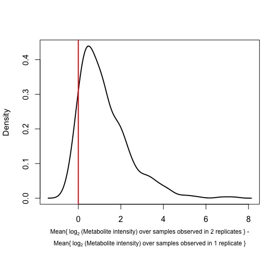
Metabolomics is the study of tissue- or body fluid-specific small molecule metabolites, and has the potential to lead to new insights into the origin of human disease [56, 15, 45] and drug metabolism [6, 13]. Recent advances in both liquid chromatography (LC) and untargeted mass spectrometry (MS) have made it possible to identify and quantify hundreds to thousands of metabolites per sample [37]. Similar to high throughput gene expression, proteomic and DNA methylation data, these data contain systematic technical and biological variation whose sources are not observed by the practitioner [46]. However, what makes untargeted LC-MS metabolomic data particularly challenging is the vast amount of missing data, nearly all of which is missing not at random due to an unknown, metabolite-specific missingness mechanism in which more abundant and ionizable analytes are more likely to be observed [12]. For instance, 22% of all #metabolites×#samples=1138×533\text{\#metabolites}\times\text{\#samples}=1138\times 533 observations were missing from our data example in Section 8, where Figure 1 shows that only analytes with the strongest signals were likely to be quantified in all technical replicates.

There are several methods that attempt to account for either latent covariates [10, 11, 46] or non-random missing data [7, 23, 39] when trying to infer the relationship between the metabolome and a variable of interest. However, these are not amenable to real, untargeted metabolomic data because the former set of methods cannot accommodate non-ignorable missing data, and the latter set ignores latent covariates that can bias estimators. Surprisingly, to the best of our knowledge, [52] is the only work to even acknowledge the challenge of accounting for both. However, they propose imputing missing data with an arbitrary limit of detection, and require prior knowledge of a set of control metabolites whose concentrations are unrelated to the variable of interest to estimate latent factors.

Given the paucity of methods to analyze untargeted metabolomic data, we developed MetabMiss, the first method to account for both latent covariates and non-random missing data that does not rely on control metabolites, internal standards or erringly imputing missing data. Our method also offers the following advantages:

  1. (a)

    We do not require knowledge of the underlying probability distribution of the missing data.

  2. (b)

    We modularize our method so that the metabolite-dependent missingness mechanisms are estimated only once per dataset, which makes computation on the order of a phenome wide association study tractable.

And while we assume the functional form of the missing data mechanism is known, we provide a method to access the veracity of said function for each metabolite.

As far as we are aware, our estimators for the missingness mechanism are also the first estimators, among those designed for mass spectrometry data, that satisfy Property (b) and do not depend on the covariate(s) of interest. This makes analyzing modern metabolomic data tractable, as practitioners are often interested in understanding the relationship between metabolite concentration and many different covariates of interest due to the wealth of information available for each for sample. We discuss this further in Section 3.1.

The remainder of the manuscript is organized as follows: we give a mathematical description of the data in Section 2 and give an overview of our method in Section 3. We describe how we estimate the metabolite-dependent missingness mechanisms, estimate the coefficients of interest in a linear model and recover latent factors in Sections 4, 5 and 6. We conclude by illustrating how our method performs in simulated and real metabolomic data in Sections 7 and 8. An R package that implements MetabMiss can be installed from github.com/chrismckennan/MetabMiss.
Refer to caption
Fig 1: A density plot of the differences in mean observed metabolite log2\log_{2}-intensity between samples with observations in both technical replicates and those from samples with only 1 observation among the two replicates. Replicate pairs were obtained by running 20 biological samples from our motivating data example twice on the same mass spectrometer.

2 Notation and problem set-up

2.1 Notation

Let n>0n>0 be an integer. We let 𝟏n,𝟎n∈ℝn\bm{1}_{n},\bm{0}_{n}\in\mathbb{R}^{n} be the vectors of all ones and zeros, In∈ℝn×nI_{n}\in\mathbb{R}^{n\times n} to be the identity matrix, [n]={1,…,n}[n]=\left\{1,\ldots,n\right\} and 𝒙i\bm{x}_{i} to be the iith element of 𝒙∈ℝn\bm{x}\in\mathbb{R}^{n}. For 𝑴∈ℝn×m\bm{M}\in\mathbb{R}^{n\times m}, we let 𝑴i​j\bm{M}_{ij} be the (i,j)(i,j)th element of 𝑴\bm{M}, and define PMP_{M} and PM⟂P_{M}^{\perp} to be the orthogonal projection matrices onto Im⁡(𝑴)={𝑴​𝒗:𝒗∈ℝm}\im\left(\bm{M}\right)=\left\{\bm{M}\bm{v}:\bm{v}\in\mathbb{R}^{m}\right\} and the null space of 𝑴T\bm{M}^{{\mathrm{\scriptscriptstyle T}}}. We also let 𝑿​∼⋅(𝝁,𝐆)\bm{X}\asim\left(\bm{\mu},\bm{G}\right) if 𝔼⁡(𝐗)=𝝁\E\left(\bm{X}\right)=\bm{\mu} and 𝕍⁡(𝐗)=𝐆\V\left(\bm{X}\right)=\bm{G}, 𝑿∼M​Nm×n​(𝝁,𝑽,𝑼)\bm{X}\sim MN_{m\times n}\left(\bm{\mu},\bm{V},\bm{U}\right) if 𝑿∈ℝm×n\bm{X}\in\mathbb{R}^{m\times n} and vec⁡(𝑿)∼Nm​n​(vec⁡(𝝁),𝑼⊗𝑽)\vecM\left(\bm{X}\right)\sim N_{mn}\left(\vecM\left(\bm{\mu}\right),\bm{U}\otimes\bm{V}\right) and lastly define Fν​(x)F_{\nu}(x) to be the cumulative distribution function of the t-distribution with ν>0\nu>0 degrees of freedom.

2.2 A description of and model for the data

Let yg​iy_{gi} be the observed or unobserved log-transformed metabolite integrated intensity for metabolite g∈[p]g\in[p] in sample i∈[n]i\in[n], where the mass spectrometer intensity, integrated over time and mass-to-charge ratio, is proportional to a metabolite’s concentration [28]. Let 𝑿=(𝒙1⋯𝒙n)T∈ℝn×d\bm{X}=\left(\bm{x}_{1}\cdots\bm{x}_{n}\right)^{{\mathrm{\scriptscriptstyle T}}}\in\mathbb{R}^{n\times d} and 𝑪=(𝒄1⋯𝒄n)T∈ℝn×K\bm{C}=\left(\bm{c}_{1}\cdots\bm{c}_{n}\right)^{{\mathrm{\scriptscriptstyle T}}}\in\mathbb{R}^{n\times K} be observed and unobserved covariates (i.e. latent factors), where the former may contain biological factors like disease status, as well as technical factors like observed batch variables. We assume

yg​i=𝒙iT​𝜷g+𝒄iT​ℓg+eg​i,eg​i​∼⋅(0,σg2),g∈[p];i∈[n],\displaystyle y_{gi}=\bm{x}_{i}^{{\mathrm{\scriptscriptstyle T}}}\bm{\beta}_{g}+\bm{c}_{i}^{{\mathrm{\scriptscriptstyle T}}}\bm{\ell}_{g}+e_{gi},\quad e_{gi}\asim\left(0,\sigma_{g}^{2}\right),\quad g\in[p];i\in[n], (2.1)

where our goal is to estimate 𝜷g\bm{\beta}_{g}. We assume the residuals {eg​i}g∈[p],i∈[n]\left\{e_{gi}\right\}_{g\in[p],i\in[n]} are independent and {eg​i}i∈[n]\left\{e_{gi}\right\}_{i\in[n]} are identically distributed for each g∈[p]g\in[p]. The unobserved covariates 𝒄i\bm{c}_{i} can confound the relationship between 𝒙i\bm{x}_{i} and yg​iy_{gi}, and also induce dependencies between different metabolites. We assume that 𝒄1,…,𝒄n\bm{c}_{1},\ldots,\bm{c}_{n} are independent and are independent of {eg​i}g∈[p],i∈[n]\left\{e_{gi}\right\}_{g\in[p],i\in[n]}. We do not assume an explicit probability model for yg​iy_{gi} in order to avoid assuming a distribution for the missing data.

We next define the indicator variable rg​i=I⁡(yg​i is observed)r_{gi}=I\left(\text{$y_{gi}$ is observed}\right) and assume that for some known increasing cumulative distribution function Ψ⁡(x)\Psi(x),

ℙ⁡(rgi=1∣ygi)=Ψ⁡{αg​(ygi−δg)},g∈[p];i∈[n].\displaystyle\Prob\left(r_{gi}=1\mid y_{gi}\right)=\Psi\left\{\alpha_{g}\left(y_{gi}-\delta_{g}\right)\right\},\quad g\in[p];i\in[n]. (2.2)

The metabolite-dependent scale and location parameters αg>0\alpha_{g}>0 and δg∈ℝ\delta_{g}\in\mathbb{R} are such that αg↘0\alpha_{g}\searrow 0 implies the mechanism is missing completely at random (MCAR) and αg↗∞\alpha_{g}\nearrow\infty implies yg​iy_{gi} is left-censored at δg\delta_{g}. Model (2.2) is consistent with Figure 1 and previous observations that metabolites with smaller intensities are less likely to be observed [12, 28], and is a classic model for missing data in untargeted mass spectrometry experiments [7, 39, 23]. Typical values for Ψ\Psi include the logistic function, an exponential probabilistic model [7, 23] and the probit function [39]. However, we observed in simulations that Ψ​(x)=F4​(x)\Psi(x)=F_{4}(x) is a more robust option, since its heavy tails make it less sensitive to outliers. This has previously been used as a robust alternative to logistic and probit functions [27].

Implicit in (2.2) is the assumption that conditional on 𝒀=(yg​i)g∈[p],i∈[n]∈ℝp×n\bm{Y}=\left(y_{gi}\right)_{g\in[p],i\in[n]}\in\mathbb{R}^{p\times n}, {rg​i}g∈[p],i∈[n]\left\{r_{gi}\right\}_{g\in[p],i\in[n]} are independent. This is likely only approximately true, since other intense analytes can preclude MS/MS fragmentation in data dependent mass spectrometry experiments. However, properly tuning the dynamic exclusion time can substantially mitigate any dependence [25].

3 A road map of our methodology

Here we provide a compendious description of our method to estimate the metabolite-dependent missingness mechanisms, recover 𝑪\bm{C} and estimate 𝜷1,…,𝜷p\bm{\beta}_{1},\ldots,\bm{\beta}_{p}. We delineate these steps in more detail in Sections 4, 5 and 6.

3.1 IV-GMM to estimate αg\alpha_{g} and δg\delta_{g}

We first estimate αg\alpha_{g} and δg\delta_{g} for metabolites gg with missing data. Unlike existing methods designed for untargeted mass spectrometry data whose estimates for the missingness mechanism depend on the user-specified 𝑿\bm{X} [7, 39, 23], our estimates only depend on 𝒀\bm{Y}, and therefore only need to be estimated once per data matrix 𝒀\bm{Y}. This makes analyzing modern datasets tractable, as practitioners typically collect a wealth of covariate information for each sample ii, and will therefore need to infer the relationship between 𝒀\bm{Y} and 𝑿\bm{X} for many different covariate matrices 𝑿\bm{X}.

Since the probability model for 𝒀\bm{Y} is unknown, we build upon [51] and use instrumental variable generalized method of moments (IV-GMM) to estimate αg\alpha_{g} and δg\delta_{g}. Fix a g∈[p]g\in[p] and let 𝑨1,…,𝑨n∈ℝs\bm{A}_{1},\ldots,\bm{A}_{n}\in\mathbb{R}^{s} be random vectors such that rg​i⊧𝑨i|yg​ir_{gi}\rotatebox[origin]{90.0}{$\models$}\bm{A}_{i}\mid y_{gi} for all i∈[n]i\in[n]. Then [51] considers the following observable s+1s+1 dimensional function for metabolite gg:

𝒉⁡{(yg​i,rg​i,𝑨i),(α,δ)}=(1​𝑨iT)T​(1−rg​i​[Ψ⁡{α⁡(yg​i−δ)}]−1),i∈[n]\displaystyle\bm{h}\left\{\left(y_{gi},r_{gi},\bm{A}_{i}\right),\left(\alpha,\delta\right)\right\}=\left(1\,\bm{A}_{i}^{{\mathrm{\scriptscriptstyle T}}}\right)^{{\mathrm{\scriptscriptstyle T}}}\left(1-r_{gi}\left[\Psi\left\{\alpha\left(y_{gi}-\delta\right)\right\}\right]^{-1}\right),\quad i\in[n] (3.1)
𝔼⁡[𝐡⁡{(ygi,rgi,𝐀i),(αg,δg)}]=𝟎s+1,i∈[n],\displaystyle\E\left[\bm{h}\left\{\left(y_{gi},r_{gi},\bm{A}_{i}\right),\left(\alpha_{g},\delta_{g}\right)\right\}\right]=\bm{0}_{s+1},\quad i\in[n],

where the second line follows from (2.2). The resulting generalized method of moments estimator for αg\alpha_{g} and δg\delta_{g} using (3.1) also requires the distribution of yg​iy_{gi} to depend on 𝑨i\bm{A}_{i} [51]. That is, 𝑨i\bm{A}_{i} must be an instrumental variable for rg​ir_{gi}.

Unfortunately, as is the case with nearly all biological data, 𝒀\bm{Y} is typically only weakly dependent on the observed covariates 𝑿\bm{X}, meaning viable instruments 𝑨i\bm{A}_{i} are almost never observed in metabolomic data. Instead, we leverage the fact that the majority of the variation in high throughput metabolomic data, like nearly all high throughput biological data, can be be explained by a relatively small number of potentially latent factors [33, 11, 42]. For example, applying principal components analysis to the metabolites with complete data from our motivating data example revealed that only 10 components were necessary to explain nearly 50% of the variation in those fully observed data. This fact forms the basis of our method to estimate each metabolite’s missingness mechanism, which we briefly describe in Algorithm 3.1.

Algorithm 3.1.

Fix ϵmiss∈[0,1)\epsilon_{\miss}\in[0,1), Kmiss≥2K_{\miss}\geq 2 and let 𝒮={g∈[p]:n−1​∑i=1n(1−rgi)≤ϵmiss}\Observed=\{g\in[p]:n^{-1}\sum\limits_{i=1}^{n}\left(1-r_{gi}\right)\leq\epsilon_{\miss}\} and ℳ={g∈[p]:n−1​∑i=1n(1−rgi)>ϵmiss}\Missing=\{g\in[p]:n^{-1}\sum\limits_{i=1}^{n}\left(1-r_{gi}\right)>\epsilon_{\miss}\} be the metabolites with (nearly) complete and missing data, respectively.

  1. (1)

    Use 𝒀𝒮=(yg​i)g∈𝒮,i∈[n]\bm{Y}_{\Observed}=\left(y_{gi}\right)_{g\in\Observed,i\in[n]} to generate KmissK_{\miss} nn-dimensional factors that explain most of the variation 𝒀𝒮\bm{Y}_{\Observed}.

  2. (2)

    For each g∈ℳg\in\Missing, select two out of the KmissK_{\miss} factors estimated in Step (1) to act as instruments for the missingness indicators rg​1,…,rg​nr_{g1},\ldots,r_{gn}.

  3. (3)

    For each g∈ℳg\in\Missing, use IV-GMM with (3.1) and instruments obtained from Step (2) to compute estimates for αg\alpha_{g} and δg\delta_{g}, α^g(GMM)\hat{\alpha}_{g}^{\GMM} and δ^g(GMM)\hat{\delta}_{g}^{\GMM}.

  4. (4)

    Identify metabolites g∈ℳg\in\Missing whose missing data patterns may not follow Model (2.2) using α^g(GMM),δ^g(GMM)\hat{\alpha}_{g}^{\GMM},\hat{\delta}_{g}^{\GMM} and the Sargan-Hansen JJ statistic.

  5. (5)

    Obtain estimates for αg,δg\alpha_{g},\delta_{g} and the weights wg​i=rg​i/Ψ⁡{αg​(yg​i−δg)}w_{gi}=r_{gi}/\Psi\left\{\alpha_{g}\left(y_{gi}-\delta_{g}\right)\right\} for g∈ℳg\in\Missing and i∈[n]i\in[n] using Hierarchical Bayesian Generalized Method of Moments (HB-GMM).

We set ϵmiss=0.05\epsilon_{\miss}=0.05 in practice because simulations show that trace amounts of missing data have negligible effects on the bias in our downstream estimators for 𝜷g\bm{\beta}_{g}. We explain how we choose KmissK_{\miss} in Section 4.2. Algorithm 3.1 tends to perform well because the estimated factors from Step (1) will be approximately the columns of (𝑿​𝑪)\left(\bm{X}\,\bm{C}\right) from Model (2.1) that explain much of the variance in 𝒀\bm{Y}. And since they are not estimated using metabolites with missing data, they will be approximately independent of rg​1,…,rg​nr_{g1},\ldots,r_{gn} conditional on yg​1,…,yg​ny_{g1},\ldots,y_{gn}, and therefore auspicious instruments for rg​1,…,rg​nr_{g1},\ldots,r_{gn} for g∈ℳg\in\Missing. We detail and provide concise, intuitive explanations of Steps (1) - (5) in Sections 4.1 - 4.5 below. We also justify Algorithm 3.1 in Sections S6 - S8 of the Supplement, where we study the asymptotic properties of the estimators from in each step when ϵmiss=0\epsilon_{\miss}=0 and n,p→∞n,p\to\infty.

3.2 Recovering latent factors and estimating coefficients of interest

Our strategy is to use the estimates from Algorithm 3.1 to first obtain 𝑪^\hat{\bm{C}}, an estimate for 𝑪\bm{C}, and then plug-in 𝑪^\hat{\bm{C}} for 𝑪\bm{C} when estimating 𝜷1,…,𝜷p\bm{\beta}_{1},\ldots,\bm{\beta}_{p}. An important feature of our method is once we run Algorithm 3.1, computing 𝑪^\hat{\bm{C}} and our software’s default estimates for 𝜷1,…,𝜷p\bm{\beta}_{1},\ldots,\bm{\beta}_{p} is fast, which makes analyzing the relationship between 𝒀\bm{Y} and tens, or even hundreds of different 𝑿\bm{X}’s computationally tractable.

4 Estimating the missingness mechanisms using Algorithm 3.1

4.1 Estimating the instruments in Step (1)

We define the factors from Step (1) of Algorithm 3.1 to be 𝑪^miss∈ℝn×Kmiss\hat{\bm{C}}_{\miss}\in\mathbb{R}^{n\times K_{\miss}}, where 𝑪^miss\hat{\bm{C}}_{\miss} is the maximum likelihood estimator for 𝑪~∈ℝn×Kmiss\tilde{\bm{C}}\in\mathbb{R}^{n\times K_{\miss}} in the model

𝒀𝒮∼M​Nps×n​(𝝁~​𝟏nT+𝑳~​𝑪~,σ~2​Ips,In),\displaystyle\bm{Y}_{\Observed}\sim MN_{p_{s}\times n}\left(\tilde{\bm{\mu}}\bm{1}_{n}^{{\mathrm{\scriptscriptstyle T}}}+\tilde{\bm{L}}\tilde{\bm{C}},\tilde{\sigma}^{2}I_{p_{s}},I_{n}\right), (4.1)

where ps=|𝒮|p_{s}=\left\lvert\Observed\right\rvert, 𝑪~T​𝟏n=𝟎Kmiss\tilde{\bm{C}}^{{\mathrm{\scriptscriptstyle T}}}\bm{1}_{n}=\bm{0}_{K_{\miss}}, n−1​𝑪~T​𝑪~=IKmissn^{-1}\tilde{\bm{C}}^{{\mathrm{\scriptscriptstyle T}}}\tilde{\bm{C}}=I_{K_{\miss}}, 𝑳~T​𝑳~\tilde{\bm{L}}^{{\mathrm{\scriptscriptstyle T}}}\tilde{\bm{L}} is diagonal with non-increasing elements and any missing data are MCAR. If ϵmiss=0\epsilon_{\miss}=0, 𝑪^miss\hat{\bm{C}}_{\miss} is a scalar multiple of the first KmissK_{\miss} right singular vectors of 𝒀𝒮​P1n⟂\bm{Y}_{\Observed}P_{1_{n}}^{\perp}. When ϵmiss>0\epsilon_{\miss}>0, the columns of 𝑪^miss\hat{\bm{C}}_{\miss} are still ordered by decreasing average effect on the log-intensities of metabolites with nearly complete data. Further, by McDiarmid’s Inequality, ℙ⁡(g∈𝒮)≤e−2​η2​n\Prob\left(g\in\Observed\right)\leq e^{-2\eta^{2}n} if n−1​∑i=1n𝔼⁡(1−rgi)≥ϵmiss+ηn^{-1}\sum\limits_{i=1}^{n}\E\left(1-r_{gi}\right)\geq\epsilon_{\miss}+\eta for η>0\eta>0, meaning it suffices to assume 𝑪^miss⊧rg​i|yg​i\hat{\bm{C}}_{\miss}\rotatebox[origin]{90.0}{$\models$}r_{gi}\mid y_{gi} if g∈ℳg\in\Missing for sufficiently large nn. That is, for 𝒉\bm{h} defined in (3.1) and 𝒄^i\hat{\bm{c}}_{i} the iith row of 𝑪^miss\hat{\bm{C}}_{\miss}, we assume 𝔼⁡[𝐡⁡{(ygi,rgi,𝐜^i),(αg,δg)}]=𝟎(Kmiss+1)\E\left[\bm{h}\left\{\left(y_{gi},r_{gi},\hat{\bm{c}}_{i}\right),\left(\alpha_{g},\delta_{g}\right)\right\}\right]=\bm{0}_{\left(K_{\miss}+1\right)} for g∈ℳg\in\Missing and i∈[n]i\in[n].

The columns of 𝑪^miss\hat{\bm{C}}_{\miss} are the factors that explain the most variation in 𝒀𝒮\bm{Y}_{\Observed}. While we expect most of them to derive from 𝑪\bm{C}, some may be related to 𝑿\bm{X} if {𝜷g}g∈𝒮\left\{\bm{\beta}_{g}\right\}_{g\in\Observed} are large enough. Note that 𝑪^miss\hat{\bm{C}}_{\miss} is invariant of the choice of 𝑿\bm{X}.

4.2 Instrument selection in Step (2)

It is critical that yg​iy_{gi} be dependent on the instruments chosen in Step (2) of Algorithm 3.1. Otherwise, the moment condition in (3.1) will not identify the parameters αg\alpha_{g} and δg\delta_{g}. We therefore use Algorithm 4.2 to only select the instruments 𝑼^g∈ℝn×2\hat{\bm{U}}_{g}\in\mathbb{R}^{n\times 2} that influence metabolite gg’s intensity.

Algorithm 4.2.

Let 𝐂^miss=(𝐂^1⋯𝐂^Kmiss)\hat{\bm{C}}_{\miss}=\left(\hat{\bm{C}}_{1}\cdots\hat{\bm{C}}_{K_{\miss}}\right) and 𝐲g=(yg​i)i∈[n]\bm{y}_{g}=\left(y_{gi}\right)_{i\in[n]}.

  1. (1)

    For each g∈ℳg\in\Missing and k∈[Kmiss]k\in\left[K_{\miss}\right], use ordinary least squares (OLS) to regress 𝒚g\bm{y}_{g} onto (𝟏n​𝑪^k)∈ℝn×2\left(\bm{1}_{n}\,\hat{\bm{C}}_{k}\right)\in\mathbb{R}^{n\times 2}, where missing data are treated as MCAR. Let pg,kp_{g,k} be the OLS P value for the null hypothesis that 𝑪^k\hat{\bm{C}}_{k} is independent of 𝒚g\bm{y}_{g}.

  2. (2)

    For each k∈[Kmiss]k\in\left[K_{\miss}\right], use {pg,k}g∈ℳ\left\{p_{g,k}\right\}_{g\in\Missing} to determine the corresponding q-values {qg,k}g∈ℳ\left\{q_{g,k}\right\}_{g\in\Missing}.

  3. (3)

    For each g∈ℳg\in\Missing, let qg,g1≤⋯≤qg,gKmissq_{g,g_{1}}\leq\cdots\leq q_{g,g_{K_{\miss}}} be the KmissK_{\miss} ordered q-values. Define 𝑼^g=(𝒖^g​1⋯𝒖^g​n)T=(𝑪^g1𝑪^g2)\hat{\bm{U}}_{g}=\left(\hat{\bm{u}}_{g1}\cdots\hat{\bm{u}}_{gn}\right)^{{\mathrm{\scriptscriptstyle T}}}=\left(\hat{\bm{C}}_{g_{1}}\,\hat{\bm{C}}_{g_{2}}\right).

We justify the regression in Step (1) using Theorem S6.1 in Section S6, which states that under technical assumptions on the distributions of 𝒀𝒮\bm{Y}_{\Observed} and 𝒚g\bm{y}_{g} for g∈ℳg\in\Missing, pg,kp_{g,k} is asymptotically uniform under the null hypothesis that 𝑪^k\hat{\bm{C}}_{k} is independent of 𝒚g\bm{y}_{g}. We also use Algorithm 4.2 to choose KmissK_{\miss}. If f⁡(k)f\left(k\right) is the fraction of metabolites g∈ℳg\in\Missing such that qg,g2≤0.05q_{g,g_{2}}\leq 0.05 assuming Kmiss=kK_{\miss}=k, we set Kmiss=min⁡{k∈{2,…,KP​A}:f⁡(k)≥0.9}K_{\miss}=\min\left\{k\in\left\{2,\ldots,K_{PA}\right\}:f\left(k\right)\geq 0.9\right\}, where KP​AK_{PA} is parallel analysis’ [5] estimate for KK under Model (4.1) with ϵmiss=0\epsilon_{\miss}=0. The estimate KmissK_{\miss} is typically much smaller than KP​AK_{PA} in practice. For example, Kmiss=10K_{\miss}=10 and KP​A=20K_{PA}=20 in our motivating data example. We show that our results are robust to the choice of KmissK_{\miss} in Section 7.

Evidently, this selection step implies 𝒖^g​i\hat{\bm{u}}_{gi} is not strictly independent of rg​ir_{gi} conditional on yg​iy_{gi}. However, we show in Section S6 of the Supplement that this dependence is asymptotically negligible under weak assumptions. We therefore assume that the indices g1,g2g_{1},g_{2} are known and 𝒖^g​i⟂⟂rg​i|yg​i\hat{\bm{u}}_{gi}\perp\mkern-9.5mu\perp r_{gi}\mid y_{gi} for the remainder of Section 4.

4.3 IV-GMM in Step (3)

Fix a g∈ℳg\in\Missing and define

𝒉g​i​(α~,δ~)=𝒉⁡{(yg​i,rg​i,𝒖^g​i),(α~,δ~)}∈ℝ3,𝒉¯g​(α~,δ~)=n−1​∑i=1n𝒉g​i​(α~,δ~).\displaystyle\bm{h}_{gi}\left(\tilde{\alpha},\tilde{\delta}\right)=\bm{h}\left\{\left(y_{gi},r_{gi},\hat{\bm{u}}_{gi}\right),\left(\tilde{\alpha},\tilde{\delta}\right)\right\}\in\mathbb{R}^{3},\quad\bar{\bm{h}}_{g}\left(\tilde{\alpha},\tilde{\delta}\right)=n^{-1}\sum\limits_{i=1}^{n}\bm{h}_{gi}\left(\tilde{\alpha},\tilde{\delta}\right). (4.2)

We let α^g(GMM)\hat{\alpha}_{g}^{\GMM} and δ^g(GMM)\hat{\delta}_{g}^{\GMM} be the two-step generalized method of moments estimators, defined as

{α^g(GMM),δ^g(GMM)}=arg​minα~>0,δ~∈ℝ⁡{𝐡¯g​(α~,δ~)T​𝐖g​𝐡¯g​(α~,δ~)},\displaystyle\left\{\hat{\alpha}_{g}^{\GMM},\hat{\delta}_{g}^{\GMM}\right\}=\argmin_{\tilde{\alpha}>0,\tilde{\delta}\in\mathbb{R}}\left\{\bar{\bm{h}}_{g}\left(\tilde{\alpha},\tilde{\delta}\right)^{{\mathrm{\scriptscriptstyle T}}}\bm{W}_{g}\bar{\bm{h}}_{g}\left(\tilde{\alpha},\tilde{\delta}\right)\right\}, (4.3)

where for {α^g(1),δ^g(1)}=arg​minα~>0,δ~∈ℝ⁡{𝒉¯g​(α~,δ~)T​𝒉¯g​(α~,δ~)}\left\{\hat{\alpha}_{g}^{(1)},\hat{\delta}_{g}^{(1)}\right\}=\mathop{\argmin}\limits_{\tilde{\alpha}>0,\tilde{\delta}\in\mathbb{R}}\left\{\bar{\bm{h}}_{g}\left(\tilde{\alpha},\tilde{\delta}\right)^{{\mathrm{\scriptscriptstyle T}}}\bar{\bm{h}}_{g}\left(\tilde{\alpha},\tilde{\delta}\right)\right\}, the weight matrix 𝑾g\bm{W}_{g} is

𝑾g=𝑾g​{α^g(1),δ^g(1)}=[n−1​∑i=1n𝒉g​i​{α^(1),δ^(1)}​𝒉g​i​{α^(1),δ^(1)}T]−1.\displaystyle\bm{W}_{g}=\bm{W}_{g}\left\{\hat{\alpha}_{g}^{(1)},\hat{\delta}_{g}^{(1)}\right\}=\left[n^{-1}\sum\limits_{i=1}^{n}\bm{h}_{gi}\left\{\hat{\alpha}^{(1)},\hat{\delta}^{(1)}\right\}\bm{h}_{gi}\left\{\hat{\alpha}^{(1)},\hat{\delta}^{(1)}\right\}^{{\mathrm{\scriptscriptstyle T}}}\right]^{-1}. (4.4)

The properties of this estimator when 𝑼^g\hat{\bm{U}}_{g} is observed and not estimated and the triplets {(rg​i,yg​i,𝒖^g​i)}i∈[n]\left\{\left(r_{gi},y_{gi},\hat{\bm{u}}_{gi}\right)\right\}_{i\in[n]} are independent are well understood [22, 51]. We extend these results in Theorem S8.1 in the Supplement to account for the uncertainty in 𝑼^g\hat{\bm{U}}_{g} and prove that under similar regularity conditions as those considered in [51], |α^g(GMM)−αg|,|δ^g(GMM)−δg|=OP(n−1/2)\left\lvert\hat{\alpha}_{g}^{\GMM}-\alpha_{g}\right\rvert,\left\lvert\hat{\delta}_{g}^{\GMM}-\delta_{g}\right\rvert=O_{P}\left(n^{-1/2}\right) and for 𝚪g​(α~,δ~)=∇α~,δ~𝒉¯g​(α~,δ~)∈ℝ3×2\bm{\Gamma}_{g}\left(\tilde{\alpha},\tilde{\delta}\right)=\nabla_{\tilde{\alpha},\tilde{\delta}}\bar{\bm{h}}_{g}\left(\tilde{\alpha},\tilde{\delta}\right)\in\mathbb{R}^{3\times 2},

n1/2𝑽^g−1/2[{α^g(GMM),δ^g(GMM)}−(αg,δg)]→dN2(𝟎,I2)\displaystyle n^{1/2}\hat{\bm{V}}_{g}^{-1/2}\left[\left\{\hat{\alpha}_{g}^{\GMM},\hat{\delta}_{g}^{\GMM}\right\}-\left(\alpha_{g},\delta_{g}\right)\right]\tdist N_{2}\left(\bm{0},I_{2}\right) (4.5a)
𝑽^g=[𝚪g​{α^g(GMM),δ^g(GMM)}T​𝑾g​𝚪g​{α^g(GMM),δ^g(GMM)}]−1\displaystyle\hat{\bm{V}}_{g}=\left[\bm{\Gamma}_{g}\left\{\hat{\alpha}_{g}^{\GMM},\hat{\delta}_{g}^{\GMM}\right\}^{{\mathrm{\scriptscriptstyle T}}}\bm{W}_{g}\bm{\Gamma}_{g}\left\{\hat{\alpha}_{g}^{\GMM},\hat{\delta}_{g}^{\GMM}\right\}\right]^{-1} (4.5b)

as n,p→∞n,p\to\infty. This result is analogous to Theorem 2 in [51], and we use this asymptotic distribution in Section 4.5 to refine our estimates for αg\alpha_{g} and δg\delta_{g}.

4.4 The Sargan-Hansen JJ statistic in Step (4)

The accuracy of downstream estimates for 𝜷g\bm{\beta}_{g} is contingent on the missing data model being approximately correct. Therefore, we leverage the fact that we use three moment conditions to estimate two parameters and use the Sargan-Hansen JJ statistic, which is routinely used to test moment restrictions in generalized method of moment estimators [22, 2, 9], to flag metabolites whose missingness mechanisms may not follow Model (2.2).

A consequence of (4.5) is that under the null hypothesis H0,gH_{0,g} that Model (2.2) is correct for metabolite g∈ℳg\in\Missing and the assumptions necessary to prove (4.5) hold, the statistic Jg=n​𝒉¯g​{α^g(GMM),δ^g(GMM)}T​𝑾g​𝒉¯g​{α^g(GMM),δ^g(GMM)}J_{g}=n\bar{\bm{h}}_{g}\left\{\hat{\alpha}_{g}^{\GMM},\hat{\delta}_{g}^{\GMM}\right\}^{{\mathrm{\scriptscriptstyle T}}}\bm{W}_{g}\bar{\bm{h}}_{g}\left\{\hat{\alpha}_{g}^{\GMM},\hat{\delta}_{g}^{\GMM}\right\} is asymptotically χ12\chi^{2}_{1} as n,p→∞n,p\to\infty, which is analogous to Lemma 4.2 in [22]. One could then use JgJ_{g} to test H0,gH_{0,g}. However, it has been repeatedly observed that using said asymptotic distribution to do inference with JgJ_{g} is anti-conservative in data with moderate, and even large sample sizes [20, 21, 4]. To circumvent this, we follow [4] and develop an empirical likelihood-derived bootstrap null distribution for JgJ_{g}, and subsequently estimate l​f​d​rg=ℙ⁡(H0,g∣Jg)lfdr_{g}=\Prob\left(H_{0,g}\mid J_{g}\right) using [48]. We then flag any metabolites with an l​f​d​rglfdr_{g} smaller than a user-specified value, which defaults to 0.8 in our software. Section S2 in the Supplement describes the details of the bootstrap procedure.

4.5 HB-GMM in Step (5)

So far we have estimated each metabolite-specific missingness mechanism independently for each metabolite g∈ℳg\in\Missing. While the mechanisms are almost certainly not identical, one might expect them to be relatively similar, and that one should be able to design a better estimator by pooling information across metabolites. Further, constructing an informative prior on the missingness mechanisms allows one to better explore the objective function in (4.3), which could be multimodal [16]. We therefore developed Hierarchical Bayesian Generalized Method of Moments (HB-GMM), a Bayesian method to estimate αg\alpha_{g}, δg\delta_{g} and the weights wg​i=rg​i/Ψ⁡{αg​(yg​i−δg)}w_{gi}=r_{gi}/\Psi\left\{\alpha_{g}\left(y_{gi}-\delta_{g}\right)\right\} for each g∈ℳg\in\Missing and i∈[n]i\in[n]. The weights play an important role in estimating 𝑪\bm{C} in Section 6.

Our method extends Bayesian generalized method of moments [29, 55, 35] by both incorporating estimated instruments and estimating an informative prior from the data. Define 𝒟={(ygi,rgi,𝐮^gi)}g∈ℳ,i∈[n]\Data=\left\{\left(y_{gi},r_{gi},\hat{\bm{u}}_{gi}\right)\right\}_{g\in\Missing,i\in[n]}. By Bayes’ rule and assuming {(αg,δg)}g∈ℳ\left\{\left(\alpha_{g},\delta_{g}\right)\right\}_{g\in\Missing} are independent and drawn from some prior distribution,

pr⁡[{(αg,δg)}g∈ℳ∣𝒟]∝pr⁡[𝒟∣{(αg,δg)}g∈ℳ]​∏g∈ℳpr⁡(αg,δg).\displaystyle\begin{aligned} \Bprob\left[\left\{\left(\alpha_{g},\delta_{g}\right)\right\}_{g\in\Missing}\mid\Data\right]\propto\Bprob\left[\Data\mid\left\{\left(\alpha_{g},\delta_{g}\right)\right\}_{g\in\Missing}\right]\prod\limits_{g\in\Missing}\Bprob\left(\alpha_{g},\delta_{g}\right).\end{aligned} (4.6)

However, the likelihood pr⁡[𝒟∣{(αg,δg)}g∈ℳ]\Bprob\left[\Data\mid\left\{\left(\alpha_{g},\delta_{g}\right)\right\}_{g\in\Missing}\right] is unknown because the distribution of yg​iy_{gi} is unknown. Nevertheless, we do know that under Model (2.2) and assuming 𝒖^g​i⟂⟂rg​i|yg​i\hat{\bm{u}}_{gi}\perp\mkern-9.5mu\perp r_{gi}\mid y_{gi} for all g∈ℳg\in\Missing and i∈[n]i\in[n], 𝒉¯g​(αg,δg)\bar{\bm{h}}_{g}\left(\alpha_{g},\delta_{g}\right) and 𝒉¯s​(αs,δs)\bar{\bm{h}}_{s}\left(\alpha_{s},\delta_{s}\right) are uncorrelated for g≠s∈ℳg\neq s\in\Missing. Further, since 𝒉¯g​(αg,δg)\bar{\bm{h}}_{g}\left(\alpha_{g},\delta_{g}\right) is an average of nn approximately independent random variables, 𝒉¯g​(αg,δg)\bar{\bm{h}}_{g}\left(\alpha_{g},\delta_{g}\right) is asymptotically normal with mean zero and variance given by (4.7) under the same assumptions used to prove (4.5).

n1/2{𝚺^g(αg,δg)}−1/2𝒉¯g(αg,δg)→dN3(𝟎3,I3) as n,p→∞,g∈ℳ𝚺^g​(αg,δg)=n−1​∑i=1n{𝒉g​i​(αg,δg)−𝒉¯g​(αg,δg)}​{𝒉g​i​(αg,δg)−𝒉¯g​(αg,δg)}T\displaystyle\begin{aligned} &n^{1/2}\left\{\hat{\bm{\Sigma}}_{g}\left(\alpha_{g},\delta_{g}\right)\right\}^{-1/2}\bar{\bm{h}}_{g}\left(\alpha_{g},\delta_{g}\right)\tdist N_{3}\left(\bm{0}_{3},I_{3}\right)\text{ as $n,p\to\infty$},\quad g\in\Missing\\ &\hat{\bm{\Sigma}}_{g}\left(\alpha_{g},\delta_{g}\right)=n^{-1}\sum\limits_{i=1}^{n}\left\{\bm{h}_{gi}\left(\alpha_{g},\delta_{g}\right)-\bar{\bm{h}}_{g}\left(\alpha_{g},\delta_{g}\right)\right\}\left\{\bm{h}_{gi}\left(\alpha_{g},\delta_{g}\right)-\bar{\bm{h}}_{g}\left(\alpha_{g},\delta_{g}\right)\right\}^{{\mathrm{\scriptscriptstyle T}}}\end{aligned} (4.7)

These facts help justify replacing the likelihood in (4.6) with the pseudo-likelihood

q[𝒟∣{(αg,δg)}g∈ℳ]=∏g∈ℳ𝒩{𝐡¯g(αg,δg)∣𝟎3,n−1𝚺^g(αg,δg)},\displaystyle q\left[\Data\mid\left\{\left(\alpha_{g},\delta_{g}\right)\right\}_{g\in\Missing}\right]=\prod\limits_{g\in\Missing}\normal\left\{\bar{\bm{h}}_{g}\left(\alpha_{g},\delta_{g}\right)\mid\bm{0}_{3},n^{-1}\hat{\bm{\Sigma}}_{g}\left(\alpha_{g},\delta_{g}\right)\right\},

where 𝒩(⋅∣𝐚,𝐛)\normal\left(\cdot\mid\bm{a},\bm{b}\right) is the likelihood of a normal distribution with mean 𝒂\bm{a} and variance 𝒃\bm{b}. The form that the pseudo-likelihood takes is computationally convenient because it implies we can sample from the pseudo-posterior

q[{(αg,δg)}g∈ℳ∣𝒟]∝∏g∈ℳ[𝒩{𝐡¯g(αg,δg)∣𝟎3,n−1𝚺^g(αg,δg)}pr(αg,δg)]\displaystyle\begin{aligned} q\left[\left\{\left(\alpha_{g},\delta_{g}\right)\right\}_{g\in\Missing}\mid\Data\right]\propto\prod\limits_{g\in\Missing}\left[\normal\left\{\bar{\bm{h}}_{g}\left(\alpha_{g},\delta_{g}\right)\mid\bm{0}_{3},n^{-1}\hat{\bm{\Sigma}}_{g}\left(\alpha_{g},\delta_{g}\right)\right\}\Bprob\left(\alpha_{g},\delta_{g}\right)\right]\end{aligned}

with Markov chain Monte Carlo using |ℳ|\left\lvert\Missing\right\rvert parallel chains, which we use to obtain

α^g\displaystyle\hat{\alpha}_{g} =𝔼⁡(αg∣𝒟),δ^g=𝔼⁡(δg∣𝒟),g∈ℳ\displaystyle=\E\left(\alpha_{g}\mid\Data\right),\quad\hat{\delta}_{g}=\E\left(\delta_{g}\mid\Data\right),\quad g\in\Missing (4.8a)
w^g​i\displaystyle\hat{w}_{gi} =𝔼⁡(wgi∣𝒟)=rgi​𝔼⁡[1/Ψ⁡{αg​(ygi−δg)}∣𝒟],g∈ℳ;i∈[n]\displaystyle=\E\left(w_{gi}\mid\Data\right)=r_{gi}\E\left[1/\Psi\left\{\alpha_{g}\left(y_{gi}-\delta_{g}\right)\right\}\mid\Data\right],\quad g\in\Missing;i\in[n] (4.8b)
v^g​i\displaystyle\hat{v}_{gi} =𝔼⁡(wgi2∣𝒟)=rgi​𝔼⁡[1/Ψ​{αg​(ygi−δg)}2∣𝒟],g∈ℳ;i∈[n].\displaystyle=\E\left(w_{gi}^{2}\mid\Data\right)=r_{gi}\E\left[1/\Psi\left\{\alpha_{g}\left(y_{gi}-\delta_{g}\right)\right\}^{2}\mid\Data\right],\quad g\in\Missing;i\in[n]. (4.8c)

This technique of replacing the likelihood with the pseudo-likelihood in (4.6) is standard in Bayesian GMM when |ℳ|=1\left\lvert\Missing\right\rvert=1 and 𝑼^g\hat{\bm{U}}_{g} is observed [29, 55, 35].

It remains to specify the prior for (αg,δg)\left(\alpha_{g},\delta_{g}\right). We assume that (log⁡(αg),δg)T|(𝝁,𝑼)∼N2​(𝝁,𝑼)\left(\log\left(\alpha_{g}\right),\delta_{g}\right)^{{\mathrm{\scriptscriptstyle T}}}\mid\left(\bm{\mu},\bm{U}\right)\sim N_{2}\left(\bm{\mu},\bm{U}\right) for all g∈ℳg\in\Missing, where we log-transform αg\alpha_{g} to make in amenable to a normal prior. We first estimate 𝝁\bm{\mu} as 𝝁^=|ℳ|−1​∑g∈ℳ(log⁡{α^g(GMM)},δ^g(GMM))T\hat{\bm{\mu}}=\left\lvert\Missing\right\rvert^{-1}\sum\limits_{g\in\Missing}\left(\log\left\{\hat{\alpha}_{g}^{\GMM}\right\},\hat{\delta}_{g}^{\GMM}\right)^{{\mathrm{\scriptscriptstyle T}}}. Assuming (4.5) is approximately correct, we then use empirical Bayes and define our estimate for 𝑼\bm{U}, 𝑼^\hat{\bm{U}}, as the maximizer of the following objective over 𝑼≻𝟎\bm{U}\succ\bm{0}:

∏g∈ℳ∫\displaystyle\prod\limits_{g\in\Missing}\int 𝒩[(log{α^g(GMM)},δ^g(GMM))T∣(ηg,δg)T,𝐑^g]𝒩{(ηg,δg)T∣𝝁^,𝐔}dηgdδg,\displaystyle\normal\left[\left(\log\left\{\hat{\alpha}_{g}^{\GMM}\right\},\hat{\delta}_{g}^{\GMM}\right)^{{\mathrm{\scriptscriptstyle T}}}\mid\left(\eta_{g},\delta_{g}\right)^{{\mathrm{\scriptscriptstyle T}}},\hat{\bm{R}}_{g}\right]\normal\left\{\left(\eta_{g},\delta_{g}\right)^{{\mathrm{\scriptscriptstyle T}}}\mid\hat{\bm{\mu}},\bm{U}\right\}d\eta_{g}d\delta_{g},

where 𝑹^g=diag⁡{1/α^g(GMM),1}​𝑽^g​diag​{1/α^g(GMM),1}\hat{\bm{R}}_{g}=\diag\left\{1/\hat{\alpha}_{g}^{\GMM},1\right\}\hat{\bm{V}}_{g}\diag\left\{1/\hat{\alpha}_{g}^{\GMM},1\right\} for 𝑽^g\hat{\bm{V}}_{g} defined in (4.5). We estimate 𝑼\bm{U} using the product of marginal likelihoods because under the assumptions used to prove (4.5), the estimates (α^g(GMM),δ^g(GMM))\left(\hat{\alpha}_{g}^{\GMM},\hat{\delta}_{g}^{\GMM}\right) and (α^s(GMM),δ^s(GMM))\left(\hat{\alpha}_{s}^{\GMM},\hat{\delta}_{s}^{\GMM}\right) are asymptotically independent for g≠s∈ℳg\neq s\in\Missing. See Section S8 in the Supplement for more details.

5 Estimating coefficients when CC is known

Here we describe our method for estimating 𝜷g\bm{\beta}_{g} and ℓg\bm{\ell}_{g} in Model (2.1) when 𝑪\bm{C} is known, which is based on inverse probability weighting [36]. This methodology is used in Section 6 to recover 𝑪\bm{C}, and is also our default method to perform inference on the coefficients of interest because estimates are consistent, it obviates specifying a probability model for the missing data and computation is fast enough to perform a metabolite phenome wide association study. For notational simplicity, we rewrite Model (2.1) as

yg​i=𝒛iT​𝜼g+eg​i,eg​i​∼⋅(0,σg2),g∈[p];i∈[n]\displaystyle y_{gi}=\bm{z}_{i}^{{\mathrm{\scriptscriptstyle T}}}\bm{\eta}_{g}+e_{gi},\quad e_{gi}\asim\left(0,\sigma_{g}^{2}\right),\quad g\in[p];i\in[n]

for the remainder of Section 5. Since estimation is trivial when there is little missing data, our goal is to estimate 𝜼g\bm{\eta}_{g} for all g∈ℳg\in\Missing when 𝒁=(𝒛1⋯𝒛n)T\bm{Z}=\left(\bm{z}_{1}\cdots\bm{z}_{n}\right)^{{\mathrm{\scriptscriptstyle T}}} is observed.

5.1 Point estimates

Fix a g∈ℳg\in\Missing and for all i∈[n]i\in[n], define the score function 𝒔g​i​(𝜼)=𝒛i​(yg​i−𝒛iT​𝜼)\bm{s}_{gi}\left(\bm{\eta}\right)=\bm{z}_{i}\left(y_{gi}-\bm{z}_{i}^{{\mathrm{\scriptscriptstyle T}}}\bm{\eta}\right), γg​i=ℙ⁡(rgi=1∣𝐙)\gamma_{gi}=\Prob\left(r_{gi}=1\mid\bm{Z}\right) and the inverse probability weighted estimating equation 𝒇g​(𝜼)=∑i=1nγ^g​i​w^g​i​𝒔g​i​(𝜼)\bm{f}_{g}\left(\bm{\eta}\right)=\sum\limits_{i=1}^{n}\hat{\gamma}_{gi}\hat{w}_{gi}\bm{s}_{gi}\left(\bm{\eta}\right), where w^g​i\hat{w}_{gi} is defined in (4.8b) and γ^g​i\hat{\gamma}_{gi} is an estimate of γg​i\gamma_{gi}. If w^g​i=wg​i\hat{w}_{gi}=w_{gi} and γ^g​i=γg​i\hat{\gamma}_{gi}=\gamma_{gi} for all i∈[n]i\in[n], then

𝔼⁡{𝐟g​(𝜼g)∣𝐙}\displaystyle\E\left\{\bm{f}_{g}\left(\bm{\eta}_{g}\right)\mid\bm{Z}\right\} =∑i=1nγg​i​𝔼⁡{𝔼⁡(wgi∣ygi)​𝐬gi​(𝜼g)∣𝐙}=∑i=1nγgi​𝔼⁡{𝐬gi​(𝜼g)∣𝐙}=𝟎.\displaystyle=\sum\limits_{i=1}^{n}\gamma_{gi}\E\left\{\E\left(w_{gi}\mid y_{gi}\right)\bm{s}_{gi}\left(\bm{\eta}_{g}\right)\mid\bm{Z}\right\}=\sum\limits_{i=1}^{n}\gamma_{gi}\E\left\{\bm{s}_{gi}\left(\bm{\eta}_{g}\right)\mid\bm{Z}\right\}=\bm{0}.

The above equality can be shown to hold in the more general case when γg​i⊧𝒚g|𝒁\gamma_{gi}\rotatebox[origin]{90.0}{$\models$}\bm{y}_{g}\mid\bm{Z} for all i∈[n]i\in[n], meaning the root of 𝒇g\bm{f}_{g} will be an accurate estimate of 𝜼g\bm{\eta}_{g} if w^g​i\hat{w}_{gi} is consistent for wg​iw_{gi} and γ^g​i\hat{\gamma}_{gi} is only weakly dependent on 𝒚g\bm{y}_{g}. We include γ^g​i\hat{\gamma}_{gi} to stabilize potentially large weights w^g​i\hat{w}_{gi} and thereby reduce the variance of our estimates, since γ^g​i\hat{\gamma}_{gi} will tend to be small if w^g​i\hat{w}_{gi} is large. This method of stabilized inverse probability weighting has been successfully applied to data that are missing at random [53], and we estimate γg​i\gamma_{gi} using a logistic regression with the estimated instruments 𝑼^g\hat{\bm{U}}_{g}. We then define our estimate for 𝜼g\bm{\eta}_{g} as the root of 𝒇g\bm{f}_{g}:

𝜼^g=(𝒁T​𝑾^g​𝒁)−1​𝒁T​𝑾^g​𝒚g,𝑾^g=diag⁡(w^g​1​γ^g​1,…,w^g​n​γ^g​n).\displaystyle\hat{\bm{\eta}}_{g}=\left(\bm{Z}^{{\mathrm{\scriptscriptstyle T}}}\hat{\bm{W}}_{g}\bm{Z}\right)^{-1}\bm{Z}^{{\mathrm{\scriptscriptstyle T}}}\hat{\bm{W}}_{g}\bm{y}_{g},\quad\hat{\bm{W}}_{g}=\diag\left(\hat{w}_{g1}\hat{\gamma}_{g1},\ldots,\hat{w}_{gn}\hat{\gamma}_{gn}\right). (5.1)

Note 𝒔g​i\bm{s}_{gi} in 𝒇g\bm{f}_{g} can be redefined to be any M-estimator, like Huber’s or Tukey’s robust estimators, provided 𝔼⁡{𝐬gi​(𝜼g)∣𝐙}=𝟎\E\left\{\bm{s}_{gi}\left(\bm{\eta}_{g}\right)\mid\bm{Z}\right\}=\bm{0}.

5.2 Quantifying uncertainty

Fix a g∈ℳg\in\Missing. Here we describe our estimator for 𝕍⁡(𝜼^g)\V\left(\hat{\bm{\eta}}_{g}\right), which we use to recover 𝑪\bm{C} in Section 6 and perform inference on 𝜼g\bm{\eta}_{g}. Our estimator is a novel finite sample-corrected sandwich variance estimator that also accounts for the uncertainty in the estimated weights w^g​i\hat{w}_{gi}.

Suppose for simplicity that w^g​i=wg​i\hat{w}_{gi}=w_{gi} and γ^g​i=γg​i\hat{\gamma}_{gi}=\gamma_{gi}. Then

n1/2(𝜼g−𝜼^g)=(n−1𝒁T𝑾^g𝒁)−1(n−1/2∑i=1nγg​iwg​ieg​i𝒛i).\displaystyle n^{1/2}\left(\bm{\eta}_{g}-\hat{\bm{\eta}}_{g}\right)=\left(n^{-1}\bm{Z}^{{\mathrm{\scriptscriptstyle T}}}\hat{\bm{W}}_{g}\bm{Z}\right)^{-1}\left(n^{-1/2}\sum\limits_{i=1}^{n}\gamma_{gi}w_{gi}e_{gi}\bm{z}_{i}\right).

Since {(yg​i,rg​i)}i∈[n]\left\{\left(y_{gi},r_{gi}\right)\right\}_{i\in[n]} are mutually independent and 𝔼⁡(γgi​wgi​egi∣𝐙)=0\E\left(\gamma_{gi}w_{gi}e_{gi}\mid\bm{Z}\right)=0,

n​𝕍⁡(𝜼^g∣𝐙)≈(n−1​𝐙T​𝐖^g​𝐙)−1​(n−1​∑i=1nγgi2​wgi2​egi2​𝐳i​𝐳iT)​(n−1​𝐙T​𝐖^g​𝐙)−1.\displaystyle n\V\left(\hat{\bm{\eta}}_{g}\mid\bm{Z}\right)\approx\left(n^{-1}\bm{Z}^{{\mathrm{\scriptscriptstyle T}}}\hat{\bm{W}}_{g}\bm{Z}\right)^{-1}\left(n^{-1}\sum\limits_{i=1}^{n}\gamma_{gi}^{2}w_{gi}^{2}e_{gi}^{2}\bm{z}_{i}\bm{z}_{i}^{{\mathrm{\scriptscriptstyle T}}}\right)\left(n^{-1}\bm{Z}^{{\mathrm{\scriptscriptstyle T}}}\hat{\bm{W}}_{g}\bm{Z}\right)^{-1}.

Therefore, we need only approximate the middle term to estimate 𝕍⁡(𝜼^g∣𝐙)\V\left(\hat{\bm{\eta}}_{g}\mid\bm{Z}\right). Simply plugging in w^g​i2\hat{w}_{gi}^{2} for wg​i2w_{gi}^{2} will tend to underestimate 𝕍⁡(𝜼^g∣𝐙)\V\left(\hat{\bm{\eta}}_{g}\mid\bm{Z}\right), since the uncertainty in w^g​i\hat{w}_{gi} increases as wg​iw_{gi} increases. Further, plugging in e^g​i=yg​i−𝒛iT​𝜼^g\hat{e}_{gi}=y_{gi}-\bm{z}_{i}^{{\mathrm{\scriptscriptstyle T}}}\hat{\bm{\eta}}_{g} for eg​ie_{gi} will also underestimate 𝕍⁡(𝜼^g∣𝐙)\V\left(\hat{\bm{\eta}}_{g}\mid\bm{Z}\right), since this ignores the uncertainty in 𝜼^g\hat{\bm{\eta}}_{g}. We circumvent the former by replacing wg​i2w_{gi}^{2} with v^g​i\hat{v}_{gi} defined in (4.8c), where v^g​i≥w^g​i2\hat{v}_{gi}\geq\hat{w}_{gi}^{2} such that v^g​i=w^g​i2\hat{v}_{gi}=\hat{w}_{gi}^{2} if and only if 𝕍⁡(wgi∣𝒟)=0\V\left(w_{gi}\mid\Data\right)=0. That is, v^g​i\hat{v}_{gi} helps account for the uncertainty in our estimate for wg​iw_{gi}. We lastly show how we estimate eg​i2e_{gi}^{2} in Section S4 of the Supplement, which leads to the following estimate for 𝕍⁡(𝜼^g∣𝐙)\V\left(\hat{\bm{\eta}}_{g}\mid\bm{Z}\right):

𝕍^​(𝜼^g∣𝒁)=(𝒁T​𝑾^g​𝒁)−1​{∑i=1n(1−h^g​i)−2​γ^g​i2​v^g​i​e^g​i2​𝒛i​𝒛iT}​(𝒁T​𝑾^g​𝒁)−1.\displaystyle\hat{\V}\left(\hat{\bm{\eta}}_{g}\mid\bm{Z}\right)=\left(\bm{Z}^{{\mathrm{\scriptscriptstyle T}}}\hat{\bm{W}}_{g}\bm{Z}\right)^{-1}\left\{\sum\limits_{i=1}^{n}\left(1-\hat{h}_{gi}\right)^{-2}\hat{\gamma}_{gi}^{2}\hat{v}_{gi}\hat{e}_{gi}^{2}\bm{z}_{i}\bm{z}_{i}^{{\mathrm{\scriptscriptstyle T}}}\right\}\left(\bm{Z}^{{\mathrm{\scriptscriptstyle T}}}\hat{\bm{W}}_{g}\bm{Z}\right)^{-1}. (5.2)

The term (1−h^g​i)−2\left(1-\hat{h}_{gi}\right)^{-2} is a finite sample correction, where h^g​i\hat{h}_{gi} is the iith leverage score of 𝑾^g1/2​𝒁\hat{\bm{W}}_{g}^{1/2}\bm{Z} for i∈[n]i\in[n]. This resembles the (1−h^g​i)−1\left(1-\hat{h}_{gi}\right)^{-1} inflation term commonly used to correct the sandwich variance estimator [50]. The difference arises because the residuals eg​1,…,eg​ne_{g1},\ldots,e_{gn} are dependent on the design matrix 𝑾^g1/2​𝒁\hat{\bm{W}}_{g}^{1/2}\bm{Z} when data are missing not at random (MNAR). As far as we are aware, this is the first such finite sample variance correction for inverse probability weighted estimators with data that are MNAR.

6 Recovering CC when data are MNAR

Here we describe our method for estimating the latent covariates 𝑪\bm{C}, where we now return to using the notation of Model (2.1). Define 𝑿int\bm{X}_{\interest} and 𝑿nuis\bm{X}_{\nuisance} such that 𝑿=(𝑿int​𝑿nuis)\bm{X}=\left(\bm{X}_{\interest}\,\bm{X}_{\nuisance}\right), where 𝑿int\bm{X}_{\interest} contains the covariates of interest like disease status and 𝑿nuis\bm{X}_{\nuisance} contains observed nuisance covariates like the intercept and technical factors. We assume for simplicity of presentation that 𝑿=𝑿int\bm{X}=\bm{X}_{\interest}, and we describe the simple extension when 𝑿=(𝑿int​𝑿nuis)\bm{X}=\left(\bm{X}_{\interest}\,\bm{X}_{\nuisance}\right) in Section S3 in the Supplement.

Let 𝒚g=(yg​i)i∈[n]\bm{y}_{g}=\left(y_{gi}\right)_{i\in[n]} and 𝒆g=(eg​i)i∈[n]\bm{e}_{g}=\left(e_{gi}\right)_{i\in[n]} for each g∈[p]g\in[p]. Then

𝒚g=𝑿𝜷~g+𝑪2ℓg+𝒆g,𝜷~g=𝜷g+𝛀ℓg,𝒆g∼⋅(𝟎n,σg2In),g∈[p]\displaystyle\bm{y}_{g}=\bm{X}\tilde{\bm{\beta}}_{g}+\bm{C}_{2}\bm{\ell}_{g}+\bm{e}_{g},\quad\tilde{\bm{\beta}}_{g}=\bm{\beta}_{g}+\bm{\Omega}\bm{\ell}_{g},\quad\bm{e}_{g}\asim\left(\bm{0}_{n},\sigma_{g}^{2}I_{n}\right),\quad g\in[p] (6.1a)
𝛀=(𝑿T​𝑿)−1​𝑿T​𝑪,𝑪2=PX⟂​𝑪.\displaystyle\bm{\Omega}=\left(\bm{X}^{{\mathrm{\scriptscriptstyle T}}}\bm{X}\right)^{-1}\bm{X}^{{\mathrm{\scriptscriptstyle T}}}\bm{C},\quad\bm{C}_{2}=P_{X}^{\perp}\bm{C}. (6.1b)

It is easy to show that typical estimates for 𝜷g\bm{\beta}_{g} using the design matrices (𝑿​𝑪^)\left(\bm{X}\,\hat{\bm{C}}\right) and (𝑿​𝑪)\left(\bm{X}\,\bm{C}\right), like OLS and that in (5.1), will be identical if Im⁡(𝑪^)=Im⁡(𝑪)\im\left(\hat{\bm{C}}\right)=\im\left(\bm{C}\right). Consequently, we need only estimate Im⁡(𝑪)\im\left(\bm{C}\right), which is quite auspicious because even though 𝑪\bm{C} is not identifiable in (2.1), Im⁡(𝑪)\im\left(\bm{C}\right) is identifiable under assumptions on the sparsity of (𝜷1⋯𝜷p)\left(\bm{\beta}_{1}\cdots\bm{\beta}_{p}\right) [38]. We therefore assume without loss of generality that 𝑪\bm{C} and our estimator for 𝑪\bm{C}, 𝑪^\hat{\bm{C}}, satisfy =n−1​𝑪T​PX⟂​𝑪=n−1​𝑪^T​PX⟂​𝑪^=IK=n^{-1}\bm{C}^{{\mathrm{\scriptscriptstyle T}}}P_{X}^{\perp}\bm{C}=n^{-1}\hat{\bm{C}}^{{\mathrm{\scriptscriptstyle T}}}P_{X}^{\perp}\hat{\bm{C}}=I_{K}. We estimate 𝑪2\bm{C}_{2} and 𝛀\bm{\Omega} in Sections 6.1 and 6.2 below, and define

𝑪^=𝑿​𝛀^+𝑪^2.\displaystyle\hat{\bm{C}}=\bm{X}\hat{\bm{\Omega}}+\hat{\bm{C}}_{2}. (6.2)

For 𝒁=(𝑿​𝑪^)\bm{Z}=\left(\bm{X}\,\hat{\bm{C}}\right) and 𝑹g=diag⁡(rg​1,…,rg​n)\bm{R}_{g}=\diag\left(r_{g1},\ldots,r_{gn}\right), our estimates for 𝜼g=(𝜷gT,ℓgT)T\bm{\eta}_{g}=\left(\bm{\beta}_{g}^{{\mathrm{\scriptscriptstyle T}}},\bm{\ell}_{g}^{{\mathrm{\scriptscriptstyle T}}}\right)^{{\mathrm{\scriptscriptstyle T}}} are

𝜼^g=\displaystyle\hat{\bm{\eta}}_{g}= {(𝒁T​𝑹g​𝒁)−1​𝒁T​𝑹g​𝒚gif g∈𝒮(5.1)if g∈ℳ\displaystyle\begin{cases}\left(\bm{Z}^{{\mathrm{\scriptscriptstyle T}}}\bm{R}_{g}\bm{Z}\right)^{-1}\bm{Z}^{{\mathrm{\scriptscriptstyle T}}}\bm{R}_{g}\bm{y}_{g}&\text{if $g\in\Observed$}\\ \eqref{equation:IPW:beta.hat}&\text{if $g\in\Missing$}\end{cases} (6.3a)
𝕍^​(𝜼^g)=\displaystyle\hat{\V}\left(\hat{\bm{\eta}}_{g}\right)= {{Tr⁡(𝑹g)−d−K}−1​‖𝑹g​(𝒚g−𝒁​𝜼^g)‖22​(𝒁T​𝑹g​𝒁)−1if g∈𝒮(5.2)if g∈ℳ.\displaystyle\begin{cases}\{\Tr(\bm{R}_{g})-d-K\}^{-1}\left\lVert\bm{R}_{g}\left(\bm{y}_{g}-\bm{Z}\hat{\bm{\eta}}_{g}\right)\right\rVert_{2}^{2}\left(\bm{Z}^{{\mathrm{\scriptscriptstyle T}}}\bm{R}_{g}\bm{Z}\right)^{-1}&\text{if $g\in\Observed$}\\ \eqref{equation:IPW:Variance}&\text{if $g\in\Missing$.}\end{cases} (6.3b)

6.1 Estimating latent factors that are orthogonal to the design

We first describe our estimators for 𝜷~g\tilde{\bm{\beta}}_{g}, ℓg\bm{\ell}_{g} and 𝑪2\bm{C}_{2}, which we also use in Section 6.2 to estimate 𝛀\bm{\Omega}. Let ℳ1={g∈ℳ:lfdrg≥0.8}\Missingsub=\left\{g\in\Missing:lfdr_{g}\geq 0.8\right\} be the set of metabolites with missing data whose missingness mechanisms appear to follow (2.2), where l​f​d​rglfdr_{g} was defined in Section 4.4. We estimate 𝜷~g,ℓg\tilde{\bm{\beta}}_{g},\bm{\ell}_{g} and 𝑪2\bm{C}_{2} using metabolites with nearly complete data or missing data whose missingness mechanisms appear to follow (2.2) with the following scaled quasi-likelihood obsjective function, under the restriction that 𝑪2T​𝑿=𝟎\bm{C}_{2}^{{\mathrm{\scriptscriptstyle T}}}\bm{X}=\bm{0} and n−1​𝑪2T​𝑪2=IKn^{-1}\bm{C}_{2}^{{\mathrm{\scriptscriptstyle T}}}\bm{C}_{2}=I_{K}:

{{𝜷~^g}g∈𝒮∪ℳ1,{ℓ^g}g∈𝒮∪ℳ1,𝑪^2}=arg​max𝜷~g∈ℝd,ℓg∈ℝK𝐂2∈ℝn×K[−∑g∈𝒮‖𝐑g{𝐲g−(𝐗𝜷~g+𝐂2ℓg)}‖22−∑g∈ℳ1‖𝑾^g1/2{𝒚g−(𝑿𝜷~g+𝑪2ℓg)}‖22].\displaystyle\begin{aligned} \left\{\left\{\hat{\tilde{\bm{\beta}}}_{g}\right\}_{g\in\Observed\cup\Missingsub},\left\{\hat{\bm{\ell}}_{g}\right\}_{g\in\Observed\cup\Missingsub},\hat{\bm{C}}_{2}\right\}=&\argmax_{\begin{subarray}{c}\tilde{\bm{\beta}}_{g}\in\mathbb{R}^{d},\,\bm{\ell}_{g}\in\mathbb{R}^{K}\\ \bm{C}_{2}\in\mathbb{R}^{n\times K}\end{subarray}}\left[-\sum\limits_{g\in\Observed}\left\lVert\bm{R}_{g}\left\{\bm{y}_{g}-\left(\bm{X}\tilde{\bm{\beta}}_{g}+\bm{C}_{2}\bm{\ell}_{g}\right)\right\}\right\rVert_{2}^{2}\right.\\ &\left.-\sum\limits_{g\in\Missingsub}\left\lVert\hat{\bm{W}}_{g}^{1/2}\left\{\bm{y}_{g}-\left(\bm{X}\tilde{\bm{\beta}}_{g}+\bm{C}_{2}\bm{\ell}_{g}\right)\right\}\right\rVert_{2}^{2}\right].\end{aligned}

This optimization treats missing data from metabolites with little to no missing data as MCAR. For fixed 𝑪2\bm{C}_{2}, the updates for 𝜷~g\tilde{\bm{\beta}}_{g} and ℓg\bm{\ell}_{g} are given by (6.3a) with 𝒁=(𝑿​𝑪2)\bm{Z}=\left(\bm{X}\,\bm{C}_{2}\right).

6.2 Estimating latent factors in the image of the design

We now describe how we estimate 𝛀\bm{\Omega}. The estimates (𝜷~^gT,ℓ^gT)T\left(\hat{\tilde{\bm{\beta}}}_{g}^{{\mathrm{\scriptscriptstyle T}}},\hat{\bm{\ell}}_{g}^{{\mathrm{\scriptscriptstyle T}}}\right)^{{\mathrm{\scriptscriptstyle T}}} can be expressed as (6.3a) using the design matrix 𝒁=(𝑿​𝑪^2)\bm{Z}=\left(\bm{X}\,\hat{\bm{C}}_{2}\right). By (6.1a), this suggests an appropriate model for 𝜷~^g\hat{\tilde{\bm{\beta}}}_{g} is 𝜷~^g​∼⋅(𝜷g+𝛀​ℓg,𝕍^​(𝜷~^g))\hat{\tilde{\bm{\beta}}}_{g}\asim\left(\bm{\beta}_{g}+\bm{\Omega}\bm{\ell}_{g},\hat{\V}\left(\hat{\tilde{\bm{\beta}}}_{g}\right)\right), where 𝕍^​(𝜷~^g)∈ℝd×d\hat{\V}\left(\hat{\tilde{\bm{\beta}}}_{g}\right)\in\mathbb{R}^{d\times d} is the upper left d×dd\times d submatrix of 𝕍^​(𝜼^g)\hat{\V}\left(\hat{\bm{\eta}}_{g}\right) defined in (6.3b) for 𝒁=(𝑿​𝑪^2)\bm{Z}=\left(\bm{X}\,\hat{\bm{C}}_{2}\right). If (𝜷1⋯𝜷p)\left(\bm{\beta}_{1}\cdots\bm{\beta}_{p}\right) is sparse, the expression for 𝜷~g\tilde{\bm{\beta}}_{g} in (6.1a) suggests we can regress the estimates for 𝜷~g\tilde{\bm{\beta}}_{g} onto those for ℓg\bm{\ell}_{g} to estimate 𝛀\bm{\Omega}. This is outlined in Algorithm 6.3.

Algorithm 6.3 (Estimating 𝛀\bm{\Omega}).

Let ϵq∈[0,1]\epsilon_{\qvalue}\in[0,1], R≥0R\geq 0 be an integer and τ^g,j\hat{\tau}_{g,j} be the jjth diagonal element of 𝕍^​(𝛃~^g)∈ℝd×d\hat{\V}\left(\hat{\tilde{\bm{\beta}}}_{g}\right)\in\mathbb{R}^{d\times d} for all g∈𝒮∪ℳ1g\in\Observed\cup\Missingsub and j∈[d]j\in[d].

  1. (0)

    For j∈[d]j\in[d], let 𝛀^j(0)=(∑g∈𝒮∪ℳ1τ^g,j−1​ℓ^g​ℓ^gT)−1​(∑g∈𝒮∪ℳ1τ^g,j−1​𝜷~^gj​ℓ^g)\hat{\bm{\Omega}}^{(0)}_{j}=\left(\sum\limits_{g\in\Observed\cup\Missingsub}\hat{\tau}_{g,j}^{-1}\hat{\bm{\ell}}_{g}\hat{\bm{\ell}}_{g}^{{\mathrm{\scriptscriptstyle T}}}\right)^{-1}\left(\sum\limits_{g\in\Observed\cup\Missingsub}\hat{\tau}_{g,j}^{-1}\hat{\tilde{\bm{\beta}}}_{g_{j}}\hat{\bm{\ell}}_{g}\right) and 𝛀^(0)=(𝛀^1(0)⋯𝛀^d(0))T\hat{\bm{\Omega}}^{(0)}=\left(\hat{\bm{\Omega}}^{(0)}_{1}\cdots\hat{\bm{\Omega}}^{(0)}_{d}\right)^{{\mathrm{\scriptscriptstyle T}}}. Define 𝑪^(0)=𝑿​𝛀^(0)+𝑪^2\hat{\bm{C}}^{(0)}=\bm{X}\hat{\bm{\Omega}}^{(0)}+\hat{\bm{C}}_{2}. If R=0R=0, return 𝑪^=𝑪^(0)\hat{\bm{C}}=\hat{\bm{C}}^{(0)}.

  2. (1)

    Let 𝑪^(r)\hat{\bm{C}}^{(r)} be given. Define 𝜷^g(r)\hat{\bm{\beta}}_{g}^{(r)} and 𝕍^​{𝜷^g(r)}\hat{\V}\left\{\hat{\bm{\beta}}_{g}^{(r)}\right\} to be the first dd coordinates and upper left d×dd\times d block of 𝜼^g\hat{\bm{\eta}}_{g} and 𝕍^​(𝜼^g)\hat{\V}\left(\hat{\bm{\eta}}_{g}\right) defined in (6.3a) and (6.3b), respectively, for 𝒁=(𝑿​𝑪^(r))\bm{Z}=\left(\bm{X}\,\hat{\bm{C}}^{(r)}\right). For z2∼χ12z^{2}\sim\chi^{2}_{1}, let pg,j=ℙ[z2≥{𝜷^g(r)}2/𝕍^{𝜷^g(r)}jj]p_{g,j}=\Prob\left[z^{2}\geq\left\{\hat{\bm{\beta}}_{g}^{(r)}\right\}^{2}/\hat{\V}\left\{\hat{\bm{\beta}}_{g}^{(r)}\right\}_{jj}\right] for all g∈𝒮∪ℳ1g\in\Observed\cup\Missingsub and j∈[d]j\in[d].

  3. (2)

    Obtain the q-values {qg,j}g∈𝒮∪ℳ1\left\{q_{g,j}\right\}_{g\in\Observed\cup\Missingsub} using the P values {pg,j}g∈𝒮∪ℳ1\left\{p_{g,j}\right\}_{g\in\Observed\cup\Missingsub} for each j∈[d]j\in[d]. Define 𝛀^(r+1)=(𝛀^1(r+1)⋯𝛀^d(r+1))T\hat{\bm{\Omega}}^{(r+1)}=\left(\hat{\bm{\Omega}}^{(r+1)}_{1}\cdots\hat{\bm{\Omega}}^{(r+1)}_{d}\right)^{{\mathrm{\scriptscriptstyle T}}} to be

    𝛀^j(r+1)=\displaystyle\hat{\bm{\Omega}}^{(r+1)}_{j}= {∑g∈𝒮∪ℳ1I⁡(qg,j>ϵq)​τ^g,j−1​ℓ^g​ℓ^gT}−1​{∑g∈𝒮∪ℳ1I⁡(qg,j>ϵq)​τ^g,j−1​𝜷~^gj​ℓ^g}.\displaystyle\left\{\sum\limits_{g\in\Observed\cup\Missingsub}I\left(q_{g,j}>\epsilon_{\qvalue}\right)\hat{\tau}_{g,j}^{-1}\hat{\bm{\ell}}_{g}\hat{\bm{\ell}}_{g}^{{\mathrm{\scriptscriptstyle T}}}\right\}^{-1}\left\{\sum\limits_{g\in\Observed\cup\Missingsub}I\left(q_{g,j}>\epsilon_{\qvalue}\right)\hat{\tau}_{g,j}^{-1}\hat{\tilde{\bm{\beta}}}_{g_{j}}\hat{\bm{\ell}}_{g}\right\}.

    Update r←r+1r\leftarrow r+1 and define 𝑪^(r)=𝑿​𝛀^(r)+𝑪^2\hat{\bm{C}}^{(r)}=\bm{X}\hat{\bm{\Omega}}^{(r)}+\hat{\bm{C}}_{2}.

  4. (3)

    Repeat Steps (1) and (2) for r=0,1,…,R−1r=0,1,\ldots,R-1 and return 𝛀^=𝛀^(R)\hat{\bm{\Omega}}=\hat{\bm{\Omega}}^{(R)}.

Our software’s default is ϵq=0.1\epsilon_{\qvalue}=0.1 and R=3R=3. While 𝛀^(0)\hat{\bm{\Omega}}^{(0)} is a suitable estimate for 𝛀\bm{\Omega} when (𝜷1⋯𝜷p)\left(\bm{\beta}_{1}\cdots\bm{\beta}_{p}\right) is very sparse, Step (2) identifies and removes metabolites with non-zero coefficients of interest 𝜷g\bm{\beta}_{g} and helps alleviate the impact of outliers in the regression estimate for 𝛀\bm{\Omega} when (𝜷1⋯𝜷p)\left(\bm{\beta}_{1}\cdots\bm{\beta}_{p}\right) is only approximately sparse.

7 A simulation study

7.1 Simulation setup

Here we analyze simulated metabolomic data to compare the performance of our method with other existing methods. We simulated the log-intensities of p=1200p=1200 metabolites in n=600n=600 individuals, 300 of which were cases and the remaining 300 were controls. The observed design matrix was 𝑿=(𝑿int​ 1n)\bm{X}=\left(\bm{X}_{\interest}\,\bm{1}_{n}\right), where 𝑿int=(𝟏n/2T,𝟎n/2T)T∈ℝn\bm{X}_{\interest}=\left(\bm{1}_{n/2}^{{\mathrm{\scriptscriptstyle T}}},\bm{0}_{n/2}^{{\mathrm{\scriptscriptstyle T}}}\right)^{{\mathrm{\scriptscriptstyle T}}}\in\mathbb{R}^{n}. The parameters pp and nn were chosen to match those from our real data example in Section 8, and we include additional results when n=100n=100 and n=300n=300 in Section S5.3 of the supplement. We set K=10K=10, and for some constant aa and appropriate Ψ⁡(x)\Psi(x), simulated data as

log⁡(αg)∼N1​(μα,0.42),δg∼N1​(16,1.22),g∈[p]\displaystyle\log\left(\alpha_{g}\right)\sim N_{1}\left(\mu_{\alpha},0.4^{2}\right),\quad\delta_{g}\sim N_{1}\left(16,1.2^{2}\right),\quad g\in[p] (7.1a)
𝑪=(𝒄1⋯𝒄n)T∼MNn×K((a𝑿int 0n⋯𝟎n),In,IK)\displaystyle\bm{C}=\left(\bm{c}_{1}\cdots\bm{c}_{n}\right)^{{\mathrm{\scriptscriptstyle T}}}\sim MN_{n\times K}\left(\left(a\bm{X}_{\interest}\,\bm{0}_{n}\cdots\bm{0}_{n}\right),I_{n},I_{K}\right) (7.1b)
ℓgk∼πk​δ0+(1−πk)​N1​(0,τk2),g∈[p];k∈[K]\displaystyle\bm{\ell}_{g_{k}}\sim\pi_{k}\delta_{0}+\left(1-\pi_{k}\right)N_{1}\left(0,\tau_{k}^{2}\right),\quad g\in[p];k\in[K] (7.1c)
μg∼N1​(18,52),σg2∼Gamma​(0.2−2,0.2−2),g∈[p]\displaystyle\mu_{g}\sim N_{1}\left(18,5^{2}\right),\quad\sigma_{g}^{2}\sim\text{Gamma}\left(0.2^{-2},0.2^{-2}\right),\quad g\in[p] (7.1d)
βg∼0.8​δ0+0.2​N1​(0,0.42),g∈[p]\displaystyle\beta_{g}\sim 0.8\delta_{0}+0.2N_{1}\left(0,0.4^{2}\right),\quad g\in[p] (7.1e)
yg​i∼N1​(μg+𝑿inti​βg+𝒄iT​ℓg,σg2),g∈[p];i∈[n]\displaystyle y_{gi}\sim N_{1}\left(\mu_{g}+\bm{X}_{\interest_{i}}\beta_{g}+\bm{c}_{i}^{{\mathrm{\scriptscriptstyle T}}}\bm{\ell}_{g},\sigma_{g}^{2}\right),\quad g\in[p];i\in[n] (7.1f)
rg​i=Bernoulli​[Ψ⁡{αg​(yg​i−δg)}],g∈[p];i∈[n]\displaystyle r_{gi}=\text{Bernoulli}\left[\Psi\left\{\alpha_{g}\left(y_{gi}-\delta_{g}\right)\right\}\right],\quad g\in[p];i\in[n] (7.1g)

where δ0\delta_{0} is the point mass at 0 and μα\mu_{\alpha} in (7.1a) was set so that if ZZ has cumulative distribution function Ψ​{exp⁡(μα)​x}\Psi\left\{\exp\left(\mu_{\alpha}\right)x\right\}, 𝕍⁡(Z)=1\V(Z)=1. The constant aa in (7.1b) was chosen so that 𝑪\bm{C} explained 7.5% of the variance in 𝑿int\bm{X}_{\interest} on average across all simulations, and Table 1 contains the values of πk\pi_{k} and τk2\tau_{k}^{2}. These were chosen so that the non-zero eigenvalues λ1,…,λK\lambda_{1},\ldots,\lambda_{K} of ℐ=(n−1)−1​P1n⟂​𝑪​(p−1​∑g=1pσg−2​ℓg​ℓgT)​𝑪T​P1n⟂\mathcal{I}=(n-1)^{-1}P_{1_{n}}^{\perp}\bm{C}\left(p^{-1}\sum\limits_{g=1}^{p}\sigma_{g}^{-2}\bm{\ell}_{g}\bm{\ell}_{g}^{{\mathrm{\scriptscriptstyle T}}}\right)\bm{C}^{{\mathrm{\scriptscriptstyle T}}}P_{1_{n}}^{\perp} were 0.61, 0.33, 0.19, 0.14, 0.12, 0.08, 0.07, 0.05, 0.05 and 0.05 on average across all simulated datasets, since these were the first 10 eigenvalues of the estimated ℐ\mathcal{I} in our data example in Section 8. Similarly, the prior variances for the missingness mechanism parameters in (7.1a), as well as the mean and variance for the global mean μg\mu_{g} in (7.1d), were set to their estimated equivalents from our data example in Section 8. Since we typically do not know the exact functional form of Ψ⁡(x)\Psi(x) in practice, we set Ψ⁡(x)=exp⁡(x)/{1+exp⁡(x)}\Psi(x)=\exp(x)/\left\{1+\exp(x)\right\} and analyzed each simulated dataset assuming Ψ​(x)=F4​(x)\Psi(x)=F_{4}(x). The distribution of missing data is given in Table 2, which closely matched that in our real data example.

Table 1: The πk\pi_{k} and τk\tau_{k} values used to simulate ℓ1,…,ℓp\bm{\ell}_{1},\ldots,\bm{\ell}_{p} (k=1,…,10k=1,\ldots,10).
Factor number (kk) 11 22 33 44 55 66 77 88 99 1010
πk\pi_{k} 0 0 0.76 0.56 0.48 0.32 0.28 0.20 0.20 0.20
τk\tau_{k} 0.78 0.57 0.5 0.5 0.5 0.5 0.5 0.5 0.5 0.5
Table 2: The expected number of metabolites in each missing data bin for data simulated according to (7.1) with Ψ⁡(x)=exp⁡(x)/{1+exp⁡(x)}\Psi(x)=\exp(x)/\left\{1+\exp(x)\right\}, where ff is the frequency of missing data.
f=0f=0 0<f≤0.050<f\leq 0.05 0.05<f≤0.50.05<f\leq 0.5 0.5<f0.5<f
251.6 233.6 298.3 416.4

We simulated 60 datasets and in each simulation, removed all metabolites that were missing in more than 50% of the samples, since we find that these metabolites tend to have large JJ statistics in real data. We used Algorithm 3.1 with ϵmiss=0.05\epsilon_{\miss}=0.05 and Kmiss=5K_{\miss}=5 to estimate the metabolite-dependent missingness mechanism parameters αg\alpha_{g} and δg\delta_{g}, and subsequently estimated 𝑪\bm{C} as (6.2) with ϵq=0.1\epsilon_{\qvalue}=0.1, assuming K=10K=10 was known. We lastly estimated βg\beta_{g} and said estimator’s variance using (6.3), and formed 95% confidence intervals and computed P values assuming β^g∼N1​(βg,𝕍^​(β^g))\hat{\beta}_{g}\sim N_{1}\left(\beta_{g},\hat{\V}\left(\hat{\beta}_{g}\right)\right). We refer to this procedure as “MetabMiss”.

Similar to our real data example, KmissK_{\miss} was such that qg,g2q_{g,g_{2}}, defined in Algorithm 4.2, was less than 0.05 in at least 90% of all metabolites g∈ℳg\in\Missing in each simulated dataset. Our results were identical when we let KmissK_{\miss} be as small as 3 and as large as 10. The fact that KK was assumed to be known when estimating 𝑪\bm{C} was inconsequential, since parallel analysis [32] applied to metabolites with only complete data consistently estimated K=10K=10. We demonstrate the fidelity of MetabMiss’ estimates for the coefficients of interest β1,…,βp\beta_{1},\ldots,\beta_{p} in Section 7.2. We also illustrate the accuracy of Algorithm 3.1’s estimates for αg\alpha_{g} and δg\delta_{g}, as well as the uniformity of the bootstrapped Sargan-Hansen JJ statistic P values, in Section S5.1.

7.2 Simulation results

Given the paucity of methods available to analyze metabolomics data, we could only compare our method to those that account for non-random missing data or 𝑪\bm{C}, but not both. It is not interesting to compare MetabMiss to methods that only account for the former, like those proposed in [7, 23, 39], because ignoring 𝑪\bm{C} will dramatically inflate type I error. Instead, we compared MetabMiss to existing methods that have been used to recover 𝑪\bm{C} in metabolomic data but do not account for the non-random missing data, which included IRW-SVA [34], dSVA [31], RUV-2 [19] and RUV-4 [18]. We do not report results from the method proposed in [49], as it performed nearly identically to dSVA in all simulation scenarios. Since none of the of the aforementioned methods can accommodate missing data, we estimated 𝑪\bm{C} with each using only metabolites with complete observations, and computed confidence intervals and P values using OLS with the estimated design matrix (𝑿​𝑪^)\left(\bm{X}\,\hat{\bm{C}}\right), assuming missing data were MCAR. We remark that we could not analyze these simulated data with the methods proposed in [10] or [46] because both methods rely on a random effects model whose implemented estimators are not amenable to any missing data.

We first evaluated each method’s ability to identify metabolites with non-zero effect of interest βg\beta_{g} while controlling the false discovery rate at a nominal level. The results are given in Figure 2, where the only method to suitably control for false discoveries is MetabMiss. The fact that MetabMiss is slightly underpowered compared to the other methods is to be expected, as anti-conservative inference is typically more powerful. We also evaluated the confidence interval coverage for the effects of interest βg\beta_{g} for each method in Figure 3. These results illustrate the consequences of performing inference on estimators that do not properly account for the missing data, and also highlight the fidelity of our finite sample-corrected estimator for the variance defined in (5.2).

Refer to caption
Refer to caption
Fig 2: From left to right: the false discovery proportion, FDP (a), and true recovery proportion, TRP (b), for metabolites with q-values ≤0.05\leq 0.05, 0.1, 0.15 and 0.2. The TRP is the fraction of metabolites with non-zero βg\beta_{g} identified at a given q-value threshold. q-values were determined using the qvalue package in R [48].
Refer to caption
Fig 3: The fraction of effects of interest {βg}g∈ℳ\left\{\beta_{g}\right\}_{g\in\Missing} in all 60 simulated datasets that lie in their respective 95% confidence intervals β^g±1.96​{𝕍^​(β^g)}1/2\hat{\beta}_{g}\pm 1.96\left\{\hat{\V}\left(\hat{\beta}_{g}\right)\right\}^{1/2}, stratified by |βg|\lvert\beta_{g}\rvert. The coverage when 𝑪\bm{C} was ignored was uniformly less than IRW-SVA’s.

8 Data analysis

We used blood plasma metabolomic data measured in n=533n=533 six year old Danish children enrolled in the Copenhagen Prospective Studies of Asthma in Children cohort [3] to demonstrate the importance of accounting for both missing data and unobserved covariates in untargeted metabolomic data. Table 3 provides an overview of the extent of the missing data in each of the p=1138p=1138 measured metabolites. We excluded metabolites that were missing in more than 50% of the samples and set ϵmiss=0.05\epsilon_{\miss}=0.05 and Kmiss=KP​A/2=10K_{\miss}=K_{PA}/2=10 when estimating the missingness mechanisms with HB-GMM, where KP​AK_{PA} was parallel analysis’ [5] estimates for KK. KmissK_{\miss} was chosen using the procedure outlined in Section 4.2.

Table 3: The number of metabolites in each missing data bin in the blood plasma metabolomic data, where ff is as defined in Table 2.
f=0f=0 0<f≤0.050<f\leq 0.05 0.05<f≤0.50.05<f\leq 0.5 0.5<f0.5<f
400 256 300 182

Once we estimated the missingness mechanisms, we could easily assess the relationships between the quantified metabolome and the many recorded phenotypes using MetabMiss. We were particularly interested in phenotypes related to asthma, and present the results for specific airway resistance (sR_{AW}\sraw), which measures airway resistance to flow [26]. Using the design matrix 𝑿=(𝑿int​ 1n)\bm{X}=\left(\bm{X}_{\interest}\,\bm{1}_{n}\right), where 𝑿int∈ℝn\bm{X}_{\interest}\in\mathbb{R}^{n} was each individual’s measured sR_{AW}\sraw value, we estimated KK with [32] using the metabolites with complete data and regressed the quantified metabolites onto 𝑿\bm{X} using MetabMiss. We present the Q-Q plots of P values in Figure 4.

Figure 4 shows that MetabMiss not only corrects the minor P value inflation, but also empowers the analysis by reducing the residual variance. While the analysis with dSVA only identified a single metabolite, MetabMiss identified six additional metabolites at a a q-value threshold of 0.2: two sphingolipids, a benzoate derivative, pyruvate and three derivatives of piperine, which is an alkaloid found in black pepper. A reduction in sphingolipid synthesis was associated with increased airway hyperractivity in children [40], which is congruent with the estimated sign of the sR_{AW}\sraw effect on the intensity of the two sphingolipid metabolites. Benzoate preservatives have been linked to lung function-related phenotypes [1, 43], and pyruvate and lactate (q-value = 0.23) levels have previously been associated with asthma [54, 41].

The three derivatives of piperine were particularly interesting in the context of our methodology because all three had between 12% and 48% missing data with J-test P values between 0.77 and 0.99 (see Section 4.4), suggesting that Model (2.2) is a reasonable model for their missingness mechanisms. We found that higher concentrations of these three metabolites were associated with increased airway resistance. This corroborates the known biological impact of piperine, as it has been shown that piperine has a strong affinity for and activates TRPV1 cation channels on the ends of somatic and visceral parasympathetic nervous system sensory fibers [44]. This triggers mast cells, bronchial epithelial cells and immune cells to release proinflammatory cytokines [17], which ultimately causes bronchoconstriction [24, 8].

An interesting feature of Figure 4 is that the ordering of the P values changes when one accounts for the missing data. In fact, we would not have identified the association between sR_{AW}\sraw and piperine concentration if one used existing latent factor correction methods. This is in part because metabolites with missing data had a slightly different latent factor signature than those with complete data, which is why MetabMiss is able to better account for the latent variation than existing methods.

Refer to caption
Fig 4: A Q-Q plot of P values for the null hypotheses H0,g:βg=0H_{0,g}:\beta_{g}=0 when 𝑪\bm{C} is estimated with dSVA using metabolites with complete data and the missing data are treated as MCAR (left), and using MetabMiss (right). The x-axis is the expected ordered P value under the null hypothesis, assuming all tests are independent. The three quantified derivatives of piperine are each labeled with a violet “×\times”.

9 Discussion

We have presented, to the best of our knowledge, the first method to simultaneously account for latent factors and non-ignorable missing data in untargeted metabolomic data. Our method simplifies this complex problem by modularizing the estimation of each metabolite-dependent missingness mechanism and latent factors, and does so without assuming a specific probability model for the missing data. This modularization also makes modern metabolomic data analysis tractable, since our estimators for the missingness mechanism only depend on 𝒀\bm{Y} and are invariant to the choice of model matrix 𝑿\bm{X}.

An important tuning parameter in Algorithm 4.2 is the number of estimated instruments to use to estimate αg\alpha_{g} and δg\delta_{g}. We use two instruments (𝑼^g∈ℝn×2\hat{\bm{U}}_{g}\in\mathbb{R}^{n\times 2}) so that we have an extra degree of freedom to use the Sargan-Hansen JJ statistic to identify metabolites whose missingness mechanisms may not follow (2.2). Including additional instruments may improve the efficiency of our estimator, which could be an interesting area of future research.

Acknowledgements

We thank Hans Bisgaard, Klaus Bønnelykke and the rest of the researchers at COPSAC for providing the data to make this research possible. We also thank Morten Arendt Rasmussen, Daniela Rago and Donata Vercelli for comments and suggestions that have substantially improved this work.

References

  • [1] Balatsinou, L., Gioacchino, G. D., Sabatino, G., Cavallucci, E., Caruso, R., Gabriele, E., Ramondo, S., Giampaolo, L. D., Verna, N., and Gioacchino, M. D. (2004). Asthma worsened by benzoate contained in some antiasthmatic drugs. International Journal of Immunopathology and Pharmacology 17 2, 225–6.
  • [2] Baum, C., Schaffer, M., and Stillman, S. (2003). Instrumental variables and GMM: Estimation and testing. Stata Journal 3, 1, 1–31.
  • [3] Bisgaard, H., Vissing, N. H., Carson, C. G., Bischoff, A. L., Følsgaard, N. V., Kreiner-Møller, E., Chawes, B. L. K., Stokholm, J., Pedersen, L., Bjarnadóttir, E., Thysen, A. H., Nilsson, E., Mortensen, L. J., Olsen, S. F., Schjørring, S., Krogfelt, K. A., Lauritzen, L., Brix, S., and Bønnelykke, K. (2013). Deep phenotyping of the unselected copsac2010 birth cohort study. Clinical and Experimental Allergy 43, 12 (11), 1384–1394.
  • [4] Brown, B. W. and Newey, W. K. (2002). Generalized method of moments, efficient bootstrapping, and improved inference. Journal of Business & Economic Statistics 20, 4 (10), 507–517.
  • [5] Buja, A. and Eyuboglu, N. (1992). Remarks on parallel analysis. Multivariate Behavioral Research 27, 4 (10), 509–540.
  • [6] Chen, C., Gonzalez, F. J., and Idle, J. R. (2007). LC-MS-based metabolomics in drug metabolism. Drug Metabolism Reviews 39, 2-3, 581–597.
  • [7] Chen, L. S., Wang, J., Wang, X., and Wang, P. (2017). A mixed-effects model for incomplete data from labeling-based quantitative proteomics experiments. The Annals of Applied Statistics 11, 1 (03), 114–138.
  • [8] Choi, J. Y., Lee, H. Y., Hur, J., Kim, K. H., Kang, J. Y., Rhee, C. K., and Lee, S. Y. (2018). TRPV1 blocking alleviates airway inflammation and remodeling in a chronic asthma murine model. Allergy, asthma & immunology research 10, 3 (05), 216–224.
  • [9] Davidson, R. and MacKinnon, J. G. (2003). Econometric Theory and Methods. Oxford University Press.
  • [10] De Livera, A. M., Dias, D. A., De Souza, D., Rupasinghe, T., Pyke, J., Tull, D., Roessner, U., McConville, M., and Speed, T. P. (2012). Normalizing and integrating metabolomics data. Analytical Chemistry 84, 24 (12), 10768–10776.
  • [11] De Livera, A. M., Sysi-Aho, M., Jacob, L., Gagnon-Bartsch, J. A., Castillo, S., Simpson, J. A., and Speed, T. P. (2015). Statistical methods for handling unwanted variation in metabolomics data. Analytical Chemistry 87, 7 (04), 3606–3615.
  • [12] Do, K. T., Wahl, S., Raffler, J., Molnos, S., Laimighofer, M., Adamski, J., Suhre, K., Strauch, K., Peters, A., Gieger, C., Langenberg, C., Stewart, I. D., Theis, F. J., Grallert, H., Kastenmüller, G., and Krumsiek, J. (2018). Characterization of missing values in untargeted MS-based metabolomics data and evaluation of missing data handling strategies. Metabolomics 14, 10 (09), 128; 128–128.
  • [13] Dubuis, S., Ortmayr, K., and Zampieri, M. (2018). A framework for large-scale metabolome drug profiling links coenzyme a metabolism to the toxicity of anti-cancer drug dichloroacetate. Communications Biology 1, 1, 101.
  • [14] Eldar, Y. and Kutyniok, G. (2012). Compressed Sensing: Theory and Applications. Cambridge University Press.
  • [15] Finkelstein, J. L., Pressman, E. K., Cooper, E. M., Kent, T. R., Bar, H. Y., and O’Brien, K. O. (2015). Vitamin D status affects serum metabolomic profiles in pregnant adolescents. Reproductive Sciences 22, 6 (06), 685–695.
  • [16] Franks, A. M., Airoldi, E. M., and Rubin, D. B. (2016). Non-standard conditionally specified models for non-ignorable missing data.
  • [17] Frias, B. and Merighi, A. (2016). Capsaicin, nociception and pain. Molecules (Basel, Switzerland) 21, 6 (06), 797.
  • [18] Gagnon-Bartsch, J. A., Jacob, L., and Speed, T. P. (2013). Removing unwanted variation from high dimensional data with negative controls. Tech. rep., UC Berkeley. 12.
  • [19] Gagnon-Bartsch, J. A. and Speed, T. P. (2012). Using control genes to correct for unwanted variation in microarray data. Biostatistics 13, 3, 539––552.
  • [20] Hall, P. and Horowitz, J. L. (1996). Bootstrap critical values for tests based on generalized-method-of-moments estimators. Econometrica 64, 4, 891–916.
  • [21] Hansen, B. E. and West, K. D. (2002). Generalized method of moments and macroeconomics. Journal of Business & Economic Statistics 20, 4, 460–469.
  • [22] Hansen, L. P. (1982). Large sample properties of generalized method of moments estimators. Econometrica 50, 4, 1029–1054.
  • [23] Hedeker, D., Wang, J., Chen, L. S., and Wang, P. (2018). Using multivariate mixed-effects selection models for analyzing batch-processed proteomics data with non-ignorable missingness. Biostatistics.
  • [24] Jia, Y. and Lee, L.-Y. (2007). Role of TRPV receptors in respiratory diseases. Biochimica et Biophysica Acta (BBA) - Molecular Basis of Disease 1772, 8, 915–927.
  • [25] Johnson, D., Boyes, B., Fields, T., Kopkin, R., and Orlando, R. (2013). Optimization of data-dependent acquisition parameters for coupling high-speed separations with LC-MS/MS for protein identifications. Journal of Biomolecular Techniques 24, 2 (07), 62–72.
  • [26] Kaminsky, D. A. (2012). What does airway resistance tell us about lung function? Respiratory Care 57, 1 (01), 85.
  • [27] Kang, J. D. Y. and Schafer, J. L. (2007). Demystifying double robustness: A comparison of alternative strategies for estimating a population mean from incomplete data. Statistical Science 22, 4, 523–539.
  • [28] Karpievitch, Y. V., Polpitiya, A. D., Anderson, G. A., Smith, R. D., and Dabney, A. R. (2010). Liquid chromatography mass spectrometry-based proteomics: biological and technical aspects. The Annals of Applied Statistics 4, 4, 1797–1823.
  • [29] Kim, J.-Y. (2002). Limited information likelihood and Bayesian analysis. Journal of Econometrics 107, 1, 175–193.
  • [30] Lalley, S. (2015). Measure-theoretic probability I. unpublished.
  • [31] Lee, S., Sun, W., Wright, F. A., and Zou, F. (2017). An improved and explicit surrogate variable analysis procedure by coefficient adjustment. Biometrika 104, 2, 303–316.
  • [32] Leek, J. T., Johnson, W. E., Parker, H. S., Fertig, E. J., Jaffe, A. E., Storey, J. D., Zhang, Y., and Torres, L. C. (2017). sva: Surrogate Variable Analysis. R package version 3.26.0.
  • [33] Leek, J. T. and Storey, J. D. (2007). Capturing heterogeneity in gene expression studies by surrogate variable analysis. PLOS Genetics 3, 9, 1724––1735.
  • [34] Leek, J. T. and Storey, J. D. (2008). A general framework for multiple testing dependence. Proceedings of the National Academy of Sciences 105, 48, 18718–18723.
  • [35] Li, C. and Jiang, W. (2016). On oracle property and asymptotic validity of Bayesian generalized method of moments. Journal of Multivariate Analysis 145, 132 – 147.
  • [36] Liang, K.-Y. and Qin, J. (2000). Regression analysis under non-standard situations: A pairwise pseudolikelihood approach. Journal of the Royal Statistical Society: Series B 62, 4, 773–786.
  • [37] Liu, X., Ser, Z., and Locasale, J. W. (2014). Development and quantitative evaluation of a high-resolution metabolomics technology. Analytical Chemistry 86, 4 (02), 2175–2184.
  • [38] McKennan, C. and Nicolae, D. (2018). Estimating and accounting for unobserved covariates in high dimensional correlated data. arXiv:1808.05895v1.
  • [39] O’Brien, J. J., Gunawardena, H. P., Paulo, J. A., Chen, X., Ibrahim, J. G., Gygi, S. P., and Qaqish, B. F. (2018). The effects of nonignorable missing data on label-free mass spectrometry proteomics experiments. The Annals of Applied Statistics 12, 4 (12), 2075–2095.
  • [40] Ono, J. G., Worgall, T. S., and Worgall, S. (2015). Airway reactivity and sphingolipids-implications for childhood asthma. Molecular and Cellular Pediatrics 2, 1 (12), 13; 13–13.
  • [41] Ostroukhova, M., Goplen, N., Karim, M. Z., Michalec, L., Guo, L., Liang, Q., and Alam, R. (2012). The role of low-level lactate production in airway inflammation in asthma. American Journal of Physiology - Lung Cellular and Molecular Physiology 302, 3 (02), L300–L307.
  • [42] Owen, A. B. and Wang, J. (2016). Bi-cross-validation for factor analysis. Statistical Science 31, 1, 119––139.
  • [43] Pacor, M. L., Di Lorenzo, G., Martinelli, N., Mansueto, P., Rini, G. B., and Corrocher, R. (2004). Monosodium benzoate hypersensitivity in subjects with persistent rhinitis. Allergy 59, 2, 192–197.
  • [44] Premkumar, L. S. (2014). Transient receptor potential channels as targets for phytochemicals. ACS Chemical Neuroscience 5, 11 (06), 1117–1130.
  • [45] Reinke, S. N., Gallart-Ayala, H., Gómez, C., Checa, A., Fauland, A., Naz, S., Kamleh, M. A., Djukanović, R., Hinks, T. S. C., and Wheelock, C. E. (2017). Metabolomics analysis identifies different metabotypes of asthma severity. The European Respiratory Journal 49, 3 (03), 1601740.
  • [46] Salerno, Stephen, J., Mehrmohamadi, M., Liberti, M. V., Wan, M., Wells, M. T., Booth, J. G., and Locasale, J. W. (2017). RRmix: A method for simultaneous batch effect correction and analysis of metabolomics data in the absence of internal standards. PLOS ONE 12, 6 (06), e0179530–.
  • [47] Storey, J. D. (2001). A direct approach to false discovery rates. Journal of the Royal Statistical Society: Series B 63, 3, 479––498.
  • [48] Storey, J. D., Bass, A. J., Dabney, A., and Robinson, D. (2015). qvalue: Q-value estimation for false discovery rate control. R package version 2.10.0, http://github.com/jdstorey/qvalue.
  • [49] Wang, J., Zhao, Q., Hastie, T., and Owen, A. B. (2017). Confounder adjustment in multiple hypothesis testing. The Annals of Statistics 45, 5, 1863–1894.
  • [50] Wang, M., Kong, L., Li, Z., and Zhang, L. (2016). Covariance estimators for generalized estimating equations (GEE) in longitudinal analysis with small samples. Statistics in medicine 35, 10 (05), 1706–1721.
  • [51] Wang, S., Shao, J., and Kim, J. K. (2014). An instrumental variable approach for identification and estimation with nonignorable nonresponse. Statistica Sinica 24, 3, 1097–1116.
  • [52] Wehrens, R., Hageman, J. A., van Eeuwijk, F., Kooke, R., Flood, P. J., Wijnker, E., Keurentjes, J. J. B., Lommen, A., van Eekelen, H. D. L. M., Hall, R. D., Mumm, R., and de Vos, R. C. H. (2016). Improved batch correction in untargeted MS-based metabolomics. Metabolomics 12, 88; 88–88.
  • [53] Xu, S., Ross, C., Raebel, M. A., Shetterly, S., Blanchette, C., and Smith, D. (2010). Use of stabilized inverse propensity scores as weights to directly estimate relative risk and its confidence intervals. Value in Health 13, 2 (Mar-Apr), 273–277.
  • [54] Xu, Y.-D., Cui, J.-M., Wang, Y., Yin, L.-M., Gao, C.-K., Liu, Y.-Y., and Yang, Y.-Q. (2010). The early asthmatic response is associated with glycolysis, calcium binding and mitochondria activity as revealed by proteomic analysis in rats. Respiratory Research 11, 1, 107.
  • [55] Yin, G. (2009). Bayesian generalized method of moments. Bayesian Analysis 4, 2 (06), 191–207.
  • [56] Young, S. P. and Wallace, G. R. (2009). Metabolomic analysis of human disease and its application to the eye. Journal of Ocular Biology, Diseases, and Informatics 2, 4 (11), 235–242.
  • Supplemental material for “Estimation and inference in metabolomics with non-random missing data and latent factors”

    S1 Notation

    Besides the notation introduced in Section 2.1 of the main text, we use the following notation throughout the supplement. Let 𝑴∈ℝn×m\bm{M}\in\mathbb{R}^{n\times m}. We define 𝑴i∗∈ℝm\bm{M}_{i\mathchoice{\mathbin{\vbox{\hbox{\scalebox{1.0}{$\displaystyle*$}}}}}{\mathbin{\vbox{\hbox{\scalebox{1.0}{$\textstyle*$}}}}}{\mathbin{\vbox{\hbox{\scalebox{1.0}{$\scriptstyle*$}}}}}{\mathbin{\vbox{\hbox{\scalebox{1.0}{$\scriptscriptstyle*$}}}}}}\in\mathbb{R}^{m} and 𝑴∗j∈ℝn\bm{M}_{\mathchoice{\mathbin{\vbox{\hbox{\scalebox{1.0}{$\displaystyle*$}}}}}{\mathbin{\vbox{\hbox{\scalebox{1.0}{$\textstyle*$}}}}}{\mathbin{\vbox{\hbox{\scalebox{1.0}{$\scriptstyle*$}}}}}{\mathbin{\vbox{\hbox{\scalebox{1.0}{$\scriptscriptstyle*$}}}}}j}\in\mathbb{R}^{n} to be the iith row and jjth column of 𝑴\bm{M}, respectively. If d>0d>0 is the dimension of the null space of 𝑴T\bm{M}^{{\mathrm{\scriptscriptstyle T}}}, we define 𝑸M∈ℝn×d\bm{Q}_{M}\in\mathbb{R}^{n\times d} be a matrix whose columns form an orthonormal basis for the null space of 𝑴T\bm{M}^{{\mathrm{\scriptscriptstyle T}}}. If 𝑿1,𝑿2,…∈ℝr×s\bm{X}_{1},\bm{X}_{2},\ldots\in\mathbb{R}^{r\times s} is a sequence of random matrices (or vectors if s=1s=1), we let 𝑿n=OP​(an)\bm{X}_{n}=O_{P}\left(a_{n}\right) and 𝑿n=oP​(an)\bm{X}_{n}=o_{P}\left(a_{n}\right) if ‖𝑿n‖2/an=OP​(1)\left\lVert\bm{X}_{n}\right\rVert_{2}/a_{n}=O_{P}(1) and ‖𝑿n‖2/an=oP​(1)\left\lVert\bm{X}_{n}\right\rVert_{2}/a_{n}=o_{P}(1) as n→∞n\to\infty, respectively.

    S2 A bootstrap null distribution for the J statistics

    Fix a g∈ℳg\in\Missing, define the null hypothesis H0gH_{0_{g}} to be that Model (2.2) is correct and let

    Jg=n​𝒉¯g​{α^g(GMM),δ^g(GMM)}T​𝑾g​𝒉¯g​{α^g(GMM),δ^g(GMM)}.\displaystyle J_{g}=n\bar{\bm{h}}_{g}\left\{\hat{\alpha}_{g}^{\GMM},\hat{\delta}_{g}^{\GMM}\right\}^{{\mathrm{\scriptscriptstyle T}}}\bm{W}_{g}\bar{\bm{h}}_{g}\left\{\hat{\alpha}_{g}^{\GMM},\hat{\delta}_{g}^{\GMM}\right\}.

    We show in Corollary S8.1 in Section S8 that when H0gH_{0_{g}} and additional technical assumptions hold, Jg​→dχ12J_{g}\tdist\chi^{2}_{1} as n,p→∞n,p\to\infty. However, we find that we over-reject using this asymptotic distribution, which is consistent with previous practitioners’ observations [20, 21, 4]. We therefore use [4] to develop a bootstrapped null distribution for JgJ_{g}, the details of which are given below.

    The bootstrap population is the observed sample {(yg​i,rg​i,𝒖^g​i)}i∈[n]\left\{\left(y_{gi},r_{gi},\hat{\bm{u}}_{gi}\right)\right\}_{i\in[n]}. Let

    dF^gsample(𝒙)=∑i=1nn−1I{𝒙=(yg​i,rg​i,𝒖^g​i)}\displaystyle d\hat{F}_{g}^{\text{sample}}(\bm{x})=\sum\limits_{i=1}^{n}n^{-1}I\left\{\bm{x}=\left(y_{gi},r_{gi},\hat{\bm{u}}_{gi}\right)\right\}

    be the empirical density that puts weights 1/n1/n on each sample point. If 𝒖^g​i\hat{\bm{u}}_{gi} only had two elements, then

    𝔼F^gsample⁡[𝐡¯g​{α^g(GMM),δ^g(GMM)}]=𝟎2.\displaystyle\E_{\hat{F}_{g}^{\text{sample}}}\left[\bar{\bm{h}}_{g}\left\{\hat{\alpha}_{g}^{\GMM},\hat{\delta}_{g}^{\GMM}\right\}\right]=\bm{0}_{2}.

    However, since 𝒖^g​i\hat{\bm{u}}_{gi} has three elements, the above expectation will not be zero, which would violate the requirement that the population moment be zero under H0gH_{0_{g}}. We therefore use the empirical likelihood to derive an alternative sampling distribution, F^g\hat{F}_{g}, that ensures the bootstrapped population mean of 𝒉¯g​{α^g(GMM),δ^g(GMM)}\bar{\bm{h}}_{g}\left\{\hat{\alpha}_{g}^{\GMM},\hat{\delta}_{g}^{\GMM}\right\} is zero. That is, we define

    dF^g(𝒙)=∑i=1nηg​iI{𝒙=(yg​i,rg​i,𝒖^g​i)},\displaystyle d\hat{F}_{g}\left(\bm{x}\right)=\sum\limits_{i=1}^{n}\eta_{gi}I\left\{\bm{x}=\left(y_{gi},r_{gi},\hat{\bm{u}}_{gi}\right)\right\},

    where

    {ηg​1,…,ηg​n}=arg​maxΔ1,…,Δn∈[0,1]∏i=1nΔi,∑i=1nΔi=1,∑i=1nΔi𝐡gi{α^g(GMM),δ^g(GMM)}=𝟎3.\displaystyle\left\{\eta_{g1},\ldots,\eta_{gn}\right\}=\argmax_{\Delta_{1},\ldots,\Delta_{n}\in[0,1]}\prod_{i=1}^{n}\Delta_{i},\quad\sum\limits_{i=1}^{n}\Delta_{i}=1,\quad\sum\limits_{i=1}^{n}\Delta_{i}\bm{h}_{gi}\left\{\hat{\alpha}_{g}^{\GMM},\hat{\delta}_{g}^{\GMM}\right\}=\bm{0}_{3}.

    We subsequently recompute JgJ_{g} for each bootstrapped sample drawn from F^g\hat{F}_{g} to derive the bootstrap null distribution.

    S3 Estimating latent covariates in models with nuisance covariates

    Here we extend our estimator for 𝑪\bm{C} defined in (6.2) of Section 6 when 𝑿=(𝑿int​𝑿nuis)\bm{X}=\left(\bm{X}_{\interest}\,\bm{X}_{\nuisance}\right), where 𝑿int∈ℝn×dint\bm{X}_{\interest}\in\mathbb{R}^{n\times d_{\interest}} and 𝑿nuis∈ℝn×dnuis\bm{X}_{\nuisance}\in\mathbb{R}^{n\times d_{\nuisance}}. To do so, let

    𝜷g=(𝜷g(int)𝜷g(nuis)),g∈[p].\displaystyle\bm{\beta}_{g}=\begin{pmatrix}\bm{\beta}_{g}^{(\interest)}\\ \bm{\beta}_{g}^{(\nuisance)}\end{pmatrix},\quad g\in[p].

    We can then re-write (6.1) as

    𝒚g=PXnuis⟂​𝑿int​𝜷~g(int)+𝑿nuis​𝜷~g(nuis)+𝑪2​ℓg+𝒆g,𝜷~g(int)=𝜷g(int)+𝛀​ℓg,g∈[p]\displaystyle\bm{y}_{g}=P_{X_{\nuisance}}^{\perp}\bm{X}_{\interest}\tilde{\bm{\beta}}_{g}^{(\interest)}+\bm{X}_{\nuisance}\tilde{\bm{\beta}}_{g}^{(\nuisance)}+\bm{C}_{2}\bm{\ell}_{g}+\bm{e}_{g},\quad\tilde{\bm{\beta}}_{g}^{(\interest)}=\bm{\beta}_{g}^{(\interest)}+\bm{\Omega}\bm{\ell}_{g},\quad g\in[p]
    𝛀=(𝑿intT​PXnuis⟂​𝑿int)−1​𝑿intT​PXnuis⟂​𝑪,𝑪2=PX⟂​𝑪,g∈[p]\displaystyle\bm{\Omega}=\left(\bm{X}_{\interest}^{{\mathrm{\scriptscriptstyle T}}}P_{X_{\nuisance}}^{\perp}\bm{X}_{\interest}\right)^{-1}\bm{X}_{\interest}^{{\mathrm{\scriptscriptstyle T}}}P_{X_{\nuisance}}^{\perp}\bm{C},\quad\bm{C}_{2}=P_{X}^{\perp}\bm{C},\quad g\in[p]

    where 𝜷~g(nuis)\tilde{\bm{\beta}}_{g}^{(\nuisance)} is a nuisance parameter. We estimate 𝑪2\bm{C}_{2} as we did in Section 6.1, where now

    𝜷~^g=(𝜷~^g(int)𝜷~^g(nuis))\displaystyle\hat{\tilde{\bm{\beta}}}_{g}=\begin{pmatrix}\hat{\tilde{\bm{\beta}}}_{g}^{(\interest)}\\ \hat{\tilde{\bm{\beta}}}_{g}^{(\nuisance)}\end{pmatrix}

    and 𝜷~^g(int)∈ℝdint\hat{\tilde{\bm{\beta}}}_{g}^{(\interest)}\in\mathbb{R}^{d_{\interest}}, 𝜷~^g(nuis)∈ℝdnuis\hat{\tilde{\bm{\beta}}}_{g}^{(\nuisance)}\in\mathbb{R}^{d_{\nuisance}}. Using the same reasoning as when 𝑿=𝑿int\bm{X}=\bm{X}_{\interest} in Section 6, we model 𝜷~^g(int)​∼⋅(𝜷g(int)+𝛀​ℓg,𝐯^g)\hat{\tilde{\bm{\beta}}}_{g}^{(\interest)}\asim\left(\bm{\beta}_{g}^{(\interest)}+\bm{\Omega}\bm{\ell}_{g},\hat{\bm{v}}_{g}\right), where 𝒗^g\hat{\bm{v}}_{g} is a submatrix of the estimate for the variance defined in (5.2) when g∈ℳg\in\Missing or the ordinary least squares estimator for 𝕍⁡(𝜷~^g(int))\V\left(\hat{\tilde{\bm{\beta}}}_{g}^{(\interest)}\right) when g∈𝒮g\in\Observed using the design matrix (𝑿int​𝑿nuis​𝑪^2)\left(\bm{X}_{\interest}\,\bm{X}_{\nuisance}\,\hat{\bm{C}}_{2}\right). We subsequently estimate 𝛀\bm{\Omega} with Algorithm 6.3.

    S4 Justification of the estimate for 𝕍⁡(𝜼^g)\V\left(\hat{\bm{\eta}}_{g}\right) defined in (5.2)

    Here were perform an error analysis to justify using (5.2) to estimate 𝕍⁡(𝜼^g)\V\left(\hat{\bm{\eta}}_{g}\right), where 𝜼g\bm{\eta}_{g} is as defined in Section 5. We also define

    𝒔g​i=𝒛i​(yg​i−𝒛iT​𝜼g),𝒔^g​i=𝒛i​(yg​i−𝒛iT​𝜼^g),g∈ℳ;i∈[n]\displaystyle\bm{s}_{gi}=\bm{z}_{i}\left(y_{gi}-\bm{z}_{i}^{{\mathrm{\scriptscriptstyle T}}}\bm{\eta}_{g}\right),\quad\hat{\bm{s}}_{gi}=\bm{z}_{i}\left(y_{gi}-\bm{z}_{i}^{{\mathrm{\scriptscriptstyle T}}}\hat{\bm{\eta}}_{g}\right),\quad g\in\Missing;i\in[n]

    where 𝜼^g\hat{\bm{\eta}}_{g} is defined in (5.1). We assume throughout this section that αg\alpha_{g} and δg\delta_{g} are known. Unless otherwise stated, all expectations and variances are taken conditional on 𝒁\bm{Z}. By the derivation in Section 5.2, our goal is to approximate γg​i2​𝔼⁡(wgi2​𝐬gi​𝐬giT∣𝐙)\gamma_{gi}^{2}\E\left(w_{gi}^{2}\bm{s}_{gi}\bm{s}_{gi}^{{\mathrm{\scriptscriptstyle T}}}\mid\bm{Z}\right) for all g∈ℳg\in\Missing and i∈[n]i\in[n].

    Fix a g∈ℳg\in\Missing and define ξg​i=γg​i​wg​i\xi_{gi}=\gamma_{gi}w_{gi} and 𝑾g=diag⁡(ξg​1,…,ξg​n)\bm{W}_{g}=\diag\left(\xi_{g1},\ldots,\xi_{gn}\right). When γg​i,αg\gamma_{gi},\alpha_{g} and δg\delta_{g} are known, the estimator 𝜼^g\hat{\bm{\eta}}_{g} is such that

    ∑i=1nξg​i​𝒔g​i\displaystyle\sum\limits_{i=1}^{n}\xi_{gi}\bm{s}_{gi} =𝒁T​𝑾g​(𝒚g−𝒁​𝜼g)=𝒁T​𝑾g​(𝒚g−𝒁​𝜼^g)+𝒁T​𝑾g​𝒁​(𝜼^g−𝜼g)\displaystyle=\bm{Z}^{{\mathrm{\scriptscriptstyle T}}}\bm{W}_{g}\left(\bm{y}_{g}-\bm{Z}\bm{\eta}_{g}\right)=\bm{Z}^{{\mathrm{\scriptscriptstyle T}}}\bm{W}_{g}\left(\bm{y}_{g}-\bm{Z}\hat{\bm{\eta}}_{g}\right)+\bm{Z}^{{\mathrm{\scriptscriptstyle T}}}\bm{W}_{g}\bm{Z}\left(\hat{\bm{\eta}}_{g}-\bm{\eta}_{g}\right)
    =𝟎+𝒁T​𝑾g​𝒁​(𝜼^g−𝜼g),\displaystyle=\bm{0}+\bm{Z}^{{\mathrm{\scriptscriptstyle T}}}\bm{W}_{g}\bm{Z}\left(\hat{\bm{\eta}}_{g}-\bm{\eta}_{g}\right),

    where the last equality follows by the definition of 𝜼^g\hat{\bm{\eta}}_{g}. Therefore, for all i∈[n]i\in[n],

    𝒔^g​i\displaystyle\hat{\bm{s}}_{gi} =𝒛i​(yg​i−𝒛iT​𝜼g)+𝒛i​𝒛iT​(𝜼g−𝜼^g)=𝒔g​i−𝒛i​𝒛iT​(𝒁T​𝑾g​𝒁)−1​∑j=1nξg​j​𝒔g​j\displaystyle=\bm{z}_{i}\left(y_{gi}-\bm{z}_{i}^{{\mathrm{\scriptscriptstyle T}}}\bm{\eta}_{g}\right)+\bm{z}_{i}\bm{z}_{i}^{{\mathrm{\scriptscriptstyle T}}}\left(\bm{\eta}_{g}-\hat{\bm{\eta}}_{g}\right)=\bm{s}_{gi}-\bm{z}_{i}\bm{z}_{i}^{{\mathrm{\scriptscriptstyle T}}}\left(\bm{Z}^{{\mathrm{\scriptscriptstyle T}}}\bm{W}_{g}\bm{Z}\right)^{-1}\sum\limits_{j=1}^{n}\xi_{gj}\bm{s}_{gj}
    ={Id−ξg​i​𝒛i​𝒛iT​(𝒁T​𝑾g​𝒁)−1}​𝒔g​i−𝒛i​𝒛iT​(𝒁T​𝑾g​𝒁)−1​∑j≠iξg​j​𝒔g​j\displaystyle=\left\{I_{d}-\xi_{gi}\bm{z}_{i}\bm{z}_{i}^{{\mathrm{\scriptscriptstyle T}}}\left(\bm{Z}^{{\mathrm{\scriptscriptstyle T}}}\bm{W}_{g}\bm{Z}\right)^{-1}\right\}\bm{s}_{gi}-\bm{z}_{i}\bm{z}_{i}^{{\mathrm{\scriptscriptstyle T}}}\left(\bm{Z}^{{\mathrm{\scriptscriptstyle T}}}\bm{W}_{g}\bm{Z}\right)^{-1}\sum\limits_{j\neq i}\xi_{gj}\bm{s}_{gj}
    =𝒛i​{1−ξg​i​𝒛iT​(𝒁T​𝑾g​𝒁)−1​𝒛i}​eg​i−𝒛i​𝒛iT​(𝒁T​𝑾g​𝒁)−1​∑j≠iξg​j​𝒔g​j\displaystyle=\bm{z}_{i}\left\{1-\xi_{gi}\bm{z}_{i}^{{\mathrm{\scriptscriptstyle T}}}\left(\bm{Z}^{{\mathrm{\scriptscriptstyle T}}}\bm{W}_{g}\bm{Z}\right)^{-1}\bm{z}_{i}\right\}e_{gi}-\bm{z}_{i}\bm{z}_{i}^{{\mathrm{\scriptscriptstyle T}}}\left(\bm{Z}^{{\mathrm{\scriptscriptstyle T}}}\bm{W}_{g}\bm{Z}\right)^{-1}\sum\limits_{j\neq i}\xi_{gj}\bm{s}_{gj}
    =(1−hg​i)​𝒔g​i−𝒛i​𝒛iT​(𝒁T​𝑾g​𝒁)−1​∑j≠iξg​j​𝒔g​j\displaystyle=\left(1-h_{gi}\right)\bm{s}_{gi}-\bm{z}_{i}\bm{z}_{i}^{{\mathrm{\scriptscriptstyle T}}}\left(\bm{Z}^{{\mathrm{\scriptscriptstyle T}}}\bm{W}_{g}\bm{Z}\right)^{-1}\sum\limits_{j\neq i}\xi_{gj}\bm{s}_{gj}

    where hg​ih_{gi} is the iith leverage score of 𝑾g1/2​𝒁\bm{W}_{g}^{1/2}\bm{Z}. For 𝑨i=∑j≠iξg​j​𝒔g​j\bm{A}_{i}=\sum\limits_{j\neq i}\xi_{gj}\bm{s}_{gj}, the naive plug-in estimator can be expressed as

    γg​i2​wg​i2​𝒔^g​i​𝒔^g​iT=\displaystyle\gamma_{gi}^{2}w_{gi}^{2}\hat{\bm{s}}_{gi}\hat{\bm{s}}_{gi}^{{\mathrm{\scriptscriptstyle T}}}= ξg​i2​(1−hg​i)2​𝒔g​i​𝒔g​iT−(1−hg​i)​𝒛i​𝒛iT​(𝒁T​𝑾g​𝒁)−1​𝑨i​ξg​i2​𝒔g​iT\displaystyle\xi_{gi}^{2}\left(1-h_{gi}\right)^{2}\bm{s}_{gi}\bm{s}_{gi}^{{\mathrm{\scriptscriptstyle T}}}-\left(1-h_{gi}\right)\bm{z}_{i}\bm{z}_{i}^{{\mathrm{\scriptscriptstyle T}}}\left(\bm{Z}^{{\mathrm{\scriptscriptstyle T}}}\bm{W}_{g}\bm{Z}\right)^{-1}\bm{A}_{i}\xi_{gi}^{2}\bm{s}_{gi}^{{\mathrm{\scriptscriptstyle T}}}
    −{(1−hg​i)​𝒛i​𝒛iT​(𝒁T​𝑾g​𝒁)−1​𝑨i​ξg​i2​𝒔g​iT}T\displaystyle-\left\{\left(1-h_{gi}\right)\bm{z}_{i}\bm{z}_{i}^{{\mathrm{\scriptscriptstyle T}}}\left(\bm{Z}^{{\mathrm{\scriptscriptstyle T}}}\bm{W}_{g}\bm{Z}\right)^{-1}\bm{A}_{i}\xi_{gi}^{2}\bm{s}_{gi}^{{\mathrm{\scriptscriptstyle T}}}\right\}^{{\mathrm{\scriptscriptstyle T}}}
    +ξg​i2​(1−hg​i)2​𝒛i​𝒛iT​(𝒁T​𝑾g​𝒁)−1​𝑨i​𝑨iT​(𝒁T​𝑾g​𝒁)−1​𝒛i​𝒛iT,\displaystyle+\xi_{gi}^{2}\left(1-h_{gi}\right)^{2}\bm{z}_{i}\bm{z}_{i}^{{\mathrm{\scriptscriptstyle T}}}\left(\bm{Z}^{{\mathrm{\scriptscriptstyle T}}}\bm{W}_{g}\bm{Z}\right)^{-1}\bm{A}_{i}\bm{A}_{i}^{{\mathrm{\scriptscriptstyle T}}}\left(\bm{Z}^{{\mathrm{\scriptscriptstyle T}}}\bm{W}_{g}\bm{Z}\right)^{-1}\bm{z}_{i}\bm{z}_{i}^{{\mathrm{\scriptscriptstyle T}}}, (S4.1)

    and the corrected estimator as

    (1−hg​i)−2​γg​i2​wg​i2​𝒔^g​i​𝒔^g​iT=\displaystyle\left(1-h_{gi}\right)^{-2}\gamma_{gi}^{2}w_{gi}^{2}\hat{\bm{s}}_{gi}\hat{\bm{s}}_{gi}^{{\mathrm{\scriptscriptstyle T}}}= ξg​i2​𝒔g​i​𝒔g​iT−(1−hg​i)−1​𝒛i​𝒛iT​(𝒁T​𝑾g​𝒁)−1​𝑨i​ξg​i2​𝒔g​iT\displaystyle\xi_{gi}^{2}\bm{s}_{gi}\bm{s}_{gi}^{{\mathrm{\scriptscriptstyle T}}}-\left(1-h_{gi}\right)^{-1}\bm{z}_{i}\bm{z}_{i}^{{\mathrm{\scriptscriptstyle T}}}\left(\bm{Z}^{{\mathrm{\scriptscriptstyle T}}}\bm{W}_{g}\bm{Z}\right)^{-1}\bm{A}_{i}\xi_{gi}^{2}\bm{s}_{gi}^{{\mathrm{\scriptscriptstyle T}}}
    −{(1−hg​i)−1​𝒛i​𝒛iT​(𝒁T​𝑾g​𝒁)−1​𝑨i​ξg​i2​𝒔g​iT}T\displaystyle-\left\{\left(1-h_{gi}\right)^{-1}\bm{z}_{i}\bm{z}_{i}^{{\mathrm{\scriptscriptstyle T}}}\left(\bm{Z}^{{\mathrm{\scriptscriptstyle T}}}\bm{W}_{g}\bm{Z}\right)^{-1}\bm{A}_{i}\xi_{gi}^{2}\bm{s}_{gi}^{{\mathrm{\scriptscriptstyle T}}}\right\}^{{\mathrm{\scriptscriptstyle T}}}
    +ξg​i2​𝒛i​𝒛iT​(𝒁T​𝑾g​𝒁)−1​𝑨i​𝑨iT​(𝒁T​𝑾g​𝒁)−1​𝒛i​𝒛iT.\displaystyle+\xi_{gi}^{2}\bm{z}_{i}\bm{z}_{i}^{{\mathrm{\scriptscriptstyle T}}}\left(\bm{Z}^{{\mathrm{\scriptscriptstyle T}}}\bm{W}_{g}\bm{Z}\right)^{-1}\bm{A}_{i}\bm{A}_{i}^{{\mathrm{\scriptscriptstyle T}}}\left(\bm{Z}^{{\mathrm{\scriptscriptstyle T}}}\bm{W}_{g}\bm{Z}\right)^{-1}\bm{z}_{i}\bm{z}_{i}^{{\mathrm{\scriptscriptstyle T}}}. (S4.2)

    We first note that 𝑨i\bm{A}_{i} is independent of rg​ir_{gi} and yg​iy_{gi} and 𝔼⁡(𝐀i)=𝟎\E\left(\bm{A}_{i}\right)=\bm{0}. Therefore, if we ignore the uncertainty in n−1​𝒁T​𝑾g​𝒁n^{-1}\bm{Z}^{{\mathrm{\scriptscriptstyle T}}}\bm{W}_{g}\bm{Z}, the second and third terms in (S4.1) and (S4.2) will have expectation 𝟎\bm{0}. The last terms are positive semi-definite, where since (rg​1,yg​1),…,(rg​n,yg​n)\left(r_{g1},y_{g1}\right),\ldots,\left(r_{gn},y_{gn}\right) are independent, (𝒁T​𝑾g​𝒁)−1​𝑨i​𝑨i​(𝒁T​𝑾g​𝒁)−1\left(\bm{Z}^{{\mathrm{\scriptscriptstyle T}}}\bm{W}_{g}\bm{Z}\right)^{-1}\bm{A}_{i}\bm{A}_{i}\left(\bm{Z}^{{\mathrm{\scriptscriptstyle T}}}\bm{W}_{g}\bm{Z}\right)^{-1} will have eigenvalues that are OP​(n−1)O_{P}\left(n^{-1}\right) under suitable regularity conditions. However, the first term in (S4.1) will tend to be small and therefore underestimate γg​i2​𝔼⁡(rgi​wgi2​𝐬gi​𝐬giT)\gamma_{gi}^{2}\E\left(r_{gi}w_{gi}^{2}\bm{s}_{gi}\bm{s}_{gi}^{{\mathrm{\scriptscriptstyle T}}}\right), especially when dd or the weights wg​iw_{gi} are large, since this will increase leverage scores. Further, unlike data whose missing values are missing at random, the leverage scores are correlated with 𝒔g​i\bm{s}_{gi}, where large values of 𝒔g​i\bm{s}_{gi} typically imply the weights will be large. These two facts cause the naive plug-in sandwich estimator to underestimate the variance. The corrected estimator circumvents these issues because the first term in (S4.2) is exactly the term whose expectation we are attempting to estimate.

    S5 Additional simulation results

    S5.1 Accuracy of our estimates for αg\alpha_{g} and δg\delta_{g}

    We simulated and analyzed 20 datasets according to (7.1) with Ψ​(x)=F4​(x)\Psi(x)=F_{4}(x) to compare our method’s (HB-GMM) estimates for αg\alpha_{g} and δg\delta_{g} defined in (4.8) to the those proposed in [51]. The latter are simply α^g(GMM)\hat{\alpha}_{g}^{\GMM} and δ^g(GMM)\hat{\delta}_{g}^{\GMM} defined in (4.3). We could not compare it to the estimators proposed in [7] or [23], because they assume the missingness mechanisms are the same for each analyte. We remark that the estimators for αg\alpha_{g} and δg\delta_{g} these authors proposed in the aforementioned articles rely on the assumption that yg​iy_{gi} is normally distributed.

    The results are given in Figure S1. Our Bayesian estimator (HB-GMM) outperforms the standard two-step generalized method of moments estimator proposed in [51] (GMM), which illustrates the advantages of pooling information across metabolites.

    Refer to caption
    Fig S1: The root mean squared error (RMSE) [|ℳ|−1​∑g∈ℳ{log⁡(α^g)−log⁡(αg)}2]1/2\left[\lvert\Missing\rvert^{-1}\sum\limits_{g\in\Missing}\left\{\log\left(\hat{\alpha}_{g}\right)-\log\left(\alpha_{g}\right)\right\}^{2}\right]^{1/2} (left) and {|ℳ|−1​∑g∈ℳ(δ^g−δg)2}1/2\left\{\lvert\Missing\rvert^{-1}\sum\limits_{g\in\Missing}\left(\hat{\delta}_{g}-\delta_{g}\right)^{2}\right\}^{1/2} (right) over 20 simulations. The estimates log⁡(α^g)\log\left(\hat{\alpha}_{g}\right) and δ^g\hat{\delta}_{g} were either our Bayesian estimators proposed in (4.8a) (HB-GMM), or the two-step estimator proposed in [51] (GMM).

    S5.2 JJ statistics from simulated data

    Here we examined the uniformity of the JJ statistics P values from the data simulated in Section 7 when Ψ​(x)=F4​(x)\Psi(x)=F_{4}(x). The results are given in Figure S2, where the P values appear to be uniformly distributed.

    Refer to caption
    Refer to caption
    Fig S2: Bootstrapped JJ statistic P values from a single simulated dataset for metabolites with between 5% and 35% missing data (left) and 35% and 50% missing data (right). The red line is the line y=xy=x and the blue line is the line y=x/4y=x/4. Points that lie below the blue line would be rejected by the Benjamini-Hochberg procedure at a level α=0.25\alpha=0.25, and are marked with a blue “×\times”.

    S5.3 Simulations with smaller sample sizes

    Here we analyze additional data simulated according to (7.1) with Ψ⁡(x)=exp⁡(x)/{1+exp⁡(x)}\Psi(x)=\exp(x)/\left\{1+\exp(x)\right\} and n=300n=300 or n=100n=100 to demonstrate our method’s performance on data with smaller sample sizes. Just like we did in Section 7.2, we analyzed each of the 60 simulated datasets for each value of nn with MetabMiss by making the incorrect assumption that Ψ​(x)=F4​(x)\Psi(x)=F_{4}(x). For simplicity of presentation, we only report each method’s potential to estimate and perform inference on βg\beta_{g} for g∈ℳg\in\Missing. The results for each set of simulations are given in Figures S3 and S4.

    Refer to caption
    Fig S3: The false discovery rate (FDR) among rejected metabolites with >5%>5\% but ≤50%\leq 50\% missing data as a function of q-value threshold (Nominal FDR) when n=300n=300 (left) and when n=100n=100 (right). IRW-SVA’s and RUV-4’s performance was uniformly worse that dSVA’s in both simulation settings. The dashed red line is the line y=xy=x.
    Refer to caption
    Fig S4: The 95% confidence interval coverage when n=300n=300 (left) and when n=100n=100 (right). These plots are analogous to Figure 3.

    S6 A mathematical justification of Algorithm 4.2

    In this section, we justify the instrumental variable selection step Algorithm 4.2. We first prove the asymptotic properties of 𝑪^miss\hat{\bm{C}}_{\miss} in Lemma S6.2 and then prove in Theorem S6.1 that the P value pg,kp_{g,k} in Step (1) is asymptotically uniform under the null hypothesis that the kkth column of 𝑪^miss\hat{\bm{C}}_{\miss} is independent of 𝒚g\bm{y}_{g}. We lastly prove in Theorem S6.2 that under weak conditions, one is justified ignoring the uncertainty in the estimated indices g1g_{1} and g2g_{2} from Step (3) when deriving the asymptotic distribution in (4.5). We first state the assumptions that we will use throughout this section, as well as Sections S7 are S8.

    Assumption S6.1.

    Suppose 𝐲g=(yg​1⋯yg​n)T=𝐙𝛏g+𝐂~ℓ~g+𝐞g\bm{y}_{g}=\left(y_{g1}\cdots y_{gn}\right)^{{\mathrm{\scriptscriptstyle T}}}=\bm{Z}\bm{\xi}_{g}+\tilde{\bm{C}}\tilde{\bm{\ell}}_{g}+\bm{e}_{g} for all g∈[p]g\in[p], where 𝐞g=(eg​1⋯eg​n)T\bm{e}_{g}=\left(e_{g1}\cdots e_{gn}\right)^{{\mathrm{\scriptscriptstyle T}}}, 𝐙∈ℝn×t\bm{Z}\in\mathbb{R}^{n\times t} for t≥1t\geq 1 and 𝐂~∈ℝn×K~\tilde{\bm{C}}\in\mathbb{R}^{n\times\tilde{K}} for K~≥1∧(3−t)\tilde{K}\geq 1\wedge(3-t), and that Model (2.2) holds for g∈ℳg\in\Missing. Define 𝐋~𝒮\tilde{\bm{L}}_{\Observed} to be the sub-matrix of 𝐋~=(ℓ~1⋯ℓ~p)T\tilde{\bm{L}}=\left(\tilde{\bm{\ell}}_{1}\cdots\tilde{\bm{\ell}}_{p}\right)^{{\mathrm{\scriptscriptstyle T}}}, restricted to the rows g∈𝒮g\in\Observed, and let ps=|𝒮|p_{s}=\left\lvert\Observed\right\rvert. Then following hold for some constant c1>1c_{1}>1:

    1. (i)

      𝒁∈ℝn×t\bm{Z}\in\mathbb{R}^{n\times t} is non-random, ‖𝒁‖∞≤c1\left\lVert\bm{Z}\right\rVert_{\infty}\leq c_{1}, 𝟏n∈Im⁡(𝒁)\bm{1}_{n}\in\im\left(\bm{Z}\right) and limn→∞n−1​𝒁T​𝒁=𝚺Z≻𝟎\mathop{\lim}\limits_{n\to\infty}n^{-1}\bm{Z}^{{\mathrm{\scriptscriptstyle T}}}\bm{Z}=\bm{\Sigma}_{Z}\succ\bm{0}.

    2. (ii)

      Both pp and psp_{s} are non-decreasing function of nn and limn→∞p/n,limn→∞ps/n∈(0,∞)\mathop{\lim}\limits_{n\to\infty}p/n,\mathop{\lim}\limits_{n\to\infty}p_{s}/n\in\left(0,\infty\right).

    3. (iii)

      𝑳~𝒮T​𝑳~𝒮\tilde{\bm{L}}_{\Observed}^{{\mathrm{\scriptscriptstyle T}}}\tilde{\bm{L}}_{\Observed} is diagonal with non-increasing elements and limps→∞ps−1​𝑳~𝒮T​𝑳~𝒮=diag⁡(λ1,…,λK~)\mathop{\lim}\limits_{p_{s}\to\infty}p_{s}^{-1}\tilde{\bm{L}}_{\Observed}^{{\mathrm{\scriptscriptstyle T}}}\tilde{\bm{L}}_{\Observed}=\diag\left(\lambda_{1},\ldots,\lambda_{\tilde{K}}\right). For Kmiss∈[1,K~]K_{\miss}\in\left[1,\tilde{K}\right] and λK~+1=0\lambda_{\tilde{K}+1}=0, the eigenvalues satisfy λ1>⋯>λKmiss>λ(Kmiss+1)≥0\lambda_{1}>\cdots>\lambda_{K_{\miss}}>\lambda_{\left(K_{\miss}+1\right)}\geq 0.

    4. (iv)

      𝑪~=𝒁​𝑨+𝚵\tilde{\bm{C}}=\bm{Z}\bm{A}+\bm{\Xi} for some non-random matrix 𝑨∈ℝt×K~\bm{A}\in\mathbb{R}^{t\times\tilde{K}}. The random matrix 𝚵\bm{\Xi} is independent of 𝒆1,…,𝒆p\bm{e}_{1},\ldots,\bm{e}_{p}, 𝚵1∗,…,𝚵n∗\bm{\Xi}_{1\mathchoice{\mathbin{\vbox{\hbox{\scalebox{1.0}{$\displaystyle*$}}}}}{\mathbin{\vbox{\hbox{\scalebox{1.0}{$\textstyle*$}}}}}{\mathbin{\vbox{\hbox{\scalebox{1.0}{$\scriptstyle*$}}}}}{\mathbin{\vbox{\hbox{\scalebox{1.0}{$\scriptscriptstyle*$}}}}}},\ldots,\bm{\Xi}_{n\mathchoice{\mathbin{\vbox{\hbox{\scalebox{1.0}{$\displaystyle*$}}}}}{\mathbin{\vbox{\hbox{\scalebox{1.0}{$\textstyle*$}}}}}{\mathbin{\vbox{\hbox{\scalebox{1.0}{$\scriptstyle*$}}}}}{\mathbin{\vbox{\hbox{\scalebox{1.0}{$\scriptscriptstyle*$}}}}}} are independent and identically distributed and 𝚵1∗∼⋅(𝟎K~,IK~)\bm{\Xi}_{1\mathchoice{\mathbin{\vbox{\hbox{\scalebox{1.0}{$\displaystyle*$}}}}}{\mathbin{\vbox{\hbox{\scalebox{1.0}{$\textstyle*$}}}}}{\mathbin{\vbox{\hbox{\scalebox{1.0}{$\scriptstyle*$}}}}}{\mathbin{\vbox{\hbox{\scalebox{1.0}{$\scriptscriptstyle*$}}}}}}\asim\left(\bm{0}_{\tilde{K}},I_{\tilde{K}}\right). Further, the entries of 𝚵\bm{\Xi} have uniformly bounded eighth moments.

    5. (v)

      eg​1,…,eg​n​∼⋅(0,σg2)e_{g1},\ldots,e_{gn}\asim\left(0,\sigma_{g}^{2}\right) are independent and identically distributed with uniformly bounded fourth moments for all g∈[p]g\in[p]. Further, 𝒆1,…,𝒆p\bm{e}_{1},\ldots,\bm{e}_{p} are independent.

    6. (vi)

      The function Ψ⁡(x):ℝ→(0,1)\Psi(x):\mathbb{R}\to(0,1) defined in (2.2) is continuous and strictly increasing, where limx→−∞Ψ⁡(x)=0\mathop{\lim}\limits_{x\to-\infty}\Psi(x)=0 and limx→∞Ψ⁡(x)=1\mathop{\lim}\limits_{x\to\infty}\Psi(x)=1. Further, αg>0\alpha_{g}>0 for all g∈ℳg\in\Missing.

    7. (vii)

      If g∈𝒮g\in\Observed, ℙ⁡(rgi=1)=1\Prob\left(r_{gi}=1\right)=1 for all i∈[n]i\in[n].

    Remark S6.1.

    The covariates 𝒁\bm{Z} are a set of observed covariates that systematically effect 𝒀\bm{Y} and can be used as observed instruments when estimating the missingness mechanisms. Since such factors are rarely observed, we had assumed for simplicity that 𝒁=𝟏n\bm{Z}=\bm{1}_{n} in Sections 3 and 4. We let 𝒁\bm{Z} include more than the intercept to allow for the possibility the practitioner observes additional covariates that can be used as instruments.

    Remark S6.2.

    𝑪~\tilde{\bm{C}} in Assumption S6.1 is not the same 𝑪\bm{C} defined in (2.1). It is instead the concatenation of 𝑪\bm{C} and 𝑿−𝒁\bm{X}_{-\bm{Z}}, the columns of 𝑿\bm{X} that are not a part of 𝒁\bm{Z}.

    Remark S6.3.

    Since 𝑳~\tilde{\bm{L}} is identifiable up to multiplication by an invertible matrix on the right, the assumption that assumption that 𝑳~T​𝑳~\tilde{\bm{L}}^{{\mathrm{\scriptscriptstyle T}}}\tilde{\bm{L}} is diagonal with decreasing elements and Cov(𝚵i∗)=IK~\C\left(\bm{\Xi}_{i\mathchoice{\mathbin{\vbox{\hbox{\scalebox{1.0}{$\displaystyle*$}}}}}{\mathbin{\vbox{\hbox{\scalebox{1.0}{$\textstyle*$}}}}}{\mathbin{\vbox{\hbox{\scalebox{1.0}{$\scriptstyle*$}}}}}{\mathbin{\vbox{\hbox{\scalebox{1.0}{$\scriptscriptstyle*$}}}}}}\right)=I_{\tilde{K}} for all i∈[n]i\in[n] is without loss of generality.

    Remark S6.4.

    Since 𝑪~=(𝑪​𝑿−𝒁)\tilde{\bm{C}}=\left(\bm{C}\,\bm{X}_{-\bm{Z}}\right) and 𝑿−𝒁\bm{X}_{-\bm{Z}} will typically have a weak effect on 𝒀\bm{Y}, the smallest eigenvalues of ps−1​𝑳~T​𝑳~p_{s}^{-1}\tilde{\bm{L}}^{{\mathrm{\scriptscriptstyle T}}}\tilde{\bm{L}} will tend to converge to 0 as psp_{s} gets large. Therefore, we only require a subset of λ1,…,λK~\lambda_{1},\ldots,\lambda_{\tilde{K}} be bounded away from 0 in Item (iii) in Assumption S6.1.

    Remark S6.5.

    Item (vii) simplifies the problem by assuming that metabolites whose data are used to compute 𝑪^miss\hat{\bm{C}}_{\miss} have no missing data. While this is typically not true in real data, ϵmiss\epsilon_{\miss} in Algorithm 3.1 is set to be small enough that any bias incurred due to data that are missing not at random is negligible in practice.

    Lemma S6.1.

    Fix a g∈ℳg\in\Missing. If Assumption S6.1 holds, then ℙ(rgi=1∣𝐙i∗)≥c\Prob\left(r_{gi}=1\mid\bm{Z}_{i\mathchoice{\mathbin{\vbox{\hbox{\scalebox{1.0}{$\displaystyle*$}}}}}{\mathbin{\vbox{\hbox{\scalebox{1.0}{$\textstyle*$}}}}}{\mathbin{\vbox{\hbox{\scalebox{1.0}{$\scriptstyle*$}}}}}{\mathbin{\vbox{\hbox{\scalebox{1.0}{$\scriptscriptstyle*$}}}}}}\right)\geq c for all i∈[n]i\in[n] for some constant c>0c>0 that does not depend on nn.

    •    Proof.

      Define 𝝃~g=𝝃g+𝑨​ℓ~g\tilde{\bm{\xi}}_{g}=\bm{\xi}_{g}+\bm{A}\tilde{\bm{\ell}}_{g}. By Assumption S6.1, e~g​1=yg​1−𝒁1∗T𝝃~g,…,e~g​n=yg​n−𝒁n∗T𝝃~g\tilde{e}_{g1}=y_{g1}-\bm{Z}_{1\mathchoice{\mathbin{\vbox{\hbox{\scalebox{1.0}{$\displaystyle*$}}}}}{\mathbin{\vbox{\hbox{\scalebox{1.0}{$\textstyle*$}}}}}{\mathbin{\vbox{\hbox{\scalebox{1.0}{$\scriptstyle*$}}}}}{\mathbin{\vbox{\hbox{\scalebox{1.0}{$\scriptscriptstyle*$}}}}}}^{{\mathrm{\scriptscriptstyle T}}}\tilde{\bm{\xi}}_{g},\ldots,\tilde{e}_{gn}=y_{gn}-\bm{Z}_{n\mathchoice{\mathbin{\vbox{\hbox{\scalebox{1.0}{$\displaystyle*$}}}}}{\mathbin{\vbox{\hbox{\scalebox{1.0}{$\textstyle*$}}}}}{\mathbin{\vbox{\hbox{\scalebox{1.0}{$\scriptstyle*$}}}}}{\mathbin{\vbox{\hbox{\scalebox{1.0}{$\scriptscriptstyle*$}}}}}}^{{\mathrm{\scriptscriptstyle T}}}\tilde{\bm{\xi}}_{g} are identically distributed. Let μn=mini∈[n](𝒁i∗T𝝃~g)\mu_{n}=\mathop{\min}\limits_{i\in[n]}\left(\bm{Z}_{i\mathchoice{\mathbin{\vbox{\hbox{\scalebox{1.0}{$\displaystyle*$}}}}}{\mathbin{\vbox{\hbox{\scalebox{1.0}{$\textstyle*$}}}}}{\mathbin{\vbox{\hbox{\scalebox{1.0}{$\scriptstyle*$}}}}}{\mathbin{\vbox{\hbox{\scalebox{1.0}{$\scriptscriptstyle*$}}}}}}^{{\mathrm{\scriptscriptstyle T}}}\tilde{\bm{\xi}}_{g}\right). Note that μn≥μ\mu_{n}\geq\mu for some constant μ>−∞\mu>-\infty because the entries of 𝒁\bm{Z} are uniformly bounded. Then because Ψ⁡(x)\Psi(x) is strictly increasing and non-zero, for any n>0n>0 and i∈[n]i\in[n],

      ℙ(rgi=1∣𝐙i∗)\displaystyle\Prob\left(r_{gi}=1\mid\bm{Z}_{i\mathchoice{\mathbin{\vbox{\hbox{\scalebox{1.0}{$\displaystyle*$}}}}}{\mathbin{\vbox{\hbox{\scalebox{1.0}{$\textstyle*$}}}}}{\mathbin{\vbox{\hbox{\scalebox{1.0}{$\scriptstyle*$}}}}}{\mathbin{\vbox{\hbox{\scalebox{1.0}{$\scriptscriptstyle*$}}}}}}\right) =𝔼[Ψ{αg(𝐙i∗T𝝃~g+e~gi−δg)}∣𝐙i∗]≥𝔼[Ψ{αg(μ+e~gi−δg)}]\displaystyle=\E\left[\Psi\left\{\alpha_{g}\left(\bm{Z}_{i\mathchoice{\mathbin{\vbox{\hbox{\scalebox{1.0}{$\displaystyle*$}}}}}{\mathbin{\vbox{\hbox{\scalebox{1.0}{$\textstyle*$}}}}}{\mathbin{\vbox{\hbox{\scalebox{1.0}{$\scriptstyle*$}}}}}{\mathbin{\vbox{\hbox{\scalebox{1.0}{$\scriptscriptstyle*$}}}}}}^{{\mathrm{\scriptscriptstyle T}}}\tilde{\bm{\xi}}_{g}+\tilde{e}_{gi}-\delta_{g}\right)\right\}\mid\bm{Z}_{i\mathchoice{\mathbin{\vbox{\hbox{\scalebox{1.0}{$\displaystyle*$}}}}}{\mathbin{\vbox{\hbox{\scalebox{1.0}{$\textstyle*$}}}}}{\mathbin{\vbox{\hbox{\scalebox{1.0}{$\scriptstyle*$}}}}}{\mathbin{\vbox{\hbox{\scalebox{1.0}{$\scriptscriptstyle*$}}}}}}\right]\geq\E\left[\Psi\left\{\alpha_{g}\left(\mu+\tilde{e}_{gi}-\delta_{g}\right)\right\}\right]
      =𝔼⁡[Ψ⁡{αg​(μ+e~g1−δg)}]>0.\displaystyle=\E\left[\Psi\left\{\alpha_{g}\left(\mu+\tilde{e}_{g1}-\delta_{g}\right)\right\}\right]>0.

      ∎

    We now prove a useful lemma that describes the properties of 𝑪^miss\hat{\bm{C}}_{\miss}, defined in Section 4.1, when ϵmiss=0\epsilon_{\miss}=0. For notational convenience, we define K←K~K\leftarrow\tilde{K}, 𝑪←𝑪~\bm{C}\leftarrow\tilde{\bm{C}}, ℓg←ℓ~g\bm{\ell}_{g}\leftarrow\tilde{\bm{\ell}}_{g}, 𝑳←𝑳~\bm{L}\leftarrow\tilde{\bm{L}} and 𝑳𝒮←𝑳~𝒮\bm{L}_{\Observed}\leftarrow\tilde{\bm{L}}_{\Observed} for the remainder of the supplement.

    Lemma S6.2.

    Suppose Assumption S6.1 holds, and let n−1/2𝐂^2n^{-1/2}\hat{\bm{C}}_{2} be the first KK right singular vectors of 𝐘𝒮​PZ⟂=𝐋𝒮​(PZ⟂​𝐂)T+𝐄𝒮​PZ⟂\bm{Y}_{\Observed}P_{Z}^{\perp}=\bm{L}_{\Observed}\left(P_{Z}^{\perp}\bm{C}\right)^{{\mathrm{\scriptscriptstyle T}}}+\bm{E}_{\Observed}P_{Z}^{\perp}. Define

    𝑪2=PZ⟂𝑪(n−1𝑪TPZ⟂𝑪)−1/2𝑼,𝑳~𝒮=𝑳𝒮(n−1𝑪TPZ⟂𝑪)1/2𝑼,\displaystyle\bm{C}_{2}=P_{Z}^{\perp}\bm{C}\left(n^{-1}\bm{C}^{{\mathrm{\scriptscriptstyle T}}}P_{Z}^{\perp}\bm{C}\right)^{-1/2}\bm{U},\quad\tilde{\bm{L}}_{\Observed}=\bm{L}_{\Observed}\left(n^{-1}\bm{C}^{{\mathrm{\scriptscriptstyle T}}}P_{Z}^{\perp}\bm{C}\right)^{1/2}\bm{U}, (S6.1)

    where 𝐔\bm{U} is a unitary matrix such that 𝐋~𝒮T​𝐋~𝒮\tilde{\bm{L}}_{\Observed}^{{\mathrm{\scriptscriptstyle T}}}\tilde{\bm{L}}_{\Observed} is diagonal with non-increasing elements. Then

    𝑪^2=𝑪2​𝒗^+n1/2​𝑸PZ⟂​C​𝒘^,\displaystyle\hat{\bm{C}}_{2}=\bm{C}_{2}\hat{\bm{v}}+n^{1/2}\bm{Q}_{P_{Z}^{\perp}C}\hat{\bm{w}}, (S6.2)

    where for 𝐚k∈ℝK\bm{a}_{k}\in\mathbb{R}^{K} the kkth standard basis vector,

    ‖𝒗^∗k−𝒂k‖2=OP{(nps)−1/2},‖𝒘^∗k‖2=OP(ps−1/2),k∈[Kmiss]\displaystyle\left\lVert\hat{\bm{v}}_{\mathchoice{\mathbin{\vbox{\hbox{\scalebox{1.0}{$\displaystyle*$}}}}}{\mathbin{\vbox{\hbox{\scalebox{1.0}{$\textstyle*$}}}}}{\mathbin{\vbox{\hbox{\scalebox{1.0}{$\scriptstyle*$}}}}}{\mathbin{\vbox{\hbox{\scalebox{1.0}{$\scriptscriptstyle*$}}}}}k}-\bm{a}_{k}\right\rVert_{2}=O_{P}\left\{\left(np_{s}\right)^{-1/2}\right\},\quad\left\lVert\hat{\bm{w}}_{\mathchoice{\mathbin{\vbox{\hbox{\scalebox{1.0}{$\displaystyle*$}}}}}{\mathbin{\vbox{\hbox{\scalebox{1.0}{$\textstyle*$}}}}}{\mathbin{\vbox{\hbox{\scalebox{1.0}{$\scriptstyle*$}}}}}{\mathbin{\vbox{\hbox{\scalebox{1.0}{$\scriptscriptstyle*$}}}}}k}\right\rVert_{2}=O_{P}\left(p_{s}^{-1/2}\right),\quad k\in\left[K_{\miss}\right] (S6.3a)
    ‖𝒘^∗k−(nλkps)−1𝑸PZ⟂​CTPZ⟂𝑬𝒮T(n1/2𝑳~𝒮+n−1/2𝑬𝒮PZ⟂𝑪2)𝒗^∗k‖2=OP{(nps)−1/2},k∈[Kmiss].\displaystyle\left\lVert\hat{\bm{w}}_{\mathchoice{\mathbin{\vbox{\hbox{\scalebox{1.0}{$\displaystyle*$}}}}}{\mathbin{\vbox{\hbox{\scalebox{1.0}{$\textstyle*$}}}}}{\mathbin{\vbox{\hbox{\scalebox{1.0}{$\scriptstyle*$}}}}}{\mathbin{\vbox{\hbox{\scalebox{1.0}{$\scriptscriptstyle*$}}}}}k}-\left(n\lambda_{k}p_{s}\right)^{-1}\bm{Q}_{P_{Z}^{\perp}C}^{{\mathrm{\scriptscriptstyle T}}}P_{Z}^{\perp}\bm{E}_{\Observed}^{{\mathrm{\scriptscriptstyle T}}}\left(n^{1/2}\tilde{\bm{L}}_{\Observed}+n^{-1/2}\bm{E}_{\Observed}P_{Z}^{\perp}\bm{C}_{2}\right)\hat{\bm{v}}_{\mathchoice{\mathbin{\vbox{\hbox{\scalebox{1.0}{$\displaystyle*$}}}}}{\mathbin{\vbox{\hbox{\scalebox{1.0}{$\textstyle*$}}}}}{\mathbin{\vbox{\hbox{\scalebox{1.0}{$\scriptstyle*$}}}}}{\mathbin{\vbox{\hbox{\scalebox{1.0}{$\scriptscriptstyle*$}}}}}k}\right\rVert_{2}=O_{P}\left\{\left(np_{s}\right)^{-1/2}\right\},\quad k\in\left[K_{\miss}\right]. (S6.3b)
    •    Proof.

      For notational simplicity, we drop the subscript 𝒮\Observed and redefine p←psp\leftarrow p_{s}, λk←n​λk\lambda_{k}\leftarrow n\lambda_{k} for all k∈[K]k\in[K] and 𝑪2←n−1/2𝑸ZT𝑪2\bm{C}_{2}\leftarrow n^{-1/2}\bm{Q}_{Z}^{{\mathrm{\scriptscriptstyle T}}}\bm{C}_{2}. Therefore, 𝒀​𝑸ZT=n1/2​𝑳~​𝑪2T+𝑬​𝑸Z\bm{Y}\bm{Q}_{Z}^{{\mathrm{\scriptscriptstyle T}}}=n^{1/2}\tilde{\bm{L}}\bm{C}_{2}^{{\mathrm{\scriptscriptstyle T}}}+\bm{E}\bm{Q}_{Z}, 𝑪2T​𝑪2=IK\bm{C}_{2}^{{\mathrm{\scriptscriptstyle T}}}\bm{C}_{2}=I_{K} and n​p−1​𝑳~T​𝑳~=diag⁡(γ1,…,γK)np^{-1}\tilde{\bm{L}}^{{\mathrm{\scriptscriptstyle T}}}\tilde{\bm{L}}=\diag\left(\gamma_{1},\ldots,\gamma_{K}\right), where γk=λk​{1+oP​(1)}\gamma_{k}=\lambda_{k}\left\{1+o_{P}(1)\right\} for all k∈[Kmiss]k\in\left[K_{\miss}\right] by Assumption S6.1. Define 𝑬1=𝑬​𝑸Z​𝑪2\bm{E}_{1}=\bm{E}\bm{Q}_{Z}\bm{C}_{2}, 𝑸=𝑸𝑪2\bm{Q}=\bm{Q}_{\bm{C}_{2}}, 𝑬2=𝑬​𝑸Z​𝑸\bm{E}_{2}=\bm{E}\bm{Q}_{Z}\bm{Q} and 𝚺=diag⁡(σ12,…,σp2)\bm{\Sigma}=\diag\left(\sigma_{1}^{2},\ldots,\sigma_{p}^{2}\right). Define

      𝑺\displaystyle\bm{S} =(p​λKmiss)−1​(𝑪2​𝑸)T​𝒀T​PZ⟂​𝒀​(𝑪2​𝑸)\displaystyle=\left(p\lambda_{K_{\miss}}\right)^{-1}\left(\bm{C}_{2}\,\bm{Q}\right)^{{\mathrm{\scriptscriptstyle T}}}\bm{Y}^{{\mathrm{\scriptscriptstyle T}}}P_{Z}^{\perp}\bm{Y}\left(\bm{C}_{2}\,\bm{Q}\right)
      =((p​λKmiss)−1​(n1/2​𝑳~+𝑬1)T​(n1/2​𝑳~+𝑬1)(p​λKmiss)−1​(n1/2​𝑳~+𝑬1)T​𝑬2(p​λKmiss)−1​𝑬2T​(n1/2​𝑳~+𝑬1)(p​λKmiss)−1​𝑬2T​𝑬2.)\displaystyle=\begin{pmatrix}\left(p\lambda_{K_{\miss}}\right)^{-1}\left(n^{1/2}\tilde{\bm{L}}+\bm{E}_{1}\right)^{{\mathrm{\scriptscriptstyle T}}}\left(n^{1/2}\tilde{\bm{L}}+\bm{E}_{1}\right)&\left(p\lambda_{K_{\miss}}\right)^{-1}\left(n^{1/2}\tilde{\bm{L}}+\bm{E}_{1}\right)^{{\mathrm{\scriptscriptstyle T}}}\bm{E}_{2}\\ \left(p\lambda_{K_{\miss}}\right)^{-1}\bm{E}_{2}^{{\mathrm{\scriptscriptstyle T}}}\left(n^{1/2}\tilde{\bm{L}}+\bm{E}_{1}\right)&\left(p\lambda_{K_{\miss}}\right)^{-1}\bm{E}_{2}^{{\mathrm{\scriptscriptstyle T}}}\bm{E}_{2}.\end{pmatrix} (S6.4)

      By Theorem 5.37 of [14], ‖(p​λKmiss)−1​𝑬2T​𝑬2‖2=OP​(λKmiss−1)\left\lVert\left(p\lambda_{K_{\miss}}\right)^{-1}\bm{E}_{2}^{{\mathrm{\scriptscriptstyle T}}}\bm{E}_{2}\right\rVert_{2}=O_{P}\left(\lambda_{K_{\miss}}^{-1}\right) under Assumption S6.1. Further, it is easy to see that conditional on 𝑪\bm{C},

      {n/(p​λKmiss)}1/2​𝑳~T​𝑬j∗r​∼⋅(𝟎K,n/(p​λKmiss)​𝐋~T​𝚺​𝐋~),\displaystyle\left\{n/\left(p\lambda_{K_{\miss}}\right)\right\}^{1/2}\tilde{\bm{L}}^{{\mathrm{\scriptscriptstyle T}}}\bm{E}_{j_{\mathchoice{\mathbin{\vbox{\hbox{\scalebox{1.0}{$\displaystyle*$}}}}}{\mathbin{\vbox{\hbox{\scalebox{1.0}{$\textstyle*$}}}}}{\mathbin{\vbox{\hbox{\scalebox{1.0}{$\scriptstyle*$}}}}}{\mathbin{\vbox{\hbox{\scalebox{1.0}{$\scriptscriptstyle*$}}}}}r}}\asim\left(\bm{0}_{K},n/\left(p\lambda_{K_{\miss}}\right)\tilde{\bm{L}}^{{\mathrm{\scriptscriptstyle T}}}\bm{\Sigma}\tilde{\bm{L}}\right),

      for j=1,2j=1,2, meaning ‖{n/(p​λKmiss)}1/2​𝑳~T​𝑬1‖2=OP​(1)\left\lVert\left\{n/\left(p\lambda_{K_{\miss}}\right)\right\}^{1/2}\tilde{\bm{L}}^{{\mathrm{\scriptscriptstyle T}}}\bm{E}_{1}\right\rVert_{2}=O_{P}(1) and ‖{n/(p​λK)}1/2​𝑳~T​𝑬2‖2=OP​(n1/2)\left\lVert\left\{n/\left(p\lambda_{K}\right)\right\}^{1/2}\tilde{\bm{L}}^{{\mathrm{\scriptscriptstyle T}}}\bm{E}_{2}\right\rVert_{2}=O_{P}\left(n^{1/2}\right). Next, for ρ=p−1​∑g=1pσg2\rho=p^{-1}\sum\limits_{g=1}^{p}\sigma_{g}^{2}, 𝔼⁡(p−1​𝐄1T​𝐄1∣𝐂)=ρ​IK\E\left(p^{-1}\bm{E}_{1}^{{\mathrm{\scriptscriptstyle T}}}\bm{E}_{1}\mid\bm{C}\right)=\rho I_{K}. Further, for r,s∈[K]r,s\in[K],

      𝕍⁡(p−1​𝐄1∗rT​𝐄1∗s∣𝐂)\displaystyle\V\left(p^{-1}\bm{E}_{1_{\mathchoice{\mathbin{\vbox{\hbox{\scalebox{1.0}{$\displaystyle*$}}}}}{\mathbin{\vbox{\hbox{\scalebox{1.0}{$\textstyle*$}}}}}{\mathbin{\vbox{\hbox{\scalebox{1.0}{$\scriptstyle*$}}}}}{\mathbin{\vbox{\hbox{\scalebox{1.0}{$\scriptscriptstyle*$}}}}}r}}^{{\mathrm{\scriptscriptstyle T}}}\bm{E}_{1_{\mathchoice{\mathbin{\vbox{\hbox{\scalebox{1.0}{$\displaystyle*$}}}}}{\mathbin{\vbox{\hbox{\scalebox{1.0}{$\textstyle*$}}}}}{\mathbin{\vbox{\hbox{\scalebox{1.0}{$\scriptstyle*$}}}}}{\mathbin{\vbox{\hbox{\scalebox{1.0}{$\scriptscriptstyle*$}}}}}s}}\mid\bm{C}\right) =p−2​∑g=1p𝕍⁡{(𝐐Z​𝐂2∗r)T​𝐞g​(𝐐Z​𝐂2∗s)T​𝐞g∣𝐂}\displaystyle=p^{-2}\sum\limits_{g=1}^{p}\V\left\{\left(\bm{Q}_{Z}\bm{C}_{2_{\mathchoice{\mathbin{\vbox{\hbox{\scalebox{1.0}{$\displaystyle*$}}}}}{\mathbin{\vbox{\hbox{\scalebox{1.0}{$\textstyle*$}}}}}{\mathbin{\vbox{\hbox{\scalebox{1.0}{$\scriptstyle*$}}}}}{\mathbin{\vbox{\hbox{\scalebox{1.0}{$\scriptscriptstyle*$}}}}}r}}\right)^{{\mathrm{\scriptscriptstyle T}}}\bm{e}_{g}\left(\bm{Q}_{Z}\bm{C}_{2_{\mathchoice{\mathbin{\vbox{\hbox{\scalebox{1.0}{$\displaystyle*$}}}}}{\mathbin{\vbox{\hbox{\scalebox{1.0}{$\textstyle*$}}}}}{\mathbin{\vbox{\hbox{\scalebox{1.0}{$\scriptstyle*$}}}}}{\mathbin{\vbox{\hbox{\scalebox{1.0}{$\scriptscriptstyle*$}}}}}s}}\right)^{{\mathrm{\scriptscriptstyle T}}}\bm{e}_{g}\mid\bm{C}\right\}
      ≤p−2​∑g=1p𝔼⁡[{(𝐐Z​𝐂2∗r)T​𝐞g}4∣𝐂]1/2​𝔼⁡[{(𝐐Z​𝐂2∗s)T​𝐞g}4∣𝐂]1/2,\displaystyle\leq p^{-2}\sum\limits_{g=1}^{p}\E\left[\left\{\left(\bm{Q}_{Z}\bm{C}_{2_{\mathchoice{\mathbin{\vbox{\hbox{\scalebox{1.0}{$\displaystyle*$}}}}}{\mathbin{\vbox{\hbox{\scalebox{1.0}{$\textstyle*$}}}}}{\mathbin{\vbox{\hbox{\scalebox{1.0}{$\scriptstyle*$}}}}}{\mathbin{\vbox{\hbox{\scalebox{1.0}{$\scriptscriptstyle*$}}}}}r}}\right)^{{\mathrm{\scriptscriptstyle T}}}\bm{e}_{g}\right\}^{4}\mid\bm{C}\right]^{1/2}\E\left[\left\{\left(\bm{Q}_{Z}\bm{C}_{2_{\mathchoice{\mathbin{\vbox{\hbox{\scalebox{1.0}{$\displaystyle*$}}}}}{\mathbin{\vbox{\hbox{\scalebox{1.0}{$\textstyle*$}}}}}{\mathbin{\vbox{\hbox{\scalebox{1.0}{$\scriptstyle*$}}}}}{\mathbin{\vbox{\hbox{\scalebox{1.0}{$\scriptscriptstyle*$}}}}}s}}\right)^{{\mathrm{\scriptscriptstyle T}}}\bm{e}_{g}\right\}^{4}\mid\bm{C}\right]^{1/2},

      where

      𝔼⁡[{(𝐐Z​𝐂2∗r)T​𝐞g}4∣𝐂]\displaystyle\E\left[\left\{\left(\bm{Q}_{Z}\bm{C}_{2_{\mathchoice{\mathbin{\vbox{\hbox{\scalebox{1.0}{$\displaystyle*$}}}}}{\mathbin{\vbox{\hbox{\scalebox{1.0}{$\textstyle*$}}}}}{\mathbin{\vbox{\hbox{\scalebox{1.0}{$\scriptstyle*$}}}}}{\mathbin{\vbox{\hbox{\scalebox{1.0}{$\scriptscriptstyle*$}}}}}r}}\right)^{{\mathrm{\scriptscriptstyle T}}}\bm{e}_{g}\right\}^{4}\mid\bm{C}\right] =∑i,j=1n(𝑸Z​𝑪2)i​r2​(𝑸Z​𝑪2)j​r2​𝔼⁡(egi2​egj2∣𝐂)≤c​{∑i=1n(𝐐Z​𝐂2)ir2}2=c\displaystyle=\sum\limits_{i,j=1}^{n}\left(\bm{Q}_{Z}\bm{C}_{2}\right)_{ir}^{2}\left(\bm{Q}_{Z}\bm{C}_{2}\right)_{jr}^{2}\E\left(e_{gi}^{2}e_{gj}^{2}\mid\bm{C}\right)\leq c\left\{\sum\limits_{i=1}^{n}\left(\bm{Q}_{Z}\bm{C}_{2}\right)_{ir}^{2}\right\}^{2}=c

      for c=maxg∈[p]𝔼⁡(eg14)c=\mathop{\max}\limits_{g\in[p]}\E\left(e_{g1}^{4}\right). This shows that ‖p−1𝑬1T𝑬1−ρIK‖2=OP(p−1/2)\left\lVert p^{-1}\bm{E}_{1}^{{\mathrm{\scriptscriptstyle T}}}\bm{E}_{1}-\rho I_{K}\right\rVert_{2}=O_{P}\left(p^{-1/2}\right). Lastly, 𝔼⁡(p−1​𝐄2T​𝐄1∣𝐂)=𝟎\E\left(p^{-1}\bm{E}_{2}^{{\mathrm{\scriptscriptstyle T}}}\bm{E}_{1}\mid\bm{C}\right)=\bm{0} and for k∈[K],i∈[n−t−K]k\in[K],i\in[n-t-K],

      𝔼⁡[{p−1​(𝐄2T​𝐄1)ik}2∣𝐂]\displaystyle\E\left[\left\{p^{-1}\left(\bm{E}_{2}^{{\mathrm{\scriptscriptstyle T}}}\bm{E}_{1}\right)_{ik}\right\}^{2}\mid\bm{C}\right] =𝕍⁡{p−1​(𝐄2T​𝐄1)ik∣𝐂}=p−2​∑g=1p𝕍⁡{(𝐐Z​𝐐)∗iT​𝐞g​𝐞gT​(𝐐Z​𝐂2)∗k∣𝐂}\displaystyle=\V\left\{p^{-1}\left(\bm{E}_{2}^{{\mathrm{\scriptscriptstyle T}}}\bm{E}_{1}\right)_{ik}\mid\bm{C}\right\}=p^{-2}\sum\limits_{g=1}^{p}\V\left\{\left(\bm{Q}_{Z}\bm{Q}\right)_{\mathchoice{\mathbin{\vbox{\hbox{\scalebox{1.0}{$\displaystyle*$}}}}}{\mathbin{\vbox{\hbox{\scalebox{1.0}{$\textstyle*$}}}}}{\mathbin{\vbox{\hbox{\scalebox{1.0}{$\scriptstyle*$}}}}}{\mathbin{\vbox{\hbox{\scalebox{1.0}{$\scriptscriptstyle*$}}}}}i}^{{\mathrm{\scriptscriptstyle T}}}\bm{e}_{g}\bm{e}_{g}^{{\mathrm{\scriptscriptstyle T}}}\left(\bm{Q}_{Z}\bm{C}_{2}\right)_{\mathchoice{\mathbin{\vbox{\hbox{\scalebox{1.0}{$\displaystyle*$}}}}}{\mathbin{\vbox{\hbox{\scalebox{1.0}{$\textstyle*$}}}}}{\mathbin{\vbox{\hbox{\scalebox{1.0}{$\scriptstyle*$}}}}}{\mathbin{\vbox{\hbox{\scalebox{1.0}{$\scriptscriptstyle*$}}}}}k}\mid\bm{C}\right\}
      ≤c​p−1\displaystyle\leq cp^{-1}

      for cc defined above. Therefore, ‖p−1​𝑬2T​𝑬1‖2=OP​{(n​p−1)1/2}\left\lVert p^{-1}\bm{E}_{2}^{{\mathrm{\scriptscriptstyle T}}}\bm{E}_{1}\right\rVert_{2}=O_{P}\left\{\left(np^{-1}\right)^{1/2}\right\}.

      Define μk=γk/λKmiss\mu_{k}=\gamma_{k}/\lambda_{K_{\miss}} and let μ^k\hat{\mu}_{k} be the the kkth eigenvalue of (S6.4) for k∈[K]k\in[K]. By Weyl’s inequality, the above work shows that μ^k=μk+ρ/λKmiss+oP​(1)\hat{\mu}_{k}=\mu_{k}+\rho/\lambda_{K_{\miss}}+o_{P}(1) for all k∈[Kmiss]k\in\left[K_{\miss}\right]. Next, define

      𝑵~\displaystyle\tilde{\bm{N}} ={n/(pλKmiss)}1/2𝑳~+(pλKmiss)−1/2𝑬1,𝑩=(pλKmiss)−1(n1/2𝑳~+𝑬1)T𝑬2\displaystyle=\left\{n/\left(p\lambda_{K_{\miss}}\right)\right\}^{1/2}\tilde{\bm{L}}+\left(p\lambda_{K_{\miss}}\right)^{-1/2}\bm{E}_{1},\quad\bm{B}=\left(p\lambda_{K_{\miss}}\right)^{-1}\left(n^{1/2}\tilde{\bm{L}}+\bm{E}_{1}\right)^{{\mathrm{\scriptscriptstyle T}}}\bm{E}_{2}
      𝑫\displaystyle\bm{D} =(p​λKmiss)−1​𝑬2T​𝑬2\displaystyle=\left(p\lambda_{K_{\miss}}\right)^{-1}\bm{E}_{2}^{{\mathrm{\scriptscriptstyle T}}}\bm{E}_{2}

      and let 𝒗^∈ℝK×K,𝒘^∈ℝ(n−t−K)×K\hat{\bm{v}}\in\mathbb{R}^{K\times K},\hat{\bm{w}}\in\mathbb{R}^{(n-t-K)\times K} be such that (𝒗^T​𝒘^T)T\left(\hat{\bm{v}}^{{\mathrm{\scriptscriptstyle T}}}\,\hat{\bm{w}}^{{\mathrm{\scriptscriptstyle T}}}\right)^{{\mathrm{\scriptscriptstyle T}}} are the first KK eigenvectors of (S6.4). Then

      μ^k​𝒗^∗k\displaystyle\hat{\mu}_{k}\hat{\bm{v}}_{\mathchoice{\mathbin{\vbox{\hbox{\scalebox{1.0}{$\displaystyle*$}}}}}{\mathbin{\vbox{\hbox{\scalebox{1.0}{$\textstyle*$}}}}}{\mathbin{\vbox{\hbox{\scalebox{1.0}{$\scriptstyle*$}}}}}{\mathbin{\vbox{\hbox{\scalebox{1.0}{$\scriptscriptstyle*$}}}}}k} ={𝑵~T​𝑵~+𝑩​(μ^k​In−t−K−𝑫)−1​𝑩T}​𝒗^∗k,k∈[Kmiss]\displaystyle=\left\{\tilde{\bm{N}}^{{\mathrm{\scriptscriptstyle T}}}\tilde{\bm{N}}+\bm{B}\left(\hat{\mu}_{k}I_{n-t-K}-\bm{D}\right)^{-1}\bm{B}^{{\mathrm{\scriptscriptstyle T}}}\right\}\hat{\bm{v}}_{\mathchoice{\mathbin{\vbox{\hbox{\scalebox{1.0}{$\displaystyle*$}}}}}{\mathbin{\vbox{\hbox{\scalebox{1.0}{$\textstyle*$}}}}}{\mathbin{\vbox{\hbox{\scalebox{1.0}{$\scriptstyle*$}}}}}{\mathbin{\vbox{\hbox{\scalebox{1.0}{$\scriptscriptstyle*$}}}}}k},\quad k\in\left[K_{\miss}\right]
      𝒘^∗k\displaystyle\hat{\bm{w}}_{\mathchoice{\mathbin{\vbox{\hbox{\scalebox{1.0}{$\displaystyle*$}}}}}{\mathbin{\vbox{\hbox{\scalebox{1.0}{$\textstyle*$}}}}}{\mathbin{\vbox{\hbox{\scalebox{1.0}{$\scriptstyle*$}}}}}{\mathbin{\vbox{\hbox{\scalebox{1.0}{$\scriptscriptstyle*$}}}}}k} =(μ^k​In−t−K−𝑫)−1​𝑩T​𝒗^∗kk∈[Kmiss].\displaystyle=\left(\hat{\mu}_{k}I_{n-t-K}-\bm{D}\right)^{-1}\bm{B}^{{\mathrm{\scriptscriptstyle T}}}\hat{\bm{v}}_{\mathchoice{\mathbin{\vbox{\hbox{\scalebox{1.0}{$\displaystyle*$}}}}}{\mathbin{\vbox{\hbox{\scalebox{1.0}{$\textstyle*$}}}}}{\mathbin{\vbox{\hbox{\scalebox{1.0}{$\scriptstyle*$}}}}}{\mathbin{\vbox{\hbox{\scalebox{1.0}{$\scriptscriptstyle*$}}}}}k}\quad k\in\left[K_{\miss}\right].

      It is easy to see that (S6.3a) follows from the above work and the fact that 1−λk+1/λk≥c1−11-\lambda_{k+1}/\lambda_{k}\geq c_{1}^{-1} for all k∈[Kmiss]k\in\left[K_{\miss}\right] in Item (iii) of Assumption S6.1. (S6.3b) follows because μ^k/μk=OP{(np)−1/2}=OP(λKmiss−1)\hat{\mu}_{k}/\mu_{k}=O_{P}\left\{\left(np\right)^{-1/2}\right\}=O_{P}\left(\lambda_{K_{\miss}}^{-1}\right) by Weyl’s Theorem. ∎

    Lemma S6.3.

    Suppose the assumptions of Lemma S6.2 hold and let g∈ℳg\in\Missing and 𝐂2\bm{C}_{2} be as defined in (S6.1). For some k∈[Kmiss]k\in\left[K_{\miss}\right], define zgz_{g} to be the ordinary least squares z-score for the [t+1][t+1]st regressor from the regression 𝐲g∼(𝐙​𝐂2∗k)\bm{y}_{g}\sim\left(\bm{Z}\,\bm{C}_{2_{\mathchoice{\mathbin{\vbox{\hbox{\scalebox{1.0}{$\displaystyle*$}}}}}{\mathbin{\vbox{\hbox{\scalebox{1.0}{$\textstyle*$}}}}}{\mathbin{\vbox{\hbox{\scalebox{1.0}{$\scriptstyle*$}}}}}{\mathbin{\vbox{\hbox{\scalebox{1.0}{$\scriptscriptstyle*$}}}}}k}}\right), restricted to only the observed values of 𝐲g\bm{y}_{g}. Then if 𝐂2∗k\bm{C}_{2_{\mathchoice{\mathbin{\vbox{\hbox{\scalebox{1.0}{$\displaystyle*$}}}}}{\mathbin{\vbox{\hbox{\scalebox{1.0}{$\textstyle*$}}}}}{\mathbin{\vbox{\hbox{\scalebox{1.0}{$\scriptstyle*$}}}}}{\mathbin{\vbox{\hbox{\scalebox{1.0}{$\scriptscriptstyle*$}}}}}k}} is independent of 𝐲g\bm{y}_{g}, zg​→dN1​(0,1)z_{g}\tdist N_{1}\left(0,1\right) as n→∞n\to\infty.

    •    Proof.

      For notation purposes, we define 𝒚g=𝒚=(y1,…,yn)T\bm{y}_{g}=\bm{y}=\left(y_{1},\ldots,y_{n}\right)^{{\mathrm{\scriptscriptstyle T}}}, 𝒆g=𝒆=(e1,…,en)T\bm{e}_{g}=\bm{e}=\left(e_{1},\ldots,e_{n}\right)^{{\mathrm{\scriptscriptstyle T}}}, 𝒁=(𝒛1⋯𝒛n)T\bm{Z}=\left(\bm{z}_{1}\cdots\bm{z}_{n}\right)^{{\mathrm{\scriptscriptstyle T}}}, μi=𝒛iT​(𝝃g+𝑨​ℓg)\mu_{i}=\bm{z}_{i}^{{\mathrm{\scriptscriptstyle T}}}\left(\bm{\xi}_{g}+\bm{A}\bm{\ell}_{g}\right), ri=rg​ir_{i}=r_{gi} for all i∈[n]i\in[n] and 𝒄⟂=𝑪2∗k\bm{c}_{\perp}=\bm{C}_{2_{\mathchoice{\mathbin{\vbox{\hbox{\scalebox{1.0}{$\displaystyle*$}}}}}{\mathbin{\vbox{\hbox{\scalebox{1.0}{$\textstyle*$}}}}}{\mathbin{\vbox{\hbox{\scalebox{1.0}{$\scriptstyle*$}}}}}{\mathbin{\vbox{\hbox{\scalebox{1.0}{$\scriptscriptstyle*$}}}}}k}}. Define 𝑹=diag⁡(r1,…,rn)\bm{R}=\diag\left(r_{1},\ldots,r_{n}\right) and let ℓ^\hat{\ell} be the t+1t+1st regression coefficient from the ordinary least squares regression of 𝒚\bm{y} onto (𝒁,𝒄⟂)\left(\bm{Z},\bm{c}_{\perp}\right) that ignores missing data. That is,

      (𝜷^,ℓ^)T={(𝒁,𝒄⟂)T​𝑹​(𝒁,𝒄⟂)}−1​(𝒁T​𝑹​𝒚𝒄⟂T​𝑹​𝒚).\displaystyle\left(\hat{\bm{\beta}},\hat{\ell}\right)^{{\mathrm{\scriptscriptstyle T}}}=\left\{\left(\bm{Z},\bm{c}_{\perp}\right)^{{\mathrm{\scriptscriptstyle T}}}\bm{R}\left(\bm{Z},\bm{c}_{\perp}\right)\right\}^{-1}\begin{pmatrix}\bm{Z}^{{\mathrm{\scriptscriptstyle T}}}\bm{R}\bm{y}\\ \bm{c}_{\perp}^{{\mathrm{\scriptscriptstyle T}}}\bm{R}\bm{y}\end{pmatrix}. (S6.5)

      Note that

      𝒄⟂=PZ⟂𝒄,𝒄=𝚵(n−1𝚵TPZ⟂𝚵)−1/2𝒖k,\displaystyle\bm{c}_{\perp}=P_{Z}^{\perp}\bm{c},\quad\bm{c}=\bm{\Xi}\left(n^{-1}\bm{\Xi}^{{\mathrm{\scriptscriptstyle T}}}P_{Z}^{\perp}\bm{\Xi}\right)^{-1/2}\bm{u}_{k},

      where 𝒖k∈ℝK\bm{u}_{k}\in\mathbb{R}^{K} is the kkth column of 𝑼\bm{U} defined in the statement of Lemma S6.2. By the assumptions of 𝚵\bm{\Xi} in Assumption S6.1, n−1𝚵TPZ⟂𝚵=IK+OP(n−1/2)n^{-1}\bm{\Xi}^{{\mathrm{\scriptscriptstyle T}}}P_{Z}^{\perp}\bm{\Xi}=I_{K}+O_{P}\left(n^{-1/2}\right) and ‖𝒖k−𝒂k‖2=OP(n−1/2)\left\lVert\bm{u}_{k}-\bm{a}_{k}\right\rVert_{2}\ =O_{P}\left(n^{-1/2}\right), where 𝒂k∈ℝK\bm{a}_{k}\in\mathbb{R}^{K} is the kkth standard basis vector. Since 𝒄⟂\bm{c}_{\perp} is independent of 𝒚\bm{y}, it is also independent of 𝑹\bm{R} by Model (2.2), meaning it suffices to assume 𝚵\bm{\Xi} is independent of 𝒚\bm{y}. Further, we can re-write (S6.5) as

      (𝜷^,ℓ^)T=(It𝒔𝟎IK)​{(𝒁,𝒄)T​𝑹​(𝒁,𝒄)}−1​(𝒁T​𝑹​𝒚𝒄T​𝑹​𝒚),𝒔=(𝒁T​𝒁)−1​𝒁T​𝒄.\displaystyle\left(\hat{\bm{\beta}},\hat{\ell}\right)^{{\mathrm{\scriptscriptstyle T}}}=\begin{pmatrix}I_{t}&\bm{s}\\ \bm{0}&I_{K}\end{pmatrix}\left\{\left(\bm{Z},\bm{c}\right)^{{\mathrm{\scriptscriptstyle T}}}\bm{R}\left(\bm{Z},\bm{c}\right)\right\}^{-1}\begin{pmatrix}\bm{Z}^{{\mathrm{\scriptscriptstyle T}}}\bm{R}\bm{y}\\ \bm{c}^{{\mathrm{\scriptscriptstyle T}}}\bm{R}\bm{y}\end{pmatrix},\quad\bm{s}=\left(\bm{Z}^{{\mathrm{\scriptscriptstyle T}}}\bm{Z}\right)^{-1}\bm{Z}^{{\mathrm{\scriptscriptstyle T}}}\bm{c}.

      Therefore, to understand the distribution of ℓ^\hat{\ell}, it suffices to replace 𝒄⟂\bm{c}_{\perp} with 𝒄\bm{c} in (S6.5).

      Define the function

      𝒉⁡(𝜷,ℓ)=n−1​(𝒁,𝒄)T​𝑹​(𝒚−𝒁​𝜷−𝒄​ℓ)\displaystyle\bm{h}\left(\bm{\beta},\ell\right)=n^{-1}\left(\bm{Z},\bm{c}\right)^{{\mathrm{\scriptscriptstyle T}}}\bm{R}\left(\bm{y}-\bm{Z}\bm{\beta}-\bm{c}\ell\right)

      and let

      𝜷r=1={𝔼⁡(𝐙T​𝐑𝐙)}−1​𝔼⁡(𝐙T​𝐑𝐲).\displaystyle\bm{\beta}_{r=1}=\left\{\E\left(\bm{Z}^{{\mathrm{\scriptscriptstyle T}}}\bm{R}\bm{Z}\right)\right\}^{-1}\E\left(\bm{Z}^{{\mathrm{\scriptscriptstyle T}}}\bm{R}\bm{y}\right).

      Note that lim supn→∞‖𝜷r=1‖2<∞\mathop{\limsup}\limits_{n\to\infty}\left\lVert\bm{\beta}_{r=1}\right\rVert_{2}<\infty. We start by understanding the asymptotic properties of 𝒉⁡(𝜷r=1,0)\bm{h}\left(\bm{\beta}_{r=1},0\right), which we can do by analyzing the following:

      1. (i)

        n−1​𝒁T​𝑹​𝒚n^{-1}\bm{Z}^{{\mathrm{\scriptscriptstyle T}}}\bm{R}\bm{y}

        𝕍⁡(n−1​𝐙T​𝐑𝐲)=n−2​∑i=1n𝐳i​𝐳iT​𝕍⁡(ri​yi)⪯n−2​∑i=1n𝐳i​𝐳iT​𝔼⁡(yi2)⪯n−1​c​(n−1​𝐙T​𝐙)\displaystyle\V\left(n^{-1}\bm{Z}^{{\mathrm{\scriptscriptstyle T}}}\bm{R}\bm{y}\right)=n^{-2}\sum\limits_{i=1}^{n}\bm{z}_{i}\bm{z}_{i}^{{\mathrm{\scriptscriptstyle T}}}\V\left(r_{i}y_{i}\right)\preceq n^{-2}\sum\limits_{i=1}^{n}\bm{z}_{i}\bm{z}_{i}^{{\mathrm{\scriptscriptstyle T}}}\E\left(y_{i}^{2}\right)\preceq n^{-1}c\left(n^{-1}\bm{Z}^{{\mathrm{\scriptscriptstyle T}}}\bm{Z}\right)

        where c>0c>0 is a constant. Therefore, n−1𝒁T𝑹𝒚=𝔼(n−1𝐙T𝐑𝐲)+OP(n−1/2)n^{-1}\bm{Z}^{{\mathrm{\scriptscriptstyle T}}}\bm{R}\bm{y}=\E\left(n^{-1}\bm{Z}^{{\mathrm{\scriptscriptstyle T}}}\bm{R}\bm{y}\right)+O_{P}\left(n^{-1/2}\right).

      2. (ii)

        n−1​𝒄T​𝑹​(𝒚−𝒁​𝜷r=1)n^{-1}\bm{c}^{{\mathrm{\scriptscriptstyle T}}}\bm{R}\left(\bm{y}-\bm{Z}\bm{\beta}_{r=1}\right) Since 𝚵\bm{\Xi} is independent of y1,…,yny_{1},\ldots,y_{n} (and therefore r1,…,rnr_{1},\ldots,r_{n}),

        n−1/2𝚵T𝑹(𝒚−𝒁𝜷r=1)=OP(1).\displaystyle n^{-1/2}\bm{\Xi}^{{\mathrm{\scriptscriptstyle T}}}\bm{R}\left(\bm{y}-\bm{Z}\bm{\beta}_{r=1}\right)=O_{P}\left(1\right). (S6.6)

        Therefore,

        n−1​𝒄T​𝑹​(𝒚−𝒁​𝜷r=1)\displaystyle n^{-1}\bm{c}^{{\mathrm{\scriptscriptstyle T}}}\bm{R}\left(\bm{y}-\bm{Z}\bm{\beta}_{r=1}\right) =𝒖kT(n−1𝚵TPZ⟂𝚵)−1/2n−1𝚵T𝑹(𝒚−𝒁𝜷r=1)\displaystyle=\bm{u}_{k}^{{\mathrm{\scriptscriptstyle T}}}\left(n^{-1}\bm{\Xi}^{{\mathrm{\scriptscriptstyle T}}}P_{Z}^{\perp}\bm{\Xi}\right)^{-1/2}n^{-1}\bm{\Xi}^{{\mathrm{\scriptscriptstyle T}}}\bm{R}\left(\bm{y}-\bm{Z}\bm{\beta}_{r=1}\right)
        =n−1​∑i=1n𝚵i​k​ri​(yi−𝒛iT​𝜷r=1)+OP​(n−1)\displaystyle=n^{-1}\sum\limits_{i=1}^{n}\bm{\Xi}_{ik}r_{i}\left(y_{i}-\bm{z}_{i}^{{\mathrm{\scriptscriptstyle T}}}\bm{\beta}_{r=1}\right)+O_{P}\left(n^{-1}\right)

        , where 𝔼⁡{𝚵ij​ri​(yi−𝐱iT​𝜷r=1)}=0\E\left\{\bm{\Xi}_{ij}r_{i}\left(y_{i}-\bm{x}_{i}^{{\mathrm{\scriptscriptstyle T}}}\bm{\beta}_{r=1}\right)\right\}=0 and

        n−1∑i=1n𝚵i​j2ri(yi−𝒛iT𝜷r=1)2=n−1∑i=1n𝔼{ri(yi−𝐳iT𝜷r=1)2}+OP(n−1/2)\displaystyle n^{-1}\sum\limits_{i=1}^{n}\bm{\Xi}_{ij}^{2}r_{i}\left(y_{i}-\bm{z}_{i}^{{\mathrm{\scriptscriptstyle T}}}\bm{\beta}_{r=1}\right)^{2}=n^{-1}\sum\limits_{i=1}^{n}\E\left\{r_{i}\left(y_{i}-\bm{z}_{i}^{{\mathrm{\scriptscriptstyle T}}}\bm{\beta}_{r=1}\right)^{2}\right\}+O_{P}\left(n^{-1/2}\right)

        by the bounded fourth moment assumptions. Let α=αg>0,δ=δg∈ℝ\alpha=\alpha_{g}>0,\delta=\delta_{g}\in\mathbb{R} and γi=μi−𝒛iT​𝜷r=1\gamma_{i}=\mu_{i}-\bm{z}_{i}^{{\mathrm{\scriptscriptstyle T}}}\bm{\beta}_{r=1}. Note that maxi∈[n]⁡|γi|,maxi∈[n]⁡|μi|≤c\max_{i\in[n]}\left\lvert\gamma_{i}\right\rvert,\max_{i\in[n]}\left\lvert\mu_{i}\right\rvert\leq c for some constant c>0c>0 by Assumption S6.1. Let M>0M>0 be large enough so that

        maxi∈[n]⁡[𝔼⁡{(e1+γi)2}​I​(e1≥−M)]≥c1−1.\displaystyle\max_{i\in[n]}\left[\E\left\{\left(e_{1}+\gamma_{i}\right)^{2}\right\}I\left(e_{1}\geq-M\right)\right]\geq c_{1}^{-1}.

        Then because e1,…,ene_{1},\ldots,e_{n} are identically distributed,

        𝔼⁡{ri​(yi−𝐳iT​𝜷r=1)2}\displaystyle\E\left\{r_{i}\left(y_{i}-\bm{z}_{i}^{{\mathrm{\scriptscriptstyle T}}}\bm{\beta}_{r=1}\right)^{2}\right\} =𝔼⁡[Ψ⁡{α⁡(ei+μi−δ)}​(ei+γi)2]\displaystyle=\E\left[\Psi\left\{\alpha\left(e_{i}+\mu_{i}-\delta\right)\right\}\left(e_{i}+\gamma_{i}\right)^{2}\right]
        ≥𝔼⁡[Ψ⁡{α⁡(ei+μi−δ)}​(ei+γi)2​I​(ei≥−M)]\displaystyle\geq\E\left[\Psi\left\{\alpha\left(e_{i}+\mu_{i}-\delta\right)\right\}\left(e_{i}+\gamma_{i}\right)^{2}I\left(e_{i}\geq-M\right)\right]
        ≥Ψ⁡[α⁡{−M+minj∈[n]⁡(μj)−δ}]​c1−1,\displaystyle\geq\Psi\left[\alpha\left\{-M+\min_{j\in[n]}\left(\mu_{j}\right)-\delta\right\}\right]c_{1}^{-1},

        where

        lim infn→∞{minj∈[n]⁡(μj)}>−∞⇒lim infn→∞Ψ⁡[α⁡{−M+minj∈[n]⁡(μj)−δ}]>0.\displaystyle\mathop{\liminf}\limits_{n\to\infty}\left\{\min_{j\in[n]}\left(\mu_{j}\right)\right\}>-\infty\Rightarrow\mathop{\liminf}\limits_{n\to\infty}\Psi\left[\alpha\left\{-M+\min_{j\in[n]}\left(\mu_{j}\right)-\delta\right\}\right]>0.

        By the Lindeberg-Feller Central Limit Theorem, we get that

        n−1/2vn−1/2𝒄T𝑹(𝒚−𝒁𝜷r=1)=dN(0,1)+oP(1)\displaystyle n^{-1/2}v_{n}^{-1/2}\bm{c}^{{\mathrm{\scriptscriptstyle T}}}\bm{R}\left(\bm{y}-\bm{Z}\bm{\beta}_{r=1}\right)\edist N\left(0,1\right)+o_{P}(1)
        vn=n−1​∑i=1n𝔼⁡{ri​(yi−𝐳iT​𝜷r=1)2},\displaystyle v_{n}=n^{-1}\sum\limits_{i=1}^{n}\E\left\{r_{i}\left(y_{i}-\bm{z}_{i}^{{\mathrm{\scriptscriptstyle T}}}\bm{\beta}_{r=1}\right)^{2}\right\},

        where lim infn→∞vn>0\mathop{\liminf}\limits_{n\to\infty}v_{n}>0 by the above work.

      3. (iii)

        We see that n−1𝒁T𝑹𝒁=𝔼(n−1𝐙T𝐑𝐙)+OP(n−1/2)n^{-1}\bm{Z}^{{\mathrm{\scriptscriptstyle T}}}\bm{R}\bm{Z}=\E\left(n^{-1}\bm{Z}^{{\mathrm{\scriptscriptstyle T}}}\bm{R}\bm{Z}\right)+O_{P}\left(n^{-1/2}\right), where 𝔼⁡(n−1​𝐙T​𝐑𝐙)⪰cn−1​𝐙T​𝐙\E\left(n^{-1}\bm{Z}^{{\mathrm{\scriptscriptstyle T}}}\bm{R}\bm{Z}\right)\succeq cn^{-1}\bm{Z}^{{\mathrm{\scriptscriptstyle T}}}\bm{Z} for some constant c>0c>0 by Lemma S6.1. An analysis identical to that in (ii) shows n−1𝒁T𝑹𝒄=OP(n−1/2)n^{-1}\bm{Z}^{{\mathrm{\scriptscriptstyle T}}}\bm{R}\bm{c}=O_{P}\left(n^{-1/2}\right).

      4. (iv)

        n−1​𝒄T​𝑹​𝒄n^{-1}\bm{c}^{{\mathrm{\scriptscriptstyle T}}}\bm{R}\bm{c} Let nr=1=∑i=1nrin_{r=1}=\sum\limits_{i=1}^{n}r_{i}.

        n−1​𝒄T​𝑹​𝒄\displaystyle n^{-1}\bm{c}^{{\mathrm{\scriptscriptstyle T}}}\bm{R}\bm{c} =𝒖kT(n−1𝚵TPZ⟂𝚵)−1/2n−1𝚵T𝑹𝚵(n−1𝚵TPZ⟂𝚵)−1/2𝒖k\displaystyle=\bm{u}_{k}^{{\mathrm{\scriptscriptstyle T}}}\left(n^{-1}\bm{\Xi}^{{\mathrm{\scriptscriptstyle T}}}P_{Z}^{\perp}\bm{\Xi}\right)^{-1/2}n^{-1}\bm{\Xi}^{{\mathrm{\scriptscriptstyle T}}}\bm{R}\bm{\Xi}\left(n^{-1}\bm{\Xi}^{{\mathrm{\scriptscriptstyle T}}}P_{Z}^{\perp}\bm{\Xi}\right)^{-1/2}\bm{u}_{k}
        =n−1∑i=1nℙ(ri=1∣𝐙)+OP(n−1/2)=n−1nr=1+OP(n−1/2).\displaystyle=n^{-1}\sum\limits_{i=1}^{n}\Prob\left(r_{i}=1\mid\bm{Z}\right)+O_{P}\left(n^{-1/2}\right)=n^{-1}n_{r=1}+O_{P}\left(n^{-1/2}\right).

      This shows that

      n1/2​(𝜷^−𝜷r=1ℓ^)=(n−1​𝒁T​𝑹​𝒁n−1​𝒁T​𝑹​𝒄n−1​𝒄T​𝑹​𝒁n−1​𝒄T​𝑹​𝒄)−1​{n−1/2𝒁T𝑹(𝒚−𝒁𝜷r=1)n−1/2𝒄T𝑹(𝒚−𝒁𝜷r=1)}.\displaystyle n^{1/2}\begin{pmatrix}\hat{\bm{\beta}}-\bm{\beta}_{r=1}\\ \hat{\ell}\end{pmatrix}=\begin{pmatrix}n^{-1}\bm{Z}^{{\mathrm{\scriptscriptstyle T}}}\bm{R}\bm{Z}&n^{-1}\bm{Z}^{{\mathrm{\scriptscriptstyle T}}}\bm{R}\bm{c}\\ n^{-1}\bm{c}^{{\mathrm{\scriptscriptstyle T}}}\bm{R}\bm{Z}&n^{-1}\bm{c}^{{\mathrm{\scriptscriptstyle T}}}\bm{R}\bm{c}\end{pmatrix}^{-1}\left\{\begin{matrix}n^{-1/2}\bm{Z}^{{\mathrm{\scriptscriptstyle T}}}\bm{R}\left(\bm{y}-\bm{Z}\bm{\beta}_{r=1}\right)\\ n^{-1/2}\bm{c}^{{\mathrm{\scriptscriptstyle T}}}\bm{R}\left(\bm{y}-\bm{Z}\bm{\beta}_{r=1}\right)\end{matrix}\right\}.

      The results from (i), (ii), (iii) and (iv) and a little algebra then show that as n→∞n\to\infty,

      {𝑴(t+1)​(t+1)v~n}−1/2ℓ^=dN(0,1)+oP(1),𝐌=(𝐙T​𝐑𝐙𝐙T​𝐑𝐜𝐜T​𝐑𝐙𝐜T​𝐑𝐜)−1\displaystyle\left\{\bm{M}_{(t+1)(t+1)}\tilde{v}_{n}\right\}^{-1/2}\hat{\ell}\edist N(0,1)+o_{P}(1),\quad\bm{M}=\begin{pmatrix}\bm{Z}^{{\mathrm{\scriptscriptstyle T}}}\bm{R}\bm{Z}&\bm{Z}^{{\mathrm{\scriptscriptstyle T}}}\bm{R}\bm{c}\\ \bm{c}^{{\mathrm{\scriptscriptstyle T}}}\bm{R}\bm{Z}&\bm{c}^{{\mathrm{\scriptscriptstyle T}}}\bm{R}\bm{c}\end{pmatrix}^{-1}
      v~n=(nr=1−t−1)−1​∑i=1nri​(yi−𝒛iT​𝜷r=1)2.\displaystyle\tilde{v}_{n}=\left(n_{r=1}-t-1\right)^{-1}\sum\limits_{i=1}^{n}r_{i}\left(y_{i}-\bm{z}_{i}^{{\mathrm{\scriptscriptstyle T}}}\bm{\beta}_{r=1}\right)^{2}.

      Lastly, for 𝜹=𝜷^−𝜷r=1\bm{\delta}=\hat{\bm{\beta}}-\bm{\beta}_{r=1} and n~r=1=nr=1−t−1\tilde{n}_{r=1}=n_{r=1}-t-1,

      v~^n=\displaystyle\hat{\tilde{v}}_{n}= n~r=1−1​∑i=1nri​(yi−𝒛iT​𝜷^−𝒄i​ℓ^)2=v~n+2​n~r=1−1​∑i=1nri​(yi−𝒛iT​𝜷r=1)​(𝒛iT​𝜹−𝒄i​ℓ^)\displaystyle\tilde{n}_{r=1}^{-1}\sum\limits_{i=1}^{n}r_{i}\left(y_{i}-\bm{z}_{i}^{{\mathrm{\scriptscriptstyle T}}}\hat{\bm{\beta}}-\bm{c}_{i}\hat{\ell}\right)^{2}=\tilde{v}_{n}+2\tilde{n}_{r=1}^{-1}\sum\limits_{i=1}^{n}r_{i}\left(y_{i}-\bm{z}_{i}^{{\mathrm{\scriptscriptstyle T}}}\bm{\beta}_{r=1}\right)\left(\bm{z}_{i}^{{\mathrm{\scriptscriptstyle T}}}\bm{\delta}-\bm{c}_{i}\hat{\ell}\right)
      +n~r=1−1∑i=1nri(𝒛iT𝜹+𝒄iℓ^)2.\displaystyle+\tilde{n}_{r=1}^{-1}\sum\limits_{i=1}^{n}r_{i}\left(\bm{z}_{i}^{{\mathrm{\scriptscriptstyle T}}}\bm{\delta}+\bm{c}_{i}\hat{\ell}\right)^{2}. (S6.7)

      By (i), (ii), (iii) and (iv), ‖𝜹‖2,‖ℓ^‖2=OP(n−1/2)\left\lVert\bm{\delta}\right\rVert_{2},\left\lVert\hat{\ell}\right\rVert_{2}=O_{P}\left(n^{-1/2}\right), meaning the the last two terms are oP​(1)o_{P}(1) as n→∞n\to\infty. This completes the proof. ∎

    Theorem S6.1.

    Suppose Assumption S6.1 holds and let g∈ℳg\in\Missing and 𝐂2\bm{C}_{2} be as defined in (S6.1). For some k∈[Kmiss]k\in\left[K_{\miss}\right], define z^g\hat{z}_{g} to be the ordinary least squares z-score for the [t+1][t+1]st regressor from the regression 𝐲g∼(𝐙​𝐂^2∗k)\bm{y}_{g}\sim\left(\bm{Z}\,\hat{\bm{C}}_{2_{\mathchoice{\mathbin{\vbox{\hbox{\scalebox{1.0}{$\displaystyle*$}}}}}{\mathbin{\vbox{\hbox{\scalebox{1.0}{$\textstyle*$}}}}}{\mathbin{\vbox{\hbox{\scalebox{1.0}{$\scriptstyle*$}}}}}{\mathbin{\vbox{\hbox{\scalebox{1.0}{$\scriptscriptstyle*$}}}}}k}}\right), restricted to only the observed values of 𝐲g\bm{y}_{g}. Then under the null hypothesis that 𝐂2∗k\bm{C}_{2_{\mathchoice{\mathbin{\vbox{\hbox{\scalebox{1.0}{$\displaystyle*$}}}}}{\mathbin{\vbox{\hbox{\scalebox{1.0}{$\textstyle*$}}}}}{\mathbin{\vbox{\hbox{\scalebox{1.0}{$\scriptstyle*$}}}}}{\mathbin{\vbox{\hbox{\scalebox{1.0}{$\scriptscriptstyle*$}}}}}k}} or 𝐂^2∗k\hat{\bm{C}}_{2_{\mathchoice{\mathbin{\vbox{\hbox{\scalebox{1.0}{$\displaystyle*$}}}}}{\mathbin{\vbox{\hbox{\scalebox{1.0}{$\textstyle*$}}}}}{\mathbin{\vbox{\hbox{\scalebox{1.0}{$\scriptstyle*$}}}}}{\mathbin{\vbox{\hbox{\scalebox{1.0}{$\scriptscriptstyle*$}}}}}k}} is independent of 𝐲g\bm{y}_{g}, z^g​→dN1​(0,1)\hat{z}_{g}\tdist N_{1}\left(0,1\right) as n,p→∞n,p\to\infty.

    •    Proof.

      Let zgz_{g}, 𝑹\bm{R}, rir_{i}, 𝒚\bm{y} and yiy_{i} be as defined in Lemma S6.3. Both z^g\hat{z}_{g} and zgz_{g} can be written as “estimate”“standard error of estimate”\frac{\text{``estimate"}}{\text{``standard error of estimate"}}. Define

      𝑴^=(𝒁T​𝑹​𝒁𝒁T​𝑹​𝑪^2∗k𝑪^2∗kT​𝑹​𝒁𝑪^2∗kT​𝑹​𝑪^2∗k)−1,𝑴=(𝒁T​𝑹​𝒁𝒁T​𝑹​𝑪2∗k𝑪2∗kT​𝑹​𝒁𝑪2∗kT​𝑹​𝑪2∗k)−1.\displaystyle\hat{\bm{M}}=\begin{pmatrix}\bm{Z}^{{\mathrm{\scriptscriptstyle T}}}\bm{R}\bm{Z}&\bm{Z}^{{\mathrm{\scriptscriptstyle T}}}\bm{R}\hat{\bm{C}}_{2_{\mathchoice{\mathbin{\vbox{\hbox{\scalebox{1.0}{$\displaystyle*$}}}}}{\mathbin{\vbox{\hbox{\scalebox{1.0}{$\textstyle*$}}}}}{\mathbin{\vbox{\hbox{\scalebox{1.0}{$\scriptstyle*$}}}}}{\mathbin{\vbox{\hbox{\scalebox{1.0}{$\scriptscriptstyle*$}}}}}k}}\\ \hat{\bm{C}}_{2_{\mathchoice{\mathbin{\vbox{\hbox{\scalebox{1.0}{$\displaystyle*$}}}}}{\mathbin{\vbox{\hbox{\scalebox{1.0}{$\textstyle*$}}}}}{\mathbin{\vbox{\hbox{\scalebox{1.0}{$\scriptstyle*$}}}}}{\mathbin{\vbox{\hbox{\scalebox{1.0}{$\scriptscriptstyle*$}}}}}k}}^{{\mathrm{\scriptscriptstyle T}}}\bm{R}\bm{Z}&\hat{\bm{C}}_{2_{\mathchoice{\mathbin{\vbox{\hbox{\scalebox{1.0}{$\displaystyle*$}}}}}{\mathbin{\vbox{\hbox{\scalebox{1.0}{$\textstyle*$}}}}}{\mathbin{\vbox{\hbox{\scalebox{1.0}{$\scriptstyle*$}}}}}{\mathbin{\vbox{\hbox{\scalebox{1.0}{$\scriptscriptstyle*$}}}}}k}}^{{\mathrm{\scriptscriptstyle T}}}\bm{R}\hat{\bm{C}}_{2_{\mathchoice{\mathbin{\vbox{\hbox{\scalebox{1.0}{$\displaystyle*$}}}}}{\mathbin{\vbox{\hbox{\scalebox{1.0}{$\textstyle*$}}}}}{\mathbin{\vbox{\hbox{\scalebox{1.0}{$\scriptstyle*$}}}}}{\mathbin{\vbox{\hbox{\scalebox{1.0}{$\scriptscriptstyle*$}}}}}k}}\end{pmatrix}^{-1},\quad\bm{M}=\begin{pmatrix}\bm{Z}^{{\mathrm{\scriptscriptstyle T}}}\bm{R}\bm{Z}&\bm{Z}^{{\mathrm{\scriptscriptstyle T}}}\bm{R}\bm{C}_{2_{\mathchoice{\mathbin{\vbox{\hbox{\scalebox{1.0}{$\displaystyle*$}}}}}{\mathbin{\vbox{\hbox{\scalebox{1.0}{$\textstyle*$}}}}}{\mathbin{\vbox{\hbox{\scalebox{1.0}{$\scriptstyle*$}}}}}{\mathbin{\vbox{\hbox{\scalebox{1.0}{$\scriptscriptstyle*$}}}}}k}}\\ \bm{C}_{2_{\mathchoice{\mathbin{\vbox{\hbox{\scalebox{1.0}{$\displaystyle*$}}}}}{\mathbin{\vbox{\hbox{\scalebox{1.0}{$\textstyle*$}}}}}{\mathbin{\vbox{\hbox{\scalebox{1.0}{$\scriptstyle*$}}}}}{\mathbin{\vbox{\hbox{\scalebox{1.0}{$\scriptscriptstyle*$}}}}}k}}^{{\mathrm{\scriptscriptstyle T}}}\bm{R}\bm{Z}&\bm{C}_{2_{\mathchoice{\mathbin{\vbox{\hbox{\scalebox{1.0}{$\displaystyle*$}}}}}{\mathbin{\vbox{\hbox{\scalebox{1.0}{$\textstyle*$}}}}}{\mathbin{\vbox{\hbox{\scalebox{1.0}{$\scriptstyle*$}}}}}{\mathbin{\vbox{\hbox{\scalebox{1.0}{$\scriptscriptstyle*$}}}}}k}}^{{\mathrm{\scriptscriptstyle T}}}\bm{R}\bm{C}_{2_{\mathchoice{\mathbin{\vbox{\hbox{\scalebox{1.0}{$\displaystyle*$}}}}}{\mathbin{\vbox{\hbox{\scalebox{1.0}{$\textstyle*$}}}}}{\mathbin{\vbox{\hbox{\scalebox{1.0}{$\scriptstyle*$}}}}}{\mathbin{\vbox{\hbox{\scalebox{1.0}{$\scriptscriptstyle*$}}}}}k}}\end{pmatrix}^{-1}.

      The numerators of z^g\hat{z}_{g} and zgz_{g} are the [t+1]​s​t[t+1]st elements of

      𝑴^​(𝒁T​𝑹​𝒚𝑪^2∗kT​𝑹​𝒚),𝑴​(𝒁T​𝑹​𝒚𝑪2∗kT​𝑹​𝒚)\displaystyle\hat{\bm{M}}\begin{pmatrix}\bm{Z}^{{\mathrm{\scriptscriptstyle T}}}\bm{R}\bm{y}\\ \hat{\bm{C}}_{2_{\mathchoice{\mathbin{\vbox{\hbox{\scalebox{1.0}{$\displaystyle*$}}}}}{\mathbin{\vbox{\hbox{\scalebox{1.0}{$\textstyle*$}}}}}{\mathbin{\vbox{\hbox{\scalebox{1.0}{$\scriptstyle*$}}}}}{\mathbin{\vbox{\hbox{\scalebox{1.0}{$\scriptscriptstyle*$}}}}}k}}^{{\mathrm{\scriptscriptstyle T}}}\bm{R}\bm{y}\end{pmatrix},\quad\bm{M}\begin{pmatrix}\bm{Z}^{{\mathrm{\scriptscriptstyle T}}}\bm{R}\bm{y}\\ \bm{C}_{2_{\mathchoice{\mathbin{\vbox{\hbox{\scalebox{1.0}{$\displaystyle*$}}}}}{\mathbin{\vbox{\hbox{\scalebox{1.0}{$\textstyle*$}}}}}{\mathbin{\vbox{\hbox{\scalebox{1.0}{$\scriptstyle*$}}}}}{\mathbin{\vbox{\hbox{\scalebox{1.0}{$\scriptscriptstyle*$}}}}}k}}^{{\mathrm{\scriptscriptstyle T}}}\bm{R}\bm{y}\end{pmatrix}

      and the denominators are

      [𝑴^(t+1)​(t+1)​{(nr=1−t−1)−1​(𝑹​𝒚)T​PR⁡(Z,C^2∗k)⟂​(𝑹​𝒚)}]1/2,\displaystyle\left[\hat{\bm{M}}_{(t+1)(t+1)}\left\{\left(n_{r=1}-t-1\right)^{-1}\left(\bm{R}\bm{y}\right)^{{\mathrm{\scriptscriptstyle T}}}P_{R\left(Z,\,\hat{C}_{2_{\mathchoice{\mathbin{\vbox{\hbox{\scalebox{1.0}{$\displaystyle*$}}}}}{\mathbin{\vbox{\hbox{\scalebox{1.0}{$\textstyle*$}}}}}{\mathbin{\vbox{\hbox{\scalebox{1.0}{$\scriptstyle*$}}}}}{\mathbin{\vbox{\hbox{\scalebox{1.0}{$\scriptscriptstyle*$}}}}}k}}\right)}^{\perp}\left(\bm{R}\bm{y}\right)\right\}\right]^{1/2},
      [𝑴(t+1)​(t+1)​{(nr=1−t−1)−1​(𝑹​𝒚)T​PR⁡(Z,C2∗k)⟂​(𝑹​𝒚)}]1/2,\displaystyle\left[\bm{M}_{(t+1)(t+1)}\left\{\left(n_{r=1}-t-1\right)^{-1}\left(\bm{R}\bm{y}\right)^{{\mathrm{\scriptscriptstyle T}}}P_{R\left(Z,\,C_{2_{\mathchoice{\mathbin{\vbox{\hbox{\scalebox{1.0}{$\displaystyle*$}}}}}{\mathbin{\vbox{\hbox{\scalebox{1.0}{$\textstyle*$}}}}}{\mathbin{\vbox{\hbox{\scalebox{1.0}{$\scriptstyle*$}}}}}{\mathbin{\vbox{\hbox{\scalebox{1.0}{$\scriptscriptstyle*$}}}}}k}}\right)}^{\perp}\left(\bm{R}\bm{y}\right)\right\}\right]^{1/2},

      where nr=1=∑i=1nrin_{r=1}=\sum\limits_{i=1}^{n}r_{i}. Note that for v~^n\hat{\tilde{v}}_{n} defined in (S6.7),

      v~^n\displaystyle\hat{\tilde{v}}_{n} =(nr=1−t−1)−1​(𝑹​𝒚)T​PR⁡(Z,[C2]∗k)⟂​(𝑹​𝒚).\displaystyle=\left(n_{r=1}-t-1\right)^{-1}\left(\bm{R}\bm{y}\right)^{{\mathrm{\scriptscriptstyle T}}}P_{R\left(Z,\,\left[C_{2}\right]_{\mathchoice{\mathbin{\vbox{\hbox{\scalebox{1.0}{$\displaystyle*$}}}}}{\mathbin{\vbox{\hbox{\scalebox{1.0}{$\textstyle*$}}}}}{\mathbin{\vbox{\hbox{\scalebox{1.0}{$\scriptstyle*$}}}}}{\mathbin{\vbox{\hbox{\scalebox{1.0}{$\scriptscriptstyle*$}}}}}k}\right)}^{\perp}\left(\bm{R}\bm{y}\right).

      First, if 𝑪^2∗k\hat{\bm{C}}_{2_{\mathchoice{\mathbin{\vbox{\hbox{\scalebox{1.0}{$\displaystyle*$}}}}}{\mathbin{\vbox{\hbox{\scalebox{1.0}{$\textstyle*$}}}}}{\mathbin{\vbox{\hbox{\scalebox{1.0}{$\scriptstyle*$}}}}}{\mathbin{\vbox{\hbox{\scalebox{1.0}{$\scriptscriptstyle*$}}}}}k}} is independent of 𝒚\bm{y}, then it suffices to assume that 𝚵\bm{\Xi} is independent of both 𝒚\bm{y} and 𝑹\bm{R}. Therefore, by Lemma S6.3, we simply have to show the following to prove the theorem:

      ‖n𝑴^−n𝑴‖2=oP(n−1/2)\displaystyle\left\lVert n\hat{\bm{M}}-n\bm{M}\right\rVert_{2}=o_{P}\left(n^{-1/2}\right) (S6.8a)
      n−1𝑪^2∗kT𝑹𝒚=n−1𝑪2∗kT𝑹𝒚+oP(n−1/2)\displaystyle n^{-1}\hat{\bm{C}}_{2_{\mathchoice{\mathbin{\vbox{\hbox{\scalebox{1.0}{$\displaystyle*$}}}}}{\mathbin{\vbox{\hbox{\scalebox{1.0}{$\textstyle*$}}}}}{\mathbin{\vbox{\hbox{\scalebox{1.0}{$\scriptstyle*$}}}}}{\mathbin{\vbox{\hbox{\scalebox{1.0}{$\scriptscriptstyle*$}}}}}k}}^{{\mathrm{\scriptscriptstyle T}}}\bm{R}\bm{y}=n^{-1}\bm{C}_{2_{\mathchoice{\mathbin{\vbox{\hbox{\scalebox{1.0}{$\displaystyle*$}}}}}{\mathbin{\vbox{\hbox{\scalebox{1.0}{$\textstyle*$}}}}}{\mathbin{\vbox{\hbox{\scalebox{1.0}{$\scriptstyle*$}}}}}{\mathbin{\vbox{\hbox{\scalebox{1.0}{$\scriptscriptstyle*$}}}}}k}}^{{\mathrm{\scriptscriptstyle T}}}\bm{R}\bm{y}+o_{P}\left(n^{-1/2}\right) (S6.8b)
      (nr=1−t−1)−1​(𝑹​𝒚)T​PR⁡(Z,C^2∗k)⟂​(𝑹​𝒚)=v~^n+oP​(1).\displaystyle\left(n_{r=1}-t-1\right)^{-1}\left(\bm{R}\bm{y}\right)^{{\mathrm{\scriptscriptstyle T}}}P_{R\left(Z,\,\hat{C}_{2_{\mathchoice{\mathbin{\vbox{\hbox{\scalebox{1.0}{$\displaystyle*$}}}}}{\mathbin{\vbox{\hbox{\scalebox{1.0}{$\textstyle*$}}}}}{\mathbin{\vbox{\hbox{\scalebox{1.0}{$\scriptstyle*$}}}}}{\mathbin{\vbox{\hbox{\scalebox{1.0}{$\scriptscriptstyle*$}}}}}k}}\right)}^{\perp}\left(\bm{R}\bm{y}\right)=\hat{\tilde{v}}_{n}+o_{P}(1). (S6.8c)

      We start by showing (S6.8a). Define 𝒄^=𝑪^2∗k\hat{\bm{c}}=\hat{\bm{C}}_{2_{\mathchoice{\mathbin{\vbox{\hbox{\scalebox{1.0}{$\displaystyle*$}}}}}{\mathbin{\vbox{\hbox{\scalebox{1.0}{$\textstyle*$}}}}}{\mathbin{\vbox{\hbox{\scalebox{1.0}{$\scriptstyle*$}}}}}{\mathbin{\vbox{\hbox{\scalebox{1.0}{$\scriptscriptstyle*$}}}}}k}} and 𝒄=𝑪2∗k\bm{c}=\bm{C}_{2_{\mathchoice{\mathbin{\vbox{\hbox{\scalebox{1.0}{$\displaystyle*$}}}}}{\mathbin{\vbox{\hbox{\scalebox{1.0}{$\textstyle*$}}}}}{\mathbin{\vbox{\hbox{\scalebox{1.0}{$\scriptstyle*$}}}}}{\mathbin{\vbox{\hbox{\scalebox{1.0}{$\scriptscriptstyle*$}}}}}k}}. Then by Lemma S6.2 and (S6.2),

      n−1​𝒄^T​𝑹​𝒄^=\displaystyle n^{-1}\hat{\bm{c}}^{{\mathrm{\scriptscriptstyle T}}}\bm{R}\hat{\bm{c}}= n−1𝒗^∗kT𝑪2T𝑹𝑪2𝒗^∗k+2n−1/2𝒗^∗kT𝑪2T𝑹𝑸C2𝒘^∗k\displaystyle n^{-1}\hat{\bm{v}}_{\mathchoice{\mathbin{\vbox{\hbox{\scalebox{1.0}{$\displaystyle*$}}}}}{\mathbin{\vbox{\hbox{\scalebox{1.0}{$\textstyle*$}}}}}{\mathbin{\vbox{\hbox{\scalebox{1.0}{$\scriptstyle*$}}}}}{\mathbin{\vbox{\hbox{\scalebox{1.0}{$\scriptscriptstyle*$}}}}}k}^{{\mathrm{\scriptscriptstyle T}}}\bm{C}_{2}^{{\mathrm{\scriptscriptstyle T}}}\bm{R}\bm{C}_{2}\hat{\bm{v}}_{\mathchoice{\mathbin{\vbox{\hbox{\scalebox{1.0}{$\displaystyle*$}}}}}{\mathbin{\vbox{\hbox{\scalebox{1.0}{$\textstyle*$}}}}}{\mathbin{\vbox{\hbox{\scalebox{1.0}{$\scriptstyle*$}}}}}{\mathbin{\vbox{\hbox{\scalebox{1.0}{$\scriptscriptstyle*$}}}}}k}+2n^{-1/2}\hat{\bm{v}}_{\mathchoice{\mathbin{\vbox{\hbox{\scalebox{1.0}{$\displaystyle*$}}}}}{\mathbin{\vbox{\hbox{\scalebox{1.0}{$\textstyle*$}}}}}{\mathbin{\vbox{\hbox{\scalebox{1.0}{$\scriptstyle*$}}}}}{\mathbin{\vbox{\hbox{\scalebox{1.0}{$\scriptscriptstyle*$}}}}}k}^{{\mathrm{\scriptscriptstyle T}}}\bm{C}_{2}^{{\mathrm{\scriptscriptstyle T}}}\bm{R}\bm{Q}_{C_{2}}\hat{\bm{w}}_{\mathchoice{\mathbin{\vbox{\hbox{\scalebox{1.0}{$\displaystyle*$}}}}}{\mathbin{\vbox{\hbox{\scalebox{1.0}{$\textstyle*$}}}}}{\mathbin{\vbox{\hbox{\scalebox{1.0}{$\scriptstyle*$}}}}}{\mathbin{\vbox{\hbox{\scalebox{1.0}{$\scriptscriptstyle*$}}}}}k}
      +𝒘^∗kT​𝑸C2T​𝑹​𝑸C2​𝒘^∗k\displaystyle+\hat{\bm{w}}_{\mathchoice{\mathbin{\vbox{\hbox{\scalebox{1.0}{$\displaystyle*$}}}}}{\mathbin{\vbox{\hbox{\scalebox{1.0}{$\textstyle*$}}}}}{\mathbin{\vbox{\hbox{\scalebox{1.0}{$\scriptstyle*$}}}}}{\mathbin{\vbox{\hbox{\scalebox{1.0}{$\scriptscriptstyle*$}}}}}k}^{{\mathrm{\scriptscriptstyle T}}}\bm{Q}_{C_{2}}^{{\mathrm{\scriptscriptstyle T}}}\bm{R}\bm{Q}_{C_{2}}\hat{\bm{w}}_{\mathchoice{\mathbin{\vbox{\hbox{\scalebox{1.0}{$\displaystyle*$}}}}}{\mathbin{\vbox{\hbox{\scalebox{1.0}{$\textstyle*$}}}}}{\mathbin{\vbox{\hbox{\scalebox{1.0}{$\scriptstyle*$}}}}}{\mathbin{\vbox{\hbox{\scalebox{1.0}{$\scriptscriptstyle*$}}}}}k}

      By (S6.3a), the third term is oP(n−1/2)o_{P}\left(n^{-1/2}\right). Similarly, since ‖n−1/2𝑹𝑪2‖2≤‖n−1/2𝑪2‖2=1\left\lVert n^{-1/2}\bm{R}\bm{C}_{2}\right\rVert_{2}\leq\left\lVert n^{-1/2}\bm{C}_{2}\right\rVert_{2}=1, we can use (S6.3a) to get

      n−1𝒄^T𝑹𝒄^=n−1𝒄T𝑹𝒄+2n−1/2𝒄T𝑹𝑸C2𝒘^∗k+oP(n−1/2).\displaystyle n^{-1}\hat{\bm{c}}^{{\mathrm{\scriptscriptstyle T}}}\bm{R}\hat{\bm{c}}=n^{-1}\bm{c}^{{\mathrm{\scriptscriptstyle T}}}\bm{R}\bm{c}+2n^{-1/2}\bm{c}^{{\mathrm{\scriptscriptstyle T}}}\bm{R}\bm{Q}_{C_{2}}\hat{\bm{w}}_{\mathchoice{\mathbin{\vbox{\hbox{\scalebox{1.0}{$\displaystyle*$}}}}}{\mathbin{\vbox{\hbox{\scalebox{1.0}{$\textstyle*$}}}}}{\mathbin{\vbox{\hbox{\scalebox{1.0}{$\scriptstyle*$}}}}}{\mathbin{\vbox{\hbox{\scalebox{1.0}{$\scriptscriptstyle*$}}}}}k}+o_{P}\left(n^{-1/2}\right).

      We then use (S6.3b) to show that the second term in the above expression is oP(n−1/2)o_{P}\left(n^{-1/2}\right). The proof of this follows from the fact that 𝒄T​𝑹\bm{c}^{{\mathrm{\scriptscriptstyle T}}}\bm{R} is independent of 𝑬𝒮\bm{E}_{\Observed}. The details are nearly identically to those used to prove Lemma S6.2 and are ommitted. An identical technique can also be used to show that ‖n−1𝒁T𝑹𝒄^−n−1𝒁T𝑹𝒄‖2=oP(n−1/2)\left\lVert n^{-1}\bm{Z}^{{\mathrm{\scriptscriptstyle T}}}\bm{R}\hat{\bm{c}}-n^{-1}\bm{Z}^{{\mathrm{\scriptscriptstyle T}}}\bm{R}\bm{c}\right\rVert_{2}=o_{P}\left(n^{-1/2}\right), which proves (S6.8a).

      To show (S6.8b), we again use (S6.2), which shows that

      n−1𝒄^T𝑹𝒚=n−1𝒗^∗kT𝑪2T𝑹𝒚+n−1/2𝒘^∗kT𝑸C2T𝑹𝒚=\displaystyle n^{-1}\hat{\bm{c}}^{{\mathrm{\scriptscriptstyle T}}}\bm{R}\bm{y}=n^{-1}\hat{\bm{v}}_{\mathchoice{\mathbin{\vbox{\hbox{\scalebox{1.0}{$\displaystyle*$}}}}}{\mathbin{\vbox{\hbox{\scalebox{1.0}{$\textstyle*$}}}}}{\mathbin{\vbox{\hbox{\scalebox{1.0}{$\scriptstyle*$}}}}}{\mathbin{\vbox{\hbox{\scalebox{1.0}{$\scriptscriptstyle*$}}}}}k}^{{\mathrm{\scriptscriptstyle T}}}\bm{C}_{2}^{{\mathrm{\scriptscriptstyle T}}}\bm{R}\bm{y}+n^{-1/2}\hat{\bm{w}}_{\mathchoice{\mathbin{\vbox{\hbox{\scalebox{1.0}{$\displaystyle*$}}}}}{\mathbin{\vbox{\hbox{\scalebox{1.0}{$\textstyle*$}}}}}{\mathbin{\vbox{\hbox{\scalebox{1.0}{$\scriptstyle*$}}}}}{\mathbin{\vbox{\hbox{\scalebox{1.0}{$\scriptscriptstyle*$}}}}}k}^{{\mathrm{\scriptscriptstyle T}}}\bm{Q}_{C_{2}}^{{\mathrm{\scriptscriptstyle T}}}\bm{R}\bm{y}= n−1𝒄T𝑹y+n−1/2𝒘^∗kT𝑸C2T𝑹𝒚\displaystyle n^{-1}\bm{c}^{{\mathrm{\scriptscriptstyle T}}}\bm{R}y+n^{-1/2}\hat{\bm{w}}_{\mathchoice{\mathbin{\vbox{\hbox{\scalebox{1.0}{$\displaystyle*$}}}}}{\mathbin{\vbox{\hbox{\scalebox{1.0}{$\textstyle*$}}}}}{\mathbin{\vbox{\hbox{\scalebox{1.0}{$\scriptstyle*$}}}}}{\mathbin{\vbox{\hbox{\scalebox{1.0}{$\scriptscriptstyle*$}}}}}k}^{{\mathrm{\scriptscriptstyle T}}}\bm{Q}_{C_{2}}^{{\mathrm{\scriptscriptstyle T}}}\bm{R}\bm{y}
      +oP(n−1/2),\displaystyle+o_{P}\left(n^{-1/2}\right),

      where the second equality follows from (S6.3a). Again, the proof that n−1/2𝒘^∗kT𝑸C2T𝑹𝒚=oP(n−1/2)n^{-1/2}\hat{\bm{w}}_{\mathchoice{\mathbin{\vbox{\hbox{\scalebox{1.0}{$\displaystyle*$}}}}}{\mathbin{\vbox{\hbox{\scalebox{1.0}{$\textstyle*$}}}}}{\mathbin{\vbox{\hbox{\scalebox{1.0}{$\scriptstyle*$}}}}}{\mathbin{\vbox{\hbox{\scalebox{1.0}{$\scriptscriptstyle*$}}}}}k}^{{\mathrm{\scriptscriptstyle T}}}\bm{Q}_{C_{2}}^{{\mathrm{\scriptscriptstyle T}}}\bm{R}\bm{y}=o_{P}\left(n^{-1/2}\right) follows from (S6.3b) the fact that 𝑹​𝒚\bm{R}\bm{y} is independent of 𝑬𝒮\bm{E}_{\Observed}, and is omitted.

      To show (S6.8c), let n~=nr=1−t−1\tilde{n}=n_{r=1}-t-1. Then

      x^n\displaystyle\hat{x}_{n} =n~−1​(𝑹​𝒚)T​PR⁡(Z,C^2∗k)⟂​(𝑹​𝒚)\displaystyle=\tilde{n}^{-1}\left(\bm{R}\bm{y}\right)^{{\mathrm{\scriptscriptstyle T}}}P_{R\left(Z,\,\hat{C}_{2_{\mathchoice{\mathbin{\vbox{\hbox{\scalebox{1.0}{$\displaystyle*$}}}}}{\mathbin{\vbox{\hbox{\scalebox{1.0}{$\textstyle*$}}}}}{\mathbin{\vbox{\hbox{\scalebox{1.0}{$\scriptstyle*$}}}}}{\mathbin{\vbox{\hbox{\scalebox{1.0}{$\scriptscriptstyle*$}}}}}k}}\right)}^{\perp}\left(\bm{R}\bm{y}\right)
      =n~−1𝒚T𝑹𝒚−n−1(n~−1/2𝑹𝒚)T(𝒁,𝒄^)(n𝑴^)(𝒁,𝒄^)T(n~−1/2𝑹𝒚).\displaystyle=\tilde{n}^{-1}\bm{y}^{{\mathrm{\scriptscriptstyle T}}}\bm{R}\bm{y}-n^{-1}\left(\tilde{n}^{-1/2}\bm{R}\bm{y}\right)^{{\mathrm{\scriptscriptstyle T}}}\left(\bm{Z},\,\hat{\bm{c}}\right)\left(n\hat{\bm{M}}\right)\left(\bm{Z},\,\hat{\bm{c}}\right)^{{\mathrm{\scriptscriptstyle T}}}\left(\tilde{n}^{-1/2}\bm{R}\bm{y}\right).

      First, ‖n~−1/2𝑹𝒚‖2≤‖n~−1/2𝒚‖2=OP(1)\left\lVert\tilde{n}^{-1/2}\bm{R}\bm{y}\right\rVert_{2}\leq\left\lVert\tilde{n}^{-1/2}\bm{y}\right\rVert_{2}=O_{P}(1). Next, because ‖n𝑴^−n𝑴‖=oP(n−1/2)\left\lVert n\hat{\bm{M}}-n\bm{M}\right\rVert=o_{P}\left(n^{-1/2}\right), ‖n−1/2𝒁‖2=O(1)\left\lVert n^{-1/2}\bm{Z}\right\rVert_{2}=O(1) and ‖n−1/2𝒄^‖2=1\left\lVert n^{-1/2}\hat{\bm{c}}\right\rVert_{2}=1,

      x^n=n~−1𝒚T𝑹𝒚−n−1(n~−1/2𝑹𝒚)T(𝒁,𝒄^)(n𝑴)(𝒁,𝒄^)T(n~−1/2𝑹𝒚)+oP(n−1/2).\displaystyle\hat{x}_{n}=\tilde{n}^{-1}\bm{y}^{{\mathrm{\scriptscriptstyle T}}}\bm{R}\bm{y}-n^{-1}\left(\tilde{n}^{-1/2}\bm{R}\bm{y}\right)^{{\mathrm{\scriptscriptstyle T}}}\left(\bm{Z},\,\hat{\bm{c}}\right)\left(n\bm{M}\right)\left(\bm{Z},\,\hat{\bm{c}}\right)^{{\mathrm{\scriptscriptstyle T}}}\left(\tilde{n}^{-1/2}\bm{R}\bm{y}\right)+o_{P}\left(n^{-1/2}\right).

      Lastly, (S6.2) and (S6.3a) imply

      x^n=n~−1𝒚T𝑹𝒚−n−1(n~−1/2𝑹𝒚)T(𝒁,𝒄)(n𝑴)(𝒁,𝒄)T(n~−1/2𝑹𝒚)+oP(1)=v~^n+oP(1),\displaystyle\hat{x}_{n}=\tilde{n}^{-1}\bm{y}^{{\mathrm{\scriptscriptstyle T}}}\bm{R}\bm{y}-n^{-1}\left(\tilde{n}^{-1/2}\bm{R}\bm{y}\right)^{{\mathrm{\scriptscriptstyle T}}}\left(\bm{Z},\,\bm{c}\right)\left(n\bm{M}\right)\left(\bm{Z},\,\bm{c}\right)^{{\mathrm{\scriptscriptstyle T}}}\left(\tilde{n}^{-1/2}\bm{R}\bm{y}\right)+o_{P}\left(1\right)=\hat{\tilde{v}}_{n}+o_{P}\left(1\right),

      which completes the proof. ∎

    Theorem S6.2.

    Fix a g∈ℳg\in\Missing, suppose Assumption S6.1 holds with 𝐙=𝟏n\bm{Z}=\bm{1}_{n} and let σ\sigma be a permutation of [Kmiss]\left[K_{\miss}\right] such that |Corr{yg​1,𝚵1​σ​(1)∣rg​1=1}|≥⋯≥|Corr{yg​1,𝚵1​σ​(Kmiss)∣rg​1=1}|\left\lvert\Corr\left\{y_{g1},\bm{\Xi}_{1\sigma(1)}\mid r_{g1}=1\right\}\right\rvert\geq\cdots\geq\left\lvert\Corr\left\{y_{g1},\bm{\Xi}_{1\sigma\left(K_{\miss}\right)}\mid r_{g1}=1\right\}\right\rvert. For pg,kp_{g,k} defined in Step (1) of Algorithm 4.2, suppose the corresponding q-value from Step (2), qg,kq_{g,k}, is defined to be

    qg,k=pg,k​π^0,kF^k​(pg,k),g∈ℳ;k∈[Kmiss],\displaystyle q_{g,k}=\frac{p_{g,k}\hat{\pi}_{0,k}}{\hat{F}_{k}\left(p_{g,k}\right)},\quad g\in\Missing;k\in\left[K_{\miss}\right],

    where π^0,k,F^k​(x)∈[0,1]\hat{\pi}_{0,k},\hat{F}_{k}(x)\in[0,1] are estimates for

    π0,k\displaystyle\pi_{0,k} =p−1​∑g∈ℳI⁡(𝑪^miss∗k⊧𝒚g),k∈[Kmiss]\displaystyle=p^{-1}\sum\limits_{g\in\Missing}I\left(\hat{\bm{C}}_{\miss_{\mathchoice{\mathbin{\vbox{\hbox{\scalebox{1.0}{$\displaystyle*$}}}}}{\mathbin{\vbox{\hbox{\scalebox{1.0}{$\textstyle*$}}}}}{\mathbin{\vbox{\hbox{\scalebox{1.0}{$\scriptstyle*$}}}}}{\mathbin{\vbox{\hbox{\scalebox{1.0}{$\scriptscriptstyle*$}}}}}k}}\rotatebox[origin]{90.0}{$\models$}\bm{y}_{g}\right),\quad k\in\left[K_{\miss}\right]
    Fk​(x)\displaystyle F_{k}(x) =p−1​∑g∈ℳℙ⁡(pg,k≤x)k∈[Kmiss];x∈[0,1].\displaystyle=p^{-1}\sum\limits_{g\in\Missing}\Prob\left(p_{g,k}\leq x\right)\quad k\in\left[K_{\miss}\right];x\in[0,1].

    Assume the following hold:

    1. (i)

      There exists s1,s2>0s_{1},s_{2}>0 such that (ps1​π^0,k)−1,{ps1​F^k​(ming∈ℳpg,k)}−1=oP​(1)\left(p^{s_{1}}\hat{\pi}_{0,k}\right)^{-1},\left\{p^{s_{1}}\hat{F}_{k}\left(\mathop{\min}\limits_{g\in\Missing}p_{g,k}\right)\right\}^{-1}=o_{P}(1) as n→∞n\to\infty for all k∈[0,Kmiss]k\in\left[0,K_{\miss}\right].

    2. (ii)

      |Corr{yg​1,𝚵1​σ​(2)∣rg​1=1}|>|Corr{yg​1,𝚵1​σ​(3)∣rg​1=1}|\left\lvert\Corr\left\{y_{g1},\bm{\Xi}_{1\sigma(2)}\mid r_{g1}=1\right\}\right\rvert>\left\lvert\Corr\left\{y_{g1},\bm{\Xi}_{1\sigma(3)}\mid r_{g1}=1\right\}\right\rvert.

    Then for g1,g2g_{1},g_{2} defined in Step (3) of Algorithm 4.2,

    limn→∞ℙ⁡[g1,g2∈{σ⁡(1),σ⁡(2)}]=1.\displaystyle\lim_{n\to\infty}\Prob\left[g_{1},g_{2}\in\left\{\sigma(1),\sigma(2)\right\}\right]=1.
    Remark S6.6.

    Item (i) is a weak condition, since F^k​(ming∈ℳpg,k)\hat{F}_{k}\left(\mathop{\min}\limits_{g\in\Missing}p_{g,k}\right) is typically |ℳ|−1\left\lvert\Missing\right\rvert^{-1} [47].

    Remark S6.7.

    Item (ii) has an analogue when 𝒁≠𝟏n\bm{Z}\neq\bm{1}_{n}, although it is not as intuitive as when 𝒁=𝟏n\bm{Z}=\bm{1}_{n}.

    •    Proof.

      Without loss of generality, assume σ\sigma is the identity. For 𝑪^2\hat{\bm{C}}_{2} defined in (S6.2), let 𝒄^k=𝑪^2∗k\hat{\bm{c}}_{k}=\hat{\bm{C}}_{2_{\mathchoice{\mathbin{\vbox{\hbox{\scalebox{1.0}{$\displaystyle*$}}}}}{\mathbin{\vbox{\hbox{\scalebox{1.0}{$\textstyle*$}}}}}{\mathbin{\vbox{\hbox{\scalebox{1.0}{$\scriptstyle*$}}}}}{\mathbin{\vbox{\hbox{\scalebox{1.0}{$\scriptscriptstyle*$}}}}}k}} for all k∈[Kmiss]k\in\left[K_{\miss}\right]. Then for 𝑹g=diag⁡(rg​1,…,rg​n)\bm{R}_{g}=\diag\left(r_{g1},\ldots,r_{gn}\right) and n~=∑i=1nrg​i−2\tilde{n}=\sum\limits_{i=1}^{n}r_{gi}-2, define zg,k2z_{g,k}^{2} for each k∈[Kmiss]k\in\left[K_{\miss}\right] to be

      xg,k\displaystyle x_{g,k} =n~−1​𝒚gT​𝑹g​PRg​1n⟂​𝑹g​𝒄^k​(𝒄^kT​𝑹g​PRg​1n⟂​𝑹g​𝒄^k)−1​𝒄^kT​𝑹g​PRg​1n⟂​𝑹g​𝒚g\displaystyle=\tilde{n}^{-1}\bm{y}_{g}^{{\mathrm{\scriptscriptstyle T}}}\bm{R}_{g}P_{R_{g}1_{n}}^{\perp}\bm{R}_{g}\hat{\bm{c}}_{k}\left(\hat{\bm{c}}_{k}^{{\mathrm{\scriptscriptstyle T}}}\bm{R}_{g}P_{R_{g}1_{n}}^{\perp}\bm{R}_{g}\hat{\bm{c}}_{k}\right)^{-1}\hat{\bm{c}}_{k}^{{\mathrm{\scriptscriptstyle T}}}\bm{R}_{g}P_{R_{g}1_{n}}^{\perp}\bm{R}_{g}\bm{y}_{g}
      n~−1​zg,k2\displaystyle\tilde{n}^{-1}z_{g,k}^{2} =xg,kn~−1​{𝒚gT​𝑹g​PRg​1n⟂​𝑹g​𝒚g−n~​xg,k}.\displaystyle=\frac{x_{g,k}}{\tilde{n}^{-1}\left\{\bm{y}_{g}^{{\mathrm{\scriptscriptstyle T}}}\bm{R}_{g}P_{R_{g}1_{n}}^{\perp}\bm{R}_{g}\bm{y}_{g}-\tilde{n}x_{g,k}\right\}}.

      Then the P values defined in Step (1) of Algorithm 4.2 are pg,k=2​Φ​(−|zg,k|1/2)p_{g,k}=2\Phi\left(-\left\lvert z_{g,k}\right\rvert^{1/2}\right), where Φ\Phi is the probit function. We first note that n−1​n~=ℙ⁡(rg1=1)+oa.s.​(1)n^{-1}\tilde{n}=\Prob\left(r_{g1}=1\right)+o_{a.s.}(1) where ℙ⁡(rg1=1)>0\Prob\left(r_{g1}=1\right)>0 by Lemma S6.1 and

      n~−1​𝚵∗kT​𝑹g​PRg​1n⟂​𝑹g​𝚵∗k\displaystyle\tilde{n}^{-1}\bm{\Xi}_{\mathchoice{\mathbin{\vbox{\hbox{\scalebox{1.0}{$\displaystyle*$}}}}}{\mathbin{\vbox{\hbox{\scalebox{1.0}{$\textstyle*$}}}}}{\mathbin{\vbox{\hbox{\scalebox{1.0}{$\scriptstyle*$}}}}}{\mathbin{\vbox{\hbox{\scalebox{1.0}{$\scriptscriptstyle*$}}}}}k}^{{\mathrm{\scriptscriptstyle T}}}\bm{R}_{g}P_{R_{g}1_{n}}^{\perp}\bm{R}_{g}\bm{\Xi}_{\mathchoice{\mathbin{\vbox{\hbox{\scalebox{1.0}{$\displaystyle*$}}}}}{\mathbin{\vbox{\hbox{\scalebox{1.0}{$\textstyle*$}}}}}{\mathbin{\vbox{\hbox{\scalebox{1.0}{$\scriptstyle*$}}}}}{\mathbin{\vbox{\hbox{\scalebox{1.0}{$\scriptscriptstyle*$}}}}}k} =n~−1​∑i=1nrg​i​𝚵i​k2−(n~−1​∑i=1nrg​i​𝚵i​k)2=𝕍⁡(𝚵1​k∣rg1=1)+oa.s.​(1)\displaystyle=\tilde{n}^{-1}\sum\limits_{i=1}^{n}r_{gi}\bm{\Xi}_{ik}^{2}-\left(\tilde{n}^{-1}\sum\limits_{i=1}^{n}r_{gi}\bm{\Xi}_{ik}\right)^{2}=\V\left(\bm{\Xi}_{1k}\mid r_{g1}=1\right)+o_{a.s.}(1)
      n~−1​𝒚gT​𝑹g​PRg​1n⟂​𝑹g​𝒄^k\displaystyle\tilde{n}^{-1}\bm{y}_{g}^{{\mathrm{\scriptscriptstyle T}}}\bm{R}_{g}P_{R_{g}1_{n}}^{\perp}\bm{R}_{g}\hat{\bm{c}}_{k} =n~−1​∑i=1nrg​i​yg​i​𝚵i​k−(n~−1​∑i=1nrg​i​yg​i)​(n~−1​∑i=1nrg​i​𝚵i​k)\displaystyle=\tilde{n}^{-1}\sum\limits_{i=1}^{n}r_{gi}y_{gi}\bm{\Xi}_{ik}-\left(\tilde{n}^{-1}\sum\limits_{i=1}^{n}r_{gi}y_{gi}\right)\left(\tilde{n}^{-1}\sum\limits_{i=1}^{n}r_{gi}\bm{\Xi}_{ik}\right)
      =Cov⁡(𝚵i​1,yg​1∣rg​1=1)+oa.s.​(1)\displaystyle=\C\left(\bm{\Xi}_{i1},y_{g1}\mid r_{g1}=1\right)+o_{a.s.}\left(1\right)

      as n→∞n\to\infty. Next, by Lemma S6.2 and Assumption S6.1, it is easy to show that ‖𝒄^k−𝚵∗k‖2=oP​(n1/2)\left\lVert\hat{\bm{c}}_{k}-\bm{\Xi}_{\mathchoice{\mathbin{\vbox{\hbox{\scalebox{1.0}{$\displaystyle*$}}}}}{\mathbin{\vbox{\hbox{\scalebox{1.0}{$\textstyle*$}}}}}{\mathbin{\vbox{\hbox{\scalebox{1.0}{$\scriptstyle*$}}}}}{\mathbin{\vbox{\hbox{\scalebox{1.0}{$\scriptscriptstyle*$}}}}}k}\right\rVert_{2}=o_{P}\left(n^{1/2}\right). Therefore, since 𝕍⁡(𝚵1​k∣rg1=1)>0\V\left(\bm{\Xi}_{1k}\mid r_{g1}=1\right)>0,

      xg,k=Corr⁡(yg​1,𝚵1​k∣rg​1=1)2​𝕍​(yg1∣rg1=1)+oP​(1),k∈[Kmiss]\displaystyle x_{g,k}=\Corr\left(y_{g1},\bm{\Xi}_{1k}\mid r_{g1}=1\right)^{2}\V\left(y_{g1}\mid r_{g1}=1\right)+o_{P}(1),\quad k\in\left[K_{\miss}\right]

      as n→∞n\to\infty. Therefore, for k∈[2]k\in[2] and t∈{3,…,Kmiss}t\in\left\{3,\ldots,K_{\miss}\right\}

      |zgk|−|zgt|≥n1/2​{|Corr⁡(yg​1,𝚵1​k∣rg​1=1)|−|Corr⁡(yg​1,𝚵1​t∣rg​1=1)|}​{1+oP​(1)}.\displaystyle\left\lvert z_{g_{k}}\right\rvert-\left\lvert z_{g_{t}}\right\rvert\geq n^{1/2}\left\{\left\lvert\Corr\left(y_{g1},\bm{\Xi}_{1k}\mid r_{g1}=1\right)\right\rvert-\left\lvert\Corr\left(y_{g1},\bm{\Xi}_{1t}\mid r_{g1}=1\right)\right\rvert\right\}\left\{1+o_{P}(1)\right\}.

      The theorem then holds because for all s>0s>0,

      Φ⁡(−2​|zgk|)Φ⁡(−2​|zgt|)​ps=oP​(1),k∈[2];t∈{3,…,Kmiss}\displaystyle\frac{\Phi\left(-2\left\lvert z_{g_{k}}\right\rvert\right)}{\Phi\left(-2\left\lvert z_{g_{t}}\right\rvert\right)}p^{s}=o_{P}(1),\quad k\in[2];t\in\left\{3,\ldots,K_{\miss}\right\}

      as n→∞n\to\infty. ∎

    S7 Approximating the sample moments with independent normal distributions

    In this section, we justify approximating the distribution of 𝒉¯​(αg,δg)|(αg,δg)\bar{\bm{h}}\left(\alpha_{g},\delta_{g}\right)\mid\left(\alpha_{g},\delta_{g}\right) with a normal distribution. We also show that for {g1,…,gr}⊆ℳ\left\{g_{1},\ldots,g_{r}\right\}\subseteq\Missing a set of finite cardinality, 𝒉¯​(αg1,δg1),…,𝒉¯​(αgr,δgr)\bar{\bm{h}}\left(\alpha_{g_{1}},\delta_{g_{1}}\right),\ldots,\bar{\bm{h}}\left(\alpha_{g_{r}},\delta_{g_{r}}\right) are asymptotically independent as n,p→∞n,p\to\infty, conditional on (αg1,δg1),…,(αgr,δgr)\left(\alpha_{g_{1}},\delta_{g_{1}}\right),\ldots,\left(\alpha_{g_{r}},\delta_{g_{r}}\right). This helps to justify our hierarchical Bayesian generalized method of moments (HB-GMM) procedure in Section 4.5. Our main result is Theorem S7.1. We first place an assumption on the smoothness of Ψ⁡(x)\Psi(x), which is used throughout this and the next section.

    Assumption S7.1.

    Ψ⁡(x)\Psi(x) is twice continuously differentiable with bounded first and second derivatives. Further, for some large constants M1,M2>0M_{1},M_{2}>0,

    1. (i)

      Either a​|x|k​Ψ​(x)=1+R⁡(x)a\left\lvert x\right\rvert^{k}\Psi(x)=1+R(x) or a​exp⁡(k​|x|)​Ψ​(x)=1+R⁡(x)a\exp\left(k\left\lvert x\right\rvert\right)\Psi(x)=1+R(x) for all x∈(−∞,−M1)x\in\left(-\infty,-M_{1}\right), where limx→−∞R⁡(x)=0\mathop{\lim}\limits_{x\to-\infty}R(x)=0 and |d​R​(x)/d​x|,|d2​R​(x)/d​x2|≤M1\left\lvert dR(x)/dx\right\rvert,\left\lvert d^{2}R(x)/dx^{2}\right\rvert\leq M_{1} for some a,k>0a,k>0.

    2. (ii)

      𝔼⁡([Ψ⁡{(αg+M1−1)​(yg1−δg)}]−(3+M2−1))<∞\E\left(\left[\Psi\left\{\left(\alpha_{g}+M_{1}^{-1}\right)\left(y_{g1}-\delta_{g}\right)\right\}\right]^{-\left(3+M_{2}^{-1}\right)}\right)<\infty for all g∈ℳg\in\Missing.

    Remark S7.1.

    Under Assumption S6.1, one can show Assumption S7.1 holds for the following values of Ψ⁡(x)\Psi(x):

    1. (i)

      If Ψ⁡(x)=exp⁡(x)/{1+exp⁡(x)}\Psi(x)=\exp(x)/\left\{1+\exp(x)\right\}, Assumption S7.1 holds if the entries of 𝚵\bm{\Xi} and 𝒆g\bm{e}_{g} have a moment generating function that is defined on all of ℝ\mathbb{R}.

    2. (ii)

      If Ψ​(x)=Fν​(x)\Psi(x)=F_{\nu}(x), Assumption S7.1 holds if 𝔼⁡(|𝚵1​k|3​ν+ϵ),𝔼⁡(|eg1|3​ν+ϵ)<∞\E\left(\left\lvert\bm{\Xi}_{1k}\right\rvert^{3\nu+\epsilon}\right),\E\left(\left\lvert e_{g1}\right\rvert^{3\nu+\epsilon}\right)<\infty for some ϵ>0\epsilon>0 for all k∈[K]k\in[K].

    Lemma S7.1.

    Fix a g∈ℳg\in\Missing and let M1,M2M_{1},M_{2} be as defined in Assumption S7.1. Under Assumptions S6.1 and S7.1,

    lim supn→∞[maxi∈[n]⁡{𝔼⁡([Ψ⁡{(αg+M1−1)​(ygi−δg)}]−(3+M2−1))}]<∞.\displaystyle\limsup_{n\to\infty}\left[\max_{i\in[n]}\left\{\E\left(\left[\Psi\left\{\left(\alpha_{g}+M_{1}^{-1}\right)\left(y_{gi}-\delta_{g}\right)\right\}\right]^{-\left(3+M_{2}^{-1}\right)}\right)\right\}\right]<\infty.
    •    Proof.

      Let μi=𝒁i∗T(𝝃g+𝑨ℓg)\mu_{i}=\bm{Z}_{i\mathchoice{\mathbin{\vbox{\hbox{\scalebox{1.0}{$\displaystyle*$}}}}}{\mathbin{\vbox{\hbox{\scalebox{1.0}{$\textstyle*$}}}}}{\mathbin{\vbox{\hbox{\scalebox{1.0}{$\scriptstyle*$}}}}}{\mathbin{\vbox{\hbox{\scalebox{1.0}{$\scriptscriptstyle*$}}}}}}^{{\mathrm{\scriptscriptstyle T}}}\left(\bm{\xi}_{g}+\bm{A}\bm{\ell}_{g}\right) and e~g​i=yg​i−μi\tilde{e}_{gi}=y_{gi}-\mu_{i} for each i∈[n]i\in[n]. Then e~g​1,…,e~g​n\tilde{e}_{g1},\ldots,\tilde{e}_{gn} are identically distributed and lim infn→∞mini∈[n]μi≥μ>−∞\mathop{\liminf}\limits_{n\to\infty}\mathop{\min}\limits_{i\in[n]}\mu_{i}\geq\mu>-\infty because the entries of 𝒁\bm{Z} are uniformly bounded. Therefore, for any i∈[n]i\in[n],

      Ψ⁡{(αg+M1−1)​(yg​i−δg)}\displaystyle\Psi\left\{\left(\alpha_{g}+M_{1}^{-1}\right)\left(y_{gi}-\delta_{g}\right)\right\} ≥Ψ⁡[(αg+M1−1)​{e~g​i+μ1+(μ−μ1)−δg}]\displaystyle\geq\Psi\left[\left(\alpha_{g}+M_{1}^{-1}\right)\left\{\tilde{e}_{gi}+\mu_{1}+\left(\mu-\mu_{1}\right)-\delta_{g}\right\}\right]
      =dΨ⁡[(αg+M1−1)​{yg1+(μ−μ1)−δg}].\displaystyle\edist\Psi\left[\left(\alpha_{g}+M_{1}^{-1}\right)\left\{y_{g1}+\left(\mu-\mu_{1}\right)-\delta_{g}\right\}\right].

      The result then follows because μ−μ1\mu-\mu_{1} is finite. ∎

    Lemma S7.2.

    Suppose t<3t<3, fix a g∈ℳg\in\Missing and let g1,…,g3−t∈[Kmiss]g_{1},\ldots,g_{3-t}\in\left[K_{\miss}\right]. For 𝐂2\bm{C}_{2} defined in (S6.1) and wg​i​(α,δ)=rg​i/Ψ⁡{α⁡(yg​i−δ)}w_{gi}\left(\alpha,\delta\right)=r_{gi}/\Psi\left\{\alpha\left(y_{gi}-\delta\right)\right\}, define

    𝒖g​i=(𝒁i∗T,𝑪2i​g1,⋯,𝑪2i​g3−t)T∈ℝ3,i∈[n]\displaystyle\bm{u}_{gi}=\left(\bm{Z}_{i\mathchoice{\mathbin{\vbox{\hbox{\scalebox{1.0}{$\displaystyle*$}}}}}{\mathbin{\vbox{\hbox{\scalebox{1.0}{$\textstyle*$}}}}}{\mathbin{\vbox{\hbox{\scalebox{1.0}{$\scriptstyle*$}}}}}{\mathbin{\vbox{\hbox{\scalebox{1.0}{$\scriptscriptstyle*$}}}}}}^{{\mathrm{\scriptscriptstyle T}}},\,\bm{C}_{2_{ig_{1}}},\cdots,\bm{C}_{2_{ig_{3-t}}}\right)^{{\mathrm{\scriptscriptstyle T}}}\in\mathbb{R}^{3},\quad i\in[n]
    𝒉~g​(α,δ)=n−1​∑i=1n𝒖g​i​{1−wg​i​(α,δ)}\displaystyle\tilde{\bm{h}}_{g}\left(\alpha,\delta\right)=n^{-1}\sum\limits_{i=1}^{n}\bm{u}_{gi}\left\{1-w_{gi}\left(\alpha,\delta\right)\right\}
    𝚺~g​(α,δ)=n−1​∑i=1n[𝒖g​i​{1−wg​i​(α,δ)}−𝒉~g​(α,δ)]​[𝒖g​i​{1−wg​i​(α,δ)}−𝒉~g​(α,δ)]T.\displaystyle\tilde{\bm{\Sigma}}_{g}\left(\alpha,\delta\right)=n^{-1}\sum\limits_{i=1}^{n}\left[\bm{u}_{gi}\left\{1-w_{gi}\left(\alpha,\delta\right)\right\}-\tilde{\bm{h}}_{g}\left(\alpha,\delta\right)\right]\left[\bm{u}_{gi}\left\{1-w_{gi}\left(\alpha,\delta\right)\right\}-\tilde{\bm{h}}_{g}\left(\alpha,\delta\right)\right]^{{\mathrm{\scriptscriptstyle T}}}.

    Then if Assumptions S6.1 and S7.1 hold,

    ‖n​𝕍⁡{𝐡~g​(αg,δg)}−𝚺~g​(αg,δg)‖2=oP​(1),‖n​𝕍⁡{𝐡~g​(αg,δg)}‖2,‖[n​𝕍⁡{𝐡~g​(αg,δg)}]−1‖2≤c\displaystyle\left\lVert n\V\left\{\tilde{\bm{h}}_{g}\left(\alpha_{g},\delta_{g}\right)\right\}-\tilde{\bm{\Sigma}}_{g}\left(\alpha_{g},\delta_{g}\right)\right\rVert_{2}=o_{P}(1),\quad\left\lVert n\V\left\{\tilde{\bm{h}}_{g}\left(\alpha_{g},\delta_{g}\right)\right\}\right\rVert_{2},\,\left\lVert\left[n\V\left\{\tilde{\bm{h}}_{g}\left(\alpha_{g},\delta_{g}\right)\right\}\right]^{-1}\right\rVert_{2}\leq c
    n1/2{𝚺~g(αg,δg)}−1/2𝒉~g(αg,δg)→dN3(𝟎3,I3)\displaystyle n^{1/2}\left\{\tilde{\bm{\Sigma}}_{g}\left(\alpha_{g},\delta_{g}\right)\right\}^{-1/2}\tilde{\bm{h}}_{g}\left(\alpha_{g},\delta_{g}\right)\tdist N_{3}\left(\bm{0}_{3},I_{3}\right)

    as n→∞n\to\infty, where c>0c>0 is a constant that does not depend on nn. Further, if {g1,…,gr}⊆ℳ\left\{g_{1},\ldots,g_{r}\right\}\subseteq\Missing is a set of at most finite cardinality, 𝐡~g1​(αg1,δg1),…,𝐡~gr​(αgr,δgr)\tilde{\bm{h}}_{g_{1}}\left(\alpha_{g_{1}},\delta_{g_{1}}\right),\ldots,\tilde{\bm{h}}_{g_{r}}\left(\alpha_{g_{r}},\delta_{g_{r}}\right) are asymptotically independent as n→∞n\to\infty.

    •    Proof.

      Since KmissK_{\miss} is at most finite, it suffices to assume 𝒖g​i=(𝒁i∗T,𝑪2i​1,…,𝑪2i​Kmiss)T\bm{u}_{gi}=\left(\bm{Z}_{i\mathchoice{\mathbin{\vbox{\hbox{\scalebox{1.0}{$\displaystyle*$}}}}}{\mathbin{\vbox{\hbox{\scalebox{1.0}{$\textstyle*$}}}}}{\mathbin{\vbox{\hbox{\scalebox{1.0}{$\scriptstyle*$}}}}}{\mathbin{\vbox{\hbox{\scalebox{1.0}{$\scriptscriptstyle*$}}}}}}^{{\mathrm{\scriptscriptstyle T}}},\bm{C}_{2_{i1}},\ldots,\bm{C}_{2_{iK_{\miss}}}\right)^{{\mathrm{\scriptscriptstyle T}}} to prove the lemma. Let 𝑼miss=(𝑼∗1⋯𝑼∗Kmiss)\bm{U}_{\miss}=\left(\bm{U}_{\mathchoice{\mathbin{\vbox{\hbox{\scalebox{1.0}{$\displaystyle*$}}}}}{\mathbin{\vbox{\hbox{\scalebox{1.0}{$\textstyle*$}}}}}{\mathbin{\vbox{\hbox{\scalebox{1.0}{$\scriptstyle*$}}}}}{\mathbin{\vbox{\hbox{\scalebox{1.0}{$\scriptscriptstyle*$}}}}}1}\cdots\bm{U}_{\mathchoice{\mathbin{\vbox{\hbox{\scalebox{1.0}{$\displaystyle*$}}}}}{\mathbin{\vbox{\hbox{\scalebox{1.0}{$\textstyle*$}}}}}{\mathbin{\vbox{\hbox{\scalebox{1.0}{$\scriptstyle*$}}}}}{\mathbin{\vbox{\hbox{\scalebox{1.0}{$\scriptscriptstyle*$}}}}}K_{\miss}}\right), where 𝑼\bm{U} is as defined in the statement of Lemma S6.2. Then as defined,

      𝒖g​i=𝑴^T​(𝒁i∗𝚵i∗),𝑴^=(It−(𝒁T𝒁)−1𝒁T𝚵(𝚵TPZ⟂𝚵)−1/2𝑼miss𝟎(𝚵TPZ⟂𝚵)−1/2𝑼miss).\displaystyle\bm{u}_{gi}=\hat{\bm{M}}^{{\mathrm{\scriptscriptstyle T}}}\begin{pmatrix}\bm{Z}_{i\mathchoice{\mathbin{\vbox{\hbox{\scalebox{1.0}{$\displaystyle*$}}}}}{\mathbin{\vbox{\hbox{\scalebox{1.0}{$\textstyle*$}}}}}{\mathbin{\vbox{\hbox{\scalebox{1.0}{$\scriptstyle*$}}}}}{\mathbin{\vbox{\hbox{\scalebox{1.0}{$\scriptscriptstyle*$}}}}}}\\ \bm{\Xi}_{i\mathchoice{\mathbin{\vbox{\hbox{\scalebox{1.0}{$\displaystyle*$}}}}}{\mathbin{\vbox{\hbox{\scalebox{1.0}{$\textstyle*$}}}}}{\mathbin{\vbox{\hbox{\scalebox{1.0}{$\scriptstyle*$}}}}}{\mathbin{\vbox{\hbox{\scalebox{1.0}{$\scriptscriptstyle*$}}}}}}\end{pmatrix},\quad\hat{\bm{M}}=\begin{pmatrix}I_{t}&-\left(\bm{Z}^{{\mathrm{\scriptscriptstyle T}}}\bm{Z}\right)^{-1}\bm{Z}^{{\mathrm{\scriptscriptstyle T}}}\bm{\Xi}\left(\bm{\Xi}^{{\mathrm{\scriptscriptstyle T}}}P_{Z}^{\perp}\bm{\Xi}\right)^{-1/2}\bm{U}_{\miss}\\ \bm{0}&\left(\bm{\Xi}^{{\mathrm{\scriptscriptstyle T}}}P_{Z}^{\perp}\bm{\Xi}\right)^{-1/2}\bm{U}_{\miss}\end{pmatrix}.

      And since

      ‖𝑴^T−(It𝟎𝟎𝟎𝑰Kmiss𝟎)‖2=oP​(1)\displaystyle\left\lVert\hat{\bm{M}}^{{\mathrm{\scriptscriptstyle T}}}-\begin{pmatrix}I_{t}&\bm{0}&\bm{0}\\ \bm{0}&\bm{I}_{K_{\miss}}&\bm{0}\end{pmatrix}\right\rVert_{2}=o_{P}(1)

      as n→∞n\to\infty, it suffices to further simplify the problem and assume 𝒖g​i=(𝒁i∗T,𝚵i​1,…,𝚵i​K)T\bm{u}_{gi}=\left(\bm{Z}_{i\mathchoice{\mathbin{\vbox{\hbox{\scalebox{1.0}{$\displaystyle*$}}}}}{\mathbin{\vbox{\hbox{\scalebox{1.0}{$\textstyle*$}}}}}{\mathbin{\vbox{\hbox{\scalebox{1.0}{$\scriptstyle*$}}}}}{\mathbin{\vbox{\hbox{\scalebox{1.0}{$\scriptscriptstyle*$}}}}}}^{{\mathrm{\scriptscriptstyle T}}},\bm{\Xi}_{i1},\ldots,\bm{\Xi}_{iK}\right)^{{\mathrm{\scriptscriptstyle T}}}, meaning 𝒉~g​(αg,δg)\tilde{\bm{h}}_{g}\left(\alpha_{g},\delta_{g}\right) is an average of independent random variables. Further, for 𝒟={𝐘,𝐂,𝐙}\Data=\left\{\bm{Y},\bm{C},\bm{Z}\right\} and any g≠s∈ℳg\neq s\in\Missing,

      Cov⁡{𝒉~​(αg,δg),𝒉~​(αs,δs)}=\displaystyle\C\left\{\tilde{\bm{h}}\left(\alpha_{g},\delta_{g}\right),\tilde{\bm{h}}\left(\alpha_{s},\delta_{s}\right)\right\}= Cov⁡[𝔼⁡{𝐡~​(αg,δg)∣𝒟},𝔼⁡{𝐡~​(αs,δs)∣𝒟}]\displaystyle\C\left[\E\left\{\tilde{\bm{h}}\left(\alpha_{g},\delta_{g}\right)\mid\Data\right\},\E\left\{\tilde{\bm{h}}\left(\alpha_{s},\delta_{s}\right)\mid\Data\right\}\right]
      +𝔼[Cov{𝐡~(αg,δg),𝐡~(αs,δs)∣𝒟}]=𝟎\displaystyle+\E\left[\C\left\{\tilde{\bm{h}}\left(\alpha_{g},\delta_{g}\right),\tilde{\bm{h}}\left(\alpha_{s},\delta_{s}\right)\mid\Data\right\}\right]=\bm{0}

      because 𝔼⁡{𝐡~​(αg,δg)∣𝒟}=𝟎\E\left\{\tilde{\bm{h}}\left(\alpha_{g},\delta_{g}\right)\mid\Data\right\}=\bm{0} and 𝒉~​(αg,δg)⊧𝒉~​(αs,δs)|𝒟\tilde{\bm{h}}\left(\alpha_{g},\delta_{g}\right)\rotatebox[origin]{90.0}{$\models$}\tilde{\bm{h}}\left(\alpha_{s},\delta_{s}\right)\mid\Data. Therefore, to prove the lemma, we need only check that the Lindeberg condition holds and that ‖n​𝕍⁡{𝐡~g​(αg,δg)}−𝚺~​(αg,δg)‖2=oP​(1)\left\lVert n\V\left\{\tilde{\bm{h}}_{g}\left(\alpha_{g},\delta_{g}\right)\right\}-\tilde{\bm{\Sigma}}\left(\alpha_{g},\delta_{g}\right)\right\rVert_{2}=o_{P}(1).

      Let 𝒗=(𝒗1T,𝒗2T)T∈ℝt+K\bm{v}=\left(\bm{v}_{1}^{{\mathrm{\scriptscriptstyle T}}},\,\bm{v}_{2}^{{\mathrm{\scriptscriptstyle T}}}\right)^{{\mathrm{\scriptscriptstyle T}}}\in\mathbb{R}^{t+K} be a unit vector, where 𝒗1∈ℝt\bm{v}_{1}\in\mathbb{R}^{t} and 𝒗2∈ℝKmiss\bm{v}_{2}\in\mathbb{R}^{K_{\miss}}. First,

      n​𝕍⁡{𝐯T​𝐡~g​(αg,δg)}\displaystyle n\V\left\{\bm{v}^{{\mathrm{\scriptscriptstyle T}}}\tilde{\bm{h}}_{g}\left(\alpha_{g},\delta_{g}\right)\right\} =n−1​∑i=1n𝔼⁡[{1−wgi​(αg,δg)}2​(𝐯T​𝐮gi)2]\displaystyle=n^{-1}\sum\limits_{i=1}^{n}\E\left[\left\{1-w_{gi}\left(\alpha_{g},\delta_{g}\right)\right\}^{2}\left(\bm{v}^{{\mathrm{\scriptscriptstyle T}}}\bm{u}_{gi}\right)^{2}\right]
      ≤n−1​∑i=1n(𝔼⁡[{1−wgi​(αg,δg)}4])1/2​[𝔼⁡{(𝐯T​𝐮gi)4}]1/2.\displaystyle\leq n^{-1}\sum\limits_{i=1}^{n}\left(\E\left[\left\{1-w_{gi}\left(\alpha_{g},\delta_{g}\right)\right\}^{4}\right]\right)^{1/2}\left[\E\left\{\left(\bm{v}^{{\mathrm{\scriptscriptstyle T}}}\bm{u}_{gi}\right)^{4}\right\}\right]^{1/2}.

      We see that

      𝔼⁡[{wgi​(αg,δg)}4]=𝔼⁡([Ψ⁡{αg​(ygi−δgi)}]−3),𝔼⁡{(𝐯T​𝐮gi)4}≤c\displaystyle\E\left[\left\{w_{gi}\left(\alpha_{g},\delta_{g}\right)\right\}^{4}\right]=\E\left(\left[\Psi\left\{\alpha_{g}\left(y_{gi}-\delta_{gi}\right)\right\}\right]^{-3}\right),\,\E\left\{\left(\bm{v}^{{\mathrm{\scriptscriptstyle T}}}\bm{u}_{gi}\right)^{4}\right\}\leq c

      for some constant cc that does not depend on ii or nn by Lemma S7.1 and Assumption S6.1, meaning n​𝕍⁡{𝐯T​𝐡~g​(αg,δg)}n\V\left\{\bm{v}^{{\mathrm{\scriptscriptstyle T}}}\tilde{\bm{h}}_{g}\left(\alpha_{g},\delta_{g}\right)\right\} exists and is bounded from above. Next, let M>0M>0 be a large constant. Then for e~g​i\tilde{e}_{gi} as defined in Lemma S7.1, and because 𝔼⁡(ygi)\E\left(y_{gi}\right) is uniformly bounded from below,

      n​𝕍⁡{𝐯T​𝐡~g​(αg,δg)}\displaystyle n\V\left\{\bm{v}^{{\mathrm{\scriptscriptstyle T}}}\tilde{\bm{h}}_{g}\left(\alpha_{g},\delta_{g}\right)\right\} =n−1​∑i=1n𝔼⁡[{1−wgi​(αg,δg)}2​(𝐯T​𝐮gi)2]\displaystyle=n^{-1}\sum\limits_{i=1}^{n}\E\left[\left\{1-w_{gi}\left(\alpha_{g},\delta_{g}\right)\right\}^{2}\left(\bm{v}^{{\mathrm{\scriptscriptstyle T}}}\bm{u}_{gi}\right)^{2}\right]
      ≥n−1​∑i=1n𝔼⁡[{1−wgi​(αg,δg)}2​(𝐯T​𝐮gi)2​I​(e~gi≥−M)]\displaystyle\geq n^{-1}\sum\limits_{i=1}^{n}\E\left[\left\{1-w_{gi}\left(\alpha_{g},\delta_{g}\right)\right\}^{2}\left(\bm{v}^{{\mathrm{\scriptscriptstyle T}}}\bm{u}_{gi}\right)^{2}I\left(\tilde{e}_{gi}\geq-M\right)\right]
      ≥ηM​𝔼⁡{(𝐯T​𝐮g1)2​I​(e~g1≥−M)}\displaystyle\geq\eta_{M}\E\left\{\left(\bm{v}^{{\mathrm{\scriptscriptstyle T}}}\bm{u}_{g1}\right)^{2}I\left(\tilde{e}_{g1}\geq-M\right)\right\}

      where ηM>0\eta_{M}>0 for all MM. And since 𝔼⁡{(𝐯T​𝐮g1)2​I​(e~g1≥−M)}≥c2\E\left\{\left(\bm{v}^{{\mathrm{\scriptscriptstyle T}}}\bm{u}_{g1}\right)^{2}I\left(\tilde{e}_{g1}\geq-M\right)\right\}\geq c_{2} for some constant c2>0c_{2}>0 for all MM large enough, n​𝕍⁡{𝐯T​𝐡~g​(αg,δg)}≥c2​ηMn\V\left\{\bm{v}^{{\mathrm{\scriptscriptstyle T}}}\tilde{\bm{h}}_{g}\left(\alpha_{g},\delta_{g}\right)\right\}\geq c_{2}\eta_{M}. This proves that the eigenvalues of n​𝕍⁡{𝐡~g​(αg,δg)}n\V\left\{\tilde{\bm{h}}_{g}\left(\alpha_{g},\delta_{g}\right)\right\} are uniformly bounded above 0 and below infinity.

      We next prove that for g∈ℳg\in\Missing,

      n1/2[n𝕍{𝐡~g(αg,δg)}]−1/2𝒉~g(αg,δg)→dNt+Kmiss(𝟎t+Kmiss,It+Kmiss).\displaystyle n^{1/2}\left[n\V\left\{\tilde{\bm{h}}_{g}\left(\alpha_{g},\delta_{g}\right)\right\}\right]^{-1/2}\tilde{\bm{h}}_{g}\left(\alpha_{g},\delta_{g}\right)\tdist N_{t+K_{\miss}}\left(\bm{0}_{t+K_{\miss}},I_{t+K_{\miss}}\right).

      The proof that 𝒉~g1​(αg1,δg1),…,𝒉~gr​(αgr,δgr)\tilde{\bm{h}}_{g_{1}}\left(\alpha_{g_{1}},\delta_{g_{1}}\right),\ldots,\tilde{\bm{h}}_{g_{r}}\left(\alpha_{g_{r}},\delta_{g_{r}}\right) are asymptotically independent and jointly normal is a simple extension and is omitted. To do this, we need only prove that the Lindeberg condition holds. We note that 𝒗T𝒖g​i=𝒗1T𝒁i∗+𝒗2T𝚵i∗\bm{v}^{{\mathrm{\scriptscriptstyle T}}}\bm{u}_{gi}=\bm{v}_{1}^{{\mathrm{\scriptscriptstyle T}}}\bm{Z}_{i\mathchoice{\mathbin{\vbox{\hbox{\scalebox{1.0}{$\displaystyle*$}}}}}{\mathbin{\vbox{\hbox{\scalebox{1.0}{$\textstyle*$}}}}}{\mathbin{\vbox{\hbox{\scalebox{1.0}{$\scriptstyle*$}}}}}{\mathbin{\vbox{\hbox{\scalebox{1.0}{$\scriptscriptstyle*$}}}}}}+\bm{v}_{2}^{{\mathrm{\scriptscriptstyle T}}}\bm{\Xi}_{i\mathchoice{\mathbin{\vbox{\hbox{\scalebox{1.0}{$\displaystyle*$}}}}}{\mathbin{\vbox{\hbox{\scalebox{1.0}{$\textstyle*$}}}}}{\mathbin{\vbox{\hbox{\scalebox{1.0}{$\scriptstyle*$}}}}}{\mathbin{\vbox{\hbox{\scalebox{1.0}{$\scriptscriptstyle*$}}}}}}, where for ‖𝒁i∗‖2≤cz\left\lVert\bm{Z}_{i\mathchoice{\mathbin{\vbox{\hbox{\scalebox{1.0}{$\displaystyle*$}}}}}{\mathbin{\vbox{\hbox{\scalebox{1.0}{$\textstyle*$}}}}}{\mathbin{\vbox{\hbox{\scalebox{1.0}{$\scriptstyle*$}}}}}{\mathbin{\vbox{\hbox{\scalebox{1.0}{$\scriptscriptstyle*$}}}}}}\right\rVert_{2}\leq c_{z},

      (𝒗T𝒖g​i)2≤(cz+𝒗2T𝚵i∗)2I(𝒗2T𝚵i∗≥0)+(cz−𝒗2T𝚵i∗)2I(𝒗2T𝚵i∗<0).\displaystyle\left(\bm{v}^{{\mathrm{\scriptscriptstyle T}}}\bm{u}_{gi}\right)^{2}\leq\left(c_{z}+\bm{v}_{2}^{{\mathrm{\scriptscriptstyle T}}}\bm{\Xi}_{i\mathchoice{\mathbin{\vbox{\hbox{\scalebox{1.0}{$\displaystyle*$}}}}}{\mathbin{\vbox{\hbox{\scalebox{1.0}{$\textstyle*$}}}}}{\mathbin{\vbox{\hbox{\scalebox{1.0}{$\scriptstyle*$}}}}}{\mathbin{\vbox{\hbox{\scalebox{1.0}{$\scriptscriptstyle*$}}}}}}\right)^{2}I\left(\bm{v}_{2}^{{\mathrm{\scriptscriptstyle T}}}\bm{\Xi}_{i\mathchoice{\mathbin{\vbox{\hbox{\scalebox{1.0}{$\displaystyle*$}}}}}{\mathbin{\vbox{\hbox{\scalebox{1.0}{$\textstyle*$}}}}}{\mathbin{\vbox{\hbox{\scalebox{1.0}{$\scriptstyle*$}}}}}{\mathbin{\vbox{\hbox{\scalebox{1.0}{$\scriptscriptstyle*$}}}}}}\geq 0\right)+\left(c_{z}-\bm{v}_{2}^{{\mathrm{\scriptscriptstyle T}}}\bm{\Xi}_{i\mathchoice{\mathbin{\vbox{\hbox{\scalebox{1.0}{$\displaystyle*$}}}}}{\mathbin{\vbox{\hbox{\scalebox{1.0}{$\textstyle*$}}}}}{\mathbin{\vbox{\hbox{\scalebox{1.0}{$\scriptstyle*$}}}}}{\mathbin{\vbox{\hbox{\scalebox{1.0}{$\scriptscriptstyle*$}}}}}}\right)^{2}I\left(\bm{v}_{2}^{{\mathrm{\scriptscriptstyle T}}}\bm{\Xi}_{i\mathchoice{\mathbin{\vbox{\hbox{\scalebox{1.0}{$\displaystyle*$}}}}}{\mathbin{\vbox{\hbox{\scalebox{1.0}{$\textstyle*$}}}}}{\mathbin{\vbox{\hbox{\scalebox{1.0}{$\scriptstyle*$}}}}}{\mathbin{\vbox{\hbox{\scalebox{1.0}{$\scriptscriptstyle*$}}}}}}<0\right).

      For the remainder of the proof, we let e~g​i=eg​i+𝚵i∗Tℓg\tilde{e}_{gi}=e_{gi}+\bm{\Xi}_{i\mathchoice{\mathbin{\vbox{\hbox{\scalebox{1.0}{$\displaystyle*$}}}}}{\mathbin{\vbox{\hbox{\scalebox{1.0}{$\textstyle*$}}}}}{\mathbin{\vbox{\hbox{\scalebox{1.0}{$\scriptstyle*$}}}}}{\mathbin{\vbox{\hbox{\scalebox{1.0}{$\scriptscriptstyle*$}}}}}}^{{\mathrm{\scriptscriptstyle T}}}\bm{\ell}_{g}, μi\mu_{i} and μ\mu be as defined in the proof of Lemma S7.1, and let μ~=lim supn→∞(maxi∈[n]μi)\tilde{\mu}=\mathop{\limsup}\limits_{n\to\infty}\left(\mathop{\max}\limits_{i\in[n]}\mu_{i}\right). For each i∈[n]i\in[n], we define

      Xi={1−rg​i​wg​i​(αg,δg)}2​(𝒗T​𝒖g​i)2=(1−rg​i​[Ψ⁡{αg​(μi+e~g​i−δg)}]−1)2​(𝒗T​𝒖g​i)2.\displaystyle X_{i}=\left\{1-r_{gi}w_{gi}\left(\alpha_{g},\delta_{g}\right)\right\}^{2}\left(\bm{v}^{{\mathrm{\scriptscriptstyle T}}}\bm{u}_{gi}\right)^{2}=\left(1-r_{gi}\left[\Psi\left\{\alpha_{g}\left(\mu_{i}+\tilde{e}_{gi}-\delta_{g}\right)\right\}\right]^{-1}\right)^{2}\left(\bm{v}^{{\mathrm{\scriptscriptstyle T}}}\bm{u}_{gi}\right)^{2}.

      Next, define

      rg​i(m)​{=1if rg​i=1∼Ber​[Ψ⁡{αg​(μ~+e~g​i−δg)}−Ψ⁡{αg​(μi+e~g​i−δg)}1−Ψ⁡{αg​(μi+e~g​i−δg)}]if rg​i=0,\displaystyle r_{gi}^{(m)}\begin{cases}=1&\text{if $r_{gi}=1$}\\ \sim\text{Ber}\left[\frac{\Psi\left\{\alpha_{g}\left(\tilde{\mu}+\tilde{e}_{gi}-\delta_{g}\right)\right\}-\Psi\left\{\alpha_{g}\left(\mu_{i}+\tilde{e}_{gi}-\delta_{g}\right)\right\}}{1-\Psi\left\{\alpha_{g}\left(\mu_{i}+\tilde{e}_{gi}-\delta_{g}\right)\right\}}\right]&\text{if $r_{gi}=0$}\end{cases},

      where rg​i≤rg​i(m)r_{gi}\leq r_{gi}^{(m)} and conditional on eg​ie_{gi} and 𝚵i∗\bm{\Xi}_{i\mathchoice{\mathbin{\vbox{\hbox{\scalebox{1.0}{$\displaystyle*$}}}}}{\mathbin{\vbox{\hbox{\scalebox{1.0}{$\textstyle*$}}}}}{\mathbin{\vbox{\hbox{\scalebox{1.0}{$\scriptstyle*$}}}}}{\mathbin{\vbox{\hbox{\scalebox{1.0}{$\scriptscriptstyle*$}}}}}}, rg​i(m)∼Ber​[Ψ⁡{αg​(μ~+e~g​i−δg)}]r_{gi}^{(m)}\sim\text{Ber}\left[\Psi\left\{\alpha_{g}\left(\tilde{\mu}+\tilde{e}_{gi}-\delta_{g}\right)\right\}\right]. Lastly, define

      Xi(m)=\displaystyle X_{i}^{(m)}= (1−rg​i(m)[Ψ{αg(μ+e~g​i−δg)}]−1)2{(cz+𝒗2T𝚵i∗)2I(𝒗2T𝚵i∗≥0)\displaystyle\left(1-r_{gi}^{(m)}\left[\Psi\left\{\alpha_{g}\left(\mu+\tilde{e}_{gi}-\delta_{g}\right)\right\}\right]^{-1}\right)^{2}\left\{\left(c_{z}+\bm{v}_{2}^{{\mathrm{\scriptscriptstyle T}}}\bm{\Xi}_{i\mathchoice{\mathbin{\vbox{\hbox{\scalebox{1.0}{$\displaystyle*$}}}}}{\mathbin{\vbox{\hbox{\scalebox{1.0}{$\textstyle*$}}}}}{\mathbin{\vbox{\hbox{\scalebox{1.0}{$\scriptstyle*$}}}}}{\mathbin{\vbox{\hbox{\scalebox{1.0}{$\scriptscriptstyle*$}}}}}}\right)^{2}I\left(\bm{v}_{2}^{{\mathrm{\scriptscriptstyle T}}}\bm{\Xi}_{i\mathchoice{\mathbin{\vbox{\hbox{\scalebox{1.0}{$\displaystyle*$}}}}}{\mathbin{\vbox{\hbox{\scalebox{1.0}{$\textstyle*$}}}}}{\mathbin{\vbox{\hbox{\scalebox{1.0}{$\scriptstyle*$}}}}}{\mathbin{\vbox{\hbox{\scalebox{1.0}{$\scriptscriptstyle*$}}}}}}\geq 0\right)\right.
      +(cz−𝒗2T𝚵i∗)2I(𝒗2T𝚵i∗<0)}.\displaystyle\left.+\left(c_{z}-\bm{v}_{2}^{{\mathrm{\scriptscriptstyle T}}}\bm{\Xi}_{i\mathchoice{\mathbin{\vbox{\hbox{\scalebox{1.0}{$\displaystyle*$}}}}}{\mathbin{\vbox{\hbox{\scalebox{1.0}{$\textstyle*$}}}}}{\mathbin{\vbox{\hbox{\scalebox{1.0}{$\scriptstyle*$}}}}}{\mathbin{\vbox{\hbox{\scalebox{1.0}{$\scriptscriptstyle*$}}}}}}\right)^{2}I\left(\bm{v}_{2}^{{\mathrm{\scriptscriptstyle T}}}\bm{\Xi}_{i\mathchoice{\mathbin{\vbox{\hbox{\scalebox{1.0}{$\displaystyle*$}}}}}{\mathbin{\vbox{\hbox{\scalebox{1.0}{$\textstyle*$}}}}}{\mathbin{\vbox{\hbox{\scalebox{1.0}{$\scriptstyle*$}}}}}{\mathbin{\vbox{\hbox{\scalebox{1.0}{$\scriptscriptstyle*$}}}}}}<0\right)\right\}.

      Clearly, X1(m),…,Xn(m)X_{1}^{(m)},\ldots,X_{n}^{(m)} are independent and identically distributed and Xi≤Xi(m)X_{i}\leq X_{i}^{(m)} for all i∈[n]i\in[n]. We also see that

      𝔼⁡{(rg1(m)​[Ψ⁡{αg​(μ+e~g1−δg)}]−1)4}\displaystyle\E\left\{\left(r_{g1}^{(m)}\left[\Psi\left\{\alpha_{g}\left(\mu+\tilde{e}_{g1}-\delta_{g}\right)\right\}\right]^{-1}\right)^{4}\right\}
      =\displaystyle= 𝔼⁡(Ψ⁡{αg​(μ~+e~g1−δg)}Ψ⁡{αg​(μ+e~g1−δg)}​[Ψ⁡{αg​(μ+e~g1−δg)}]−3)<∞\displaystyle\E\left(\frac{\Psi\left\{\alpha_{g}\left(\tilde{\mu}+\tilde{e}_{g1}-\delta_{g}\right)\right\}}{\Psi\left\{\alpha_{g}\left(\mu+\tilde{e}_{g1}-\delta_{g}\right)\right\}}\left[\Psi\left\{\alpha_{g}\left(\mu+\tilde{e}_{g1}-\delta_{g}\right)\right\}\right]^{-3}\right)<\infty

      because Ψ⁡{αg​(μ~+e~g​1−δg)}Ψ⁡{αg​(μ+e~g​1−δg)}\frac{\Psi\left\{\alpha_{g}\left(\tilde{\mu}+\tilde{e}_{g1}-\delta_{g}\right)\right\}}{\Psi\left\{\alpha_{g}\left(\mu+\tilde{e}_{g1}-\delta_{g}\right)\right\}} is bounded from above by Assumption S7.1. This then shows that E⁡{X1(m)}<∞E\left\{X_{1}^{(m)}\right\}<\infty. Therefore, for any η>0\eta>0,

      n−1​∑i=1n𝔼⁡{Xi​I​(Xi≥η​n)}\displaystyle n^{-1}\sum\limits_{i=1}^{n}\E\left\{X_{i}I\left(X_{i}\geq\eta n\right)\right\} ≤n−1∑i=1n𝔼[Xi(m)I{Xi(m)≥ηn}]\displaystyle\leq n^{-1}\sum\limits_{i=1}^{n}\E\left[X_{i}^{(m)}I\left\{X_{i}^{(m)}\geq\eta n\right\}\right]
      =𝔼[X1(m)I{X1(m)≥ηn}]→0 as n→∞\displaystyle=\E\left[X_{1}^{(m)}I\left\{X_{1}^{(m)}\geq\eta n\right\}\right]\text{$\to 0$ as $n\to\infty$}

      by the dominated convergence theorem. This proves that

      n1/2[n𝕍{𝐡~g(αg,δg)}]−1/2𝒉~g(αg,δg)→dNt+K^(𝟎t+K^,It+K^)\displaystyle n^{1/2}\left[n\V\left\{\tilde{\bm{h}}_{g}\left(\alpha_{g},\delta_{g}\right)\right\}\right]^{-1/2}\tilde{\bm{h}}_{g}\left(\alpha_{g},\delta_{g}\right)\tdist N_{t+\hat{K}}\left(\bm{0}_{t+\hat{K}},I_{t+\hat{K}}\right)

      as n→∞n\to\infty.

      We use a standard truncation argument to show that ‖𝚺~g​(αg,δg)−n​𝕍⁡{𝐡~g​(αg,δg)}‖2=oP​(1)\left\lVert\tilde{\bm{\Sigma}}_{g}\left(\alpha_{g},\delta_{g}\right)-n\V\left\{\tilde{\bm{h}}_{g}\left(\alpha_{g},\delta_{g}\right)\right\}\right\rVert_{2}=o_{P}(1). Let 𝒗=(𝒗1T,𝒗2T)T∈ℝt+Kmiss\bm{v}=\left(\bm{v}_{1}^{{\mathrm{\scriptscriptstyle T}}},\,\bm{v}_{2}^{{\mathrm{\scriptscriptstyle T}}}\right)^{{\mathrm{\scriptscriptstyle T}}}\in\mathbb{R}^{t+K_{\miss}} be a unit vector, where 𝒗1∈ℝt\bm{v}_{1}\in\mathbb{R}^{t} and 𝒗2∈ℝKmiss\bm{v}_{2}\in\mathbb{R}^{K_{\miss}}, and let XiX_{i}, rg​i(m)r_{gi}^{(m)} and Xi(m)X_{i}^{(m)} be as defined above. We also define

      Yi={Xi−𝔼(Xi)}I{Xi(m)≤i}(i=1,…,n).\displaystyle Y_{i}=\left\{X_{i}-\E\left(X_{i}\right)\right\}I\left\{X_{i}^{(m)}\leq i\right\}\quad(i=1,\ldots,n).

      Since X1(m),X2(m),…X_{1}^{(m)},X_{2}^{(m)},\ldots are identically distributed and 𝔼⁡{X1(m)}<∞\E\left\{X_{1}^{(m)}\right\}<\infty,

      ℙ[⋂N≥1⋃n≥N{Xn(m)>n}]=0\displaystyle\Prob\left[\bigcap_{N\geq 1}\bigcup_{n\geq N}\left\{X_{n}^{(m)}>n\right\}\right]=0 (S7.1)

      by Lemma 4.31 of [30]. We also have

      |n−1​∑i=1n{Xi−𝔼⁡(Xi)}|≤\displaystyle\left\lvert n^{-1}\sum\limits_{i=1}^{n}\left\{X_{i}-\E\left(X_{i}\right)\right\}\right\rvert\leq |n−1∑i=1nI{Xi(m)>i}|+|n−1∑i=1n𝔼(Yi)|\displaystyle\left\lvert n^{-1}\sum\limits_{i=1}^{n}I\left\{X_{i}^{(m)}>i\right\}\right\rvert+\left\lvert n^{-1}\sum\limits_{i=1}^{n}\E\left(Y_{i}\right)\right\rvert
      +|n−1​∑i=1n{Yi−𝔼⁡(Yi)}|.\displaystyle+\left\lvert n^{-1}\sum\limits_{i=1}^{n}\left\{Y_{i}-\E\left(Y_{i}\right)\right\}\right\rvert.

      By (S7.1), the first term is oa.s.​(1)o_{a.s.}(1) as n→∞n\to\infty. For the second term, we may assume μ1≤⋯≤μn\mu_{1}\leq\cdots\leq\mu_{n} without loss of generality. Define rg​1(i)r_{g1}^{(i)} inductively as

      rg​1(1)\displaystyle r_{g1}^{(1)} =rg​1\displaystyle=r_{g1}
      rg​1(i)\displaystyle r_{g1}^{(i)} {=1if rg​1(i−1)=1∼Ber​[Ψ⁡{αg​(μi+e~g​1−δg)}−Ψ⁡{αg​(μi−1+e~g​1−δg)}1−Ψ⁡{αg​(μi−1+e~g​1−δg)}]if rg​1(i−1)=0(i=2,…,n).\displaystyle\begin{cases}=1&\text{if $r_{g1}^{(i-1)}=1$}\\ \sim\text{Ber}\left[\frac{\Psi\left\{\alpha_{g}\left(\mu_{i}+\tilde{e}_{g1}-\delta_{g}\right)\right\}-\Psi\left\{\alpha_{g}\left(\mu_{i-1}+\tilde{e}_{g1}-\delta_{g}\right)\right\}}{1-\Psi\left\{\alpha_{g}\left(\mu_{i-1}+\tilde{e}_{g1}-\delta_{g}\right)\right\}}\right]&\text{if $r_{g1}^{(i-1)}=0$}\end{cases}\quad(i=2,\ldots,n).

      and let

      X~i=(1−rg​1(i)[Ψ{αg(μi+e~g​1−δg)}]−1)2(𝒗1T𝒁i∗+𝒗2T𝚵1∗)2.\displaystyle\tilde{X}_{i}=\left(1-r_{g1}^{(i)}\left[\Psi\left\{\alpha_{g}\left(\mu_{i}+\tilde{e}_{g1}-\delta_{g}\right)\right\}\right]^{-1}\right)^{2}\left(\bm{v}_{1}^{{\mathrm{\scriptscriptstyle T}}}\bm{Z}_{i\mathchoice{\mathbin{\vbox{\hbox{\scalebox{1.0}{$\displaystyle*$}}}}}{\mathbin{\vbox{\hbox{\scalebox{1.0}{$\textstyle*$}}}}}{\mathbin{\vbox{\hbox{\scalebox{1.0}{$\scriptstyle*$}}}}}{\mathbin{\vbox{\hbox{\scalebox{1.0}{$\scriptscriptstyle*$}}}}}}+\bm{v}_{2}^{{\mathrm{\scriptscriptstyle T}}}\bm{\Xi}_{1\mathchoice{\mathbin{\vbox{\hbox{\scalebox{1.0}{$\displaystyle*$}}}}}{\mathbin{\vbox{\hbox{\scalebox{1.0}{$\textstyle*$}}}}}{\mathbin{\vbox{\hbox{\scalebox{1.0}{$\scriptstyle*$}}}}}{\mathbin{\vbox{\hbox{\scalebox{1.0}{$\scriptscriptstyle*$}}}}}}\right)^{2}.

      And for ‖𝒁i∗‖2≤cz\left\lVert\bm{Z}_{i\mathchoice{\mathbin{\vbox{\hbox{\scalebox{1.0}{$\displaystyle*$}}}}}{\mathbin{\vbox{\hbox{\scalebox{1.0}{$\textstyle*$}}}}}{\mathbin{\vbox{\hbox{\scalebox{1.0}{$\scriptstyle*$}}}}}{\mathbin{\vbox{\hbox{\scalebox{1.0}{$\scriptscriptstyle*$}}}}}}\right\rVert_{2}\leq c_{z}, define

      rg​1(m)=\displaystyle r_{g1}^{(m)}= {=1if rg​1(n)=1∼Ber​[Ψ⁡{αg​(μ~+e~g​1−δg)}−Ψ⁡{αg​(μn+e~g​1−δg)}1−Ψ⁡{αg​(μn+e~g​1−δg)}]if rg​1(n)=0\displaystyle\begin{cases}=1&\text{if $r_{g1}^{(n)}=1$}\\ \sim\text{Ber}\left[\frac{\Psi\left\{\alpha_{g}\left(\tilde{\mu}+\tilde{e}_{g1}-\delta_{g}\right)\right\}-\Psi\left\{\alpha_{g}\left(\mu_{n}+\tilde{e}_{g1}-\delta_{g}\right)\right\}}{1-\Psi\left\{\alpha_{g}\left(\mu_{n}+\tilde{e}_{g1}-\delta_{g}\right)\right\}}\right]&\text{if $r_{g1}^{(n)}=0$}\end{cases}
      X~1(m)=\displaystyle\tilde{X}_{1}^{(m)}= (1−rg​1(m)[Ψ{αg(μ+e~g​1−δg)}]−1)2{(cz+𝒗2T𝚵1∗)2I(𝒗2T𝚵1∗≥0)\displaystyle\left(1-r_{g1}^{(m)}\left[\Psi\left\{\alpha_{g}\left(\mu+\tilde{e}_{g1}-\delta_{g}\right)\right\}\right]^{-1}\right)^{2}\left\{\left(c_{z}+\bm{v}_{2}^{{\mathrm{\scriptscriptstyle T}}}\bm{\Xi}_{1\mathchoice{\mathbin{\vbox{\hbox{\scalebox{1.0}{$\displaystyle*$}}}}}{\mathbin{\vbox{\hbox{\scalebox{1.0}{$\textstyle*$}}}}}{\mathbin{\vbox{\hbox{\scalebox{1.0}{$\scriptstyle*$}}}}}{\mathbin{\vbox{\hbox{\scalebox{1.0}{$\scriptscriptstyle*$}}}}}}\right)^{2}I\left(\bm{v}_{2}^{{\mathrm{\scriptscriptstyle T}}}\bm{\Xi}_{1\mathchoice{\mathbin{\vbox{\hbox{\scalebox{1.0}{$\displaystyle*$}}}}}{\mathbin{\vbox{\hbox{\scalebox{1.0}{$\textstyle*$}}}}}{\mathbin{\vbox{\hbox{\scalebox{1.0}{$\scriptstyle*$}}}}}{\mathbin{\vbox{\hbox{\scalebox{1.0}{$\scriptscriptstyle*$}}}}}}\geq 0\right)\right.
      +(cz−𝒗2T𝚵1∗)2I(𝒗2T𝚵1∗<0)}.\displaystyle\left.+\left(c_{z}-\bm{v}_{2}^{{\mathrm{\scriptscriptstyle T}}}\bm{\Xi}_{1\mathchoice{\mathbin{\vbox{\hbox{\scalebox{1.0}{$\displaystyle*$}}}}}{\mathbin{\vbox{\hbox{\scalebox{1.0}{$\textstyle*$}}}}}{\mathbin{\vbox{\hbox{\scalebox{1.0}{$\scriptstyle*$}}}}}{\mathbin{\vbox{\hbox{\scalebox{1.0}{$\scriptscriptstyle*$}}}}}}\right)^{2}I\left(\bm{v}_{2}^{{\mathrm{\scriptscriptstyle T}}}\bm{\Xi}_{1\mathchoice{\mathbin{\vbox{\hbox{\scalebox{1.0}{$\displaystyle*$}}}}}{\mathbin{\vbox{\hbox{\scalebox{1.0}{$\textstyle*$}}}}}{\mathbin{\vbox{\hbox{\scalebox{1.0}{$\scriptstyle*$}}}}}{\mathbin{\vbox{\hbox{\scalebox{1.0}{$\scriptscriptstyle*$}}}}}}<0\right)\right\}.

      Note that

      XiI{Xi(m)≤i}=dX~iI{X1(m)≤i}≤X1(m)(i=1,…,n).\displaystyle X_{i}I\left\{X_{i}^{(m)}\leq i\right\}\edist\tilde{X}_{i}I\left\{X_{1}^{(m)}\leq i\right\}\leq X_{1}^{(m)}\quad(i=1,\ldots,n).

      Since X1(m)X_{1}^{(m)} is integrable and 𝔼⁡(Xi)\E\left(X_{i}\right) is uniformly bounded from above, |n−1​∑i=1n𝔼⁡(Yi)|→0\left\lvert n^{-1}\sum\limits_{i=1}^{n}\E\left(Y_{i}\right)\right\rvert\to 0 as n→∞n\to\infty by the dominated convergence theorem. We lastly show |n−1​∑i=1n{Yi−𝔼⁡(Yi)}|=oa.s.​(1)\left\lvert n^{-1}\sum\limits_{i=1}^{n}\left\{Y_{i}-\E\left(Y_{i}\right)\right\}\right\rvert=o_{a.s.}(1) as n→∞n\to\infty to complete the proof. By Kronecker’s Lemma and the Khintchine-Kolmogorov theorem, it suffices to show ∑n=1∞n−2​𝔼⁡(Yn2)<∞\sum\limits_{n=1}^{\infty}n^{-2}\E\left(Y_{n}^{2}\right)<\infty. And because 𝔼⁡(Xi)\E\left(X_{i}\right) is uniformly bounded and Xi≤Xi(m)X_{i}\leq X_{i}^{(m)}, we need only show that

      ∑n=1∞n−2𝔼[{Xn(m)}2I{Xn(m)≤n}]<∞.\displaystyle\sum\limits_{n=1}^{\infty}n^{-2}\E\left[\left\{X_{n}^{(m)}\right\}^{2}I\left\{X_{n}^{(m)}\leq n\right\}\right]<\infty.

      However, this follows from the proof of Theorem 4.30 in [30]. ∎

    Theorem S7.1.

    Fix a g∈ℳg\in\Missing and suppose Assumptions S6.1 and S7.1 hold for t<3t<3 and ϵmiss=0\epsilon_{\miss}=0. Let g1,…,g3−t∈[Kmiss]g_{1},\ldots,g_{3-t}\in\left[K_{\miss}\right]. For wg​i​(α,δ)w_{gi}\left(\alpha,\delta\right) defined in the statement of Lemma S7.2 and 𝐂^2\hat{\bm{C}}_{2} defined in (S6.2), let

    𝒖^g​i=(𝒁iT,𝑪^2i​g1,⋯,𝑪^2i​g3−t)T∈ℝ3,,g∈ℳ;i∈[n]\displaystyle\hat{\bm{u}}_{gi}=\left(\bm{Z}_{i}^{{\mathrm{\scriptscriptstyle T}}},\,\hat{\bm{C}}_{2_{ig_{1}}},\cdots,\hat{\bm{C}}_{2_{ig_{3-t}}}\right)^{{\mathrm{\scriptscriptstyle T}}}\in\mathbb{R}^{3},\quad,\quad g\in\Missing;i\in[n]
    𝒉¯g​(α,δ)=n−1​∑i=1n𝒖^g​i​{1−wg​i​(α,δ)},g∈ℳ\displaystyle\bar{\bm{h}}_{g}\left(\alpha,\delta\right)=n^{-1}\sum\limits_{i=1}^{n}\hat{\bm{u}}_{gi}\left\{1-w_{gi}\left(\alpha,\delta\right)\right\},\quad g\in\Missing
    𝚺^g​(α,δ)=n−1​∑i=1n[𝒖^g​i​{1−wg​i​(α,δ)}−𝒉¯g​(α,δ)]​[𝒖^g​i​{1−wg​i​(α,δ)}−𝒉¯g​(α,δ)]T,g∈ℳ.\displaystyle\hat{\bm{\Sigma}}_{g}\left(\alpha,\delta\right)=n^{-1}\sum\limits_{i=1}^{n}\left[\hat{\bm{u}}_{gi}\left\{1-w_{gi}\left(\alpha,\delta\right)\right\}-\bar{\bm{h}}_{g}\left(\alpha,\delta\right)\right]\left[\hat{\bm{u}}_{gi}\left\{1-w_{gi}\left(\alpha,\delta\right)\right\}-\bar{\bm{h}}_{g}\left(\alpha,\delta\right)\right]^{{\mathrm{\scriptscriptstyle T}}},\quad g\in\Missing.

    Then

    n1/2{𝚺^g(αg,δg)}−1/2𝒉¯g(αg,δg)→dN3(𝟎3,I3),g∈ℳ\displaystyle n^{1/2}\left\{\hat{\bm{\Sigma}}_{g}\left(\alpha_{g},\delta_{g}\right)\right\}^{-1/2}\bar{\bm{h}}_{g}\left(\alpha_{g},\delta_{g}\right)\tdist N_{3}\left(\bm{0}_{3},I_{3}\right),\quad g\in\Missing

    as n,p→∞n,p\to\infty. Further, if {g1,…,gr}⊆ℳ\left\{g_{1},\ldots,g_{r}\right\}\subseteq\Missing is a set of at most finite cardinality, then 𝐡¯g1​(αg1,δg1),…,\bar{\bm{h}}_{g_{1}}\left(\alpha_{g_{1}},\delta_{g_{1}}\right),\ldots, 𝐡¯gr​(αgr,δgr)\bar{\bm{h}}_{g_{r}}\left(\alpha_{g_{r}},\delta_{g_{r}}\right) are asymptotically independent as n,p→∞n,p\to\infty.

    •    Proof.

      As we did in Lemma S7.2, it suffices to re-define 𝒖^g​i=(𝒁iT,𝑪^2i​1,…,𝑪^2i​Kmiss)T\hat{\bm{u}}_{gi}=\left(\bm{Z}_{i}^{{\mathrm{\scriptscriptstyle T}}},\hat{\bm{C}}_{2_{i1}},\ldots,\hat{\bm{C}}_{2_{iK_{\miss}}}\right)^{{\mathrm{\scriptscriptstyle T}}}. Let

      𝑫\displaystyle\bm{D} =diag⁡{1−wg​1​(αg,δg),…,1−wg​n​(αg,δg)}∈ℝn×n\displaystyle=\diag\left\{1-w_{g1}\left(\alpha_{g},\delta_{g}\right),\ldots,1-w_{gn}\left(\alpha_{g},\delta_{g}\right)\right\}\in\mathbb{R}^{n\times n}
      𝒅\displaystyle\bm{d} =(1−wg​1​(αg,δg),…, 1−wg​n​(αg,δg))T∈ℝn.\displaystyle=\left(1-w_{g1}\left(\alpha_{g},\delta_{g}\right),\,\ldots,\,1-w_{gn}\left(\alpha_{g},\delta_{g}\right)\right)^{{\mathrm{\scriptscriptstyle T}}}\in\mathbb{R}^{n}.

      By Lemma S7.2, it suffices to show that

      ‖n−1/2𝒅T(𝑪^2k−𝑪2k)‖2=oP(1),k∈[Kmiss]\displaystyle\left\lVert n^{-1/2}\bm{d}^{{\mathrm{\scriptscriptstyle T}}}\left(\hat{\bm{C}}_{2_{k}}-\bm{C}_{2_{k}}\right)\right\rVert_{2}=o_{P}(1),\quad k\in\left[K_{\miss}\right] (S7.2a)
      ‖n−1​𝑪^2rT​𝑫2​𝑪^2s−n−1​𝑪2rT​𝑫2​𝑪2s‖2=oP​(1),r,s∈[Kmiss]\displaystyle\left\lVert n^{-1}\hat{\bm{C}}_{2_{r}}^{{\mathrm{\scriptscriptstyle T}}}\bm{D}^{2}\hat{\bm{C}}_{2_{s}}-n^{-1}\bm{C}_{2_{r}}^{{\mathrm{\scriptscriptstyle T}}}\bm{D}^{2}\bm{C}_{2_{s}}\right\rVert_{2}=o_{P}(1),\quad r,s\in\left[K_{\miss}\right] (S7.2b)
      ‖n−1​𝒁T​𝑫2​𝑪^2k−n−1​𝒁T​𝑫2​𝑪2k‖2=oP​(1),k∈[Kmiss]\displaystyle\left\lVert n^{-1}\bm{Z}^{{\mathrm{\scriptscriptstyle T}}}\bm{D}^{2}\hat{\bm{C}}_{2_{k}}-n^{-1}\bm{Z}^{{\mathrm{\scriptscriptstyle T}}}\bm{D}^{2}\bm{C}_{2_{k}}\right\rVert_{2}=o_{P}(1),\quad k\in\left[K_{\miss}\right] (S7.2c)

      to prove the theorem. By Assumption S7.1 and Lemma S7.1, ‖𝒅‖2=OP​(n1/2)\left\lVert\bm{d}\right\rVert_{2}=O_{P}\left(n^{1/2}\right) and ‖𝑫2‖2=oP​(n1/2)\left\lVert\bm{D}^{2}\right\rVert_{2}=o_{P}\left(n^{1/2}\right). The latter follows from the fact under the assumptions on the left hand tail of Ψ⁡(x)\Psi(x) in Assumption S7.1,

      𝔼⁡[{wgi​(αg,δg)}4+η]≤c,i∈[n]\displaystyle\E\left[\left\{w_{gi}\left(\alpha_{g},\delta_{g}\right)\right\}^{4+\eta}\right]\leq c,\quad i\in[n]

      for η>0\eta>0 small enough and c>0c>0 large enough.

      We start by showing (S7.2a). Let 𝒂k∈ℝK\bm{a}_{k}\in\mathbb{R}^{K} be the kkth standard basis vector. By (S6.2),

      ‖n−1/2𝒅T(𝑪^2k−𝑪2k)‖2≤‖𝒅‖2‖v^∗k−𝒂k‖2+‖𝒅T𝑸PZ⟂​C𝒘^∗k‖2,k∈[Kmiss].\displaystyle\left\lVert n^{-1/2}\bm{d}^{{\mathrm{\scriptscriptstyle T}}}\left(\hat{\bm{C}}_{2_{k}}-\bm{C}_{2_{k}}\right)\right\rVert_{2}\leq\left\lVert\bm{d}\right\rVert_{2}\left\lVert\hat{v}_{\mathchoice{\mathbin{\vbox{\hbox{\scalebox{1.0}{$\displaystyle*$}}}}}{\mathbin{\vbox{\hbox{\scalebox{1.0}{$\textstyle*$}}}}}{\mathbin{\vbox{\hbox{\scalebox{1.0}{$\scriptstyle*$}}}}}{\mathbin{\vbox{\hbox{\scalebox{1.0}{$\scriptscriptstyle*$}}}}}k}-\bm{a}_{k}\right\rVert_{2}+\left\lVert\bm{d}^{{\mathrm{\scriptscriptstyle T}}}\bm{Q}_{P_{Z}^{\perp}C}\hat{\bm{w}}_{\mathchoice{\mathbin{\vbox{\hbox{\scalebox{1.0}{$\displaystyle*$}}}}}{\mathbin{\vbox{\hbox{\scalebox{1.0}{$\textstyle*$}}}}}{\mathbin{\vbox{\hbox{\scalebox{1.0}{$\scriptstyle*$}}}}}{\mathbin{\vbox{\hbox{\scalebox{1.0}{$\scriptscriptstyle*$}}}}}k}\right\rVert_{2},\quad k\in\left[K_{\miss}\right].

      The first term is oP​(1)o_{P}(1) by (S6.3a). And since 𝒅\bm{d} is independent of 𝑬𝒮\bm{E}_{\Observed}, the second term is also oP​(1)o_{P}(1) by (S6.3a).

      For (S7.2b) and r,s∈[Kmiss]r,s\in\left[K_{\miss}\right],

      ‖n−1​𝑪^2rT​𝑫2​𝑪^2s−n−1​𝑪2rT​𝑫2​𝑪2s‖2≤\displaystyle\left\lVert n^{-1}\hat{\bm{C}}_{2_{r}}^{{\mathrm{\scriptscriptstyle T}}}\bm{D}^{2}\hat{\bm{C}}_{2_{s}}-n^{-1}\bm{C}_{2_{r}}^{{\mathrm{\scriptscriptstyle T}}}\bm{D}^{2}\bm{C}_{2_{s}}\right\rVert_{2}\leq ‖n−1​𝒗^∗rT​𝑪2T​𝑫2​𝑪2​𝒗^∗s−n−1​𝑪2∗rT​𝑫2​𝑪2∗s‖2\displaystyle\left\lVert n^{-1}\hat{\bm{v}}_{\mathchoice{\mathbin{\vbox{\hbox{\scalebox{1.0}{$\displaystyle*$}}}}}{\mathbin{\vbox{\hbox{\scalebox{1.0}{$\textstyle*$}}}}}{\mathbin{\vbox{\hbox{\scalebox{1.0}{$\scriptstyle*$}}}}}{\mathbin{\vbox{\hbox{\scalebox{1.0}{$\scriptscriptstyle*$}}}}}r}^{{\mathrm{\scriptscriptstyle T}}}\bm{C}_{2}^{{\mathrm{\scriptscriptstyle T}}}\bm{D}^{2}\bm{C}_{2}\hat{\bm{v}}_{\mathchoice{\mathbin{\vbox{\hbox{\scalebox{1.0}{$\displaystyle*$}}}}}{\mathbin{\vbox{\hbox{\scalebox{1.0}{$\textstyle*$}}}}}{\mathbin{\vbox{\hbox{\scalebox{1.0}{$\scriptstyle*$}}}}}{\mathbin{\vbox{\hbox{\scalebox{1.0}{$\scriptscriptstyle*$}}}}}s}-n^{-1}\bm{C}_{2_{\mathchoice{\mathbin{\vbox{\hbox{\scalebox{1.0}{$\displaystyle*$}}}}}{\mathbin{\vbox{\hbox{\scalebox{1.0}{$\textstyle*$}}}}}{\mathbin{\vbox{\hbox{\scalebox{1.0}{$\scriptstyle*$}}}}}{\mathbin{\vbox{\hbox{\scalebox{1.0}{$\scriptscriptstyle*$}}}}}r}}^{{\mathrm{\scriptscriptstyle T}}}\bm{D}^{2}\bm{C}_{2_{\mathchoice{\mathbin{\vbox{\hbox{\scalebox{1.0}{$\displaystyle*$}}}}}{\mathbin{\vbox{\hbox{\scalebox{1.0}{$\textstyle*$}}}}}{\mathbin{\vbox{\hbox{\scalebox{1.0}{$\scriptstyle*$}}}}}{\mathbin{\vbox{\hbox{\scalebox{1.0}{$\scriptscriptstyle*$}}}}}s}}\right\rVert_{2}
      +‖n−1/2𝑪2∗rT𝑫2𝑸PZ⟂​C𝒘^∗s‖2+‖n−1/2𝑪2∗sT𝑫2𝑸PZ⟂​C𝒘^∗r‖2\displaystyle+\left\lVert n^{-1/2}\bm{C}_{2_{\mathchoice{\mathbin{\vbox{\hbox{\scalebox{1.0}{$\displaystyle*$}}}}}{\mathbin{\vbox{\hbox{\scalebox{1.0}{$\textstyle*$}}}}}{\mathbin{\vbox{\hbox{\scalebox{1.0}{$\scriptstyle*$}}}}}{\mathbin{\vbox{\hbox{\scalebox{1.0}{$\scriptscriptstyle*$}}}}}r}}^{{\mathrm{\scriptscriptstyle T}}}\bm{D}^{2}\bm{Q}_{P_{Z}^{\perp}C}\hat{\bm{w}}_{\mathchoice{\mathbin{\vbox{\hbox{\scalebox{1.0}{$\displaystyle*$}}}}}{\mathbin{\vbox{\hbox{\scalebox{1.0}{$\textstyle*$}}}}}{\mathbin{\vbox{\hbox{\scalebox{1.0}{$\scriptstyle*$}}}}}{\mathbin{\vbox{\hbox{\scalebox{1.0}{$\scriptscriptstyle*$}}}}}s}\right\rVert_{2}+\left\lVert n^{-1/2}\bm{C}_{2_{\mathchoice{\mathbin{\vbox{\hbox{\scalebox{1.0}{$\displaystyle*$}}}}}{\mathbin{\vbox{\hbox{\scalebox{1.0}{$\textstyle*$}}}}}{\mathbin{\vbox{\hbox{\scalebox{1.0}{$\scriptstyle*$}}}}}{\mathbin{\vbox{\hbox{\scalebox{1.0}{$\scriptscriptstyle*$}}}}}s}}^{{\mathrm{\scriptscriptstyle T}}}\bm{D}^{2}\bm{Q}_{P_{Z}^{\perp}C}\hat{\bm{w}}_{\mathchoice{\mathbin{\vbox{\hbox{\scalebox{1.0}{$\displaystyle*$}}}}}{\mathbin{\vbox{\hbox{\scalebox{1.0}{$\textstyle*$}}}}}{\mathbin{\vbox{\hbox{\scalebox{1.0}{$\scriptstyle*$}}}}}{\mathbin{\vbox{\hbox{\scalebox{1.0}{$\scriptscriptstyle*$}}}}}r}\right\rVert_{2}
      +‖𝒘^∗rT​𝑸PZ⟂​CT​𝑫2​𝑸PZ⟂​C​𝒘^∗s‖2.\displaystyle+\left\lVert\hat{\bm{w}}_{\mathchoice{\mathbin{\vbox{\hbox{\scalebox{1.0}{$\displaystyle*$}}}}}{\mathbin{\vbox{\hbox{\scalebox{1.0}{$\textstyle*$}}}}}{\mathbin{\vbox{\hbox{\scalebox{1.0}{$\scriptstyle*$}}}}}{\mathbin{\vbox{\hbox{\scalebox{1.0}{$\scriptscriptstyle*$}}}}}r}^{{\mathrm{\scriptscriptstyle T}}}\bm{Q}_{P_{Z}^{\perp}C}^{{\mathrm{\scriptscriptstyle T}}}\bm{D}^{2}\bm{Q}_{P_{Z}^{\perp}C}\hat{\bm{w}}_{\mathchoice{\mathbin{\vbox{\hbox{\scalebox{1.0}{$\displaystyle*$}}}}}{\mathbin{\vbox{\hbox{\scalebox{1.0}{$\textstyle*$}}}}}{\mathbin{\vbox{\hbox{\scalebox{1.0}{$\scriptstyle*$}}}}}{\mathbin{\vbox{\hbox{\scalebox{1.0}{$\scriptscriptstyle*$}}}}}s}\right\rVert_{2}.

      The first and fourth terms are clearly oP​(1)o_{P}(1) by (S6.3a). And since ‖𝑫2‖2=oP​(n1/2)\left\lVert\bm{D}^{2}\right\rVert_{2}=o_{P}\left(n^{1/2}\right), the second and third terms are also oP​(1)o_{P}(1). Identical techniques can be used to show (S7.2c), which completes the proof. ∎

    S8 The asymptotic distribution of the generalized method of moments estimator

    Here we prove that under mild assumptions, the two-step generalized method of moments estimators α^g(GMM)\hat{\alpha}_{g}^{\GMM} and δ^g(GMM)\hat{\delta}_{g}^{\GMM}, defined in (4.3), are consistent and asymptotically normal. Our results are analogous to those in [51], which assumes the instruments 𝑼^g\hat{\bm{U}}_{g} are observed. Our results are also easier to interpret, since the assumptions we make only involve the moments of 𝒚g\bm{y}_{g} and the properties of the function Ψ⁡(x)\Psi(x). We also show that the generalized method of moments estimators for different metabolites are asymptotically independent, which justifies estimating the prior in Section 4.5 using the product likelihood. We first make a standard assumption regarding the identifiability of αg\alpha_{g} and δg\delta_{g}.

    Assumption S8.1.

    Define 𝐮g​i=(𝐙i∗,Ξi​g1,…,Ξi​g3−t)T\bm{u}_{gi}=\left(\bm{Z}_{i\mathchoice{\mathbin{\vbox{\hbox{\scalebox{1.0}{$\displaystyle*$}}}}}{\mathbin{\vbox{\hbox{\scalebox{1.0}{$\textstyle*$}}}}}{\mathbin{\vbox{\hbox{\scalebox{1.0}{$\scriptstyle*$}}}}}{\mathbin{\vbox{\hbox{\scalebox{1.0}{$\scriptscriptstyle*$}}}}}},\Xi_{ig_{1}},\ldots,\Xi_{ig_{3-t}}\right)^{{\mathrm{\scriptscriptstyle T}}}, where the non-random indices g1,…,g3−t∈[Kmiss]g_{1},\ldots,g_{3-t}\in\left[K_{\miss}\right] depend on g∈ℳg\in\Missing, and

    𝑴g​(α,δ)=−∇(α,δ)(n−1​∑i=1n𝔼⁡[𝐮gi​rgi/Ψ⁡{α⁡(ygi−δ)}]),g∈ℳ.\displaystyle\bm{M}_{g}\left(\alpha,\delta\right)=-\nabla_{\left(\alpha,\delta\right)}\left(n^{-1}\sum\limits_{i=1}^{n}\E\left[\bm{u}_{gi}r_{gi}/\Psi\left\{\alpha\left(y_{gi}-\delta\right)\right\}\right]\right),\quad g\in\Missing.

    Then 𝐌g​(αg,δg)T​𝐌g​(αg,δg)⪰γg​I2\bm{M}_{g}\left(\alpha_{g},\delta_{g}\right)^{{\mathrm{\scriptscriptstyle T}}}\bm{M}_{g}\left(\alpha_{g},\delta_{g}\right)\succeq\gamma_{g}I_{2} for some constant γg>0\gamma_{g}>0 that may depend on gg but does not depend on nn or pp.

    Remark S8.1.

    We prove 𝑴g​(αg,δg)\bm{M}_{g}\left(\alpha_{g},\delta_{g}\right) exists in Lemma S8.4. This assumption on the gradient of the population moment is a standard assumption in the generalized method of moment literature [22, 51] and helps to guarantee that αg\alpha_{g} and δg\delta_{g} are locally identifiable.

    Let Ψ˙​(x)\dot{\Psi}(x) and Ψ¨​(x)\ddot{\Psi}(x) be the first and second derivatives of Ψ⁡(x)\Psi(x) and define 𝜽g=(αg,−αg​δg)T\bm{\theta}_{g}=\left(\alpha_{g},-\alpha_{g}\delta_{g}\right)^{{\mathrm{\scriptscriptstyle T}}}. For the remainder of the supplement, we define

    𝒖^g​i=\displaystyle\hat{\bm{u}}_{gi}= (𝒁i∗,𝑪^2i​g1,…,𝑪^2i​g3−t)T,g∈ℳ;i∈[n]\displaystyle\left(\bm{Z}_{i\mathchoice{\mathbin{\vbox{\hbox{\scalebox{1.0}{$\displaystyle*$}}}}}{\mathbin{\vbox{\hbox{\scalebox{1.0}{$\textstyle*$}}}}}{\mathbin{\vbox{\hbox{\scalebox{1.0}{$\scriptstyle*$}}}}}{\mathbin{\vbox{\hbox{\scalebox{1.0}{$\scriptscriptstyle*$}}}}}},\hat{\bm{C}}_{2_{ig_{1}}},\ldots,\hat{\bm{C}}_{2_{ig_{3-t}}}\right)^{{\mathrm{\scriptscriptstyle T}}},\quad g\in\Missing;i\in[n] (S8.1a)
    𝒉¯g​(𝜽)=\displaystyle\bar{\bm{h}}_{g}\left(\bm{\theta}\right)= n−1​∑i=1n𝒖^g​i​[1−rg​i​{Ψ⁡(𝜽1​yg​i+𝜽2)}−1],g∈ℳ\displaystyle n^{-1}\sum\limits_{i=1}^{n}\hat{\bm{u}}_{gi}\left[1-r_{gi}\left\{\Psi\left(\bm{\theta}_{1}y_{gi}+\bm{\theta}_{2}\right)\right\}^{-1}\right],\quad g\in\Missing (S8.1b)
    𝚪g​(𝜽)=\displaystyle\bm{\Gamma}_{g}\left(\bm{\theta}\right)= ∇𝜽𝒉¯g​(𝜽)=n−1​∑i=1nrg​i​Ψ˙​(𝜽1​yg​i+𝜽2)Ψ​(𝜽1​yg​i+𝜽2)2​𝒖^g​i​(yg​i,1),g∈ℳ\displaystyle\nabla_{\bm{\theta}}\bar{\bm{h}}_{g}\left(\bm{\theta}\right)=n^{-1}\sum\limits_{i=1}^{n}r_{gi}\frac{\dot{\Psi}\left(\bm{\theta}_{1}y_{gi}+\bm{\theta}_{2}\right)}{\Psi\left(\bm{\theta}_{1}y_{gi}+\bm{\theta}_{2}\right)^{2}}\hat{\bm{u}}_{gi}\left(y_{gi},1\right),\quad g\in\Missing (S8.1c)
    𝚺^g​(𝜽)=\displaystyle\hat{\bm{\Sigma}}_{g}\left(\bm{\theta}\right)= n−1​∑i=1n[1−rg​i​{Ψ⁡(𝜽1​yg​i+𝜽2)}−1]2​𝒖^g​i​𝒖^g​iT,g∈ℳ,\displaystyle n^{-1}\sum\limits_{i=1}^{n}\left[1-r_{gi}\left\{\Psi\left(\bm{\theta}_{1}y_{gi}+\bm{\theta}_{2}\right)\right\}^{-1}\right]^{2}\hat{\bm{u}}_{gi}\hat{\bm{u}}_{gi}^{{\mathrm{\scriptscriptstyle T}}},\quad g\in\Missing, (S8.1d)

    where 𝑪^2\hat{\bm{C}}_{2} is as defined in (S6.2). Note that 𝚺^g​(𝜽)\hat{\bm{\Sigma}}_{g}\left(\bm{\theta}\right) and that defined in (4.7) differ by a factor of 𝒉¯g​(𝜽)​𝒉¯g​(𝜽)T\bar{\bm{h}}_{g}\left(\bm{\theta}\right)\bar{\bm{h}}_{g}\left(\bm{\theta}\right)^{{\mathrm{\scriptscriptstyle T}}}. Since we are only interested in the behavior of 𝚺^g​(𝜽)\hat{\bm{\Sigma}}_{g}\left(\bm{\theta}\right) around 𝜽=𝜽g\bm{\theta}=\bm{\theta}_{g}, this difference is asymptotically negligible.

    For any weight matrix 𝑾g\bm{W}_{g}, the generalized method of moments estimate 𝜽^g(GMM)\hat{\bm{\theta}}_{g}^{\GMM} satisfies

    𝟎=\displaystyle\bm{0}= 𝚪g​{𝜽^g(GMM)}T​𝑾g​𝒉¯g​{𝜽^g(GMM)}=𝚪g​{𝜽^g(GMM)}T​𝑾g​𝒉¯g​(𝜽g)\displaystyle\bm{\Gamma}_{g}\left\{\hat{\bm{\theta}}_{g}^{\GMM}\right\}^{{\mathrm{\scriptscriptstyle T}}}\bm{W}_{g}\bar{\bm{h}}_{g}\left\{\hat{\bm{\theta}}_{g}^{\GMM}\right\}=\bm{\Gamma}_{g}\left\{\hat{\bm{\theta}}_{g}^{\GMM}\right\}^{{\mathrm{\scriptscriptstyle T}}}\bm{W}_{g}\bar{\bm{h}}_{g}\left(\bm{\theta}_{g}\right)
    +𝚪g​{𝜽^g(GMM)}T​𝑾g​𝚪g​(𝜽~g)​{𝜽^g(GMM)−𝜽g}\displaystyle+\bm{\Gamma}_{g}\left\{\hat{\bm{\theta}}_{g}^{\GMM}\right\}^{{\mathrm{\scriptscriptstyle T}}}\bm{W}_{g}\bm{\Gamma}_{g}\left(\tilde{\bm{\theta}}_{g}\right)\left\{\hat{\bm{\theta}}_{g}^{\GMM}-\bm{\theta}_{g}\right\} (S8.2)

    where 𝜽~g=b​𝜽g+(1−b)​𝜽^g(GMM)\tilde{\bm{\theta}}_{g}=b\bm{\theta}_{g}+(1-b)\hat{\bm{\theta}}_{g}^{\GMM} for some b∈[0,1]b\in[0,1]. Since we have already proven that 𝒉¯g​(𝜽g)\bar{\bm{h}}_{g}\left(\bm{\theta}_{g}\right) is asymptotically normal and that 𝒉¯g1​(𝜽g1),…,𝒉¯gr​(𝜽gr)\bar{\bm{h}}_{g_{1}}\left(\bm{\theta}_{g_{1}}\right),\ldots,\bar{\bm{h}}_{g_{r}}\left(\bm{\theta}_{g_{r}}\right) are asymptotically independent for a distinct, finite set of elements {g1,…,gr}⊆ℳ\left\{g_{1},\ldots,g_{r}\right\}\subseteq\Missing in Theorem S7.1, proving the asymptotic normality of 𝜽^g(GMM)\hat{\bm{\theta}}_{g}^{\GMM} and asymptotic independence of 𝜽^g1(GMM),…,𝜽^gr(GMM)\hat{\bm{\theta}}_{g_{1}}^{\GMM},\ldots,\hat{\bm{\theta}}_{g_{r}}^{\GMM} only requires understanding the convergence of 𝚪​{𝜽^g(GMM)}\bm{\Gamma}\left\{\hat{\bm{\theta}}_{g}^{\GMM}\right\} and 𝑾g\bm{W}_{g} for a fixed g∈ℳg\in\Missing.

    Lemma S8.1.

    Under Assumption S7.1, there exists a constant M>0M>0 such that |Ψ˙​(x)/Ψ​(x)|\left\lvert\dot{\Psi}(x)/\Psi(x)\right\rvert, |Ψ¨​(x)/Ψ⁡(x)|≤M\left\lvert\ddot{\Psi}(x)/\Psi(x)\right\rvert\leq M for all x∈ℝx\in\mathbb{R}.

    •    Proof.

      Since |Ψ˙​(x)|,|Ψ¨​(x)|\left\lvert\dot{\Psi}(x)\right\rvert,\left\lvert\ddot{\Psi}(x)\right\rvert are uniformly bounded, we need only consider the case when x→−∞x\to-\infty. When Ψ⁡(x)=|x|−k​{a+R⁡(x)}\Psi(x)=\left\lvert x\right\rvert^{-k}\left\{a+R(x)\right\},

      Ψ˙​(x)\displaystyle\dot{\Psi}(x) =k​|x|−(k+1)​{a+R⁡(x)}+|x|−k​d​R​(x)d​x\displaystyle=k\left\lvert x\right\rvert^{-(k+1)}\left\{a+R(x)\right\}+\left\lvert x\right\rvert^{-k}\frac{dR(x)}{dx}
      Ψ¨​(x)\displaystyle\ddot{\Psi}(x) =k⁡(k+1)​|x|−(k+2)​{a+R⁡(x)}+2​k​|x|−(k+1)​d​R​(x)d​x+|x|−k​d2​R​(x)d​x2\displaystyle=k(k+1)\left\lvert x\right\rvert^{-(k+2)}\left\{a+R(x)\right\}+2k\left\lvert x\right\rvert^{-(k+1)}\frac{dR(x)}{dx}+\left\lvert x\right\rvert^{-k}\frac{d^{2}R(x)}{dx^{2}}

      and when Ψ⁡(x)=exp⁡(−k​|x|)​{a+R⁡(x)}\Psi(x)=\exp\left(-k\left\lvert x\right\rvert\right)\left\{a+R(x)\right\},

      Ψ˙​(x)\displaystyle\dot{\Psi}(x) =k​exp⁡(−k​|x|)​{a+R⁡(x)}+exp⁡(−k​|x|)​d​R​(x)d​x\displaystyle=k\exp\left(-k\left\lvert x\right\rvert\right)\left\{a+R(x)\right\}+\exp\left(-k\left\lvert x\right\rvert\right)\frac{dR(x)}{dx}
      Ψ¨​(x)\displaystyle\ddot{\Psi}(x) =k2​exp⁡(−k​|x|)​{a+R⁡(x)}+2​k​exp⁡(−k​|x|)​d​R​(x)d​x+exp⁡(−k​|x|)​d2​R​(x)d​x2.\displaystyle=k^{2}\exp\left(-k\left\lvert x\right\rvert\right)\left\{a+R(x)\right\}+2k\exp\left(-k\left\lvert x\right\rvert\right)\frac{dR(x)}{dx}+\exp\left(-k\left\lvert x\right\rvert\right)\frac{d^{2}R(x)}{dx^{2}}.

      The result then follows by the assumptions on R⁡(x)R(x). ∎

    Lemma S8.2.

    Fix a g∈ℳg\in\Missing, let B⁡(η,𝐱)={𝐱0:‖𝐱−𝐱0‖2<η}B\left(\eta;\bm{x}\right)=\left\{\bm{x}_{0}:\left\lVert\bm{x}-\bm{x}_{0}\right\rVert_{2}<\eta\right\} and suppose Assumptions S6.1 and S7.1 hold. Let 𝐮g​i=(𝐙i∗,𝚵i​g1,…,𝚵i​g3−t)\bm{u}_{gi}=\left(\bm{Z}_{i\mathchoice{\mathbin{\vbox{\hbox{\scalebox{1.0}{$\displaystyle*$}}}}}{\mathbin{\vbox{\hbox{\scalebox{1.0}{$\textstyle*$}}}}}{\mathbin{\vbox{\hbox{\scalebox{1.0}{$\scriptstyle*$}}}}}{\mathbin{\vbox{\hbox{\scalebox{1.0}{$\scriptscriptstyle*$}}}}}},\bm{\Xi}_{ig_{1}},\ldots,\bm{\Xi}_{ig_{3-t}}\right) for g1,…,g3−t∈[Kmiss]g_{1},\ldots,g_{3-t}\in\left[K_{\miss}\right] and define

    𝒉~g​(𝜽)=n−1​∑i=1n𝒖g​i​{1−rg​i/Ψ⁡(𝜽1​yg​i+𝜽2)},𝚪~g​(𝜽)=∇𝜽𝒉~g​(𝜽)𝚺~g​(𝜽)=n−1​∑i=1n{1−rg​i/Ψ⁡(𝜽1​yg​i+𝜽2)}2​𝒖g​i​𝒖g​iT.\displaystyle\begin{aligned} &\tilde{\bm{h}}_{g}\left(\bm{\theta}\right)=n^{-1}\sum\limits_{i=1}^{n}\bm{u}_{gi}\left\{1-r_{gi}/\Psi\left(\bm{\theta}_{1}y_{gi}+\bm{\theta}_{2}\right)\right\},\quad\tilde{\bm{\Gamma}}_{g}\left(\bm{\theta}\right)=\nabla_{\bm{\theta}}\tilde{\bm{h}}_{g}\left(\bm{\theta}\right)\\ &\tilde{\bm{\Sigma}}_{g}\left(\bm{\theta}\right)=n^{-1}\sum\limits_{i=1}^{n}\left\{1-r_{gi}/\Psi\left(\bm{\theta}_{1}y_{gi}+\bm{\theta}_{2}\right)\right\}^{2}\bm{u}_{gi}\bm{u}_{gi}^{{\mathrm{\scriptscriptstyle T}}}.\end{aligned} (S8.3)

    Then there exists constants γ∗,η∗>0\gamma_{*},\eta_{*}>0 such that for all η∈(0,η∗)\eta\in\left(0,\eta_{*}\right),

    𝔼⁡{sup𝜽∈B⁡(η,𝜽g)‖𝐡~g​(𝜽)−𝐡~g​(𝜽g)‖2}≤γ∗​η\displaystyle\E\left\{\sup_{\bm{\theta}\in B\left(\eta;\bm{\theta}_{g}\right)}\left\lVert\tilde{\bm{h}}_{g}\left(\bm{\theta}\right)-\tilde{\bm{h}}_{g}\left(\bm{\theta}_{g}\right)\right\rVert_{2}\right\}\leq\gamma_{*}\eta (S8.4a)
    𝔼⁡{sup𝜽∈B⁡(η,𝜽g)‖𝚪~g​(𝜽)−𝚪~g​(𝜽g)‖2}≤γ∗​η\displaystyle\E\left\{\sup_{\bm{\theta}\in B\left(\eta;\bm{\theta}_{g}\right)}\left\lVert\tilde{\bm{\Gamma}}_{g}\left(\bm{\theta}\right)-\tilde{\bm{\Gamma}}_{g}\left(\bm{\theta}_{g}\right)\right\rVert_{2}\right\}\leq\gamma_{*}\eta (S8.4b)
    𝔼⁡{sup𝜽∈B⁡(η,𝜽g)‖𝚺~g​(𝜽)−𝚺~g​(𝜽g)‖2}≤γ∗​η\displaystyle\E\left\{\sup_{\bm{\theta}\in B\left(\eta;\bm{\theta}_{g}\right)}\left\lVert\tilde{\bm{\Sigma}}_{g}\left(\bm{\theta}\right)-\tilde{\bm{\Sigma}}_{g}\left(\bm{\theta}_{g}\right)\right\rVert_{2}\right\}\leq\gamma_{*}\eta (S8.4c)

    for all nn large enough.

    •    Proof.

      Fix η>0\eta>0, let 𝜽∈B⁡(η,𝜽g)\bm{\theta}\in B\left(\eta;\bm{\theta}_{g}\right) and let 𝒗∈ℝ3\bm{v}\in\mathbb{R}^{3} be any unit vector. Then for some set of 𝜽~i=bi​𝜽+(1−bi)​𝜽g\tilde{\bm{\theta}}_{i}=b_{i}\bm{\theta}+(1-b_{i})\bm{\theta}_{g}, bi∈[0,1]b_{i}\in[0,1], and (ϵ1,ϵ2)T=𝜽−𝜽g\left(\epsilon_{1},\epsilon_{2}\right)^{{\mathrm{\scriptscriptstyle T}}}=\bm{\theta}-\bm{\theta}_{g},

      |𝒗T​{𝒉~g​(𝜽)−𝒉~g​(𝜽g)}|=\displaystyle\left\lvert\bm{v}^{{\mathrm{\scriptscriptstyle T}}}\left\{\tilde{\bm{h}}_{g}\left(\bm{\theta}\right)-\tilde{\bm{h}}_{g}\left(\bm{\theta}_{g}\right)\right\}\right\rvert= |n−1​∑i=1n(ϵ1​yg​i+ϵ2)​Ψ˙​(𝜽~i1​yg​i+𝜽~i2)Ψ⁡(𝜽~i1​yg​i+𝜽~i2)​rg​iΨ⁡(𝜽~i1​yg​i+𝜽~i2)​𝒗T​𝒖g​i|\displaystyle\left\lvert n^{-1}\sum\limits_{i=1}^{n}\left(\epsilon_{1}y_{gi}+\epsilon_{2}\right)\frac{\dot{\Psi}\left(\tilde{\bm{\theta}}_{i_{1}}y_{gi}+\tilde{\bm{\theta}}_{i_{2}}\right)}{\Psi\left(\tilde{\bm{\theta}}_{i_{1}}y_{gi}+\tilde{\bm{\theta}}_{i_{2}}\right)}\frac{r_{gi}}{\Psi\left(\tilde{\bm{\theta}}_{i_{1}}y_{gi}+\tilde{\bm{\theta}}_{i_{2}}\right)}\bm{v}^{{\mathrm{\scriptscriptstyle T}}}\bm{u}_{gi}\right\rvert
      ≤\displaystyle\leq M​|ϵ1|​n−1​∑i=1nrg​iΨ⁡(𝜽~i1​yg​i+𝜽~i2)​|𝒗T​𝒖g​i|\displaystyle M\left\lvert\epsilon_{1}\right\rvert n^{-1}\sum\limits_{i=1}^{n}\frac{r_{gi}}{\Psi\left(\tilde{\bm{\theta}}_{i_{1}}y_{gi}+\tilde{\bm{\theta}}_{i_{2}}\right)}\left\lvert\bm{v}^{{\mathrm{\scriptscriptstyle T}}}\bm{u}_{gi}\right\rvert
      +M|ϵ2|n−1∑i=1nrg​iΨ⁡(𝜽~i1​yg​i+𝜽~i2)|yg​i𝒗T𝒖g​i|\displaystyle+M\left\lvert\epsilon_{2}\right\rvert n^{-1}\sum\limits_{i=1}^{n}\frac{r_{gi}}{\Psi\left(\tilde{\bm{\theta}}_{i_{1}}y_{gi}+\tilde{\bm{\theta}}_{i_{2}}\right)}\left\lvert y_{gi}\bm{v}^{{\mathrm{\scriptscriptstyle T}}}\bm{u}_{gi}\right\rvert

      where M>0M>0 is defined in Lemma S8.1. (S8.4a) then follows easily by Assumptions S6.1 and S7.1.

      For (S8.4b),

      𝚪~g​(𝜽)−𝚪~g​(𝜽g)=\displaystyle\tilde{\bm{\Gamma}}_{g}\left(\bm{\theta}\right)-\tilde{\bm{\Gamma}}_{g}\left(\bm{\theta}_{g}\right)= n−1∑i=1nrg​i(ϵ1yg​i+ϵ2){−2Ψ˙​(𝜽~i1​yg​i+𝜽~i2)2Ψ​(𝜽~i1​yg​i+𝜽~i2)3\displaystyle n^{-1}\sum\limits_{i=1}^{n}r_{gi}\left(\epsilon_{1}y_{gi}+\epsilon_{2}\right)\left\{-2\frac{\dot{\Psi}\left(\tilde{\bm{\theta}}_{i_{1}}y_{gi}+\tilde{\bm{\theta}}_{i_{2}}\right)^{2}}{\Psi\left(\tilde{\bm{\theta}}_{i_{1}}y_{gi}+\tilde{\bm{\theta}}_{i_{2}}\right)^{3}}\right.
      +Ψ¨​(𝜽~i1​yg​i+𝜽~i2)Ψ​(𝜽~i1​yg​i+𝜽~i2)2}𝒖g​i(yg​i,1)\displaystyle\left.+\frac{\ddot{\Psi}\left(\tilde{\bm{\theta}}_{i_{1}}y_{gi}+\tilde{\bm{\theta}}_{i_{2}}\right)}{\Psi\left(\tilde{\bm{\theta}}_{i_{1}}y_{gi}+\tilde{\bm{\theta}}_{i_{2}}\right)^{2}}\right\}\bm{u}_{gi}\left(y_{gi},1\right)

      where ϵ1,ϵ2\epsilon_{1},\epsilon_{2} are defined above and 𝜽~i=bi​𝜽+(1−bi)​𝜽g\tilde{\bm{\theta}}_{i}=b_{i}\bm{\theta}+(1-b_{i})\bm{\theta}_{g} for some bi∈[0,1]b_{i}\in[0,1]. To prove (S8.4b), it suffices to show that

      n−1​∑i=1nyg​i2​rg​iΨ⁡(𝜽~i1​yg​i+𝜽~i2)​𝒖g​i\displaystyle n^{-1}\sum\limits_{i=1}^{n}y_{gi}^{2}\frac{r_{gi}}{\Psi\left(\tilde{\bm{\theta}}_{i_{1}}y_{gi}+\tilde{\bm{\theta}}_{i_{2}}\right)}\bm{u}_{gi}

      has at most finite expectation by Lemma S8.1. However, this follows because the entries of 𝒖i\bm{u}_{i} have uniformly bounded sixth moment.

      Using the same notation as above, we can express (S8.4c) as

      𝚺~g​(𝜽)−𝚺~g​(𝜽g)=\displaystyle\tilde{\bm{\Sigma}}_{g}\left(\bm{\theta}\right)-\tilde{\bm{\Sigma}}_{g}\left(\bm{\theta}_{g}\right)= 2n−1∑i=1n(ϵ1yg​i+ϵ2)rg​i{Ψ˙​(𝜽~i1​yg​i+𝜽~i2)Ψ​(𝜽~i1​yg​i+𝜽~i2)2\displaystyle 2n^{-1}\sum\limits_{i=1}^{n}\left(\epsilon_{1}y_{gi}+\epsilon_{2}\right)r_{gi}\left\{\frac{\dot{\Psi}\left(\tilde{\bm{\theta}}_{i_{1}}y_{gi}+\tilde{\bm{\theta}}_{i_{2}}\right)}{\Psi\left(\tilde{\bm{\theta}}_{i_{1}}y_{gi}+\tilde{\bm{\theta}}_{i_{2}}\right)^{2}}\right.
      −Ψ˙​(𝜽~i1​yg​i+𝜽~i2)Ψ​(𝜽~i1​yg​i+𝜽~i2)3}𝒖g​i𝒖g​iT.\displaystyle\left.-\frac{\dot{\Psi}\left(\tilde{\bm{\theta}}_{i_{1}}y_{gi}+\tilde{\bm{\theta}}_{i_{2}}\right)}{\Psi\left(\tilde{\bm{\theta}}_{i_{1}}y_{gi}+\tilde{\bm{\theta}}_{i_{2}}\right)^{3}}\right\}\bm{u}_{gi}\bm{u}_{gi}^{{\mathrm{\scriptscriptstyle T}}}.

      Again, by Lemma S8.1, it suffices to show that

      n−1​∑i=1nrg​iΨ​(𝜽~i1​yg​i+𝜽~i2)2​|yg​i|​𝒖g​i​𝒖g​iT\displaystyle n^{-1}\sum\limits_{i=1}^{n}\frac{r_{gi}}{\Psi\left(\tilde{\bm{\theta}}_{i_{1}}y_{gi}+\tilde{\bm{\theta}}_{i_{2}}\right)^{2}}\left\lvert y_{gi}\right\rvert\bm{u}_{gi}\bm{u}_{gi}^{{\mathrm{\scriptscriptstyle T}}}

      has bounded expectation. However, this follows by the bounded sixth moment assumption on the entries of 𝒖g​i\bm{u}_{gi} and Assumption S7.1. ∎

    Lemma S8.3.

    Let 𝐡¯g​(𝛉),𝚪g​(𝛉),𝚺^​(𝛉)\bar{\bm{h}}_{g}\left(\bm{\theta}\right),\bm{\Gamma}_{g}\left(\bm{\theta}\right),\hat{\bm{\Sigma}}\left(\bm{\theta}\right) and 𝐡~g​(𝛉),𝚪~g​(𝛉),𝚺~​(𝛉)\tilde{\bm{h}}_{g}\left(\bm{\theta}\right),\tilde{\bm{\Gamma}}_{g}\left(\bm{\theta}\right),\tilde{\bm{\Sigma}}\left(\bm{\theta}\right) be as defined in (S8.1) and (S8.3), respectively. Suppose the assumptions of Lemma S8.2 hold. Then for η>0\eta>0 small enough,

    sup𝜽∈B⁡(η,𝜽g)‖𝒉¯g​(𝜽)−𝒉~g​(𝜽)‖2,sup𝜽∈B⁡(η,𝜽g)‖𝚪g​(𝜽)−𝚪~g​(𝜽)‖2,sup𝜽∈B⁡(η,𝜽g)‖𝚺^g​(𝜽)−𝚺~g​(𝜽)‖2=oP​(1)\displaystyle\sup_{\bm{\theta}\in B\left(\eta;\bm{\theta}_{g}\right)}\left\lVert\bar{\bm{h}}_{g}\left(\bm{\theta}\right)-\tilde{\bm{h}}_{g}\left(\bm{\theta}\right)\right\rVert_{2},\,\sup_{\bm{\theta}\in B\left(\eta;\bm{\theta}_{g}\right)}\left\lVert\bm{\Gamma}_{g}\left(\bm{\theta}\right)-\tilde{\bm{\Gamma}}_{g}\left(\bm{\theta}\right)\right\rVert_{2},\,\sup_{\bm{\theta}\in B\left(\eta;\bm{\theta}_{g}\right)}\left\lVert\hat{\bm{\Sigma}}_{g}\left(\bm{\theta}\right)-\tilde{\bm{\Sigma}}_{g}\left(\bm{\theta}\right)\right\rVert_{2}=o_{P}(1)

    as n,p→∞n,p\to\infty.

    •    Proof.

      Define

      𝒅1​(𝜽)=(1−rg​1Ψ⁡(𝜽1​yg​1+𝜽2),…,1−rg​nΨ⁡(𝜽1​yg​n+𝜽2))T∈ℝn\displaystyle\bm{d}_{1}\left(\bm{\theta}\right)=\left(1-\frac{r_{g1}}{\Psi\left(\bm{\theta}_{1}y_{g1}+\bm{\theta}_{2}\right)},\ldots,1-\frac{r_{gn}}{\Psi\left(\bm{\theta}_{1}y_{gn}+\bm{\theta}_{2}\right)}\right)^{{\mathrm{\scriptscriptstyle T}}}\in\mathbb{R}^{n}
      𝒅2​(𝜽)=({1−rg​1​Ψ˙​(𝜽1​yg​1+𝜽2)Ψ​(𝜽1​yg​1+𝜽2)2}​(1,yg​1)T,…,{1−rg​n​Ψ˙​(𝜽1​yg​n+𝜽2)Ψ​(𝜽1​yg​n+𝜽2)2}​(1,yg​n)T)T∈ℝn×2\displaystyle\bm{d}_{2}\left(\bm{\theta}\right)=\left(\left\{1-\frac{r_{g1}\dot{\Psi}\left(\bm{\theta}_{1}y_{g1}+\bm{\theta}_{2}\right)}{\Psi\left(\bm{\theta}_{1}y_{g1}+\bm{\theta}_{2}\right)^{2}}\right\}\left(1,y_{g1}\right)^{{\mathrm{\scriptscriptstyle T}}},\ldots,\left\{1-\frac{r_{gn}\dot{\Psi}\left(\bm{\theta}_{1}y_{gn}+\bm{\theta}_{2}\right)}{\Psi\left(\bm{\theta}_{1}y_{gn}+\bm{\theta}_{2}\right)^{2}}\right\}\left(1,y_{gn}\right)^{{\mathrm{\scriptscriptstyle T}}}\right)^{{\mathrm{\scriptscriptstyle T}}}\in\mathbb{R}^{n\times 2}
      𝑫⁡(𝜽)=diag⁡[{1−rg​1Ψ⁡(𝜽1​yg​1+𝜽2)}2,…,{1−rg​nΨ⁡(𝜽1​yg​n+𝜽2)}2]∈ℝn×n.\displaystyle\bm{D}\left(\bm{\theta}\right)=\diag\left[\left\{1-\frac{r_{g1}}{\Psi\left(\bm{\theta}_{1}y_{g1}+\bm{\theta}_{2}\right)}\right\}^{2},\ldots,\left\{1-\frac{r_{gn}}{\Psi\left(\bm{\theta}_{1}y_{gn}+\bm{\theta}_{2}\right)}\right\}^{2}\right]\in\mathbb{R}^{n\times n}.

      For 𝒂k∈ℝK\bm{a}_{k}\in\mathbb{R}^{K} the kkth standard basis vector, 𝑼\bm{U} defined in the statement of Lemma S6.2 and 𝒗^,𝒘^\hat{\bm{v}},\hat{\bm{w}} defined in (S6.3),

      𝑪^2∗k−𝚵∗k=PZ⟂𝚵{(n−1𝚵TPZ⟂𝚵)−1/2𝑼𝒗^∗k−𝒂k}+n1/2𝑸PZ⟂​Ξ𝒘^∗k+PZ𝚵∗k,k∈[K].\displaystyle\hat{\bm{C}}_{2_{\mathchoice{\mathbin{\vbox{\hbox{\scalebox{1.0}{$\displaystyle*$}}}}}{\mathbin{\vbox{\hbox{\scalebox{1.0}{$\textstyle*$}}}}}{\mathbin{\vbox{\hbox{\scalebox{1.0}{$\scriptstyle*$}}}}}{\mathbin{\vbox{\hbox{\scalebox{1.0}{$\scriptscriptstyle*$}}}}}k}}-\bm{\Xi}_{\mathchoice{\mathbin{\vbox{\hbox{\scalebox{1.0}{$\displaystyle*$}}}}}{\mathbin{\vbox{\hbox{\scalebox{1.0}{$\textstyle*$}}}}}{\mathbin{\vbox{\hbox{\scalebox{1.0}{$\scriptstyle*$}}}}}{\mathbin{\vbox{\hbox{\scalebox{1.0}{$\scriptscriptstyle*$}}}}}k}=P_{Z}^{\perp}\bm{\Xi}\left\{\left(n^{-1}\bm{\Xi}^{{\mathrm{\scriptscriptstyle T}}}P_{Z}^{\perp}\bm{\Xi}\right)^{-1/2}\bm{U}\hat{\bm{v}}_{\mathchoice{\mathbin{\vbox{\hbox{\scalebox{1.0}{$\displaystyle*$}}}}}{\mathbin{\vbox{\hbox{\scalebox{1.0}{$\textstyle*$}}}}}{\mathbin{\vbox{\hbox{\scalebox{1.0}{$\scriptstyle*$}}}}}{\mathbin{\vbox{\hbox{\scalebox{1.0}{$\scriptscriptstyle*$}}}}}k}-\bm{a}_{k}\right\}+n^{1/2}\bm{Q}_{P_{Z}^{\perp}\Xi}\hat{\bm{w}}_{\mathchoice{\mathbin{\vbox{\hbox{\scalebox{1.0}{$\displaystyle*$}}}}}{\mathbin{\vbox{\hbox{\scalebox{1.0}{$\textstyle*$}}}}}{\mathbin{\vbox{\hbox{\scalebox{1.0}{$\scriptstyle*$}}}}}{\mathbin{\vbox{\hbox{\scalebox{1.0}{$\scriptscriptstyle*$}}}}}k}+P_{Z}\bm{\Xi}_{\mathchoice{\mathbin{\vbox{\hbox{\scalebox{1.0}{$\displaystyle*$}}}}}{\mathbin{\vbox{\hbox{\scalebox{1.0}{$\textstyle*$}}}}}{\mathbin{\vbox{\hbox{\scalebox{1.0}{$\scriptstyle*$}}}}}{\mathbin{\vbox{\hbox{\scalebox{1.0}{$\scriptscriptstyle*$}}}}}k},\quad k\in\left[K\right]. (S8.5)

      By Lemma S6.2 and the fact that the upper Kmiss×KmissK_{\miss}\times K_{\miss} block of 𝑼\bm{U} is IKmiss+OP(n−1/2)I_{K_{\miss}}+O_{P}\left(n^{-1/2}\right) under Assumption S6.1,

      𝚫k=(n−1𝚵TPZ⟂𝚵)−1/2𝑼𝒗^∗k−𝒂k=OP(n−1/2),k∈[Kmiss]\displaystyle\bm{\Delta}_{k}=\left(n^{-1}\bm{\Xi}^{{\mathrm{\scriptscriptstyle T}}}P_{Z}^{\perp}\bm{\Xi}\right)^{-1/2}\bm{U}\hat{\bm{v}}_{\mathchoice{\mathbin{\vbox{\hbox{\scalebox{1.0}{$\displaystyle*$}}}}}{\mathbin{\vbox{\hbox{\scalebox{1.0}{$\textstyle*$}}}}}{\mathbin{\vbox{\hbox{\scalebox{1.0}{$\scriptstyle*$}}}}}{\mathbin{\vbox{\hbox{\scalebox{1.0}{$\scriptscriptstyle*$}}}}}k}-\bm{a}_{k}=O_{P}\left(n^{-1/2}\right),\quad k\in\left[K_{\miss}\right] (S8.6)

      as n→∞n\to\infty. If j∈[t]j\in[t], we see that {𝒉¯g​(𝜽)−𝒉~g​(𝜽)}j\left\{\bar{\bm{h}}_{g}\left(\bm{\theta}\right)-\tilde{\bm{h}}_{g}\left(\bm{\theta}\right)\right\}_{j} and {𝚪¯g(𝜽)−𝚪~g(𝜽)}j∗\left\{\bar{\bm{\Gamma}}_{g}\left(\bm{\theta}\right)-\tilde{\bm{\Gamma}}_{g}\left(\bm{\theta}\right)\right\}_{j\mathchoice{\mathbin{\vbox{\hbox{\scalebox{1.0}{$\displaystyle*$}}}}}{\mathbin{\vbox{\hbox{\scalebox{1.0}{$\textstyle*$}}}}}{\mathbin{\vbox{\hbox{\scalebox{1.0}{$\scriptstyle*$}}}}}{\mathbin{\vbox{\hbox{\scalebox{1.0}{$\scriptscriptstyle*$}}}}}} are 0. Otherwise,

      {𝒉¯g​(𝜽)−𝒉~g​(𝜽)}j=\displaystyle\left\{\bar{\bm{h}}_{g}\left(\bm{\theta}\right)-\tilde{\bm{h}}_{g}\left(\bm{\theta}\right)\right\}_{j}= n−1𝚫gjT𝚵T𝒅1(𝜽)+n−1/2𝒘^∗gjT𝑸PZ⟂​ΞT𝒅1(𝜽)\displaystyle n^{-1}\bm{\Delta}_{g_{j}}^{{\mathrm{\scriptscriptstyle T}}}\bm{\Xi}^{{\mathrm{\scriptscriptstyle T}}}\bm{d}_{1}\left(\bm{\theta}\right)+n^{-1/2}\hat{\bm{w}}_{\mathchoice{\mathbin{\vbox{\hbox{\scalebox{1.0}{$\displaystyle*$}}}}}{\mathbin{\vbox{\hbox{\scalebox{1.0}{$\textstyle*$}}}}}{\mathbin{\vbox{\hbox{\scalebox{1.0}{$\scriptstyle*$}}}}}{\mathbin{\vbox{\hbox{\scalebox{1.0}{$\scriptscriptstyle*$}}}}}g_{j}}^{{\mathrm{\scriptscriptstyle T}}}\bm{Q}_{P_{Z}^{\perp}\Xi}^{{\mathrm{\scriptscriptstyle T}}}\bm{d}_{1}\left(\bm{\theta}\right)
      +n−1​(𝒂gj−𝚫gj)T​𝚵T​PZ​𝒅1​(𝜽),j∈[t+1,3−t]\displaystyle+n^{-1}\left(\bm{a}_{g_{j}}-\bm{\Delta}_{g_{j}}\right)^{{\mathrm{\scriptscriptstyle T}}}\bm{\Xi}^{{\mathrm{\scriptscriptstyle T}}}P_{Z}\bm{d}_{1}\left(\bm{\theta}\right),\quad j\in\left[t+1,3-t\right]
      {𝚪g(𝜽)−𝚪~g(𝜽)}j∗=\displaystyle\left\{\bm{\Gamma}_{g}\left(\bm{\theta}\right)-\tilde{\bm{\Gamma}}_{g}\left(\bm{\theta}\right)\right\}_{j\mathchoice{\mathbin{\vbox{\hbox{\scalebox{1.0}{$\displaystyle*$}}}}}{\mathbin{\vbox{\hbox{\scalebox{1.0}{$\textstyle*$}}}}}{\mathbin{\vbox{\hbox{\scalebox{1.0}{$\scriptstyle*$}}}}}{\mathbin{\vbox{\hbox{\scalebox{1.0}{$\scriptscriptstyle*$}}}}}}= n−1𝚫gjT𝚵T𝒅2(𝜽)+n−1/2𝒘^∗gjT𝑸PZ⟂​ΞT𝒅2(𝜽)\displaystyle n^{-1}\bm{\Delta}_{g_{j}}^{{\mathrm{\scriptscriptstyle T}}}\bm{\Xi}^{{\mathrm{\scriptscriptstyle T}}}\bm{d}_{2}\left(\bm{\theta}\right)+n^{-1/2}\hat{\bm{w}}_{\mathchoice{\mathbin{\vbox{\hbox{\scalebox{1.0}{$\displaystyle*$}}}}}{\mathbin{\vbox{\hbox{\scalebox{1.0}{$\textstyle*$}}}}}{\mathbin{\vbox{\hbox{\scalebox{1.0}{$\scriptstyle*$}}}}}{\mathbin{\vbox{\hbox{\scalebox{1.0}{$\scriptscriptstyle*$}}}}}g_{j}}^{{\mathrm{\scriptscriptstyle T}}}\bm{Q}_{P_{Z}^{\perp}\Xi}^{{\mathrm{\scriptscriptstyle T}}}\bm{d}_{2}\left(\bm{\theta}\right)
      +n−1​(𝒂gj−𝚫gj)T​𝚵T​PZ​𝒅2​(𝜽),j∈[t+1,3−t].\displaystyle+n^{-1}\left(\bm{a}_{g_{j}}-\bm{\Delta}_{g_{j}}\right)^{{\mathrm{\scriptscriptstyle T}}}\bm{\Xi}^{{\mathrm{\scriptscriptstyle T}}}P_{Z}\bm{d}_{2}\left(\bm{\theta}\right),\quad j\in\left[t+1,3-t\right].

      We first see that

      sup𝜽∈B⁡(η,𝜽g)‖𝒅1​(𝜽)‖1,sup𝜽∈B⁡(η,𝜽g)‖𝒅2​(𝜽)‖2=OP​(n1/2)\displaystyle\sup\limits_{\bm{\theta}\in B\left(\eta;\bm{\theta}_{g}\right)}\left\lVert\bm{d}_{1}\left(\bm{\theta}\right)\right\rVert_{1},\sup\limits_{\bm{\theta}\in B\left(\eta;\bm{\theta}_{g}\right)}\left\lVert\bm{d}_{2}\left(\bm{\theta}\right)\right\rVert_{2}=O_{P}\left(n^{1/2}\right)

      by Assumptions S6.1 and S7.1 for η>0\eta>0 small enough. Therefore, for all η>0\eta>0 small enough and i=1,2i=1,2,

      sup𝜽∈B⁡(η,𝜽g)‖n−1/2𝒘^∗gjT𝑸PZ⟂​ΞT𝒅i(𝜽)+n−1(𝒂gj−𝚫gj)T𝚵TPZ𝒅i(𝜽)‖2=oP(1),j∈[t+1,3−t]\displaystyle\sup_{\bm{\theta}\in B\left(\eta,\bm{\theta}_{g}\right)}\left\lVert n^{-1/2}\hat{\bm{w}}_{\mathchoice{\mathbin{\vbox{\hbox{\scalebox{1.0}{$\displaystyle*$}}}}}{\mathbin{\vbox{\hbox{\scalebox{1.0}{$\textstyle*$}}}}}{\mathbin{\vbox{\hbox{\scalebox{1.0}{$\scriptstyle*$}}}}}{\mathbin{\vbox{\hbox{\scalebox{1.0}{$\scriptscriptstyle*$}}}}}g_{j}}^{{\mathrm{\scriptscriptstyle T}}}\bm{Q}_{P_{Z}^{\perp}\Xi}^{{\mathrm{\scriptscriptstyle T}}}\bm{d}_{i}\left(\bm{\theta}\right)+n^{-1}\left(\bm{a}_{g_{j}}-\bm{\Delta}_{g_{j}}\right)^{{\mathrm{\scriptscriptstyle T}}}\bm{\Xi}^{{\mathrm{\scriptscriptstyle T}}}P_{Z}\bm{d}_{i}\left(\bm{\theta}\right)\right\rVert_{2}=o_{P}(1),\quad j\in[t+1,3-t]

      as n,p→∞n,p\to\infty by Lemma S6.2. Lastly, by Assumption S7.1 and since yg​1,…,yg​ny_{g1},\ldots,y_{gn} have uniformly bounded fourth moments under Assumption S6.1,

      sup𝜽∈B⁡(η,𝜽g)‖n−1​𝚵T​𝒅i​(𝜽)‖2=OP​(1),i∈[2]\displaystyle\sup_{\bm{\theta}\in B\left(\eta,\bm{\theta}_{g}\right)}\left\lVert n^{-1}\bm{\Xi}^{{\mathrm{\scriptscriptstyle T}}}\bm{d}_{i}\left(\bm{\theta}\right)\right\rVert_{2}=O_{P}\left(1\right),\quad i\in[2]

      as n→∞n\to\infty for all η>0\eta>0 small enough. This shows

      sup𝜽∈B⁡(η,𝜽g)‖𝒉¯g​(𝜽)−𝒉~g​(𝜽)‖2,sup𝜽∈B⁡(η,𝜽g)‖𝚪g​(𝜽)−𝚪~g​(𝜽)‖2=oP​(1)\displaystyle\sup_{\bm{\theta}\in B\left(\eta,\bm{\theta}_{g}\right)}\left\lVert\bar{\bm{h}}_{g}\left(\bm{\theta}\right)-\tilde{\bm{h}}_{g}\left(\bm{\theta}\right)\right\rVert_{2},\,\sup_{\bm{\theta}\in B\left(\eta,\bm{\theta}_{g}\right)}\left\lVert\bm{\Gamma}_{g}\left(\bm{\theta}\right)-\tilde{\bm{\Gamma}}_{g}\left(\bm{\theta}\right)\right\rVert_{2}=o_{P}(1)

      for all η>0\eta>0 small enough as n,p→∞n,p\to\infty.

      For the last relation, let 𝑼g=(𝒖g​1⋯𝒖g​n)T\bm{U}_{g}=\left(\bm{u}_{g1}\cdots\bm{u}_{gn}\right)^{{\mathrm{\scriptscriptstyle T}}} and 𝑼^g=(𝒖^g​1⋯𝒖^g​n)T\hat{\bm{U}}_{g}=\left(\hat{\bm{u}}_{g1}\cdots\hat{\bm{u}}_{gn}\right)^{{\mathrm{\scriptscriptstyle T}}}, where 𝒖g​i\bm{u}_{gi} and 𝒖^g​i\hat{\bm{u}}_{gi} defined in the statement of Lemma S8.2 and (S8.1), respectively. Then

      𝚺^g​(𝜽)−𝚺~g​(𝜽)=\displaystyle\hat{\bm{\Sigma}}_{g}\left(\bm{\theta}\right)-\tilde{\bm{\Sigma}}_{g}\left(\bm{\theta}\right)= n−1​(𝑼^g−𝑼g)T​𝑫​(𝜽)​𝑼g+n−1​{(𝑼^g−𝑼g)T​𝑫​(𝜽)​𝑼g}T\displaystyle n^{-1}\left(\hat{\bm{U}}_{g}-\bm{U}_{g}\right)^{{\mathrm{\scriptscriptstyle T}}}\bm{D}\left(\bm{\theta}\right)\bm{U}_{g}+n^{-1}\left\{\left(\hat{\bm{U}}_{g}-\bm{U}_{g}\right)^{{\mathrm{\scriptscriptstyle T}}}\bm{D}\left(\bm{\theta}\right)\bm{U}_{g}\right\}^{{\mathrm{\scriptscriptstyle T}}}
      +n−1​(𝑼^g−𝑼g)T​𝑫​(𝜽)​(𝑼^g−𝑼g).\displaystyle+n^{-1}\left(\hat{\bm{U}}_{g}-\bm{U}_{g}\right)^{{\mathrm{\scriptscriptstyle T}}}\bm{D}\left(\bm{\theta}\right)\left(\hat{\bm{U}}_{g}-\bm{U}_{g}\right).

      First, by Assumption S7.1 and Lemma S7.1, there exists constants γ,c>0\gamma,c>0 such that

      𝔼⁡[rgiΨ​{(𝜽g1+η)​ygi+(𝜽g2−η)}4+γ]≤c,i∈[n].\displaystyle\E\left[\frac{r_{gi}}{\Psi\left\{\left(\bm{\theta}_{g_{1}}+\eta\right)y_{gi}+\left(\bm{\theta}_{g_{2}}-\eta\right)\right\}^{4+\gamma}}\right]\leq c,\quad i\in[n].

      Therefore, sup𝜽∈B⁡(η,𝜽g)‖𝑫⁡(𝜽)‖2=oP​(n1/2)\sup\limits_{\bm{\theta}\in B\left(\eta;\bm{\theta}_{g}\right)}\left\lVert\bm{D}\left(\bm{\theta}\right)\right\rVert_{2}=o_{P}\left(n^{1/2}\right) for η>0\eta>0 small enough. By (S8.5) and (S8.6) and because ‖n1/2​𝒘^∗k‖2=OP​(1)\left\lVert n^{1/2}\hat{\bm{w}}_{\mathchoice{\mathbin{\vbox{\hbox{\scalebox{1.0}{$\displaystyle*$}}}}}{\mathbin{\vbox{\hbox{\scalebox{1.0}{$\textstyle*$}}}}}{\mathbin{\vbox{\hbox{\scalebox{1.0}{$\scriptstyle*$}}}}}{\mathbin{\vbox{\hbox{\scalebox{1.0}{$\scriptscriptstyle*$}}}}}k}\right\rVert_{2}=O_{P}(1) by Lemma S6.2, ‖𝑼^g−𝑼g‖2=OP​(1)\left\lVert\hat{\bm{U}}_{g}-\bm{U}_{g}\right\rVert_{2}=O_{P}(1) as n,p→∞n,p\to\infty. Since ‖𝑼g‖2=OP​(n1/2)\left\lVert\bm{U}_{g}\right\rVert_{2}=O_{P}\left(n^{1/2}\right), this completes the proof. ∎

    Lemma S8.4.

    Suppose the assumptions of Lemma S8.3 hold and let 𝐌g​(𝛉)\bm{M}_{g}\left(\bm{\theta}\right) be as defined in Assumption S8.1. Then the following hold for 𝐡¯g​(𝛉),𝐡~g​(𝛉)\bar{\bm{h}}_{g}\left(\bm{\theta}\right),\tilde{\bm{h}}_{g}\left(\bm{\theta}\right) and 𝚪g​(𝛉)\bm{\Gamma}_{g}\left(\bm{\theta}\right) defined in Lemma S8.3:

    1. (i)

      There exists a constant η>0\eta>0 such that 𝔼⁡{𝐡~g​(𝜽)}\E\left\{\tilde{\bm{h}}_{g}\left(\bm{\theta}\right)\right\} and 𝑴g​(𝜽)\bm{M}_{g}\left(\bm{\theta}\right) exist and are continuous for all 𝜽∈B⁡(η,𝜽g)\bm{\theta}\in B\left(\eta;\bm{\theta}_{g}\right).

    2. (ii)

      There exists a constant η>0\eta>0 such that

      sup𝜽∈B⁡(η,𝜽g)‖𝒉¯g​(𝜽)−𝔼⁡{𝐡~g​(𝜽)}‖2,sup𝜽∈B⁡(η,𝜽g)‖𝚪g​(𝜽)−𝑴g​(𝜽)‖2=oP​(1)\displaystyle\sup_{\bm{\theta}\in B\left(\eta;\bm{\theta}_{g}\right)}\left\lVert\bar{\bm{h}}_{g}\left(\bm{\theta}\right)-\E\left\{\tilde{\bm{h}}_{g}\left(\bm{\theta}\right)\right\}\right\rVert_{2},\,\sup_{\bm{\theta}\in B\left(\eta;\bm{\theta}_{g}\right)}\left\lVert\bm{\Gamma}_{g}\left(\bm{\theta}\right)-\bm{M}_{g}\left(\bm{\theta}\right)\right\rVert_{2}=o_{P}(1)

      as n,p→∞n,p\to\infty.

    •    Proof.

      The existence and continuity of 𝔼⁡{𝐡~g​(𝜽)}\E\left\{\tilde{\bm{h}}_{g}\left(\bm{\theta}\right)\right\} is a direct consequence of (S8.4a). To show the existence of 𝑴g​(𝜽)\bm{M}_{g}\left(\bm{\theta}\right), let {γm}m≥1\left\{\gamma_{m}\right\}_{m\geq 1} be such that limm→∞γm=0\mathop{\lim}\limits_{m\to\infty}\gamma_{m}=0 and γm≠0\gamma_{m}\neq 0 for all m≥1m\geq 1. Then for any 𝒗∈ℝ2\bm{v}\in\mathbb{R}^{2},

      γm−1​{𝒉~g​(𝜽+γm​𝒗)−𝒉~g​(𝜽)}=\displaystyle\gamma_{m}^{-1}\left\{\tilde{\bm{h}}_{g}\left(\bm{\theta}+\gamma_{m}\bm{v}\right)-\tilde{\bm{h}}_{g}\left(\bm{\theta}\right)\right\}= n−1​∑i=1n(𝒗1​yg​i+𝒗2)​Ψ˙​(𝜽~i1​yg​i+𝜽~i2)Ψ⁡(𝜽~i1​yg​i+𝜽~i2)​rg​iΨ⁡(𝜽~i1​yg​i+𝜽~i2)​𝒖g​i,\displaystyle n^{-1}\sum\limits_{i=1}^{n}\left(\bm{v}_{1}y_{gi}+\bm{v}_{2}\right)\frac{\dot{\Psi}\left(\tilde{\bm{\theta}}_{i_{1}}y_{gi}+\tilde{\bm{\theta}}_{i_{2}}\right)}{\Psi\left(\tilde{\bm{\theta}}_{i_{1}}y_{gi}+\tilde{\bm{\theta}}_{i_{2}}\right)}\frac{r_{gi}}{\Psi\left(\tilde{\bm{\theta}}_{i_{1}}y_{gi}+\tilde{\bm{\theta}}_{i_{2}}\right)}\bm{u}_{gi},

      where 𝜽~i=𝜽+bi​𝒗\tilde{\bm{\theta}}_{i}=\bm{\theta}+b_{i}\bm{v} for |bi|∈[0,|γm|]\left\lvert b_{i}\right\rvert\in\left[0,\left\lvert\gamma_{m}\right\rvert\right] for all i∈[n]i\in[n]. By assumption S7.1, |Ψ˙​(𝜽~i1​yg​i+𝜽~i2)Ψ⁡(𝜽~i1​yg​i+𝜽~i2)|≤M\left\lvert\frac{\dot{\Psi}\left(\tilde{\bm{\theta}}_{i_{1}}y_{gi}+\tilde{\bm{\theta}}_{i_{2}}\right)}{\Psi\left(\tilde{\bm{\theta}}_{i_{1}}y_{gi}+\tilde{\bm{\theta}}_{i_{2}}\right)}\right\rvert\leq M for some constant M>0M>0. Since Ψ⁡(x)\Psi(x) is an increasing function,

      0≤rg​iΨ⁡(𝜽~i1​yg​i+𝜽~i2)​I​(yg​i≤0)≤rg​iΨ⁡{(𝜽1−γ)​yg​i+(𝜽2−γ)}​I​(yg​i≤0),i∈[n]\displaystyle 0\leq\frac{r_{gi}}{\Psi\left(\tilde{\bm{\theta}}_{i_{1}}y_{gi}+\tilde{\bm{\theta}}_{i_{2}}\right)}I\left(y_{gi}\leq 0\right)\leq\frac{r_{gi}}{\Psi\left\{\left(\bm{\theta}_{1}-\gamma\right)y_{gi}+\left(\bm{\theta}_{2}-\gamma\right)\right\}}I\left(y_{gi}\leq 0\right),\quad i\in[n]

      for some small γ>0\gamma>0. An application of the dominated convergence theorem proves 𝑴g​(𝜽)\bm{M}_{g}\left(\bm{\theta}\right) exists for all 𝜽∈B⁡(η,𝜽g)\bm{\theta}\in B\left(\eta,\bm{\theta}_{g}\right) for some η>0\eta>0. The continuity of 𝑴g​(𝜽)\bm{M}_{g}\left(\bm{\theta}\right) then follows directly from (S8.4b).

      To prove (ii),

      ‖𝒉¯g​(𝜽)−𝔼⁡{𝐡~g​(𝜽)}‖2\displaystyle\left\lVert\bar{\bm{h}}_{g}\left(\bm{\theta}\right)-\E\left\{\tilde{\bm{h}}_{g}\left(\bm{\theta}\right)\right\}\right\rVert_{2} ≤‖𝒉¯g​(𝜽)−𝒉~g​(𝜽)‖2+‖𝒉~g​(𝜽)−𝔼⁡{𝐡~g​(𝜽)}‖2\displaystyle\leq\left\lVert\bar{\bm{h}}_{g}\left(\bm{\theta}\right)-\tilde{\bm{h}}_{g}\left(\bm{\theta}\right)\right\rVert_{2}+\left\lVert\tilde{\bm{h}}_{g}\left(\bm{\theta}\right)-\E\left\{\tilde{\bm{h}}_{g}\left(\bm{\theta}\right)\right\}\right\rVert_{2}
      ‖𝒉¯g​(𝜽)−𝑴g​(𝜽)‖2\displaystyle\left\lVert\bar{\bm{h}}_{g}\left(\bm{\theta}\right)-\bm{M}_{g}\left(\bm{\theta}\right)\right\rVert_{2} ≤‖𝚪g​(𝜽)−𝚪~g​(𝜽)‖2+‖𝚪~g​(𝜽)−𝑴g​(𝜽)‖2.\displaystyle\leq\left\lVert\bm{\Gamma}_{g}\left(\bm{\theta}\right)-\tilde{\bm{\Gamma}}_{g}\left(\bm{\theta}\right)\right\rVert_{2}+\left\lVert\tilde{\bm{\Gamma}}_{g}\left(\bm{\theta}\right)-\bm{M}_{g}\left(\bm{\theta}\right)\right\rVert_{2}.

      First, sup𝜽∈B⁡(η,𝜽g)‖𝒉¯g​(𝜽)−𝒉~g​(𝜽)‖2,sup𝜽∈B⁡(η,𝜽g)‖𝚪g​(𝜽)−𝚪~g​(𝜽)‖2=oP​(1)\mathop{\sup}\limits_{\bm{\theta}\in B\left(\eta,\bm{\theta}_{g}\right)}\left\lVert\bar{\bm{h}}_{g}\left(\bm{\theta}\right)-\tilde{\bm{h}}_{g}\left(\bm{\theta}\right)\right\rVert_{2},\mathop{\sup}\limits_{\bm{\theta}\in B\left(\eta,\bm{\theta}_{g}\right)}\left\lVert\bm{\Gamma}_{g}\left(\bm{\theta}\right)-\tilde{\bm{\Gamma}}_{g}\left(\bm{\theta}\right)\right\rVert_{2}=o_{P}(1) as n,p→∞n,p\to\infty for η>0\eta>0 small enough by Lemma S8.3. Next, it is easy to use Assumptions S6.1 and S7.1 to show that for all 𝜽∈B⁡(η,𝜽g)\bm{\theta}\in B\left(\eta,\bm{\theta}_{g}\right),

      𝕍⁡{𝐡~g​(𝜽)},𝕍⁡[vec⁡{𝚪~g​(𝜽)}]=o⁡(1)\displaystyle\V\left\{\tilde{\bm{h}}_{g}\left(\bm{\theta}\right)\right\},\,\V\left[\vecM\left\{\tilde{\bm{\Gamma}}_{g}\left(\bm{\theta}\right)\right\}\right]=o(1)

      as n→∞n\to\infty. And since 𝒉~g​(𝜽)−𝔼⁡{𝐡~g​(𝜽)}\tilde{\bm{h}}_{g}\left(\bm{\theta}\right)-\E\left\{\tilde{\bm{h}}_{g}\left(\bm{\theta}\right)\right\} and 𝚪~g​(𝜽)−𝑴g​(𝜽)\tilde{\bm{\Gamma}}_{g}\left(\bm{\theta}\right)-\bm{M}_{g}\left(\bm{\theta}\right) are stochastically equicontinuous when restricted to a small enough compact parameter space that contains 𝜽g\bm{\theta}_{g} by Lemma S8.2, the result follows. ∎

    Theorem S8.1.

    Fix a g∈ℳg\in\Missing and suppose Assumptions S6.1, S7.1 and S8.1 hold. Define

    fg​(𝜽)=𝒉¯g​(𝜽)T​(n−1​∑i=1n𝒖^g​i​𝒖^g​iT)−1​𝒉¯g​(𝜽),\displaystyle f_{g}\left(\bm{\theta}\right)=\bar{\bm{h}}_{g}\left(\bm{\theta}\right)^{{\mathrm{\scriptscriptstyle T}}}\left(n^{-1}\sum\limits_{i=1}^{n}\hat{\bm{u}}_{gi}\hat{\bm{u}}_{gi}^{{\mathrm{\scriptscriptstyle T}}}\right)^{-1}\bar{\bm{h}}_{g}\left(\bm{\theta}\right),

    let {𝛉^gn(1)}n≥1\left\{\hat{\bm{\theta}}_{g_{n}}^{(1)}\right\}_{n\geq 1} be a sequence of minima of fg​(𝛉)f_{g}\left(\bm{\theta}\right) and define 𝐖g−1=𝚺^g​{𝛉^gn(1)}\bm{W}_{g}^{-1}=\hat{\bm{\Sigma}}_{g}\left\{\hat{\bm{\theta}}^{(1)}_{g_{n}}\right\}. Then there exists a sequence {𝛉^gn(GMM)}n≥1\left\{\hat{\bm{\theta}}_{g_{n}}^{\GMM}\right\}_{n\geq 1} of minima of 𝐡¯g​(𝛉)T​𝐖g​𝐡¯g​(𝛉)\bar{\bm{h}}_{g}\left(\bm{\theta}\right)^{{\mathrm{\scriptscriptstyle T}}}\bm{W}_{g}\bar{\bm{h}}_{g}\left(\bm{\theta}\right) such that for

    𝑽^gn=[𝚪g​{𝜽^gn(GMM)}T​𝑾g​𝚪g​{𝜽^gn(GMM)}]−1​ and ​𝑽gn=(𝑴g​(𝜽g)T​[𝔼⁡{𝚺~g​(𝜽g)}]−1​𝑴g​(𝜽g))−1,\displaystyle\hat{\bm{V}}_{g_{n}}=\left[\bm{\Gamma}_{g}\left\{\hat{\bm{\theta}}_{g_{n}}^{\GMM}\right\}^{{\mathrm{\scriptscriptstyle T}}}\bm{W}_{g}\bm{\Gamma}_{g}\left\{\hat{\bm{\theta}}_{g_{n}}^{\GMM}\right\}\right]^{-1}\text{ and }\bm{V}_{g_{n}}=\left(\bm{M}_{g}\left(\bm{\theta}_{g}\right)^{{\mathrm{\scriptscriptstyle T}}}\left[\E\left\{\tilde{\bm{\Sigma}}_{g}\left(\bm{\theta}_{g}\right)\right\}\right]^{-1}\bm{M}_{g}\left(\bm{\theta}_{g}\right)\right)^{-1},
    n1/2𝑽^gn−1/2{𝜽^gn(GMM)−𝜽g}→dN2(𝟎2,I2),‖𝐕^gn𝐕gn−1−I2‖2=oP(1)\displaystyle n^{1/2}\hat{\bm{V}}_{g_{n}}^{-1/2}\left\{\hat{\bm{\theta}}_{g_{n}}^{\GMM}-\bm{\theta}_{g}\right\}\tdist N_{2}\left(\bm{0}_{2},I_{2}\right),\quad\left\lVert\hat{\bm{V}}_{g_{n}}\bm{V}_{g_{n}}^{-1}-I_{2}\right\rVert_{2}=o_{P}(1)

    as n→∞n\to\infty.

    •    Proof.

      By Assumption S8.1 and (i) of Lemma S8.4,

      ‖𝔼⁡{𝐡~g​(𝜽)}‖2≥c​‖𝜽−𝜽g‖2\displaystyle\left\lVert\E\left\{\tilde{\bm{h}}_{g}\left(\bm{\theta}\right)\right\}\right\rVert_{2}\geq c\left\lVert\bm{\theta}-\bm{\theta}_{g}\right\rVert_{2}

      for some constant c>0c>0 and 𝜽∈B⁡(η,𝜽g)\bm{\theta}\in B\left(\eta;\bm{\theta}_{g}\right) for some η>0\eta>0. By (ii) of Lemma S8.4, this implies there exists a minimizer 𝜽^gn(1)\hat{\bm{\theta}}_{g_{n}}^{(1)} of fg​(𝜽)f_{g}\left(\bm{\theta}\right) defined above such that ‖𝜽^gn(1)−𝜽g‖2=oP​(1)\left\lVert\hat{\bm{\theta}}_{g_{n}}^{(1)}-\bm{\theta}_{g}\right\rVert_{2}=o_{P}(1) as n→∞n\to\infty. Next,

      ‖𝚺^g​{𝜽^gn(1)}−𝔼⁡{𝚺~​(𝜽g)}‖2≤\displaystyle\left\lVert\hat{\bm{\Sigma}}_{g}\left\{\hat{\bm{\theta}}^{(1)}_{g_{n}}\right\}-\E\left\{\tilde{\bm{\Sigma}}\left(\bm{\theta}_{g}\right)\right\}\right\rVert_{2}\leq ‖𝚺~g​{𝜽^gn(1)}−𝚺~g​(𝜽g)‖2+‖𝚺^g​{𝜽^gn(1)}−𝚺~g​{𝜽^gn(1)}‖2\displaystyle\left\lVert\tilde{\bm{\Sigma}}_{g}\left\{\hat{\bm{\theta}}^{(1)}_{g_{n}}\right\}-\tilde{\bm{\Sigma}}_{g}\left(\bm{\theta}_{g}\right)\right\rVert_{2}+\left\lVert\hat{\bm{\Sigma}}_{g}\left\{\hat{\bm{\theta}}^{(1)}_{g_{n}}\right\}-\tilde{\bm{\Sigma}}_{g}\left\{\hat{\bm{\theta}}^{(1)}_{g_{n}}\right\}\right\rVert_{2}
      +‖𝚺~g​(𝜽g)−𝔼⁡{𝚺~​(𝜽g)}‖2.\displaystyle+\left\lVert\tilde{\bm{\Sigma}}_{g}\left(\bm{\theta}_{g}\right)-\E\left\{\tilde{\bm{\Sigma}}\left(\bm{\theta}_{g}\right)\right\}\right\rVert_{2}.

      Each of the above three terms are oP​(1)o_{P}(1) as n→∞n\to\infty by Lemma S8.2, Lemma S8.3 and the proof of Lemma S7.2, respectively. Therefore, there exists a minimizer 𝜽^gn(GMM)\hat{\bm{\theta}}_{g_{n}}^{\GMM} of 𝒉¯g​(𝜽)T​𝑾g​𝒉¯g​(𝜽)\bar{\bm{h}}_{g}\left(\bm{\theta}\right)^{{\mathrm{\scriptscriptstyle T}}}\bm{W}_{g}\bar{\bm{h}}_{g}\left(\bm{\theta}\right) such that ‖𝜽^gn(GMM)−𝜽g‖2=oP​(1)\left\lVert\hat{\bm{\theta}}_{g_{n}}^{\GMM}-\bm{\theta}_{g}\right\rVert_{2}=o_{P}(1) as n→∞n\to\infty. Additionally, for 𝜽~∈b​𝜽g+(1−b)​𝜽^gn(GMM)\tilde{\bm{\theta}}\in b\bm{\theta}_{g}+(1-b)\hat{\bm{\theta}}^{\GMM}_{g_{n}} for any b∈[0,1]b\in[0,1],

      ‖𝚪g​(𝜽~)−𝑴g​(𝜽g)‖2≤\displaystyle\left\lVert\bm{\Gamma}_{g}\left(\tilde{\bm{\theta}}\right)-\bm{M}_{g}\left(\bm{\theta}_{g}\right)\right\rVert_{2}\leq ‖𝚪~g​(𝜽~)−𝚪~g​(𝜽g)‖2+‖𝚪g​(𝜽~)−𝚪~g​(𝜽~)‖2\displaystyle\left\lVert\tilde{\bm{\Gamma}}_{g}\left(\tilde{\bm{\theta}}\right)-\tilde{\bm{\Gamma}}_{g}\left(\bm{\theta}_{g}\right)\right\rVert_{2}+\left\lVert\bm{\Gamma}_{g}\left(\tilde{\bm{\theta}}\right)-\tilde{\bm{\Gamma}}_{g}\left(\tilde{\bm{\theta}}\right)\right\rVert_{2}
      +‖𝚪~g​(𝜽g)−𝑴g​(𝜽g)‖2,\displaystyle+\left\lVert\tilde{\bm{\Gamma}}_{g}\left(\bm{\theta}_{g}\right)-\bm{M}_{g}\left(\bm{\theta}_{g}\right)\right\rVert_{2},

      where the above three terms are oP​(1)o_{P}(1) as n→∞n\to\infty by Lemmas S8.2, S8.3 and S8.4, respectively. The result then follows by Theorem S7.1 and the Taylor expansion in (S8). ∎

    Corollary S8.1.

    Fix a g∈ℳg\in\Missing and suppose the assumptions of Theorem S8.1 hold. Then for 𝐖g\bm{W}_{g} and 𝛉^gn(GMM)\hat{\bm{\theta}}_{g_{n}}^{\GMM} defined in the statement of Theorem S8.1,

    n​𝒉¯g​{𝜽^gn(GMM)}T​𝑾g​𝒉¯g​{𝜽^gn(GMM)}​→dχ12\displaystyle n\bar{\bm{h}}_{g}\left\{\hat{\bm{\theta}}_{g_{n}}^{\GMM}\right\}^{{\mathrm{\scriptscriptstyle T}}}\bm{W}_{g}\bar{\bm{h}}_{g}\left\{\hat{\bm{\theta}}_{g_{n}}^{\GMM}\right\}\tdist\chi^{2}_{1}

    as n→∞n\to\infty.

    •    Proof.

      Let 𝑾~g=𝔼⁡{𝚺~g​(𝜽g)}\tilde{\bm{W}}_{g}=\E\left\{\tilde{\bm{\Sigma}}_{g}\left(\bm{\theta}_{g}\right)\right\}. Then for

      𝑨^g\displaystyle\hat{\bm{A}}_{g} =PWn1/2​Γg​{θ^gn(GMM)}⟂=I3−𝑾g1/2​𝚪g​{𝜽^gn(GMM)}​[𝚪g​{𝜽^gn(GMM)}T​𝑾g​𝚪g​{𝜽^gn(GMM)}]−1​𝚪g​{𝜽^gn(GMM)}T​𝑾g1/2\displaystyle=P_{W_{n}^{1/2}\Gamma_{g}\left\{\hat{\theta}_{g_{n}}^{\GMM}\right\}}^{\perp}=I_{3}-\bm{W}_{g}^{1/2}\bm{\Gamma}_{g}\left\{\hat{\bm{\theta}}_{g_{n}}^{\GMM}\right\}\left[\bm{\Gamma}_{g}\left\{\hat{\bm{\theta}}_{g_{n}}^{\GMM}\right\}^{{\mathrm{\scriptscriptstyle T}}}\bm{W}_{g}\bm{\Gamma}_{g}\left\{\hat{\bm{\theta}}_{g_{n}}^{\GMM}\right\}\right]^{-1}\bm{\Gamma}_{g}\left\{\hat{\bm{\theta}}_{g_{n}}^{\GMM}\right\}^{{\mathrm{\scriptscriptstyle T}}}\bm{W}_{g}^{1/2}
      𝑨~g\displaystyle\tilde{\bm{A}}_{g} =PW~g1/2​Mg​(θg)⟂=I3−𝑾~g1/2​𝑴g​(𝜽g)​{𝑴g​(𝜽g)T​𝑾~g​𝑴g​(𝜽g)}−1​𝑴g​(𝜽g)T​𝑾~g1/2,\displaystyle=P_{\tilde{W}_{g}^{1/2}M_{g}\left(\theta_{g}\right)}^{\perp}=I_{3}-\tilde{\bm{W}}_{g}^{1/2}\bm{M}_{g}\left(\bm{\theta}_{g}\right)\left\{\bm{M}_{g}\left(\bm{\theta}_{g}\right)^{{\mathrm{\scriptscriptstyle T}}}\tilde{\bm{W}}_{g}\bm{M}_{g}\left(\bm{\theta}_{g}\right)\right\}^{-1}\bm{M}_{g}\left(\bm{\theta}_{g}\right)^{{\mathrm{\scriptscriptstyle T}}}\tilde{\bm{W}}_{g}^{1/2},

      ‖𝑨^g−𝑨~g‖2=oP​(1)\left\lVert\hat{\bm{A}}_{g}-\tilde{\bm{A}}_{g}\right\rVert_{2}=o_{P}(1) by the proof of Theorem S8.1. Further, 𝑨~g\tilde{\bm{A}}_{g} is a non-random, rank 1 matrix for all nn large enough by Assumption S8.1 and Lemma S8.4. We then get that

      n​𝒉¯g​{𝜽^gn(GMM)}T​𝑾g​𝒉¯g​{𝜽^gn(GMM)}=\displaystyle n\bar{\bm{h}}_{g}\left\{\hat{\bm{\theta}}_{g_{n}}^{\GMM}\right\}^{{\mathrm{\scriptscriptstyle T}}}\bm{W}_{g}\bar{\bm{h}}_{g}\left\{\hat{\bm{\theta}}_{g_{n}}^{\GMM}\right\}= n​𝒉¯g​{𝜽^gn(GMM)}T​𝑾n1/2​PWg1/2​Γ​{θ^gn(GMM)}​𝑾g1/2​𝒉¯g​{𝜽^gn(GMM)}\displaystyle n\bar{\bm{h}}_{g}\left\{\hat{\bm{\theta}}_{g_{n}}^{\GMM}\right\}^{{\mathrm{\scriptscriptstyle T}}}\bm{W}_{n}^{1/2}P_{W_{g}^{1/2}\Gamma\left\{\hat{\theta}_{g_{n}}^{\GMM}\right\}}\bm{W}_{g}^{1/2}\bar{\bm{h}}_{g}\left\{\hat{\bm{\theta}}_{g_{n}}^{\GMM}\right\}
      +n​𝒉¯g​{𝜽^gn(GMM)}T​𝑾g1/2​𝑨^g​𝑾g1/2​𝒉¯g​{𝜽^gn(GMM)},\displaystyle+n\bar{\bm{h}}_{g}\left\{\hat{\bm{\theta}}_{g_{n}}^{\GMM}\right\}^{{\mathrm{\scriptscriptstyle T}}}\bm{W}_{g}^{1/2}\hat{\bm{A}}_{g}\bm{W}_{g}^{1/2}\bar{\bm{h}}_{g}\left\{\hat{\bm{\theta}}_{g_{n}}^{\GMM}\right\},

      where the first term is zero because 𝜽^gn(GMM)\hat{\bm{\theta}}_{g_{n}}^{\GMM} satisfies 𝚪​{𝜽^gn(GMM)}T​𝑾g​𝒉¯g​{𝜽^gn(GMM)}=𝟎2\bm{\Gamma}\left\{\hat{\bm{\theta}}_{g_{n}}^{\GMM}\right\}^{{\mathrm{\scriptscriptstyle T}}}\bm{W}_{g}\bar{\bm{h}}_{g}\left\{\hat{\bm{\theta}}_{g_{n}}^{\GMM}\right\}=\bm{0}_{2}. For the second term,

      n1/2​𝑨^g​𝑾g1/2​𝒉¯g​{𝜽^gn(GMM)}=n1/2​𝑨^g​𝑾g1/2​𝒉¯g​(𝜽g)+n1/2​𝑨^g​𝑾g1/2​𝚪​(𝜽~)​{𝜽^gn(GMM)−𝜽g}\displaystyle n^{1/2}\hat{\bm{A}}_{g}\bm{W}_{g}^{1/2}\bar{\bm{h}}_{g}\left\{\hat{\bm{\theta}}_{g_{n}}^{\GMM}\right\}=n^{1/2}\hat{\bm{A}}_{g}\bm{W}_{g}^{1/2}\bar{\bm{h}}_{g}\left(\bm{\theta}_{g}\right)+n^{1/2}\hat{\bm{A}}_{g}\bm{W}_{g}^{1/2}\bm{\Gamma}\left(\tilde{\bm{\theta}}\right)\left\{\hat{\bm{\theta}}_{g_{n}}^{\GMM}-\bm{\theta}_{g}\right\}

      for some 𝜽~=b​𝜽g+(1−b)​𝜽^gn(GMM)\tilde{\bm{\theta}}=b\bm{\theta}_{g}+(1-b)\hat{\bm{\theta}}_{g_{n}}^{\GMM}, b∈[0,1]b\in[0,1]. The result follows by Theorems S6.1 and S8.1 because

      n1/2​𝑾g1/2​𝒉¯g​(𝜽g)​→dN3​(𝟎3,I3),n1/2​‖𝜽^gn(GMM)−𝜽g‖2=OP​(1),‖𝚪g​(𝜽~)−𝚪⁡{𝜽^gn(GMM)}‖2=oP​(1)\displaystyle n^{1/2}\bm{W}_{g}^{1/2}\bar{\bm{h}}_{g}\left(\bm{\theta}_{g}\right)\tdist N_{3}\left(\bm{0}_{3},I_{3}\right),\,n^{1/2}\left\lVert\hat{\bm{\theta}}_{g_{n}}^{\GMM}-\bm{\theta}_{g}\right\rVert_{2}=O_{P}(1),\,\left\lVert\bm{\Gamma}_{g}\left(\tilde{\bm{\theta}}\right)-\bm{\Gamma}\left\{\hat{\bm{\theta}}_{g_{n}}^{\GMM}\right\}\right\rVert_{2}=o_{P}(1)

      as n→∞n\to\infty and 𝑨^g​𝑾g1/2​𝚪g​{𝜽^gn(GMM)}=𝟎\hat{\bm{A}}_{g}\bm{W}_{g}^{1/2}\bm{\Gamma}_{g}\left\{\hat{\bm{\theta}}_{g_{n}}^{\GMM}\right\}=\bm{0}. ∎