跳到论文正文
W Papers独立论文阅读器 arXiv:1909.02551 论文正文 计算阅读时间 · 0%
引用这篇论文根据当前论文元数据生成,正式投稿前建议核对。


License: arXiv.org perpetual non-exclusive license
arXiv:1909.02551v2 [math.NA] 28 Mar 2021

Quasi-optimal adaptive hybridized mixed finite element methods for linear elasticity

Yuwen Li Address: Department of Mathematics, The Pennsylvania State University, University Park, PA 16802 Email address: yuwenli925@gmail.com
Date: August 11, 2026
Abstract.

For the planar Navier–Lamé equation in mixed form with symmetric stress tensors, we prove the uniform quasi-optimal convergence of an adaptive method based on the hybridized mixed finite element proposed in [Gong, Wu, and Xu: Numer. Math., 141 (2019), pp. 569–604]. The main ingredients in the analysis consist of a discrete a posteriori upper bound and a quasi-orthogonality result for the stress field under the mixed boundary condition. Compared with existing adaptive methods, the proposed adaptive algorithm could be directly applied to the traction boundary condition and be easily implemented.

2010 Mathematics Subject Classification
Primary 65N12, 65N15, 65N30, 65N50

1. Introduction

Adaptive finite element methods for numerical solutions of partial differential equations has been an active research area since 1980s. Using a sequence of self-adapted graded meshes, adaptive methods can achieve quasi-optimal convergence rate even for problems with singularity arising from, e.g., irregular data or domains with nonsmooth boundary. Convergence and optimality analysis of adaptive methods for symmetric and positive-definite elliptic problems has now reached maturity, see, e.g., [22, 38, 7, 39, 16, 41, 21] and references therein.

An important model problem in linear elasticity is the Navier–Lamé equation, which could be discretized by primal methods and mixed methods. Adaptive mesh refinement based on a posteriori error indicators is essential to deal with nonsmooth boundaries of elastic bodies in practice. For conforming elasticity elements, a robust error estimator could be found in [10]. In [15], a quasi-optimal nonconforming adaptive Crouzeix–Raviart element method in primal form was developed under the pure displacement boundary condition.

Compared with primal methods, mixed methods could easily handle the traction boundary condition and is more natural from a viewpoint of solid mechanics. Conservation of angular momentum is implied by the symmetry of stress tensors of elasticity equations in mixed form. However, mixed methods with strongly imposed symmetry usually leads to higher order polynomial shape functions [4, 1, 30, 28] and a priori error estimates relying on high solution regularity. In such situations, adaptivity is of great importance, see, e.g., [12, 35, 13, 20, 34] for a posteriori error estimates of adaptive mixed finite element methods (AMFEMs) in linear elasticity.

For second order elliptic equations in mixed form, theoretical analysis of AMFEMs is extensive, see, e.g., [14, 6, 18, 31, 23, 27, 32, 33]. The optimality result of adaptive mixed methods for elasticity equations seems limited in the literature. One reason is that most finite elements for discretizing the symmetric stress tensors require C0C^{0} vertex continuity. As a result, stress finite element spaces on nested meshes are not nested as spaces. Recently the work [29] develops a quasi-optimal AMFEM for mixed elasticity, based on a modified Hu–Zhang mixed element [30] enriched carefully at each vertex on nested meshes. In the meantime, [25] presents a hybridized mixed method for elasticity using complete piecewise polynomial stress space without any vertex degrees of freedom. In this paper, we shall adopt the hybridization strategy in [25] and develop a quasi-optimal adaptive mixed method for planar linear elasticity, see (1.4) and Algorithm 4.1. Without specific treatment, our AMFEM could directly be applied to the (pure) traction boundary condition. Another advantage of this AMFEM is its easy implementation because no explicit continuous local basis is needed in hybridization, see Section 6.

The proposed AMFEM is designed to reduce the stress error ‖σ−σh‖A\|\sigma-\sigma_{h}\|_{A} with a convergence rate free of volumetric locking. The framework of our analysis is similar to the convergence analysis of AMFEMs for Poisson’s equation [18, 31]. However, the C1C^{1} nodal space WhW_{h} used in our analysis (see Lemma 2.1) is much more complicated than C0C^{0} nodal spaces and the well-known C1C^{1} Argyris spaces. As a consequence, the regularized local interpolation onto WhW_{h} is rather involved, especially when tailored to respect mixed boundary conditions. In addition, we present a detailed construction of the discrete a posteriori upper bound in Theorem 3.3 for the stress error under general boundary conditions, which seems missing in the literature.

In the rest of this section, we introduce the continuous and discrete mixed formulations of the linear elasticity equation in ℝ2\mathbb{R}^{2}. Let Ω\Omega be a simply connected polygonal domain. Let σ\sigma and uu denote the stress and displacement fields produced by a body force acting on a linearly elastic body that occupies the region Ω⊂ℝ2\Omega\subset\mathbb{R}^{2}. Then uu takes value in ℝ2\mathbb{R}^{2} and σ\sigma takes value in 𝕊\mathbb{S}, the space of symmetric 2×22\times 2 matrices. Given Lamé constants μ>0\mu>0, λ>0\lambda>0, define

ε⁡(u)=12​(∇u+(∇u)⊤),\displaystyle\varepsilon(u)=\frac{1}{2}(\nabla u+(\nabla u)^{\top}),
ℂ​σ=2​μ​σ+λ​tr⁡(σ)​δ,\displaystyle\mathbb{C}\sigma=2\mu\sigma+\lambda\tr(\sigma)\delta,

where tr\tr denotes the trace of square matrices, and δ\delta is the 2×22\times 2 identity matrix. The Navier–Lamé equation for planar elasticity reads

(1.1) div⁡(ℂ​ε​(u))=f,\divg\big(\mathbb{C}\varepsilon(u)\big)=f,

where div\divg is the divergence operator applied to each row of ℂ​ε​(u)\mathbb{C}\varepsilon(u). Given τ∈L2​(Ω,𝕊)\tau\in L^{2}(\Omega,\mathbb{S}), the compliance tensor is defined as

𝔸​τ=ℂ−1​τ=12​μ​(τ−λ2​μ+2​λ​(tr⁡τ)​δ).\mathbb{A}\tau=\mathbb{C}^{-1}\tau=\frac{1}{2\mu}\left(\tau-\frac{\lambda}{2\mu+2\lambda}(\tr\tau)\delta\right).

Let ∂Ω¯=Γ¯D∪Γ¯N\overline{\partial\Omega}=\overline{\Gamma}_{D}\cup\overline{\Gamma}_{N} with relatively open subsets ΓD\Gamma_{D}, ΓN,\Gamma_{N}, and ΓD∩ΓN=∅\Gamma_{D}\cap\Gamma_{N}=\emptyset. The part ΓN=∪j=1JΓj\Gamma_{N}=\cup_{j=1}^{J}\Gamma_{j} is the disjoint union of several connected components {Γj}j=1J\{\Gamma_{j}\}_{j=1}^{J}. Let nn be the outward unit normal to ∂Ω\partial\Omega. We consider the mixed formulation of (1.1) under the mixed boundary condition

(1.2) 𝔸​σ=ε⁡(u),\displaystyle\mathbb{A}\sigma=\varepsilon(u),
div⁡σ=f,\displaystyle\divg\sigma=f,
u=gD​ on ​ΓD,\displaystyle u=g_{D}\text{ on }\Gamma_{D},
σ​n=gN​ on ​ΓN.\displaystyle\sigma n=g_{N}\text{ on }\Gamma_{N}.

Let ℛ​ℳ\mathcal{RM} be the space of rigid body motions

ℛℳ={(c1,c2)⊤+c3(−x2,x1)⊤:c1,c2,c3∈ℝ}.\mathcal{RM}=\{(c_{1},c_{2})^{\top}+c_{3}(-x_{2},x_{1})^{\top}:c_{1},c_{2},c_{3}\in\mathbb{R}\}.

If ΓN=∅,\Gamma_{N}=\emptyset, the load ff in (1.2) is required to satisfy the compatibility condition

∫Ωf⋅v​𝑑x=0,∀v∈ℛ​ℳ.\int_{\Omega}f\cdot vdx=0,\quad\forall v\in\mathcal{RM}.

Given a vector space 𝕍\mathbb{V}, let L2​(Ω,𝕍)L^{2}(\Omega,\mathbb{V}) denote the space of 𝕍\mathbb{V}-valued L2L^{2}-functions on Ω.\Omega. Similarly Hs​(Ω,𝕍)H^{s}(\Omega,\mathbb{V}) is the 𝕍\mathbb{V}-valued Hs​(Ω)H^{s}(\Omega) Sobolev space. Define the spaces

U:=L2​(Ω,ℝ2)​ if ​ΓN≠∅,U:=L2​(Ω,ℝ2)/ℛ​ℳ​ if ​ΓN=∅,\displaystyle U:=L^{2}(\Omega,\mathbb{R}^{2})\text{ if }\Gamma_{N}\neq\emptyset,\quad U:=L^{2}(\Omega,\mathbb{R}^{2})/\mathcal{RM}\text{ if }\Gamma_{N}=\emptyset,
Σ(g):={τ∈L2(Ω,𝕊):divτ∈L2(Ω,ℝ2),τn=g on ΓN}.\displaystyle\Sigma(g):=\{\tau\in L^{2}(\Omega,\mathbb{S}):\divg\tau\in L^{2}(\Omega,\mathbb{R}^{2}),\tau n=g\text{ on }\Gamma_{N}\}.

Given a subdomain Ω0⊆Ω\Omega_{0}\subseteq\Omega, let (⋅,⋅)Ω0(\cdot,\cdot)_{\Omega_{0}} denote the L2​(Ω0)L^{2}(\Omega_{0}) inner product and (⋅,⋅)=(⋅,⋅)Ω(\cdot,\cdot)=(\cdot,\cdot)_{\Omega}. For a 1d submanifold Γ0⊆Ω¯\Gamma_{0}\subseteq\overline{\Omega}, by ⟨⋅,⋅⟩Γ0\langle\cdot,\cdot\rangle_{\Gamma_{0}} we denote the L2​(Γ0)L^{2}(\Gamma_{0}) inner product. The variational formulation of (1.2) seeks σ∈Σ⁡(gN)\sigma\in\Sigma(g_{N}) and u∈Uu\in U such that

(1.3a) (𝔸​σ,τ)+(div⁡τ,u)\displaystyle(\mathbb{A}\sigma,\tau)+(\divg\tau,u) =⟨τ​n,gD⟩ΓD,τ∈Σ:=Σ⁡(0),\displaystyle=\langle\tau n,g_{D}\rangle_{\Gamma_{D}},\quad\tau\in\Sigma:=\Sigma(0),
(1.3b) (div⁡σ,v)\displaystyle(\divg\sigma,v) =(f,v),v∈U.\displaystyle=(f,v),\quad v\in U.

Let 𝒯0\mathcal{T}_{0} be a conforming initial macro-triangulation of Ω\Omega and be aligned with ΓD\Gamma_{D}, ΓN\Gamma_{N}. Let 𝕋={𝒯h}\mathbb{T}=\{\mathcal{T}_{h}\} denote a forest of conforming refinement of 𝒯0\mathcal{T}_{0} indexed by hh. For 𝒯h,𝒯H∈𝕋\mathcal{T}_{h},\mathcal{T}_{H}\in\mathbb{T}, we say 𝒯H≤𝒯h\mathcal{T}_{H}\leq\mathcal{T}_{h} provided 𝒯h\mathcal{T}_{h} is a refinement of 𝒯H.\mathcal{T}_{H}. We assume 𝕋\mathbb{T} is shape regular, i.e., there exists a uniform constant γ0\gamma_{0} such that

max𝒯h∈𝕋⁡maxT∈𝒯h​rT/ρT<γ0<∞,\displaystyle\max_{\mathcal{T}_{h}\in\mathbb{T}}\max_{T\in\mathcal{T}_{h}}r_{T}/\rho_{T}<\gamma_{0}<\infty,

where rTr_{T} and ρT\rho_{T} are radii of circumscribed and inscribed circles of TT, respectively. Let 𝒫r​(T,𝕍)\mathcal{P}_{r}(T,\mathbb{V}) denote the space of 𝕍\mathbb{V}-valued polynomials of degree at most rr on TT. For an integer r≥0,r\geq 0, the mixed finite element spaces are

Σh​(g)\displaystyle\Sigma_{h}(g) :={τh∈Σ⁡(g):τh|T∈𝒫r+3​(T,𝕊)​∀T∈𝒯h},\displaystyle:=\{\tau_{h}\in\Sigma(g):\tau_{h}|_{T}\in\mathcal{P}_{r+3}(T,\mathbb{S})~\forall T\in\mathcal{T}_{h}\},
Uh\displaystyle U_{h} :={vh∈U:vh|T∈𝒫r+2​(T,ℝ2)​∀T∈𝒯h}.\displaystyle:=\{v_{h}\in U:v_{h}|_{T}\in\mathcal{P}_{r+2}(T,\mathbb{R}^{2})~\forall T\in\mathcal{T}_{h}\}.

In the sequel, we assume that gNg_{N} is a piecewise polynomial on ΓN\Gamma_{N} with gN|e∈𝒫r+3​(e,ℝ2)g_{N}|_{e}\in\mathcal{P}_{r+3}(e,\mathbb{R}^{2}) for each edge ee in 𝒯0\mathcal{T}_{0} and gDg_{D} is a piecewise polynomial on ΓD\Gamma_{D} aligned with 𝒯0\mathcal{T}_{0}. The mixed method for (1.3) is to find σh∈Σh​(gN),uh∈Uh\sigma_{h}\in\Sigma_{h}(g_{N}),u_{h}\in U_{h} such that

(1.4a) (𝔸​σh,τh)+(div⁡τh,uh)\displaystyle(\mathbb{A}\sigma_{h},\tau_{h})+(\divg\tau_{h},u_{h}) =⟨τh​n,gD⟩ΓD,τh∈Σh:=Σh​(0),\displaystyle=\langle\tau_{h}n,g_{D}\rangle_{\Gamma_{D}},\quad\tau_{h}\in\Sigma_{h}:=\Sigma_{h}(0),
(1.4b) (div⁡σh,v)\displaystyle(\divg\sigma_{h},v) =(f,vh),vh∈Uh.\displaystyle=(f,v_{h}),\quad v_{h}\in U_{h}.

When 𝒯H≤𝒯h\mathcal{T}_{H}\leq\mathcal{T}_{h}, it holds that ΣH×UH⊆Σh×Uh\Sigma_{H}\times U_{H}\subseteq\Sigma_{h}\times U_{h}. Then using the nestedness and (1.4), we obtain the Galerkin orthogonality

(1.5a) (𝔸⁡(σh−σH),τH)+(div⁡τH,uh−uH)\displaystyle(\mathbb{A}(\sigma_{h}-\sigma_{H}),\tau_{H})+(\divg\tau_{H},u_{h}-u_{H}) =0,τH∈ΣH,\displaystyle=0,\quad\tau_{H}\in\Sigma_{H},
(1.5b) (div⁡(σh−σH),vH)\displaystyle(\divg(\sigma_{h}-\sigma_{H}),v_{H}) =0,vH∈UH.\displaystyle=0,\quad v_{H}\in U_{H}.

It has been shown in [30, 25] that Σh×Uh\Sigma_{h}\times U_{h} fulfills the inf-sup condition

(1.6) ‖vh‖≤C​sup0≠τh∈Σh(div⁡τh,vh)‖τh‖+‖div⁡τh‖,∀vh∈Uh,\|v_{h}\|\leq C\sup_{0\neq\tau_{h}\in\Sigma_{h}}\frac{(\divg\tau_{h},v_{h})}{\|\tau_{h}\|+\|\divg\tau_{h}\|},\quad\forall v_{h}\in U_{h},

where CC dependes only on rr and γ0\gamma_{0}. However, the construction of the local basis of Σh\Sigma_{h} is rather involved [25]. To overcome this difficulty, (1.4) is implemented using hybridization technique and iterative solvers, see [25] and Section 6.

Let 𝒱h\mathcal{V}_{h} denote the set of grid vertices in 𝒯h.\mathcal{T}_{h}. For r≥0,r\geq 0, the classic Arnold–Winther mixed elasticity element spaces are

ΣhAW\displaystyle\Sigma^{\text{AW}}_{h} :={τh∈Σ:τh|T∈𝒫r+3(T,𝕊),divτ∈𝒫r+1(T,ℝ2)∀T∈𝒯h,\displaystyle:=\{\tau_{h}\in\Sigma:\tau_{h}|_{T}\in\mathcal{P}_{r+3}(T,\mathbb{S}),\divg\tau\in\mathcal{P}_{r+1}(T,\mathbb{R}^{2})~\forall T\in\mathcal{T}_{h},
τh is continuous at each x∈𝒱h},\displaystyle\qquad\tau_{h}\text{ is continuous at each }x\in\mathcal{V}_{h}\},
UhAW\displaystyle U^{\text{AW}}_{h} :={vh∈U:vh|T∈𝒫r+1​(T,ℝ2)​∀T∈𝒯h}.\displaystyle:=\{v_{h}\in U:v_{h}|_{T}\in\mathcal{P}_{r+1}(T,\mathbb{R}^{2})~\forall T\in\mathcal{T}_{h}\}.

The Hu–Zhang mixed elasticity element spaces are

ΣhHZ:={τh∈Σ:τh|T∈𝒫r+3(T,𝕊)∀T∈𝒯h,\displaystyle\Sigma^{\text{HZ}}_{h}:=\{\tau_{h}\in\Sigma:\tau_{h}|_{T}\in\mathcal{P}_{r+3}(T,\mathbb{S})~\forall T\in\mathcal{T}_{h},
τh is continuous at each x∈𝒱h},\displaystyle\qquad\qquad\tau_{h}\text{ is continuous at each }x\in\mathcal{V}_{h}\},
UhHZ:=Uh.\displaystyle U^{\text{HZ}}_{h}:=U_{h}.

Due to the continuity constraint of ΣhAW\Sigma_{h}^{\text{AW}} and ΣhHZ\Sigma_{h}^{\text{HZ}} at each vertex, we note that ΣHAW⊈ΣhAW\Sigma_{H}^{\text{AW}}\not\subseteq\Sigma_{h}^{\text{AW}}, ΣHHZ⊈ΣhHZ\Sigma_{H}^{\text{HZ}}\not\subseteq\Sigma_{h}^{\text{HZ}}. This non-nestedness is the motivation of our analysis of adaptive hybridized MFEM and a major difficulty arising from the analysis of AMFEMs based on Arnold–Winther and Hu–Zhang elements.

The rest of this paper is organized as follows. In Section 2, we introduce preliminaries for deriving the discrete a posteriori upper error bound. In Section 3, we derive the discrete reliability and quasi-orthogonality. Section 4 is devoted to the convergence and optimality analysis of the proposed adaptive algorithm. In Section 5, we give proofs of technical results used in our analysis. The numerical experiment is presented in Section 6.

2. Preliminaries

For T∈𝒯h,T\in\mathcal{T}_{h}, let |T||T| denote the area of TT and hT=|T|12h_{T}=|T|^{\frac{1}{2}} the size of T.T. On ∂T\partial T let tt be the counterclockwise unit tangent and nn the outward unit normal to ∂T\partial T. On ∂Ω\partial\Omega let tt be the counterclockwise unit tangent to ∂Ω\partial\Omega. In 𝒯h\mathcal{T}_{h}, let ℰh\mathcal{E}_{h}, ℰho\mathcal{E}^{o}_{h}, ℰhD\mathcal{E}^{D}_{h} denote the set of edges, interior edges, and edges in ΓD\Gamma_{D}, respectively. Let

ℰho​(T)={e∈ℰho:e⊂∂T},ℰhD​(T)={e∈ℰhD:e⊂∂T}.\mathcal{E}^{o}_{h}(T)=\{e\in\mathcal{E}^{o}_{h}:e\subset\partial T\},\quad\mathcal{E}^{D}_{h}(T)=\{e\in\mathcal{E}^{D}_{h}:e\subset\partial T\}.

We use ∥⋅∥Ω0\|\cdot\|_{\Omega_{0}} to denote the L2​(Ω0)L^{2}(\Omega_{0}) norm and ∥⋅∥=∥⋅∥Ω\|\cdot\|=\|\cdot\|_{\Omega}. Each edge ee in 𝒯h\mathcal{T}_{h} is assigned with a unit tangent tet_{e} and a unit normal nen_{e}. In addition, tet_{e} is counterclockwise oriented and nen_{e} is outward pointing provided e⊂∂Ωe\subset\partial\Omega. If ee is an interior edge shared by two triangles T+T_{+} and T−T_{-}, let ⟦ϕ⟧|e=(ϕ|T+)|e−(ϕ|T−)|e\llbracket\phi\rrbracket|_{e}=(\phi|_{T_{+}})|_{e}-(\phi|_{T_{-}})|_{e} denote the jump of ϕ\phi over e,e, where nen_{e} is pointing from T+T_{+} to T−T_{-}.

Given a scalar-valued function ww and a ℝ2\mathbb{R}^{2}-valued function ϕ=(ϕ1,ϕ2)\phi=(\phi_{1},\phi_{2}), let

curl⁡w:=(−∂w∂x2,∂w∂x1)⊤,rot⁡ϕ:=∂ϕ2∂x1−∂ϕ1∂x2.\displaystyle\curl w:=\left(-\frac{\partial w}{\partial x_{2}},\frac{\partial w}{\partial x_{1}}\right)^{\top},\quad\rot\phi:=\frac{\partial\phi_{2}}{\partial x_{1}}-\frac{\partial\phi_{1}}{\partial x_{2}}.

For ℝ2\mathbb{R}^{2}-valued v=(v1,v2)⊤v=(v_{1},v_{2})^{\top} and ℝ2×2\mathbb{R}^{2\times 2}-valued τ=(τ1,τ2)⊤,\tau=(\tau_{1},\tau_{2})^{\top}, let

curl⁡v:=(curl⁡v1,curl⁡v2)⊤,rot⁡τ:=(rot⁡τ1,rot⁡τ2)⊤.\displaystyle\curl v:=(\curl v_{1},\curl v_{2})^{\top},\quad\rot\tau:=(\rot\tau_{1},\rot\tau_{2})^{\top}.

For a unit vector dd, we use ∂d\partial_{d} to denote the directional derivative along d.d. The stress error will be estimated by ηh=ηh​(σh)=(∑T∈𝒯hηh2​(σh,T))12\eta_{h}=\eta_{h}(\sigma_{h})=\big(\sum_{T\in\mathcal{T}_{h}}\eta_{h}^{2}(\sigma_{h},T)\big)^{\frac{1}{2}} with the element-wise error indicator given as

ηh(σh,T)={hT4∥rotrot𝔸σh∥T2+∑e∈ℰho​(T)(he∥te⊤⟦𝔸σh⟧te∥e2\displaystyle\eta_{h}(\sigma_{h},T)=\big\{h_{T}^{4}\|\rot\rot\mathbb{A}\sigma_{h}\|^{2}_{T}+\sum_{e\in\mathcal{E}^{o}_{h}(T)}\big(h_{e}\|t_{e}^{\top}\llbracket\mathbb{A}\sigma_{h}\rrbracket t_{e}\|^{2}_{e}
OPEN+he3​‖ne⊤​∂te⟦𝔸​σh⟧​te−⟦rot⁡𝔸​σh⟧⋅te‖e2)+∑e∈ℰhD​(T)(he​‖te⊤​((𝔸​σh)​te−∂tegD)‖e2CLOSE\displaystyle\quad+h_{e}^{3}\|n_{e}^{\top}\partial_{t_{e}}\llbracket\mathbb{A}\sigma_{h}\rrbracket t_{e}-\llbracket\rot\mathbb{A}\sigma_{h}\rrbracket\cdot t_{e}\|^{2}_{e}\big)+\sum_{e\in\mathcal{E}^{D}_{h}(T)}\big(h_{e}\|t_{e}^{\top}((\mathbb{A}\sigma_{h})t_{e}-\partial_{t_{e}}g_{D})\|^{2}_{e}
+he3∥ne⊤∂te(𝔸σh)te−(rot𝔸σh)⋅te−ne⋅∂te2gD∥e2)}12,\displaystyle\quad+h_{e}^{3}\|n_{e}^{\top}\partial_{t_{e}}(\mathbb{A}\sigma_{h})t_{e}-(\rot\mathbb{A}\sigma_{h})\cdot t_{e}-n_{e}\cdot\partial^{2}_{t_{e}}g_{D}\|^{2}_{e}\big)\big\}^{\frac{1}{2}},

where heh_{e} is the diameter of e.e. By PhP_{h} we denote the L2L^{2} projection onto UhU_{h}. The data oscillation is osch=osch⁡(f)=(∑T∈𝒯hosch2⁡(f,T))12,\osc_{h}=\osc_{h}(f)=\big(\sum_{T\in\mathcal{T}_{h}}\osc^{2}_{h}(f,T)\big)^{\frac{1}{2}}, where

osch⁡(f,T)\displaystyle\osc_{h}(f,T) =hT​‖f−Ph​f‖T.\displaystyle=h_{T}\|f-P_{h}f\|_{T}.

The expression of ηh\eta_{h} is the same as existing a posteriori error estimators for the MFEM using the Arnold–Winther and Hu–Zhang elements, see, e.g., [13, 20].

An indispensable ingredient of optimality analysis of AFEMs is the discrete upper bound for the finite element error. To construct such a bound, we consider the C1C^{1}-conforming space

Wh=\displaystyle W_{h}= {wh∈C1(Ω¯):wh|T∈𝒫r+5(T)∀T∈𝒯h,\displaystyle\{w_{h}\in C^{1}(\overline{\Omega}):w_{h}|_{T}\in\mathcal{P}_{r+5}(T)~\forall T\in\mathcal{T}_{h},
(curlwh)|Γj is constant for 1≤i≤J},\displaystyle(\curl w_{h})|_{\Gamma_{j}}\text{ is constant for }1\leq i\leq J\},

which is a subspace of the Morgan–Scott C1C^{1} element space [37, 24]. Let JJ denote the Airy stress function:

J=curl⁡curl=(∂2∂x22−∂2∂x1​∂x2−∂2∂x1​∂x2∂2∂x12).J=\curl\curl=\begin{pmatrix}\frac{\partial^{2}}{\partial x_{2}^{2}}&-\frac{\partial^{2}}{\partial x_{1}\partial x_{2}}\\ -\frac{\partial^{2}}{\partial x_{1}\partial x_{2}}&\frac{\partial^{2}}{\partial x_{1}^{2}}\end{pmatrix}.

Due to J⁡(Wh)⊂ΣhJ(W_{h})\subset\Sigma_{h} and div∘J=0\divg\circ J=0, we obtain a well-defined discrete sequence:

(2.1) Wh→JΣh→divUh→0.\displaystyle\begin{CD}W_{h}@>{J}>{}>\Sigma_{h}@>{\divg}>{}>U_{h}@>{}>{}>0.\end{CD}
Lemma 2.1.

The sequence (2.1) is exact, i.e., ker(div|Σh)=J(Wh)\ker(\divg|_{\Sigma_{h}})=J(W_{h}).

Proof.

Given τh∈Σh\tau_{h}\in{\Sigma_{h}} with div⁡τh=0,\divg\tau_{h}=0, there exists ϕ∈H1​(Ω)\phi\in H^{1}(\Omega) such that curl⁡ϕ=τh\curl\phi=\tau_{h}. Due to the symmetry of τh,\tau_{h}, it holds that div⁡ϕ=0\divg\phi=0 and thus ϕ=curl⁡w\phi=\curl w for some w∈H2​(Ω)w\in H^{2}(\Omega). Therefore we obtain τh=curl⁡curl⁡w\tau_{h}=\curl\curl w, w|T∈𝒫r+5​(T)w|_{T}\in\mathcal{P}_{r+5}(T) for each T∈𝒯h.T\in\mathcal{T}_{h}. The boundary condition τh​n|ΓN=0\tau_{h}n|_{\Gamma_{N}}=0 implies ∂t(curl⁡w)|ΓN=0\partial_{t}(\curl w)|_{\Gamma_{N}}=0 and curl⁡w\curl w is constant on each Γj.\Gamma_{j}. The proof is complete. ∎

The next theorem is a direct consequence of Lemma 2.1.

Theorem 2.2 (discrete Helmholtz decomposition).
Σh=J⁡(Wh)⊕εℂh​(Uh),\displaystyle\Sigma_{h}=J(W_{h})\oplus\varepsilon^{h}_{\mathbb{C}}(U_{h}),

where εℂh:Uh→Σh\varepsilon^{h}_{\mathbb{C}}:U_{h}\rightarrow\Sigma_{h} is the adjoint operator of −div:Σh→Uh-\divg:\Sigma_{h}\rightarrow U_{h}, i.e.,

(𝔸​εℂh​(vh),τh)=−(vh,div⁡τh)​ for all ​τh∈Σh.\displaystyle(\mathbb{A}\varepsilon_{{\mathbb{C}}}^{h}(v_{h}),\tau_{h})=-(v_{h},\divg\tau_{h})\text{ for all }\tau_{h}\in\Sigma_{h}.
Proof.

Let ker(div|Σh)⟂\ker(\divg|_{\Sigma_{h}})^{\perp} be the orthogonal complement of ker(div|Σh)\ker(\divg|_{\Sigma_{h}}) in Σh\Sigma_{h} with respect to the weighted inner product (𝔸⋅,⋅)(\mathbb{A}\cdot,\cdot). Elementary linear algebra shows that

ker(div|Σh)⟂=εℂh(Uh).\ker(\divg|_{\Sigma_{h}})^{\perp}=\varepsilon_{\mathbb{C}}^{h}(U_{h}).

Combining it with the exactness ker(div|Σh)=J(Wh)\ker(\divg|_{\Sigma_{h}})=J(W_{h}) in Lemma 2.1, we obtain

Σh=ker(div|Σh)⊕ker(div|Σh)⟂=J(Wh)⊕εℂh(Uh),\displaystyle\Sigma_{h}=\ker(\divg|_{\Sigma_{h}})\oplus\ker(\divg|_{\Sigma_{h}})^{\perp}=J(W_{h})\oplus\varepsilon^{h}_{\mathbb{C}}(U_{h}),

which completes the proof. ∎

Remark 2.3.

For the Arnold–Winther and Hu–Zhang elements under ΓN=∅\Gamma_{N}=\emptyset, the correct discrete elasticity sequences are

W^h→JΣh​A​W→divUh​A​W→0,\displaystyle\begin{CD}\widehat{W}_{h}@>{J}>{}>\Sigma^{\emph{AW}}_{h}@>{\divg}>{}>U_{h}^{\emph{AW}}@>{}>{}>0,\end{CD}

and

W^h→JΣh​H​Z→divUh→0,\displaystyle\begin{CD}\widehat{W}_{h}@>{J}>{}>\Sigma^{\emph{HZ}}_{h}@>{\divg}>{}>U_{h}@>{}>{}>0,\end{CD}

respectively, where

W^h\displaystyle\widehat{W}_{h} ={wh∈H2(Ω):Wh|T∈𝒫r+5(T) for each T∈𝒯h,\displaystyle=\{w_{h}\in H^{2}(\Omega):W_{h}|_{T}\in\mathcal{P}_{r+5}(T)\text{ for each }T\in\mathcal{T}_{h},
∇2wh is continuous at each x∈𝒱h}.\displaystyle\qquad\nabla^{2}w_{h}\text{ is continuous at each }x\in\mathcal{V}_{h}\}.

When r=0,r=0, W^h\widehat{W}_{h} is the well-known quintic Argyris finite element space. Due to the extra vertex continuity, it is relatively easy to construct a local basis of W^h\widehat{W}_{h} and interpolation onto W^h\widehat{W}_{h}.

It is noted that WhW_{h} is not a standard finite element space. The work [37] gives a set of unisolvent nodal variables and locally supported dual nodal basis of WhW_{h}, although those degrees of freedom are much more complicated than the Argyris-type C1C^{1} space W^h\widehat{W}_{h}. Based on a slightly modified (but complicated) nodal variables, Girault and Scott [24] constructed a locally defined and H1H^{1}-bounded interpolation preserving the homogeneous boundary condition. To derive the discrete reliability of (1.4), we present an interpolation Ih:Wh→WH,I_{h}:W_{h}\rightarrow W_{H}, which is a slight variation of the interpolation in [24]. Throughout the rest of this paper, we say c1≲c2c_{1}\lesssim c_{2} provided c1≤c​c2c_{1}\leq cc_{2} for some generic constant cc depending only on μ,Ω,\mu,\Omega, γ0\gamma_{0}, rr.

Lemma 2.4.

For 𝒯h,𝒯H∈𝕋\mathcal{T}_{h},\mathcal{T}_{H}\in\mathbb{T} with 𝒯H≤𝒯h\mathcal{T}_{H}\leq\mathcal{T}_{h}, let ℛH:=𝒯H\𝒯h{\mathcal{R}}_{H}:=\mathcal{T}_{H}\backslash\mathcal{T}_{h} be the set of refinement elements and

ℛ~H:={T∈𝒯H:T∩T′≠∅​ for some ​T′∈ℛH}\widetilde{\mathcal{R}}_{H}:=\{T\in\mathcal{T}_{H}:T\cap T^{\prime}\neq\emptyset\text{ for some }T^{\prime}\in\mathcal{R}_{H}\}

denote the enriched collection of refinement elements. There exists an interpolation IH:Wh→WHI_{H}:W_{h}\rightarrow W_{H} such that for wh∈Wh,w_{h}\in W_{h},

(2.2a) wh−IH​wh\displaystyle w_{h}-I_{H}w_{h} =0​ at ​x∈𝒱H,\displaystyle=0\text{ at }x\in\mathcal{V}_{H},
(2.2b) wh−IH​wh\displaystyle w_{h}-I_{H}w_{h} =0​ on ​T∈𝒯H\ℛ~H,\displaystyle=0\text{ on }T\in\mathcal{T}_{H}\backslash\widetilde{\mathcal{R}}_{H},
(2.2c) wh−IH​wh\displaystyle w_{h}-I_{H}w_{h} =0​ on ​ΓN,\displaystyle=0\text{ on }\Gamma_{N},
(2.2d) ∂n(wh−IH​wh)\displaystyle\partial_{n}(w_{h}-I_{H}w_{h}) =0​ on ​ΓN.\displaystyle=0\text{ on }\Gamma_{N}.

In addition,

(2.3) ∑T∈𝒯HhT−4​‖wh−IH​wh‖T2+hT−2​|wh−IH​wh|H1​(T)2\displaystyle\sum_{T\in\mathcal{T}_{H}}h_{T}^{-4}\|w_{h}-I_{H}w_{h}\|^{2}_{T}+h^{-2}_{T}|w_{h}-I_{H}w_{h}|^{2}_{H^{1}(T)}
+hT−3​‖wh−IH​wh‖∂T2+hT−1​‖∇(wh−IH​wh)‖∂T2≲|wh|H2​(Ω)2.\displaystyle+h_{T}^{-3}\|w_{h}-I_{H}w_{h}\|^{2}_{\partial T}+h_{T}^{-1}\|\nabla(w_{h}-I_{H}w_{h})\|^{2}_{\partial T}\lesssim|w_{h}|^{2}_{H^{2}(\Omega)}.

The proof of Proposition 2.4 is postponed in Section 5.

3. Discrete reliability and quasi-orthogonality

Let ∥⋅∥𝔸\|\cdot\|_{\mathbb{A}} denote the norm corresponding to (𝔸⋅,⋅)(\mathbb{A}\cdot,\cdot). For ℳ⊆𝒯h,\mathcal{M}\subseteq\mathcal{T}_{h}, let

ηh​(σh,ℳ)\displaystyle\eta_{h}(\sigma_{h},\mathcal{M}) =(∑T∈ℳηh2​(σh,T))12,\displaystyle=\big(\sum_{T\in\mathcal{M}}\eta_{h}^{2}(\sigma_{h},T)\big)^{\frac{1}{2}},
osch⁡(f,ℳ)\displaystyle\osc_{h}(f,\mathcal{M}) =(∑T∈ℳosch2⁡(f,T))12.\displaystyle=\big(\sum_{T\in\mathcal{M}}\osc_{h}^{2}(f,T)\big)^{\frac{1}{2}}.

We shall prove the discrete reliability of the estimator ηh\eta_{h} and quasi-orthogonality between σ−σh\sigma-\sigma_{h} and σh−σH\sigma_{h}-\sigma_{H}. The analysis relies on the following discrete approximation result, whose proof is left in Section 5.

Lemma 3.1.

Let 𝒯h,𝒯H∈𝕋\mathcal{T}_{h},\mathcal{T}_{H}\in\mathbb{T} with 𝒯H≤𝒯h\mathcal{T}_{H}\leq\mathcal{T}_{h} and QHQ_{H} denote the L2L^{2}-projection onto the space of piecewise rigid body motions

ℛ​ℳH={v∈L2​(Ω,ℝ2):v|T∈ℛ​ℳ​ for all ​T∈𝒯H}.\mathcal{RM}_{H}=\{v\in L^{2}(\Omega,\mathbb{R}^{2}):v|_{T}\in\mathcal{RM}\text{ for all }T\in\mathcal{T}_{H}\}.

It holds that

(∑T∈𝒯HhT−2​‖vh−QH​vh‖T2)12≲‖εℂh​(vh)‖𝔸.\big(\sum_{T\in\mathcal{T}_{H}}h_{T}^{-2}\|v_{h}-Q_{H}v_{h}\|^{2}_{T}\big)^{\frac{1}{2}}\lesssim\|\varepsilon_{\mathbb{C}}^{h}(v_{h})\|_{\mathbb{A}}.

The space ℛ​ℳH\mathcal{RM}_{H} can be viewed as a broken rotated Raviart–Thomas finite element space. Here we are interested in QHQ_{H} instead of PHP_{H} because we will use the fact ℛ​ℳ⊂ker⁡(ε)\mathcal{RM}\subset\ker(\varepsilon), see the proof of Lemma 5.2 for details.

The next lemma is used to remove the Lamé coefficient λ\lambda in error bounds. The proof can be found in Lemmas 3.1 and 3.2 of [3].

Lemma 3.2.

There exists a constant C​r​bC_{\emph{rb}} depends only on μ\mu and Ω\Omega, such that

‖τ‖≤C​r​b​(‖τ‖𝔸+‖div⁡τ‖H−1​(Ω))\displaystyle\|\tau\|\leq C_{\emph{rb}}\big(\|\tau\|_{\mathbb{A}}+\|\divg\tau\|_{H^{-1}(\Omega)}\big)

for all τ∈Σ\tau\in\Sigma with ∫Ωtr⁡τ​𝑑x=0\int_{\Omega}\tr\tau dx=0.

For w∈H1​(T)w\in H^{1}(T) and ϕ∈H1​(T,ℝ2)\phi\in H^{1}(T,\mathbb{R}^{2}), we have the integration-by-parts formula:

(3.1) (curl⁡w,ϕ)T=⟨w,ϕ⋅t⟩∂T−(w,rot⁡ϕ)T.\displaystyle(\curl w,\phi)_{T}=\langle w,\phi\cdot t\rangle_{\partial T}-(w,\rot\phi)_{T}.

With the above preparations, we are able to prove the discrete reliability of ηh.\eta_{h}.

Theorem 3.3 (discrete reliability).

Let 𝒯h,𝒯H∈𝕋\mathcal{T}_{h},\mathcal{T}_{H}\in\mathbb{T} with 𝒯H≤𝒯h\mathcal{T}_{H}\leq\mathcal{T}_{h}. There exists a constant C​d​r​e​lC_{\emph{drel}} depending only on μ,Ω\mu,\Omega, γ0\gamma_{0}, such that

‖σH−σh‖A2≤C​d​r​e​l​(ηH2​(σH,ℛ~H)+oscH2⁡(f,ℛH)).\|\sigma_{H}-\sigma_{h}\|^{2}_{A}\leq C_{\emph{drel}}\big(\eta^{2}_{H}(\sigma_{H},\widetilde{\mathcal{R}}_{H})+\osc^{2}_{H}(f,\mathcal{R}_{H})\big).
Proof.

Applying Theorem 2.2 to σH−σh∈ΣH\sigma_{H}-\sigma_{h}\in\Sigma_{H} gives

(3.2) σH−σh=J⁡(wh)+εℂh​(vh)\displaystyle\sigma_{H}-\sigma_{h}=J(w_{h})+\varepsilon_{\mathbb{C}}^{h}(v_{h})

for some wh∈Whw_{h}\in W_{h} and vh∈Uhv_{h}\in U_{h}. Taking τH=δ\tau_{H}=\delta in (1.5a) leads to

(3.3) ∫Ωtr⁡(σH−σh)​𝑑x=0.\displaystyle\int_{\Omega}\tr(\sigma_{H}-\sigma_{h})dx=0.

Direct calculation shows that

(3.4) ∫Ω12​(μ+λ)​tr⁡εℂh​(vh)​𝑑x=(𝔸​εℂh​(vh),δ)=−(vh,div⁡δ)=0.\int_{\Omega}\frac{1}{2(\mu+\lambda)}\tr\varepsilon_{\mathbb{C}}^{h}(v_{h})dx=(\mathbb{A}\varepsilon_{\mathbb{C}}^{h}(v_{h}),\delta)=-(v_{h},\divg\delta)=0.

Then a combination of (3.2)–(3.4) yields

(3.5) ∫Ωtr⁡J⁡(wh)​𝑑x=0.\int_{\Omega}\tr J(w_{h})dx=0.

Hence using Lemma 3.2, div∘J=0\divg\circ J=0, (3.5) and the 𝔸\mathbb{A}-orthogonality between J​whJw_{h} and εℂh​(vh)\varepsilon_{\mathbb{C}}^{h}(v_{h}), we obtain the following robust bound

(3.6) ‖J​wh‖≲‖J​wh‖𝔸≤‖σH−σh‖𝔸.\|Jw_{h}\|\lesssim\|Jw_{h}\|_{\mathbb{A}}\leq\|\sigma_{H}-\sigma_{h}\|_{\mathbb{A}}.

Let Eh=wh−IH​wh.E_{h}=w_{h}-I_{H}w_{h}. Using (1.5a), div∘J=0\divg\circ J=0, (2.2b), we have

(3.7) (𝔸⁡(σH−σh),J​wh)=(𝔸⁡(σH−σh),J​Eh)\displaystyle(\mathbb{A}(\sigma_{H}-\sigma_{h}),Jw_{h})=(\mathbb{A}(\sigma_{H}-\sigma_{h}),JE_{h})
=(𝔸​σH,J​Eh)+⟨∂tcurl⁡Eh,gD⟩ΓD\displaystyle=(\mathbb{A}\sigma_{H},JE_{h})+\langle\partial_{t}\curl E_{h},g_{D}\rangle_{\Gamma_{D}}
=∑T∈ℛ~H(𝔸​σH,J​Eh)T−⟨curl⁡Eh,∂tgD⟩ΓD.\displaystyle=\sum_{T\in\widetilde{\mathcal{R}}_{H}}(\mathbb{A}\sigma_{H},JE_{h})_{T}-\langle\curl E_{h},\partial_{t}g_{D}\rangle_{\Gamma_{D}}.

In the last equality, we integrate by parts on ΓD\Gamma_{D} and use the fact curl⁡Eh=0\curl E_{h}=0 on ∂ΓD⊂Γ¯N\partial\Gamma_{D}\subset\overline{\Gamma}_{N} (see (2.2c), (2.2d)). For each T∈ℛ~HT\in\widetilde{\mathcal{R}}_{H}, using the formula (3.1), we have

(3.8) (𝔸​σH,J​Eh)T=⟨(𝔸​σH)​t,curl⁡Eh⟩∂T−(rot⁡𝔸​σH,curl⁡Eh)T\displaystyle(\mathbb{A}\sigma_{H},JE_{h})_{T}=\langle(\mathbb{A}\sigma_{H})t,\curl E_{h}\rangle_{\partial T}-(\rot\mathbb{A}\sigma_{H},\curl E_{h})_{T}
=⟨(𝔸​σH)​t,curl⁡Eh⟩∂T−⟨(rot⁡𝔸​σH)⋅t,Eh⟩∂T+(rot⁡rot⁡𝔸​σH,Eh)T.\displaystyle=\langle(\mathbb{A}\sigma_{H})t,\curl E_{h}\rangle_{\partial T}-\langle(\rot\mathbb{A}\sigma_{H})\cdot t,E_{h}\rangle_{\partial T}+(\rot\rot\mathbb{A}\sigma_{H},E_{h})_{T}.

Integrating by parts on each edge of TT, we have

(3.9) ⟨(𝔸​σH)​t,curl⁡Eh⟩∂T\displaystyle\langle(\mathbb{A}\sigma_{H})t,\curl E_{h}\rangle_{\partial T} =⟨t⊤​(𝔸​σH)​t,∂nEh⟩∂T−⟨n⊤​(𝔸​σH)​t,∂tEh⟩∂T\displaystyle=\langle t^{\top}(\mathbb{A}\sigma_{H})t,\partial_{n}E_{h}\rangle_{\partial T}-\langle n^{\top}(\mathbb{A}\sigma_{H})t,\partial_{t}E_{h}\rangle_{\partial T}
=⟨t⊤​(𝔸​σH)​t,∂nEh⟩∂T+⟨n⊤​∂t(𝔸​σH)​t,Eh⟩∂T.\displaystyle=\langle t^{\top}(\mathbb{A}\sigma_{H})t,\partial_{n}E_{h}\rangle_{\partial T}+\langle n^{\top}\partial_{t}(\mathbb{A}\sigma_{H})t,E_{h}\rangle_{\partial T}.

In the last equality, we use the property (2.2a), i.e., Eh=0E_{h}=0 at each vertex of TT. Similarly, for the boundary term in (3.7),

(3.10) −⟨curl⁡Eh,∂tgD⟩ΓD=−⟨∂nEh,t⋅∂tgD⟩ΓD+⟨∂tEh,n⋅∂tgD⟩ΓD\displaystyle-\langle\curl E_{h},\partial_{t}g_{D}\rangle_{\Gamma_{D}}=-\langle\partial_{n}E_{h},t\cdot\partial_{t}g_{D}\rangle_{\Gamma_{D}}+\langle\partial_{t}E_{h},n\cdot\partial_{t}g_{D}\rangle_{\Gamma_{D}}
=−⟨∂nEh,t⋅∂tgD⟩ΓD−⟨Eh,n⋅∂t2gD⟩ΓD.\displaystyle=-\langle\partial_{n}E_{h},t\cdot\partial_{t}g_{D}\rangle_{\Gamma_{D}}-\langle E_{h},n\cdot\partial^{2}_{t}g_{D}\rangle_{\Gamma_{D}}.

Let ℰHo​(ℛ~H)={e∈ℰHo:e⊂∂T​ for some ​T∈ℛ~H}{\mathcal{E}}^{o}_{H}(\widetilde{\mathcal{R}}_{H})=\{e\in\mathcal{E}^{o}_{H}:e\subset\partial T\text{ for some }T\in\widetilde{\mathcal{R}}_{H}\} and ℰHD(ℛ~H)={e∈ℰH:e⊂∂T for some T∈ℛ~H,e⊂ΓD}{\mathcal{E}}^{D}_{H}(\widetilde{\mathcal{R}}_{H})=\{e\in\mathcal{E}_{H}:e\subset\partial T\text{ for some }T\in\widetilde{\mathcal{R}}_{H},e\subset\Gamma_{D}\}. Note that EhE_{h} and ∂nEh\partial_{n}E_{h} are continuous over each edge in 𝒯H.\mathcal{T}_{H}. Combining (3.8)–(3.10) and using (2.2b), (2.2c), (2.2d), we obtain

(3.11) (𝔸(σH−σh),Jwh)=∑T∈ℛ~H{⟨t⊤(𝔸σH)t,∂nEh⟩∂T\displaystyle(\mathbb{A}(\sigma_{H}-\sigma_{h}),Jw_{h})=\sum_{T\in\widetilde{\mathcal{R}}_{H}}\left\{\langle t^{\top}(\mathbb{A}\sigma_{H})t,\partial_{n}E_{h}\rangle_{\partial T}\right.
+(rotrot𝔸σH,Eh)T+⟨n⊤∂t(𝔸σH)t−(rot𝔸σH)⋅t,Eh⟩∂T}\displaystyle+\left.(\rot\rot\mathbb{A}\sigma_{H},E_{h})_{T}+\langle n^{\top}\partial_{t}(\mathbb{A}\sigma_{H})t-(\rot\mathbb{A}\sigma_{H})\cdot t,E_{h}\rangle_{\partial T}\right\}
−∑e∈ℰHD​(ℛ~H){⟨∂neEh,te⋅∂tegD⟩e+⟨Eh,ne⋅∂2tegD⟩e}\displaystyle-\sum_{e\in\mathcal{E}^{D}_{H}(\widetilde{\mathcal{R}}_{H})}\left\{\langle\partial_{n_{e}}E_{h},t_{e}\cdot\partial_{t_{e}}g_{D}\rangle_{e}+\langle E_{h},n_{e}\cdot\partial^{2}_{t_{e}}g_{D}\rangle_{e}\right\}
=∑e∈ℰHo​(ℛ~H){⟨te⊤​⟦𝔸​σH⟧​te,∂neEh⟩e+⟨ne⊤​∂te⟦𝔸​σH⟧​te−⟦rot⁡𝔸​σH⟧⋅te,Eh⟩e}\displaystyle=\sum_{e\in\mathcal{E}^{o}_{H}(\widetilde{\mathcal{R}}_{H})}\left\{\langle t_{e}^{\top}\llbracket\mathbb{A}\sigma_{H}\rrbracket t_{e},\partial_{n_{e}}E_{h}\rangle_{e}+\langle n^{\top}_{e}\partial_{t_{e}}\llbracket\mathbb{A}\sigma_{H}\rrbracket t_{e}-\llbracket\rot\mathbb{A}\sigma_{H}\rrbracket\cdot t_{e},E_{h}\rangle_{e}\right\}
+∑T∈ℛ~H(rotrot𝔸σH,Eh)T+∑e∈ℰHD​(ℛ~H){⟨te⊤(𝔸σHte−∂tegD),∂neEh⟩e\displaystyle+\sum_{T\in\widetilde{\mathcal{R}}_{H}}(\rot\rot\mathbb{A}\sigma_{H},E_{h})_{T}+\sum_{e\in\mathcal{E}^{D}_{H}(\widetilde{\mathcal{R}}_{H})}\big\{\langle t_{e}^{\top}(\mathbb{A}\sigma_{H}t_{e}-\partial_{t_{e}}g_{D}),\partial_{n_{e}}E_{h}\rangle_{e}
+⟨n⊤e∂te(𝔸σH)te−(rot𝔸σH)⋅te−ne⊤∂te2gD,Eh⟩e}.\displaystyle+\langle n^{\top}_{e}\partial_{t_{e}}(\mathbb{A}\sigma_{H})t_{e}-(\rot\mathbb{A}\sigma_{H})\cdot t_{e}-n_{e}^{\top}\partial_{t_{e}}^{2}g_{D},E_{h}\rangle_{e}\big\}.

Using the expression (3.11) and the Cauchy–Schwarz inequality, we have

(3.12) (𝔸⁡(σH−σh),J​wh)\displaystyle(\mathbb{A}(\sigma_{H}-\sigma_{h}),Jw_{h})
≲ηH​(σH,ℛ~H)​(∑T∈𝒯HhT−4​‖Eh‖T2+hT−1​‖∂nEh‖∂T2+hT−3​‖Eh‖∂T2)12.\displaystyle\lesssim\eta_{H}(\sigma_{H},\widetilde{\mathcal{R}}_{H})(\sum_{T\in\mathcal{T}_{H}}h_{T}^{-4}\|E_{h}\|_{T}^{2}+h_{T}^{-1}\|\partial_{n}E_{h}\|_{\partial T}^{2}+h_{T}^{-3}\|E_{h}\|_{\partial T}^{2})^{\frac{1}{2}}.

It then follows from (3.12), (2.3) and (3.6) that

(3.13) (𝔸⁡(σH−σh),J​wh)\displaystyle(\mathbb{A}(\sigma_{H}-\sigma_{h}),Jw_{h}) ≲ηH​(σH,ℛ~H)​|wh|H2​(Ω)\displaystyle\lesssim\eta_{H}(\sigma_{H},\widetilde{\mathcal{R}}_{H})|w_{h}|_{H^{2}(\Omega)}
≲ηH​(σH,ℛ~H)​‖σh−σH‖𝔸.\displaystyle\lesssim\eta_{H}(\sigma_{H},\widetilde{\mathcal{R}}_{H})\|\sigma_{h}-\sigma_{H}\|_{\mathbb{A}}.

On the other hand, (1.4b) implies

(3.14) (𝔸⁡(σH−σh),εℂh​(vh))=−(div⁡(σH−σh),vh)=(Ph​f−PH​f,vh)\displaystyle(\mathbb{A}(\sigma_{H}-\sigma_{h}),\varepsilon_{\mathbb{C}}^{h}(v_{h}))=-(\divg(\sigma_{H}-\sigma_{h}),v_{h})=(P_{h}f-P_{H}f,v_{h})
=(f−PH​f,vh−QH​vh)=∑T∈ℛH(f−PH​f,vh−QH​vh)T.\displaystyle=(f-P_{H}f,v_{h}-Q_{H}v_{h})=\sum_{T\in\mathcal{R}_{H}}(f-P_{H}f,v_{h}-Q_{H}v_{h})_{T}.

Using (3.14), Lemma 3.1, and ‖εℂh​(vh)‖𝔸≤‖σH−σh‖𝔸,\|\varepsilon_{\mathbb{C}}^{h}(v_{h})\|_{\mathbb{A}}\leq\|\sigma_{H}-\sigma_{h}\|_{\mathbb{A}}, we obtain

(3.15) (𝔸⁡(σH−σh),εℂh​(vh))≤oscH⁡(f,ℛH)​(∑T∈ℛHhT−2​‖vh−QH​vh‖T2)12\displaystyle(\mathbb{A}(\sigma_{H}-\sigma_{h}),\varepsilon_{\mathbb{C}}^{h}(v_{h}))\leq\osc_{H}(f,\mathcal{R}_{H})\big(\sum_{T\in\mathcal{R}_{H}}h_{T}^{-2}\|v_{h}-Q_{H}v_{h}\|_{T}^{2}\big)^{\frac{1}{2}}
≲oscH⁡(f,ℛH)​‖εℂh​(vh)‖𝔸≤oscH⁡(f,ℛH)​‖σH−σh‖𝔸.\displaystyle\lesssim\osc_{H}(f,\mathcal{R}_{H})\|\varepsilon_{\mathbb{C}}^{h}(v_{h})\|_{\mathbb{A}}\leq\osc_{H}(f,\mathcal{R}_{H})\|\sigma_{H}-\sigma_{h}\|_{\mathbb{A}}.

Finally, a combination of (3.13) and (3.15) completes the proof. ∎

Let 𝒯h\mathcal{T}_{h} be a uniform refinement of 𝒯H\mathcal{T}_{H} and let the maximum mesh size of 𝒯h\mathcal{T}_{h} go to 00 in Theorem 3.3. In this case, ℛ~H=ℛH=𝒯H\widetilde{\mathcal{R}}_{H}=\mathcal{R}_{H}=\mathcal{T}_{H} and σh→σ,uh→u\sigma_{h}\rightarrow\sigma,u_{h}\rightarrow u in Σ×U\Sigma\times U. Therefore, we obtain the continuous upper bound

(3.16) ‖σ−σH‖𝔸2\displaystyle\|\sigma-\sigma_{H}\|_{\mathbb{A}}^{2} ≤Crel​(ηH2​(σH)+oscH2⁡(f)),\displaystyle\leq{C}_{\text{rel}}\big({\eta}^{2}_{H}(\sigma_{H})+\osc^{2}_{H}(f)\big),

where Crel∈(0,Cdrel]{C}_{\text{rel}}\in(0,C_{\text{drel}}] is a constant depending only on μ,Ω,γ0\mu,\Omega,\gamma_{0}.

The quasi-orthogonality on the variable σ\sigma follows with a similar argument as in the proof of Theorem 3.3.

Theorem 3.4 (quasi-orthogonality).

Let 𝒯h,𝒯H∈𝕋\mathcal{T}_{h},\mathcal{T}_{H}\in\mathbb{T} with 𝒯H≤𝒯h.\mathcal{T}_{H}\leq\mathcal{T}_{h}. For any ν∈(0,1)\nu\in(0,1), it holds that

(1−ν)​‖σ−σh‖𝔸2≤‖σ−σH‖𝔸2−‖σh−σH‖𝔸2+Cν​oscH2⁡(f,ℛH),\displaystyle(1-\nu)\|\sigma-\sigma_{h}\|^{2}_{\mathbb{A}}\leq\|\sigma-\sigma_{H}\|^{2}_{\mathbb{A}}-\|\sigma_{h}-\sigma_{H}\|^{2}_{\mathbb{A}}+C_{\nu}\osc^{2}_{H}(f,\mathcal{R}_{H}),

where Cν=ν−1​CσC_{\nu}=\nu^{-1}C_{\sigma} and CσC_{\sigma} is a constant depending only on μ,Ω,γ0\mu,\Omega,\gamma_{0}.

Proof.

Combining (3.2) and (1.3a), (1.4a) yields

(3.17) (𝔸⁡(σ−σh),σH−σh)=(𝔸⁡(σ−σh),εℂh​(vh))≤‖σ−σh‖𝔸​‖εℂh​(vh)‖𝔸.(\mathbb{A}(\sigma-\sigma_{h}),\sigma_{H}-\sigma_{h})=(\mathbb{A}(\sigma-\sigma_{h}),\varepsilon_{\mathbb{C}}^{h}(v_{h}))\leq\|\sigma-\sigma_{h}\|_{\mathbb{A}}\|\varepsilon_{\mathbb{C}}^{h}(v_{h})\|_{\mathbb{A}}.

Following the same analysis in (3.14), we have

(3.18) ‖εℂh​(vh)‖𝔸2=−(div⁡εℂh​(vh),vh)=−(div⁡(σH−σh),vh)\displaystyle\|\varepsilon_{\mathbb{C}}^{h}(v_{h})\|_{\mathbb{A}}^{2}=-(\divg\varepsilon_{\mathbb{C}}^{h}(v_{h}),v_{h})=-(\divg(\sigma_{H}-\sigma_{h}),v_{h})
=∑T∈ℛH(f−PH​f,vh−QH​vh)T≤Cσ12​oscH⁡(f,ℛH)​‖εℂh​(vh)‖𝔸.\displaystyle=\sum_{T\in\mathcal{R}_{H}}(f-P_{H}f,v_{h}-Q_{H}v_{h})_{T}\leq C_{\sigma}^{\frac{1}{2}}\osc_{H}(f,\mathcal{R}_{H})\|\varepsilon_{\mathbb{C}}^{h}(v_{h})\|_{\mathbb{A}}.

A combination of (3.17) and (3.18) shows that

(𝔸⁡(σ−σh),σH−σh)≤Cσ12​‖σ−σh‖𝔸​oscH⁡(f,ℛH)\displaystyle(\mathbb{A}(\sigma-\sigma_{h}),\sigma_{H}-\sigma_{h})\leq C_{\sigma}^{\frac{1}{2}}\|\sigma-\sigma_{h}\|_{\mathbb{A}}\osc_{H}(f,\mathcal{R}_{H})
≤ν2​‖σ−σh‖𝔸2+ν−12​Cσ​oscH2⁡(f,ℛH),\displaystyle\qquad\leq\frac{\nu}{2}\|\sigma-\sigma_{h}\|^{2}_{\mathbb{A}}+\frac{\nu^{-1}}{2}C_{\sigma}\osc^{2}_{H}(f,\mathcal{R}_{H}),

where 0<ν<10<\nu<1. Therefore

‖σ−σh‖𝔸2=‖σ−σH‖𝔸2−‖σh−σH‖𝔸2+2​(𝔸⁡(σ−σh),σH−σh)\displaystyle\|\sigma-\sigma_{h}\|^{2}_{\mathbb{A}}=\|\sigma-\sigma_{H}\|^{2}_{\mathbb{A}}-\|\sigma_{h}-\sigma_{H}\|^{2}_{\mathbb{A}}+2(\mathbb{A}(\sigma-\sigma_{h}),\sigma_{H}-\sigma_{h})
≤‖σ−σH‖𝔸2−‖σh−σH‖𝔸2+ν​‖σ−σh‖𝔸2+ν−1​Cσ​oscH2⁡(f,ℛH).\displaystyle\quad\leq\|\sigma-\sigma_{H}\|^{2}_{\mathbb{A}}-\|\sigma_{h}-\sigma_{H}\|^{2}_{\mathbb{A}}+\nu\|\sigma-\sigma_{h}\|^{2}_{\mathbb{A}}+\nu^{-1}C_{\sigma}\osc^{2}_{H}(f,\mathcal{R}_{H}).

The proof is complete. ∎

4. Quasi-optimality

Define

η¯h​(σh,T)\displaystyle\bar{\eta}_{h}(\sigma_{h},T) =(ηh2​(σh,T)+osch2⁡(f,T))12,\displaystyle=\big(\eta^{2}_{h}(\sigma_{h},T)+\osc^{2}_{h}(f,T)\big)^{\frac{1}{2}},
η¯h​(σh,ℳ)\displaystyle\bar{\eta}_{h}(\sigma_{h},\mathcal{M}) =(∑T∈ℳη¯h2​(σh,T))12,ℳ⊆𝒯h.\displaystyle=\big(\sum_{T\in\mathcal{M}}\bar{\eta}^{2}_{h}(\sigma_{h},T)\big)^{\frac{1}{2}},\quad\mathcal{M}\subseteq\mathcal{T}_{h}.

Our adaptive algorithm is based on the classical feedback loop

SOLVE→ESTIMATE→MARK→REFINE.\begin{CD}\textsf{SOLVE}@>{}>{}>\textsf{ESTIMATE}@>{}>{}>\textsf{MARK}@>{}>{}>\textsf{REFINE}.\end{CD}

In the procedure REFINE, we use the newest vertex bisection [36, 5, 40] to ensure the shape regularity of 𝕋\mathbb{T}.

Algorithm 4.1.

Input the initial mesh 𝒯h0=𝒯0\mathcal{T}_{h_{0}}=\mathcal{T}_{0} and θ∈(0,1)\theta\in(0,1). Set ℓ=0\ell=0.

  • SOLVE: Solve (1.4) on 𝒯hℓ\mathcal{T}_{h_{\ell}} to obtain the finite element solution (σhℓ,uhℓ)(\sigma_{h_{\ell}},u_{h_{\ell}}).

  • ESTIMATE: Calculate error indicators {η¯hℓ​(σhℓ,T)}T∈𝒯hℓ\{\bar{\eta}_{h_{\ell}}(\sigma_{h_{\ell}},T)\}_{T\in\mathcal{T}_{h_{\ell}}}.

  • MARK: Select a subset ℳℓ⊂𝒯hℓ\mathcal{M}_{\ell}\subset\mathcal{T}_{h_{\ell}} with minimal cardinality such that

    η¯hℓ​(σhℓ,ℳℓ)≥θ​η¯hℓ.\bar{\eta}_{h_{\ell}}(\sigma_{h_{\ell}},\mathcal{M}_{\ell})\geq\theta\bar{\eta}_{h_{\ell}}.
  • REFINE: Refine all elements in ℳℓ\mathcal{M}_{\ell} and minimal number of neighboring elements to remove hanging nodes. The resulting conforming mesh is 𝒯hℓ+1\mathcal{T}_{h_{\ell+1}}. Set ℓ=ℓ+1\ell=\ell+1. Go to SOLVE.

In the procedure ESTIMATE, the actual estimator is (ηhℓ2+oschℓ2)12\big({\eta}^{2}_{h_{\ell}}+{\osc}^{2}_{h_{\ell}}\big)^{\frac{1}{2}} instead of ηhℓ\eta_{h_{\ell}}. Due to this strategy, an extra marking step for data oscillation can be avoided, see, e.g., [31, 27]. Since the data oscillation oschℓ\osc_{h_{\ell}} is completely local, its behavior can be easily described by the following lemma, see, e.g., Lemma 5.2 in [27].

Lemma 4.2.

For ℓ≥0,\ell\geq 0, let ℛℓ=𝒯hℓ\𝒯hℓ+1\mathcal{R}_{\ell}=\mathcal{T}_{h_{\ell}}\backslash\mathcal{T}_{h_{\ell+1}} denote the collection of refinement elements from 𝒯hℓ\mathcal{T}_{h_{\ell}} to 𝒯hℓ+1\mathcal{T}_{h_{\ell+1}}. It holds that

oschℓ+12≤oschℓ2−12​oschℓ2⁡(f,ℛℓ).\displaystyle\osc_{h_{\ell+1}}^{2}\leq\osc^{2}_{h_{\ell}}-\frac{1}{2}\osc^{2}_{h_{\ell}}(f,\mathcal{R}_{\ell}).

Once the theoretical results in Section 3 are available, the convergence and complexity analysis of Algorithm 4.1 follows from classical and systematic arguments, see, e.g., [16, 39] and [11] for axioms of adaptivity. To be self-contained, we still briefly outlined the rest of adaptivity analysis.

The estimator reduction is a standard ingredient in the convergence analysis of AFEMs, see [16]. Since η¯h\bar{\eta}_{h} involves data oscillation, we refer to Lemma 5.1 in [27] for a detailed proof. The only new ingredient in the proof of Lemma 4.3 is the robust inequality ‖𝔸​τ‖≲‖τ‖𝔸.\|\mathbb{A}\tau\|\lesssim\|\tau\|_{\mathbb{A}}.

Lemma 4.3.

There exists a constant γ∈(0,1)\gamma\in(0,1) and C​r​e>0C_{\emph{re}}>0 depending only on μ,Ω,γ0,θ\mu,\Omega,\gamma_{0},\theta such that

η¯hℓ+12≤γ​η¯hℓ2+C​r​e​‖σhℓ−σhℓ+1‖𝔸2.\displaystyle\bar{\eta}_{h_{\ell+1}}^{2}\leq\gamma\bar{\eta}_{h_{\ell}}^{2}+C_{\emph{re}}\|\sigma_{h_{\ell}}-\sigma_{h_{\ell+1}}\|_{\mathbb{A}}^{2}.

For convenience, let

eℓ=‖σ−σhℓ‖𝔸,Eℓ=‖σhℓ−σhℓ+1‖𝔸.\displaystyle e_{\ell}=\|\sigma-\sigma_{h_{\ell}}\|_{\mathbb{A}},\quad E_{\ell}=\|\sigma_{h_{\ell}}-\sigma_{h_{\ell+1}}\|_{\mathbb{A}}.

The next theorem gives the contraction property of Algorithm 4.1.

Theorem 4.4 (contraction).

There exists constants ν,α∈(0,1)\nu,\alpha\in(0,1) depending only on θ,μ,Ω,γ0\theta,\mu,\Omega,\gamma_{0} such that

(1−ν)​eℓ+12+2​Cν​oschℓ+12+C​r​e−1​η¯hℓ+12≤α⁡((1−ν)​eℓ2+2​Cν​oschℓ2+C​r​e−1​η¯hℓ2).\displaystyle(1-\nu)e^{2}_{\ell+1}+2C_{\nu}\osc^{2}_{h_{\ell+1}}+C^{-1}_{\emph{re}}\bar{\eta}_{h_{\ell+1}}^{2}\leq\alpha\big((1-\nu)e^{2}_{\ell}+2C_{\nu}\osc^{2}_{h_{\ell}}+C^{-1}_{\emph{re}}\bar{\eta}_{h_{\ell}}^{2}\big).
Proof.

A combination of Theorem 3.4 and Lemma 4.2 shows that

(4.1) (1−ν)​eℓ+12+2​Cν​oschℓ+12≤eℓ2+2​Cν​oschℓ2−Ehℓ2.\displaystyle(1-\nu)e_{\ell+1}^{2}+2C_{\nu}\osc_{h_{\ell+1}}^{2}\leq e_{\ell}^{2}+2C_{\nu}\osc^{2}_{h_{\ell}}-E_{h_{\ell}}^{2}.

On the other hand, the reliability (3.16) gives

(4.2) eℓ2≤Crel​η¯hℓ2,oschℓ2≤η¯hℓ2.\displaystyle e^{2}_{\ell}\leq C_{\text{rel}}\bar{\eta}_{h_{\ell}}^{2},\quad\osc^{2}_{h_{\ell}}\leq\bar{\eta}^{2}_{h_{\ell}}.

Let α∈(0,1)\alpha\in(0,1) be a constant. Using (4.1) and Lemma 4.3, we have

(1−ν)​eℓ+12+2​Cν​oschℓ+12+Cre−1​η¯hℓ+12≤eℓ2+2​Cν​oschℓ2+Cre−1​γ​η¯hℓ2\displaystyle(1-\nu)e_{\ell+1}^{2}+2C_{\nu}\osc_{h_{\ell+1}}^{2}+C_{\text{re}}^{-1}\bar{\eta}_{h_{\ell+1}}^{2}\leq e_{\ell}^{2}+2C_{\nu}\osc_{h_{\ell}}^{2}+C_{\text{re}}^{-1}\gamma\bar{\eta}_{h_{\ell}}^{2}
≤α⁡(1−ν)​eℓ2+2​α​Cν​oschℓ2+(1−α⁡(1−ν))​eℓ2+2​(1−α)​Cν​oschℓ2+Cre−1​γ​η¯hℓ2.\displaystyle\leq\alpha(1-\nu)e_{\ell}^{2}+2\alpha C_{\nu}\osc_{h_{\ell}}^{2}+\big(1-\alpha(1-\nu)\big)e_{\ell}^{2}+2(1-\alpha)C_{\nu}\osc_{h_{\ell}}^{2}+C_{\text{re}}^{-1}\gamma\bar{\eta}_{h_{\ell}}^{2}.

Combining it with (4.2) yields

(4.3) (1−ν)​eℓ+12+2​Cν​oschℓ+12+Cre−1​η¯hℓ+12≤α⁡(1−ν)​eℓ2+2​α​Cν​oschℓ2\displaystyle(1-\nu)e_{\ell+1}^{2}+2C_{\nu}\osc_{h_{\ell+1}}^{2}+C_{\text{re}}^{-1}\bar{\eta}_{h_{\ell+1}}^{2}\leq\alpha(1-\nu)e_{\ell}^{2}+2\alpha C_{\nu}\osc_{h_{\ell}}^{2}
+{(1−α⁡(1−ν))​Crel+2​(1−α)​Cν+Cre−1​γ}​η¯hℓ2.\displaystyle+\{\big(1-\alpha(1-\nu)\big)C_{\text{rel}}+2(1-\alpha)C_{\nu}+C_{\text{re}}^{-1}\gamma\}\bar{\eta}_{h_{\ell}}^{2}.

Let (1−α⁡(1−ν))​Crel+2​(1−α)​Cν+Cre−1​γ=α​Cre−1,\big(1-\alpha(1-\nu)\big)C_{\text{rel}}+2(1-\alpha)C_{\nu}+C^{-1}_{\text{re}}\gamma=\alpha C^{-1}_{\text{re}}, i.e.,

α=Crel+2​Cν+Cre−1​γ(1−ν)​Crel+2​Cν+Cre−1,\displaystyle\alpha=\frac{C_{\text{rel}}+2C_{\nu}+C^{-1}_{\text{re}}\gamma}{(1-\nu)C_{\text{rel}}+2C_{\nu}+C^{-1}_{\text{re}}},\quad

Clearly α<1\alpha<1 provided 0<ν<1−γCre​Crel0<\nu<\frac{1-\gamma}{C_{\text{re}}C_{\text{rel}}}. The contraction follows from (4.3). ∎

The efficiency of η¯h\bar{\eta}_{h} follows with the same bubble function technique in [20, 13]:

(4.4) Ceff​η¯h2​(σh)\displaystyle C_{\text{eff}}\bar{\eta}^{2}_{h}(\sigma_{h}) ≤‖σ−σh‖𝔸2+osch2⁡(f),\displaystyle\leq\|\sigma-\sigma_{h}\|^{2}_{\mathbb{A}}+\osc_{h}^{2}(f),

where the constant Ceff>0C_{\text{eff}}>0 depends only on μ,Ω,γ0\mu,\Omega,\gamma_{0}, rr. An essential ingredient in the complexity analysis is the following cardinality estimate

(4.5) #​𝒯hℓ−#​𝒯h0≲∑j=0ℓ−1ℳj.\#\mathcal{T}_{h_{\ell}}-\#\mathcal{T}_{h_{0}}\lesssim\sum_{j=0}^{\ell-1}\mathcal{M}_{j}.

It has been shown in [7] that (4.5) holds provided the newest vertices in the initial mesh 𝒯h0\mathcal{T}_{h_{0}} are suitably chosen. In addition, the marking parameter θ\theta is required to be below the threshold

θ∗=min⁡(1,Ceff3​Cdrel)12,\theta_{*}=\min\left(1,\frac{C_{\text{eff}}}{3C_{\text{drel}}}\right)^{\frac{1}{2}},

which can be derived in the next lemma.

Lemma 4.5.

(optimal marking) Let 𝒯h,𝒯H∈𝕋\mathcal{T}_{h},\mathcal{T}_{H}\in\mathbb{T} with 𝒯H≤𝒯h\mathcal{T}_{H}\leq\mathcal{T}_{h}. Set μ=12​(1−θ2θ∗2)\mu=\frac{1}{2}(1-\frac{\theta^{2}}{\theta^{2}_{*}}). If

(4.6) ‖σ−σh‖𝔸2+osch2⁡(f)≤μ⁡{‖σ−σH‖𝔸2+oscH2⁡(f)}.\|\sigma-\sigma_{h}\|_{\mathbb{A}}^{2}+\osc^{2}_{h}(f)\leq\mu\left\{\|\sigma-\sigma_{H}\|_{\mathbb{A}}^{2}+\osc^{2}_{H}(f)\right\}.

Then the set ℛ~H\widetilde{\mathcal{R}}_{H} in Lemma 2.4 verifies the Dörfler marking property

η¯H​(σH,ℛ~H)≥θ​η¯H.\bar{\eta}_{H}(\sigma_{H},\widetilde{\mathcal{R}}_{H})\geq\theta\bar{\eta}_{H}.
Proof.

Using (4.4) and (4.6), we have

(4.7) (1−2​μ)​Ceff​η¯H2≤(1−2​μ)​(‖σ−σH‖𝔸2+oscH2⁡(f))\displaystyle(1-2\mu)C_{\text{eff}}\bar{\eta}^{2}_{H}\leq(1-2\mu)\big(\|\sigma-\sigma_{H}\|_{\mathbb{A}}^{2}+\osc^{2}_{H}(f)\big)
≤‖σ−σH‖𝔸2−2​‖σ−σh‖𝔸2+oscH2⁡(f)−2​osch2⁡(f)\displaystyle\leq\|\sigma-\sigma_{H}\|_{\mathbb{A}}^{2}-2\|\sigma-\sigma_{h}\|_{\mathbb{A}}^{2}+\osc^{2}_{H}(f)-2\osc^{2}_{h}(f)
≤2​‖σH−σh‖𝔸2+oscH2⁡(f,ℛH).\displaystyle\leq 2\|\sigma_{H}-\sigma_{h}\|_{\mathbb{A}}^{2}+\osc_{H}^{2}(f,\mathcal{R}_{H}).

In the last step, we use the obvious inequality

oscH2⁡(f)−2​osch2⁡(f)≤oscH2⁡(f)−osch2⁡(f)≤oscH2⁡(f,ℛH).\osc^{2}_{H}(f)-2\osc^{2}_{h}(f)\leq\osc^{2}_{H}(f)-\osc^{2}_{h}(f)\leq\osc_{H}^{2}(f,\mathcal{R}_{H}).

It then follows from (4.7) and Theorem 3.3 that

(1−2​μ)​Ceff​η¯H2≤3​Cdrel​η¯H2​(σH,ℛ~H).(1-2\mu)C_{\text{eff}}\bar{\eta}^{2}_{H}\leq 3C_{\text{drel}}\bar{\eta}^{2}_{H}(\sigma_{H},\widetilde{\mathcal{R}}_{H}).

The proof is then complete by θ∗2≤Ceff3​Cdrel\theta^{2}_{*}\leq\frac{C_{\text{eff}}}{3C_{\text{drel}}}. ∎

Under these assumptions, the convergence rate of can be characterized by the nonlinear approximation property of σ\sigma and ff. Let 𝕋~\widetilde{\mathbb{T}} be the collection of grids created by newest vertex bisection from 𝒯h0.\mathcal{T}_{h_{0}}. For s>0s>0, define the semi-norms

|σ|s\displaystyle|\sigma|_{s} =supN>0{Ns​min𝒯h∈𝕋~,#​𝒯h−#​𝒯h0≤N​minτh∈Σh​‖σ−τh‖𝔸},\displaystyle=\sup_{N>0}\{N^{s}\min_{\mathcal{T}_{h}\in\widetilde{\mathbb{T}},\#\mathcal{T}_{h}-\#\mathcal{T}_{h_{0}}\leq N}\min_{\tau_{h}\in\Sigma_{h}}\|\sigma-\tau_{h}\|_{\mathbb{A}}\},
|f|so\displaystyle|f|^{o}_{s} =supN>0{Ns​min𝒯h∈𝕋~,#​𝒯h−#​𝒯h0≤N​osch⁡(f)}.\displaystyle=\sup_{N>0}\{N^{s}\min_{\mathcal{T}_{h}\in\widetilde{\mathbb{T}},\#\mathcal{T}_{h}-\#\mathcal{T}_{h_{0}}\leq N}\osc_{h}(f)\}.

One can also define the coupled approximation semi-norm

|(σ,f)|s:=supN>0{Ns​min𝒯h∈𝕋~,#​𝒯h−#​𝒯h0≤N​(‖σ−σh‖𝔸2+osch⁡(f)2)12}.\displaystyle|(\sigma,f)|_{s}:=\sup_{N>0}\{N^{s}\min_{\mathcal{T}_{h}\in\widetilde{\mathbb{T}},\#\mathcal{T}_{h}-\#\mathcal{T}_{h_{0}}\leq N}(\|\sigma-\sigma_{h}\|_{\mathbb{A}}^{2}+\osc_{h}(f)^{2})^{\frac{1}{2}}\}.

Since λ,μ\lambda,\mu are constants, we have the following equivalence

|(σ,f)|s<∞⇔|σ|s+|​f|so<∞\displaystyle|(\sigma,f)|_{s}<\infty\Leftrightarrow|\sigma|_{s}+|f|_{s}^{o}<\infty

as argued in Lemma 5.3 of [16]. The quasi-optimal convergence rate of Algorithm 4.1 follows from the contraction and previous assumptions, see, e.g., [16], Lemma 5.10 and Theorems 5.1 for details.

Theorem 4.6 (quasi-optimality).

Let {(σhℓ,uhℓ,𝒯hℓ)}ℓ≥0\{(\sigma_{h_{\ell}},u_{h_{\ell}},\mathcal{T}_{h_{\ell}})\}_{\ell\geq 0} be a sequence of finite element solutions and meshes generated by Algorithm 4.1. Assume |σ|s+|​f|so<∞|\sigma|_{s}+|f|_{s}^{o}<\infty, θ∈(0,θ∗)\theta\in(0,\theta_{*}), and (4.5) hold. There exists a constant C​o​p​tC_{\emph{opt}} depending only on θ,θ∗,α\theta,\theta_{*},\alpha, μ,Ω\mu,\Omega, γ0\gamma_{0}, such that

(‖σ−σhℓ‖𝔸2+oschℓ2)12≤C​o​p​t​(|σ|s+|​f|so)​(#​𝒯hℓ−#​𝒯h0)−s.\big(\|\sigma-\sigma_{h_{\ell}}\|_{\mathbb{A}}^{2}+\osc^{2}_{h_{\ell}}\big)^{\frac{1}{2}}\leq C_{\emph{opt}}\big(|\sigma|_{s}+|f|_{s}^{o}\big)\big(\#\mathcal{T}_{h_{\ell}}-\#\mathcal{T}_{h_{0}}\big)^{-s}.

5. Local interpolation and discrete approximation

In this section, we give proofs of Proposition 2.4 and Lemma 3.1. The H1H^{1}-bounded regularized interpolation in [24] does not satisfy the property (2.2a). For our purpose, an H2H^{2}-bounded interpolation is enough and we will not regularize the degrees of freedom based on point evaluation.

Proof of Proposition 2.4.

Given x∈𝒱Hx\in\mathcal{V}_{H}, e∈ℰHe\in\mathcal{E}_{H}, wH∈WHw_{H}\in W_{H}, we say ∂e∂ewH​(x)=∂e2wH​(x)\partial_{e}\partial_{e}w_{H}(x)=\partial^{2}_{e}w_{H}(x) is a second edge derivative at x,x, where ∂e=∂te\partial_{e}=\partial_{t_{e}} is the directional derivative along tet_{e}. For two edges e,e′e,e^{\prime} of T∈𝒯HT\in\mathcal{T}_{H} having xx, ∂e∂e′(wH|T)​(x)\partial_{e}\partial_{e^{\prime}}(w_{H}|_{T})(x) is called a cross derivative at x.x. A vertex xx is called singular if all edges in ℰH\mathcal{E}_{H} meeting at xx fall on two straight lines. The nodal variables (global degrees of freedom) of w∈WHw\in W_{H} given in [24] are briefly described as follows.

  1. (1)

    the value of ww and ∇w\nabla w at each vertex x∈𝒱Hx\in\mathcal{V}_{H};

  2. (2)

    the edge normal derivative ∂new\partial_{n_{e}}w at r+1r+1 distinct interior points of each edge e∈ℰHe\in\mathcal{E}_{H};

  3. (3)

    the value of ww at rr distinct interior points of each edge e∈ℰHe\in\mathcal{E}_{H};

  4. (4)

    the value of ww at r⁡(r+1)/2r(r+1)/2 distinct interior points of each triangle T∈𝒯HT\in\mathcal{T}_{H};

  5. (5)

    one cross derivative of ww at each vertex x∈𝒱Hx\in\mathcal{V}_{H} and two cross derivatives of ww at each nonsingular boundary vertex x∈𝒱Hx\in\mathcal{V}_{H};

  6. (6)

    the second edge derivatives of ww for all edges meeting at each vertex x∈𝒱H,x\in\mathcal{V}_{H}, with the exception of one interior edge per nonsingular vertex.

To preserve boundary conditions, for each boundary vertex, one edge used for defining edge and cross derivatives at that vertex is chosen to be on ∂Ω.\partial\Omega.

Let {w→Diw(ai)}i=1N\{w\rightarrow D_{i}w(a_{i})\}_{i=1}^{N} denote the collection of the above nodal variables, where a node aia_{i} could be a vertex in 𝒯H\mathcal{T}_{H} or an interior point of an edge/triangle in 𝒯H\mathcal{T}_{H}, DiD_{i} is a differential operator of order |Di|=0|D_{i}|=0 (point evaluation), 11 (edge normal derivative), or 22 (second edge derivative and cross derivative). Note that {ai}i=1N\{a_{i}\}_{i=1}^{N} are not distinct since a node may be associated with multiple differential operators.

If ai∈𝒱Ha_{i}\in\mathcal{V}_{H} and Di=∂ei1∂ei2D_{i}=\partial_{e^{1}_{i}}\partial_{e^{2}_{i}} is a second edge derivative or cross derivative, let ei=ei1∋aie_{i}=e^{1}_{i}\ni a_{i}. If ai∈𝒱Ha_{i}\in\mathcal{V}_{H} and Di=∂x1D_{i}=\partial_{x_{1}} or ∂x2\partial_{x_{2}}, let ei∋aie_{i}\ni a_{i} be any edge in ℰH\mathcal{E}_{H}. If aia_{i} is an interior point of e∈ℰHe\in\mathcal{E}_{H}, we choose ei=ee_{i}=e. Moreover, eie_{i} is chosen to be in ∂Ω\partial\Omega if aia_{i} is a boundary vertex. By Riesz’s representation theorem, there exists a polynomial ψi∈𝒫r+5​(ei)\psi_{i}\in\mathcal{P}_{r+5}(e_{i}), such that

(5.1) ∫eiw​ψi​bi​𝑑s=w⁡(ai)​ for all ​w∈𝒫r+5​(ei),\displaystyle\int_{e_{i}}w\psi_{i}b_{i}ds=w(a_{i})\text{ for all }w\in\mathcal{P}_{r+5}(e_{i}),

where bib_{i} is the edge bubble polynomial of unit size vanishing on the boundary of eie_{i}. For a second edge derivative or cross derivative ∂ei1∂ei2\partial_{e^{1}_{i}}\partial_{e^{2}_{i}}, using (5.1) and integrating by parts formula on eie_{i}, we have

(5.2) (∂ei1∂ei2w)​(ai)=∫ei∂ei1∂ei2w⁡(ai)​ψi​bi​𝑑s\displaystyle(\partial_{e^{1}_{i}}\partial_{e^{2}_{i}}w)(a_{i})=\int_{e_{i}}\partial_{e^{1}_{i}}\partial_{e_{i}^{2}}w(a_{i})\psi_{i}b_{i}ds
=−∫ei∂ei2w(ai)∂ei1(ψibi)ds for all w∈𝒫r+5(ei).\displaystyle=-\int_{e_{i}}\partial_{e_{i}^{2}}w(a_{i})\partial_{e_{i}^{1}}(\psi_{i}b_{i})ds\text{ for all }w\in\mathcal{P}_{r+5}(e_{i}).

Let {ϕi}i=1N\{\phi_{i}\}_{i=1}^{N} be the basis dual to the unisolvent set {w→Diw(ai)}i=1N\{w\rightarrow D_{i}w(a_{i})\}_{i=1}^{N}. For wh∈Whw_{h}\in W_{h}, we define the interpolant IH​whI_{H}w_{h} as

(5.3) IH​wh\displaystyle I_{H}w_{h} =∑|Di|=0wh​(ai)​ϕi+∑|Di|=1(∫ei(Di​wh)​ψi​bi​𝑑s)​ϕi\displaystyle=\sum_{|D_{i}|=0}w_{h}(a_{i})\phi_{i}+\sum_{|D_{i}|=1}\left(\int_{e_{i}}({D}_{i}w_{h}){\psi}_{i}b_{i}ds\right)\phi_{i}
−∑|Di|=2(∫ei∂ei2wh(ai)∂ei1(ψibi)ds)ϕi.\displaystyle-\sum_{|D_{i}|=2}\left(\int_{e_{i}}\partial_{e_{i}^{2}}w_{h}(a_{i})\partial_{e^{1}_{i}}(\psi_{i}b_{i})ds\right)\phi_{i}.

The definition of IHI_{H} implies wh−IH​wh=0w_{h}-I_{H}w_{h}=0 at each node aia_{i} and in particular (2.2a). For T∈𝒯H\ℛ~HT\in\mathcal{T}_{H}\backslash\widetilde{\mathcal{R}}_{H}, the choice of eie_{i} implies wh|ei∈𝒫r+5​(ei),∇wh|ei∈𝒫r+4​(ei)w_{h}|_{e_{i}}\in\mathcal{P}_{r+5}(e_{i}),\nabla w_{h}|_{e_{i}}\in\mathcal{P}_{r+4}(e_{i}). Using this fact and (5.1), (5.2), we obtain

(5.4) Di​(IH​wh)=Di​wh​ for all ​ai⊂T¯.\displaystyle D_{i}(I_{H}w_{h})=D_{i}w_{h}\text{ for all }a_{i}\subset\overline{T}.

Due to (5.4) and the unisolvence of {Di}ai∈T\{D_{i}\}_{a_{i}\in T} (see the analysis in [37, 24]), we have (wh−IH​wh)|T=0(w_{h}-I_{H}w_{h})|_{T}=0 and thus verify the property (2.2b).

We note that wh∈Whw_{h}\in W_{h} implies (∇wh)|Γj(\nabla w_{h})|_{\Gamma_{j}} is constant and thus Di​wh=Di​IH​whD_{i}w_{h}=D_{i}I_{H}w_{h} with |Di|=1|D_{i}|=1 for each boundary node ai∈Γja_{i}\in\Gamma_{j}. It could also be observed from (5.3), (5.2), and constancy of (∇wh)|Γj(\nabla w_{h})|_{\Gamma_{j}} that ∂ei∂eiIH​wh=∂ei∂eiwh\partial_{e_{i}}\partial_{e_{i}}I_{H}w_{h}=\partial_{e_{i}}\partial_{e_{i}}w_{h} for each boundary ei⊂Γje_{i}\subset\Gamma_{j}. Therefore enough nodal variables vanish to enforce wh=IH​whw_{h}=I_{H}w_{h} on Γj\Gamma_{j} and (2.2c) is confirmed.

For the same reason above, ∂ei1∂ei2wh=∂ei1∂ei2IH​wh\partial_{e^{1}_{i}}\partial_{e^{2}_{i}}w_{h}=\partial_{e^{1}_{i}}\partial_{e^{2}_{i}}I_{H}w_{h} for each cross derivative assigned to boundary node ai∈Γja_{i}\in\Gamma_{j}. Therefore enough nodal variables vanish to enforce ∂n(wh−IH​wh)|Γj=0\partial_{n}(w_{h}-I_{H}w_{h})|_{\Gamma_{j}}=0.

The interpolation estimate (2.3) directly follows from the same proof of Theorem 7.3 in [24] together with a trace inequality. ∎

The rest of this section is devoted to the proof of Lemma 3.1. First we present a modified Korn’s inequality on each local triangle T∈𝒯hT\in\mathcal{T}_{h}.

Lemma 5.1.

Given 𝒯h∈𝕋\mathcal{T}_{h}\in\mathbb{T}, T∈𝒯hT\in\mathcal{T}_{h} and v∈H1​(T,ℝ2),v\in H^{1}(T,\mathbb{R}^{2}), we have

|v|H1​(T)≤C​K​o​r​n​(‖ε⁡(v)‖T+hT−1​‖QT​v‖T),\displaystyle|v|_{H^{1}(T)}\leq{C}_{\emph{Korn}}(\|\varepsilon(v)\|_{T}+h_{T}^{-1}\|Q_{T}v\|_{T}),

where QT​vQ_{T}v is the L2L^{2} projection of vv onto ℛ​ℳ\mathcal{RM}, and C​K​o​r​nC_{\emph{Korn}} is a constant relying only on γ0\gamma_{0}.

Proof.

The standard compactness argument (cf. Theorem 11.2.16 of [9]) implies

(5.5) ‖v‖H1​(T)≤CT​(‖ε⁡(v)‖T+‖QT​v‖T),\displaystyle\|v\|_{H^{1}(T)}\leq{C}_{T}(\|\varepsilon(v)\|_{T}+\|Q_{T}v\|_{T}),

where CT{C}_{T} is a constant depending on T.T. It remains to estimate CTC_{T} by a homogeneity argument. Consider a reference triangle K{K} and the affine mapping FT:K→TF_{T}:{K}\rightarrow T given by FT​(x)=BT​x+bT.F_{T}(x)=B_{T}x+b_{T}. Define

Φ⁡(BT)=supv∈H1​(K,ℝ2),‖v‖H1​(K)=1Φv​(BT),\displaystyle\Phi(B_{T})=\sup_{v\in H^{1}(K,\mathbb{R}^{2}),\|v\|_{H^{1}({K})}=1}\Phi_{v}(B_{T}),

where

Φv​(BT)\displaystyle\Phi_{v}(B_{T}) =|v∘FT−1|H1​(T)‖ε⁡(v∘FT−1)‖T+hT−1​‖QT​(v∘FT−1)‖T.\displaystyle=\frac{|v\circ F_{T}^{-1}|_{H^{1}(T)}}{\|\varepsilon(v\circ F_{T}^{-1})\|_{T}+h_{T}^{-1}\|Q_{T}(v\circ F_{T}^{-1})\|_{T}}.

Note that Φv\Phi_{v} is independent of bT.b_{T}. Due to (5.5), the function Φ\Phi is well-defined. It is straightforward to check that

{Φv​(⋅)}v∈H1​(K,ℝ2),‖v‖H1​(K)=1\{\Phi_{v}(\cdot)\}_{v\in H^{1}({K},\mathbb{R}^{2}),\|v\|_{H^{1}({K})}=1}

is a family of equicontinuous functions on G​L​(2,ℝ).GL(2,\mathbb{R}). Hence Φ\Phi defined by taking the supremum of this family must be continuous on G​L​(2,ℝ).GL(2,\mathbb{R}). Let T^={hT−1​x:x∈T}\widehat{T}=\{h_{T}^{-1}x:x\in{T}\} be the scaled triangle of unit size. Since 𝒯h\mathcal{T}_{h} is shape regular, {BT^:T∈𝒯h}\{B_{\widehat{T}}:T\in\mathcal{T}_{h}\} is contained in a compact subset of G​L​(2,ℝ)GL(2,\mathbb{R}), see, e.g., [9]. Combining the continuity and compactness, we obtain

(5.6) supT∈𝒯hΦ⁡(BT^)=Csup<∞,\displaystyle\sup_{T\in\mathcal{T}_{h}}\Phi(B_{\widehat{T}})=C_{\text{sup}}<\infty,

where CsupC_{\text{sup}} depends on the shape regularity of 𝒯h\mathcal{T}_{h}. Therefore using a scaling transformation and (5.6), we obtain

Φ⁡(BT)\displaystyle\Phi(B_{T}) =supv∈H1​(K,ℝ2),‖v‖H1​(K)=1|v∘FT^−1|H1​(T^)‖ε⁡(v∘FT^−1)‖T^+‖QT^​(v∘FT^−1)‖T^\displaystyle=\sup_{v\in H^{1}({K},\mathbb{R}^{2}),\|v\|_{H^{1}({K})}=1}\frac{|v\circ F_{\widehat{T}}^{-1}|_{H^{1}(\widehat{T})}}{\|\varepsilon(v\circ F_{\widehat{T}}^{-1})\|_{\widehat{T}}+\|Q_{\widehat{T}}({v}\circ F_{\widehat{T}}^{-1})\|_{\widehat{T}}}
≲Φ⁡(BT^)≤Csup.\displaystyle\lesssim\Phi(B_{\widehat{T}})\leq C_{\text{sup}}.

The proof is complete. ∎

Then we present a modified discrete Korn’s inequality on a triangle TT.

Lemma 5.2.

Let 𝒯h,𝒯H∈𝕋\mathcal{T}_{h},\mathcal{T}_{H}\in\mathbb{T} with 𝒯H≤𝒯h\mathcal{T}_{H}\leq\mathcal{T}_{h}. For any T∈𝒯HT\in\mathcal{T}_{H}, let 𝒯h​(T)={T′∈𝒯h:T′⊂T}\mathcal{T}_{h}(T)=\{T^{\prime}\in\mathcal{T}_{h}:T^{\prime}\subset T\} and ℰh(T̊)={e∈ℰh:e⊂T,e⊈∂T}\mathcal{E}_{h}(\mathring{T})=\{e\in\mathcal{E}_{h}:e\subset T,e\not\subseteq\partial T\}. Then for vh∈Uh|T,v_{h}\in U_{h}|_{T}, we have

hT−2​‖vh−QT​vh‖T2≲∑T′∈𝒯h​(T)‖ε⁡(vh)‖T′2+∑e∈ℰh​(T̊)he−1​‖⟦vh⟧‖e2.h_{T}^{-2}\|v_{h}-Q_{T}v_{h}\|^{2}_{T}\lesssim\sum_{T^{\prime}\in\mathcal{T}_{h}(T)}\|\varepsilon(v_{h})\|_{T^{\prime}}^{2}+\sum_{e\in\mathcal{E}_{h}(\mathring{T})}h_{e}^{-1}\|\llbracket v_{h}\rrbracket\|_{e}^{2}.
Proof.

Let w=vh−QT​vhw=v_{h}-Q_{T}v_{h} and |w|Hh1​(T)2:=∑T′∈𝒯h​(T)|w|H1​(T′)2|w|_{H^{1}_{h}(T)}^{2}:=\sum_{T^{\prime}\in\mathcal{T}_{h}(T)}|w|^{2}_{H^{1}(T^{\prime})}. Let

Sh​(T)={v~∈C0​(T):v~|T′∈𝒫r+2​(T′)​ for ​T′∈𝒯h​(T)}S_{h}(T)=\{\tilde{v}\in C^{0}(T):\tilde{v}|_{T^{\prime}}\in\mathcal{P}_{r+2}(T^{\prime})\text{ for }T^{\prime}\in\mathcal{T}_{h}(T)\}

be the usual Lagrange element space of degree r+2r+2. Following the analysis in [8, 9, 31], we construct a continuous piecewise polynomial function E​w∈Sh​(T)Ew\in S_{h}(T) by setting the nodal value as

E​w​(x)=1#​ωh,x​∑T′∈ωh,x(w|T′)​(x),\displaystyle Ew(x)=\frac{1}{\#\omega_{h,x}}\sum_{T^{\prime}\in\omega_{h,x}}(w|_{T^{\prime}})(x),

where xx is a Lagrange node for the space Sh​(T)S_{h}(T) and ωh,x={T′∈𝒯h​(T):x∈T′}\omega_{h,x}=\{T^{\prime}\in\mathcal{T}_{h}(T):x\in T^{\prime}\}. An elementary estimate shows that

(5.7) hT−2​‖w−E​w‖T2+|w−E​w|Hh1​(T)2≲∑e∈ℰh​(T̊)he−1​‖⟦w⟧‖e2,\displaystyle h_{T}^{-2}\|w-Ew\|^{2}_{T}+|w-Ew|^{2}_{H^{1}_{h}(T)}\lesssim\sum_{e\in{\mathcal{E}}_{h}(\mathring{T})}h_{e}^{-1}\|\llbracket w\rrbracket\|_{e}^{2},

see, e.g., the proof of Lemma 10.6.6 in [9] and Lemma 2.8 in [31]. For the continuous function E​wEw, the Poincaré inequality implies

(5.8) ‖E​w−QT​E​w‖T\displaystyle\|Ew-Q_{T}{Ew}\|_{T} ≲hT​|E​w|H1​(T),\displaystyle\lesssim h_{T}|Ew|_{H^{1}(T)},

Using (5.7), (5.8), the triangle inequality, and QT​w=0,Q_{T}w=0, we have

(5.9) ‖w‖T2\displaystyle\|w\|^{2}_{T} ≲‖w−E​w‖T2+‖QT​(w−E​w)‖T2+‖E​w−QT​E​w‖T2\displaystyle\lesssim\|w-Ew\|_{T}^{2}+\|Q_{T}({w-Ew})\|_{T}^{2}+\|Ew-Q_{T}{Ew}\|_{T}^{2}
≲hT2​∑e∈ℰh​(T̊)he−1​‖⟦w⟧‖e2+hT2​|E​w|H1​(T)2.\displaystyle\lesssim h_{T}^{2}\sum_{e\in{\mathcal{E}}_{h}(\mathring{T})}h_{e}^{-1}\|\llbracket w\rrbracket\|_{e}^{2}+h_{T}^{2}|Ew|^{2}_{H^{1}(T)}.

It remains to estimate |E​w|H1​(T).|Ew|_{H^{1}(T)}. Lemma 5.1 implies

(5.10) |E​w|H1​(T)≲‖ε⁡(E​w)‖T+hT−1​‖QT​E​w‖T.\displaystyle|Ew|_{H^{1}(T)}\lesssim\|\varepsilon(Ew)\|_{T}+h_{T}^{-1}\|Q_{T}Ew\|_{T}.

It then follows from the triangle inequality, (5.10), ε⁡(QT​vh)=0\varepsilon(Q_{T}v_{h})=0, and QT​(w)=0Q_{T}(w)=0 that

(5.11) |E​w|H1​(T)2\displaystyle|Ew|_{H^{1}(T)}^{2} ≲∑T′∈𝒯h​(T)(‖ε⁡(w)‖T′2+‖ε⁡(w−E​w)‖T′2)+hT−2​‖QT​(E​w−w)‖T2\displaystyle\lesssim\sum_{T^{\prime}\in\mathcal{T}_{h}(T)}\big(\|\varepsilon(w)\|_{T^{\prime}}^{2}+\|\varepsilon(w-Ew)\|_{T^{\prime}}^{2}\big)+h_{T}^{-2}\|Q_{T}(Ew-w)\|_{T}^{2}
≤∑T′∈𝒯h​(T)‖ε⁡(vh)‖T′2+|w−E​w|Hh1​(T)2+hT−2​‖w−E​w‖T2.\displaystyle\leq\sum_{T^{\prime}\in\mathcal{T}_{h}(T)}\|\varepsilon(v_{h})\|_{T^{\prime}}^{2}+|w-Ew|_{H^{1}_{h}(T)}^{2}+h_{T}^{-2}\|w-Ew\|_{T}^{2}.

Combining (5.9), (5.11), (5.7), and ⟦w⟧e=⟦vh⟧e\llbracket w\rrbracket_{e}=\llbracket v_{h}\rrbracket_{e} completes the proof. ∎

For vh∈Uhv_{h}\in U_{h}, define the mesh-dependent norm

|vh|1,h:=(∑T∈𝒯h‖ε⁡(vh)‖T2+∑e∈ℰhhe−1​‖⟦vh⟧‖e2)12.|v_{h}|_{1,h}:=\big(\sum_{T\in\mathcal{T}_{h}}\|\varepsilon(v_{h})\|_{T}^{2}+\sum_{e\in\mathcal{E}_{h}}h_{e}^{-1}\|\llbracket v_{h}\rrbracket\|_{e}^{2}\big)^{\frac{1}{2}}.

It has been shown in [19] that the following discrete inf-sup condition holds:

(5.12) |vh|1,h≲supτh∈ΣhHZ(div⁡τh,vh)‖τh‖​ for all ​vh∈Uh.\displaystyle|v_{h}|_{1,h}\lesssim\sup_{\tau_{h}\in\Sigma_{h}^{\text{HZ}}}\frac{(\divg\tau_{h},v_{h})}{\|\tau_{h}\|}\text{ for all }v_{h}\in U_{h}.

With the above preparation, we are able to prove Lemma 3.1.

Proof of Lemma 3.1.

Using the inf-sup condition (5.12) and the inclusion ΣhHZ⊂Σh\Sigma_{h}^{\text{HZ}}\subset\Sigma_{h}, we obtain

(5.13) |vh|1,h≲supτh∈Σh(div⁡τh,vh)‖τh‖=supτh∈Σh(𝔸​τh,εℂh​(vh))‖τh‖.\displaystyle|v_{h}|_{1,h}\lesssim\sup_{\tau_{h}\in\Sigma_{h}}\frac{(\divg\tau_{h},v_{h})}{\|\tau_{h}\|}=\sup_{\tau_{h}\in\Sigma_{h}}\frac{(\mathbb{A}\tau_{h},\varepsilon_{\mathbb{C}}^{h}(v_{h}))}{\|\tau_{h}\|}.

It then follows from (5.13) and ‖τh‖𝔸≲‖τh‖\|\tau_{h}\|_{\mathbb{A}}\lesssim\|\tau_{h}\| that

(5.14) |vh|1,h≲‖εℂh​(vh)‖𝔸.\displaystyle|v_{h}|_{1,h}\lesssim\|\varepsilon_{\mathbb{C}}^{h}(v_{h})\|_{\mathbb{A}}.

Combining it with Lemma 5.2, we have

∑T∈𝒯HhT−2​‖vh−QH​vh‖T2\displaystyle\sum_{T\in\mathcal{T}_{H}}h_{T}^{-2}\|v_{h}-Q_{H}v_{h}\|_{T}^{2} ≲∑T∈𝒯H(∑T′∈𝒯h​(T)‖ε⁡(vh)‖T′2+∑e∈ℰh​(T̊)he−1​‖⟦vh⟧‖e2)\displaystyle\lesssim\sum_{T\in\mathcal{T}_{H}}\big(\sum_{T^{\prime}\in\mathcal{T}_{h}(T)}\|\varepsilon(v_{h})\|_{T^{\prime}}^{2}+\sum_{e\in\mathcal{E}_{h}(\mathring{T})}h_{e}^{-1}\|\llbracket v_{h}\rrbracket\|_{e}^{2}\big)
≲|vh|1,h2≲‖εℂh​(vh)‖𝔸2,\displaystyle\lesssim|v_{h}|^{2}_{1,h}\lesssim\|\varepsilon_{\mathbb{C}}^{h}(v_{h})\|_{\mathbb{A}}^{2},

which completes the proof. ∎

6. Implementation and numerical experiment

The method (1.4) can be implemented using the hybridization technique. Consider the multiplier space

Mh={μh:μh|e∈𝒫r+3​(e,ℝ2)​ for all ​e∈ℰho},\displaystyle M_{h}=\{\mu_{h}:\mu_{h}|_{e}\in\mathcal{P}_{r+3}(e,\mathbb{R}^{2})\text{ for all }e\in\mathcal{E}^{o}_{h}\},

and the broken discrete stress space

Σh−1\displaystyle\Sigma_{h}^{-1} ={τh∈L2​(Ω,𝕊):τh|T∈𝒫r+3​(T)​ for all ​T∈𝒯h}.\displaystyle=\{\tau_{h}\in L^{2}(\Omega,\mathbb{S}):\tau_{h}|_{T}\in\mathcal{P}_{r+3}(T)\text{ for all }T\in\mathcal{T}_{h}\}.

The hybridized mixed method seeks (σ~h,u~h,λh)∈Σh−1×Uh×Mh(\tilde{\sigma}_{h},\tilde{u}_{h},\lambda_{h})\in\Sigma_{h}^{-1}\times U_{h}\times M_{h} such that

(6.1) (𝔸​σ~h,τh)+∑T∈𝒯h(div⁡τh,u~h)T+∑e∈ℰho∫eλh⋅⟦τh⟧​ne​𝑑s\displaystyle(\mathbb{A}\tilde{\sigma}_{h},\tau_{h})+\sum_{T\in\mathcal{T}_{h}}(\divg\tau_{h},\tilde{u}_{h})_{T}+\sum_{e\in\mathcal{E}^{o}_{h}}\int_{e}\lambda_{h}\cdot\llbracket\tau_{h}\rrbracket n_{e}ds =⟨τh​n,gD⟩ΓD,\displaystyle=\langle\tau_{h}n,g_{D}\rangle_{\Gamma_{D}},
∑T∈𝒯h(div⁡σ~h,vh)T\displaystyle\sum_{T\in\mathcal{T}_{h}}(\divg\tilde{\sigma}_{h},v_{h})_{T} =(f,vh),\displaystyle=(f,v_{h}),
∑e∈ℰho∫eμh⋅⟦σ~h⟧​ne​𝑑s\displaystyle\sum_{e\in\mathcal{E}^{o}_{h}}\int_{e}\mu_{h}\cdot\llbracket\tilde{\sigma}_{h}\rrbracket n_{e}ds =0,\displaystyle=0,

for all τ∈Σh−1,\tau\in\Sigma^{-1}_{h}, vh∈Uhv_{h}\in U_{h}, μh∈Mh\mu_{h}\in M_{h}. In fact, (6.1) is a hybridized version of (1.4), i.e., σ~h=σh,u~h=uh\tilde{\sigma}_{h}=\sigma_{h},\tilde{u}_{h}=u_{h}, see [25, 2]. Because Σh−1,\Sigma^{-1}_{h}, UhU_{h}, MhM_{h} are completely broken, it is straightforward to construct their local basis. In matrix notation, (6.1) reads

(6.2) (ABB⊤O)​(XΛ)=(FO),\begin{pmatrix}A&B\\ B^{\top}&O\end{pmatrix}\begin{pmatrix}X\\ \Lambda\end{pmatrix}=\begin{pmatrix}F\\ O\end{pmatrix},

where OO is a zero matrix or vector, XX and Λ\Lambda are vectors corresponding to the coordinates of (σ~h,u~h)(\tilde{\sigma}_{h},\tilde{u}_{h}) and λh,\lambda_{h}, respectively.

Due to the discontinuity of Σh−1\Sigma_{h}^{-1} and UhU_{h}, the matrix AA is block diagonal and easily invertible. Hence solving (6.2) is equivalent to solving the smaller Schur complement system

(6.3) B⊤​A−1​B​Λ=B⊤​A−1​F.\displaystyle B^{\top}A^{-1}B\Lambda=B^{\top}A^{-1}F.

Here B⊤​A−1​BB^{\top}A^{-1}B is a sparse and positive semi-definite matrix and the size of B⊤​A−1​BB^{\top}A^{-1}B is much smaller than (6.1) or (1.4). However, the Schur complement B⊤​A−1​BB^{\top}A^{-1}B has a small kernel provided 𝒯h\mathcal{T}_{h} has singular vertices and/or pure traction boundary condition (ΓD=∅\Gamma_{D}=\emptyset) is considered. The key point is that such kernel could be easily resolved by iterative methods such as the preconditioned conjugate gradient method. An optimal preconditioner for the Schur complement system (6.3) is presented in [25].

In the experiment, let Ω=[−1,1]2\([0,1]×[−1,0])\Omega=[-1,1]^{2}\backslash([0,1]\times[-1,0]) be the L-shaped domain. Let (r,θ)(r,\theta) be the polar coordinate with respect to the origin, where 0≤θ≤ω=3​π20\leq\theta\leq\omega=\frac{3\pi}{2}. Let

Φ1​(θ)\displaystyle\Phi_{1}(\theta) =(((z+2)​(λ+μ)+4​μ)​sin⁡(z​θ)−z⁡(λ+μ)​sin⁡((z−2)​θ)z⁡(λ+μ)​(cos⁡(z​θ)−cos⁡((z−2)​θ))),\displaystyle=\begin{pmatrix}((z+2)(\lambda+\mu)+4\mu)\sin(z\theta)-z(\lambda+\mu)\sin((z-2)\theta)\\ z(\lambda+\mu)(\cos(z\theta)-\cos((z-2)\theta))\end{pmatrix},
Φ2​(θ)\displaystyle\Phi_{2}(\theta) =(z⁡(λ+μ)​(cos⁡((z−2)​θ)−cos⁡(z​θ))−((2−z)​(λ+μ)+4​μ)​sin⁡(z​θ)−z⁡(λ+μ)​sin⁡((z−2)​θ)),\displaystyle=\begin{pmatrix}z(\lambda+\mu)(\cos((z-2)\theta)-\cos(z\theta))\\ -((2-z)(\lambda+\mu)+4\mu)\sin(z\theta)-z(\lambda+\mu)\sin((z-2)\theta)\end{pmatrix},

and

Φ⁡(θ)\displaystyle\Phi(\theta) ={z⁡(λ+μ)​sin⁡((z−2)​ω)+((2−z)​(λ+μ)+4​μ)​sin⁡(z​ω)}​Φ1​(θ)\displaystyle=\{z(\lambda+\mu)\sin((z-2)\omega)+((2-z)(\lambda+\mu)+4\mu)\sin(z\omega)\}\Phi_{1}(\theta)
−z⁡(λ+μ)​(cos⁡((z−2)​ω)−cos⁡(z​ω))​Φ2​(θ).\displaystyle-z(\lambda+\mu)(\cos((z-2)\omega)-\cos(z\omega))\Phi_{2}(\theta).

where z∈(0,1)z\in(0,1) is a root of (λ+3​μ)2​sin2⁡(z​ω)=(λ+μ)2​z2​sin2⁡(ω)(\lambda+3\mu)^{2}\sin^{2}(z\omega)=(\lambda+\mu)^{2}z^{2}\sin^{2}(\omega). The most singular part of the solution to (1.2) behaves like rz​Φ​(θ)r^{z}\Phi(\theta) in the neighborhood of (0,0)(0,0), see, e.g., [26]. Therefore we choose

u⁡(r,θ)=1(λ+μ)2​(x12−1)​(x22−1)​rz​Φ​(θ)u(r,\theta)=\frac{1}{(\lambda+\mu)^{2}}(x_{1}^{2}-1)(x_{2}^{2}-1)r^{z}\Phi(\theta)

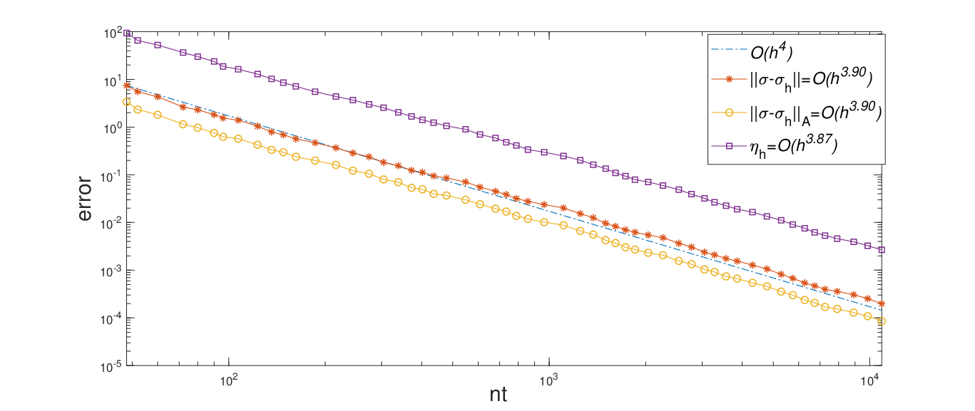
as the exact solution in the test problem. The boundary condition is based on pure displacement (ΓN=∅\Gamma_{N}=\emptyset). The Lamé constants are λ=104\lambda=10^{4} and μ=1.\mu=1. The method (1.4) or (6.1) is implemented using the package iFEM [17] in Matlab 2019a. We start with the initial mesh in Figure 1 and set the marking parameter θ=0.3\theta=0.3. The algebraic system (6.3) is solved by the conjugate gradient method preconditioned by the incomplete Cholesky decomposition. Numerical results are presented in Figure 2, where nt denotes the number of triangles.

It can be observed from Figure 1(right) that the adaptive algorithm 4.1 captures the corner singularity. Figure 2 shows that Algorithm 4.1 has optimal and robust rate of convergence with respect to very large Lamé constant λ\lambda starting from coarse initial grid, which validates our convergence and complexity analysis.

Refer to caption
Figure 1. (left)Initial grid. (right)Adaptive grid, 5290 elements.
Refer to caption
Figure 2. Error curve

Acknowledgements

The author would like to thank Dr. Shihua Gong for generously sharing his Matlab code and comments on iterative methods.

References

  • [1] Douglas N. Arnold, Gerard Awanou, and Ragnar Winther, Finite elements for symmetric tensors in three dimensions, Math. Comp. 77 (2008), no. 263, 1229–1251.
  • [2] Douglas N. Arnold and Franco Brezzi, Mixed and nonconforming finite element methods: implementation, postprocessing and error estimates, RAIRO Modél. Math. Anal. Numér. 19 (1985), no. 1, 7–32. MR 813687
  • [3] Douglas N. Arnold, Jim Douglas, Jr., and Chaitan P. Gupta, A family of higher order mixed finite element methods for plane elasticity, Numer. Math. 45 (1984), no. 1, 1–22. MR 761879
  • [4] Douglas N. Arnold and Ragnar Winther, Mixed finite elements for elasticity, Numer. Math. 92 (2002), no. 3, 401–419.
  • [5] Eberhard Bänsch, Local mesh refinement in 2 and 3 dimensions, Impact Comput. Sci. Engrg. 3 (1991), no. 3, 181–191.
  • [6] Roland Becker and Shipeng Mao, An optimally convergent adaptive mixed finite element method, Numer. Math. 111 (2008), no. 1, 35–54.
  • [7] Peter Binev, Wolfgang Dahmen, and Ron DeVore, Adaptive finite element methods with convergence rates, Numer. Math. 97 (2004), no. 2, 219–268.
  • [8] Susanne C. Brenner, Korn’s inequalities for piecewise H1{H}^{1} vector fields, Math. Comp. 73 (2003), no. 247, 1067–1087.
  • [9] Susanne C. Brenner and L. Ridgway Scott, The mathematical theory of finite element methods, 3 ed., Texts in Applied Mathematics, 15, vol. 35, Springer, New York, 2008.
  • [10] C. Carstensen, A unifying theory of a posteriori finite element error control, Numer. Math. 100 (2005), no. 4, 617–637. MR 2194587
  • [11] C. Carstensen, M. Feischl, M. Page, and D. Praetorius, Axioms of adaptivity, Comput. Math. Appl. 67 (2014), no. 6, 1195–1253. MR 3170325
  • [12] Carsten Carstensen and Georg Dolzmann, A posteriori error estimates for mixed FEM in elasticity, Numer. Math. 81 (1998), no. 2, 187–209.
  • [13] Carsten Carstensen, Dietmar Gallistl, and Joscha Gedicke, Residual-based a posteriori error analysis for symmetric mixed Arnold-Winther FEM, Numer. Math. 142 (2019), no. 2, 205–234.
  • [14] Carsten Carstensen and R. H. W. Hoppe, Error reduction and convergence for an adaptive mixed finite element method, Math. Comp. 75 (2006), no. 255, 1033–1042.
  • [15] Carsten Carstensen and Hella Rabus, The adaptive nonconforming FEM for the pure displacement problem in linear elasticity is optimal and robust, SIAM J. Numer. Anal. 50 (2012), no. 3, 1264–1283.
  • [16] J. Manuel Cascon, Christian Kreuzer, Ricardo H. Nochetto, and Kunibert G. Siebert, Quasi-optimal convergence rate for an adaptive finite element method, SIAM J. Numer. Anal. 46 (2008), no. 5, 2524–2550.
  • [17] Long Chen, iFEM: an innovative finite element method package in Matlab, University of California Irvine, Technical report, 2009.
  • [18] Long Chen, Michael Holst, and Jinchao Xu, Convergence and optimality of adaptive mixed finite element methods, Math. Comp. 78 (2009), no. 265, 35–53.
  • [19] Long Chen, Jun Hu, and Xuehai Huang, Fast auxiliary space preconditioners for linear elasticity in mixed form, Math. Comp. 78 (2018), no. 312, 1601–1633.
  • [20] Long Chen, Jun Hu, Xuehai Huang, and Hongying Man, Residual-based a posteriori error estimates for symmetric conforming mixed finite elements for linear elasticity problems, Sci. China Math. 61 (2018), no. 6, 973–992.
  • [21] Lars Diening, Christian Kreuzer, and Rob Stevenson, Instance optimality of the adaptive maximum strategy, Found. Comput. Math. 16 (2016), no. 1, 33–68.
  • [22] Willy Dörfler, A convergent adaptive algorithm for Poisson’s equation, SIAM J. Numer. Anal. 33 (1996), no. 3, 1106–1124. MR 1393904
  • [23] M. Feischl, T. Führer, and D. Praetorius, Adaptive FEM with optimal convergence rates for a certain class of nonsymmetric and possibly nonlinear problems, SIAM J. Numer. Anal. 52 (2014), no. 2, 601–625.
  • [24] V. Girault and L. R. Scott, Hermite interpolation of nonsmooth functions preserving boundary conditions, Math. Comp. 71 (2002), no. 239, 1043–1074.
  • [25] Shihua Gong, Shuonan Wu, and Jinchao Xu, New hybridized mixed methods for linear elasticity and optimal multilevel solvers, Numer. Math. 141 (2019), 569–604.
  • [26] Pierre Grisvard, Singularities in boundary value problems, Research in Applied Mathematics, 22, Springer-Verlag, Berlin, 1992.
  • [27] Michael Holst, Yuwen Li, Adam Mihalik, and Ryan Szypowski, Convergence and optimality of adaptive mixed methods for Poisson’s equation in the FEEC framework, J. Comp. Math. 38 (2020), no. 5, 748–767.
  • [28] Jun Hu, Finite element approximations of symmetric tensors on simplicial grids in ℝn\mathbb{R}^{n}: the higher order case, J. Comput. Math. 33 (2015), no. 3.
  • [29] Jun Hu and Rui Ma, Partial relaxation of C0C^{0} vertex continuity of stresses of conforming mixed finite elements for the elasticity problem, Comput. Methods Appl. Math. 21 (2021), no. 1, 89–108. MR 4193452
  • [30] Jun Hu and Shangyou Zhang, A family of conforming mixed finite elements for linear elasticity on triangular grids, arXiv:1406.7457, 2014.
  • [31] Jianguo Huang and Yifeng Xu, Convergence and complexity of arbitrary order adaptive mixed element methods for the poisson equation, Sci. China Math. 55 (2012), no. 5, 1083–1098.
  • [32] Yuwen Li, Some convergence and optimality results of adaptive mixed methods in finite element exterior calculus, SIAM J. Numer. Anal. 57 (2019), no. 4, 2019–2042. MR 3995302
  • [33] Yuwen Li, Quasi-optimal adaptive mixed finite element methods for controlling natural norm errors, Math. Comp. 90 (2021), 565–593.
  • [34] Yuwen Li and Ludmil Zikatanov, Nodal auxiliary a posteriori error estimates, arXiv preprint, arXiv:2010.06774 (2020).
  • [35] Marco Lonsing and Rüdiger Verfürth, A posteriori error estimators for mixed finite element methods in linear elasticity, Numer. Math. 97 (2004), no. 4, 757–778. MR 2127931
  • [36] William F. Mitchell, A comparison of adaptive refinement techniques for elliptic problems, ACM Trans. Math. Software 15 (1989), no. 4, 326–347.
  • [37] John Morgan and Ridgway Scott, A nodal basis for C1{C}^{1} piecewise polynomials of degree n≥5n\geq 5, Math. Comput. 29 (1975), 736–740.
  • [38] Pedro Morin, Ricardo H. Nochetto, and Kunibert G. Siebert, Data oscillation and convergence of adaptive FEM, SIAM J. Numer. Anal. 38 (2000), no. 2, 466–488.
  • [39] Rob Stevenson, Optimality of a standard adaptive finite element method, Found. Comput. Math. 7 (2007), no. 2, 245–269.
  • [40] by same author, The completion of locally refined simplicial partitions created by bisection, Math. Comp. 77 (2008), no. 261, 227–241.
  • [41] Rüdiger Verfürth, A posteriori error estimation techniques for finite element methods, Numerical Mathematics and Scientific Computation, Oxford University Press, Oxford, 2013. MR 3059294