With or without ? Probing non-standard flavor
and helicity structures in
semileptonic decaysPreprint: ZU-TH-42/19
Abstract
Motivated by the recent hints of lepton flavor universality violation observed in semileptonic decays, we analyze how to test flavor and helicity structures of the corresponding amplitudes in view of future data. We show that the general assumption that such non-standard effects are controlled by a flavor symmetry, minimally broken as in the Standard Model Yukawa sector, leads to stringent predictions on leptonic and semileptonic decays. Future measurements of , , , , , , as well as various polarization asymmetries in decays, will allow to prove or falsify this general hypothesis independently of its dynamical origin.
I Introduction
Present data exhibit intriguing hints of violations of Lepton Flavor Universality (LFU) both in charged-current Aaij et al. 2015a; Lees et al. 2013; Hirose et al. 2017; Aaij et al. 2018; Abdesselam et al. 2019a and neutral-current Aaij et al. 2014; Aaij et al. 2017a; Aaij et al. 2019a; Wei et al. 2009; Abdesselam et al. 2019b; Aubert et al. 2006 semileptonic decays. These hints can be well described employing Effective Field Theory (EFT) approaches (see Bhattacharya et al. 2015; Alonso et al. 2015; Greljo et al. 2015; Calibbi et al. 2015; Barbieri et al. 2016 for the early attempts), whose main ingredients are the assumptions that New Physics (NP) affects predominantly semileptonic operators, and that it couples in a non-universal way to different fermion species. In particular, NP should have dominant couplings to third generation fermions and smaller, but non-negligible, couplings to second generation fermions. Interestingly enough, this non-trivial flavor structure resemble the hierarchies observed in the Standard Model (SM) Yukawa couplings, opening the possibility of a common explanation for the two phenomena.
An effective approach to address the question of a possible connection between the LFU anomalies and the SM Yukawa couplings and, more generally, to investigate the flavor structure of non-standard effects at low-energies, is the assumption of an appropriate flavor symmetry and a set of symmetry-breaking terms. The flavor symmetry does not need to be a fundamental property of the underlying theory, it could simply be an accidental low-energy property. Still, its use in the EFT context provides a very powerful organizing principle for a bottom-up reconstruction of the underlying dynamics.
In the context of the recent anomalies, the flavor symmetry that emerges as particularly suitable to describe the observed data is , which is a subset of the larger proposed in Barbieri et al. 2011; Blankenburg et al. 2012; Barbieri et al. 2012 as a useful organizing principle to address the hierarchies in the SM Yukawa couplings and, at the same time, allow large NP effects in processes involving third-generation fermions (as expected in most attempts to address the electroweak hierarchy problem).
The scope of the present paper is a systematic investigation of the consequences of this symmetry hypothesis in (semi)leptonic decays. Contrary to previous analyses, where this symmetry has been implemented in the context of specific new-physics models, our goal here is to investigate the consequences of this symmetry (and symmetry-breaking) ansatz in general terms, with a minimal set of additional assumptions about the dynamical origin of the anomalies. As we will show, in the case of charged-current interactions, the symmetry ansatz alone is sufficient to derive an interesting series of testable predictions. The predictive power is smaller for neutral-current transitions, but also in that case we can identify a few clean predictions which are direct consequences of the symmetry ansatz alone.
II The symmetry in the SM
The symmetry is the global symmetry that the SM Lagrangian exhibits in the limit where we neglect all entries in the Yukawa couplings but for third generation masses Barbieri et al. 2011; Blankenburg et al. 2012; Barbieri et al. 2012. Under this symmetry, the first two SM fermion families transform as doublets of a given subgroup,
| (1) |
while third-generation quarks (leptons) are only charged under . The largest breaking of this symmetry in the complete SM Lagrangian is controlled by the small parameter
| (2) |
A minimal set of breaking terms (spurions) which lets us reproduce all the observable SM flavor parameters (in the limit of vanishing neutrino masses), without tuning and with minimal size for the breaking terms, is
| (3) |
In terms of these spurions, the Yukawa matrices can be decomposed as
| (4) |
where and are free complex parameters, expected to be of .11 1 In models with more than one Higgs doublet, the smallness of can be justified in terms of approximate flavor-independent symmetries. Note that are complex matrices, while are 2-dimensional complex vectors.
The precise size of the spurions is not known; however, we can estimate it by the requirement of no tuning in the parameters. This implies . In the limit of vanishing neutrino masses, the size of cannot be unambiguously determined. As discussed below (see also Cornella et al. 2019), a good fit of the anomalies in semileptonic decays is obtained for
| (5) |
which is perfectly consistent with: i) the estimate ; ii) the hypothesis of a common origin for the two leading breaking terms in quark and lepton sectors. The entries in the matrices are significantly smaller than , with a maximal size of in the quark sector.
By appropriate field redefinitions and without loss of generality, one can remove unphysical parameters in the Yukawa matrices in (4) (see App. A). Working in the so-called interaction basis, where the second generation in space is defined by the alignment of the leading spurions,
| (6) |
one can bring the Yukawa matrices to the following form
| (7) |
where are diagonal positive matrices, are orthogonal matrices and is of the form
| (8) |
with and .
The Yukawa matrices in (7) get diagonalized by means of appropriate unitary transformations: , with . The most general form for these unitary transformations is
| (9) |
with . Here we have taken advantage of the constraints imposed by fermions masses and CKM matrix elements to eliminate various parameters appearing in and .22 2 The removal of unphysical parameters presented in App. A corrects a similar analysis presented in Bordone et al. 2018, where it was erroneously concluded that the parameter is unconstrained. These further imply that and are constrained by and , and that . The light-family leptonic mixing (), appearing in , cannot be expressed in terms of measurable quantities. Two additional mixing angles which remain unconstrained are and . Finally, is an unconstrained phase, that becomes unphysical in the limit (or, equivalently, ). This limit is phenomenologically required in models where operators are generated at tree-level around the TeV scale: in such case one needs to impose a mild alignment to the down basis, i.e. , to satisfy the constraints from -meson mixing Di Luzio et al. 2017; Bordone et al. 2018; Di Luzio et al. 2018.
III Impact of on the EFT for semileptonic decays
Having defined the flavor symmetry and its symmetry breaking terms from the SM Yukawa sector, we are ready to analyze its implications beyond the SM. Assuming no new degrees of freedom below the electroweak scale, we can describe NP effects in full generality employing the so-called SMEFT. We limit the attention to dimension-six four-fermion operators bilinear in quark and lepton fields,33 3 We neglect operators which modify the effective couplings of and bosons. These are highly constrained and cannot induce sizable LFU violating effects. that we write generically as
| (10) |
where GeV is the SM Higgs vev, are lepton-flavor indices, and are quark-flavor indices. The operators in the Warsaw basis Grzadkowski et al. 2010 with a non-vanishing tree-level matrix element in semileptonic decays are
| (11) |
where are the Pauli matrices and are indices. Our main hypothesis is to reduce the number of retaining only those corresponding to invariant operators, up to the insertion of one or two powers of the leading spurions in (5).
A first strong simplification arises by neglecting subleading spurions with non-trivial transformation properties under . Since we are interested in processes of the type and , this implies that only the operators , , and can yield a relevant contribution. Among those, can significantly contribute at tree-level only to transitions: since the latter are currently poorly constrained (see sect. IV.3), we do not consider this operator for simplicity. We are thus left with the following effective Lagrangian
| (12) |
where control the overall strength of the NP effects and are tensors that parametrize the flavor structure. They are normalized by setting , which is the only term surviving in the exact limit.
Let us consider first the structure of , which is particularly simple. Neglecting breaking spurions, it factorizes to
| (13) |
where, in the interaction basis,
| (14) |
Here are coefficients and we have neglected higher-order terms in (that would simply redefine such coefficients). Moving to the mass-eigenstate basis of down quarks and charged leptons, where
| (15) |
we have and [see (9)], with the new matrices assuming the following explicit form in notation
| (16) |
The (complex) parameters , , , and are a combination of the spurions in (14) and the rotation terms from , that satisfy
| (17) |
On the r.h.s. of the first line of (III) we have neglected tiny terms suppressed by more than two powers of or .
If we consider at most one power of and one power of , then also factorizes into
| (18) |
where and have the same structure as with, a priori, different coefficients for the spurions. Moving to the basis (15), assumes the same structure as in (III), with parameters which can differ by O(1) overall factors, but that obey the same flavor ratios as in (III). Corrections to the factorized structure in (18) arises only to second order in or , generating terms which are either irrelevant or can be reabsorbed in a redefinition of the observable parameters in the processes we are interested in (see sect. IV).
III.1 Matching to the leptoquark case
The EFT in (12), with factorized flavor couplings as in (13) and (18), nicely matches the structure generated by integrating out a vector leptoquark, transforming as under the SM gauge group. As noted first in Barbieri et al. 2016, this field provides indeed an excellent mediator to build in a natural, and sufficiently general way, an EFT for semileptonic decays built on the flavor symmetry broken only by the leading and spurions (see Bhattacharya et al. 2017; Di Luzio et al. 2017; Hiller and Nisandzic 2017; Buttazzo et al. 2017; Bordone et al. 2018; Angelescu et al. 2018; Kumar et al. 2019; Di Luzio et al. 2018; Aebischer et al. 2019; Cornella et al. 2019 for other phenomenological analysis of the leptoquark in physics).
Writing the interaction between the field and SM fermions in the basis of (15) as Cornella et al. 2019
| (19) |
the flavor symmetry hypothesis imply a parametric structure for and identical to that of and in (III). Normalizing such that , and integrating out the field, leads to the following (tree-level) matching conditions for the parameters of
| (20) |
and
| (21) |
where . Note that while (21) is just a redefinition of the free parameters of the effective Lagrangian, (20) give non-trivial constraints. We also stress that, beside the overall coupling (encoded in ) the four combinations of couplings in (21) indicate the helicity structure of the interactions () and its alignment in quark and lepton flavor space (, and ).
The condition , arising naturally in the case, is important to evade the tight constraints on from observables and electroweak precision tests Buttazzo et al. 2017. In order to analyze charged currents as much independent as possible from other observables, we take in the Lagrangian in (12). Similarly, we set in order to avoid the introduction of redundant parameters as far as neutral currents are concerned.
IV The relevant observables
IV.1 rates and polarization asymmetries
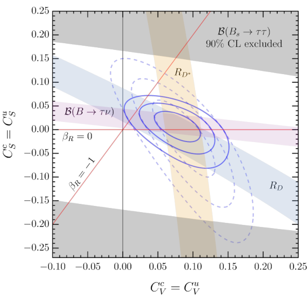
At fixed quark and lepton flavors, the effective Lagrangian in (12) depends only on two coefficients. In the case, we conveniently re-define them as
| (22) |
where, in the last line, we have used CKM unitarity. When defining , we have factorized the CKM factor , such the that the left-handed part of the interactions is modified as
| (23) |
In the absence of the simplifying hypothesis , one would need to redefine replacing with . Employing this hypothesis, as in the leptoquark case, the ratio is flavor blind and depends only on the helicity structure of the NP amplitude.
Using the results in Bernlochner et al. 2017; Tanaka and Watanabe 2013 for the form factors and decay rates, and neglecting the tiny NP corrections in the case (see below) leads to the following expression for the LFU ratios, ,
| (24) |
where arises from the running of the scalar operator from the TeV scale down to González-Alonso et al. 2017. Updated SM predictions for can be found in Bordone et al. 2019:
| (25) |
Current measurements of and Aaij et al. 2015a; Lees et al. 2013; Hirose et al. 2017; Aaij et al. 2018; Abdesselam et al. 2019a lead to the constraints on and shown in Fig. 1 (dashed contour lines) where, for simplicity, we have assumed these couplings to be real. For comparison, the directions corresponding to a pure left-handed () or a vector-like interaction () for the are also indicated.
Before discussing the impact of additional observables in constraining the same set of parameters (under additional assumptions), we stress that once and have been determined, all the other observables are completely fixed by the invariant structure of and can be used to test it. Particularly interesting in this respect are the polarization asymmetries,
| (26) | |||||
where the denotes a with helicity. We find the following expressions for these observables44 4 The numerical coefficients in (28) are compatible with those obtained in Iguro et al. 2019, within the errors, and are within of to those obtained in Blanke et al. 2019 (where different form factors have been employed).
| (27) |
Taking real for simplicity, we obtain
| (28) |
where Bordone et al. 2019
| (29) |
Since the effect of is that of rescaling the SM amplitude, all the above ratios are largely insensitive to the value of and become 1 in the limit .
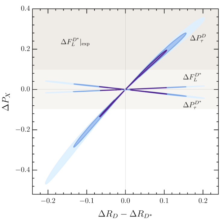
This fact is clearly illustrated in Fig. 2, where we plot the deviations from unity of the polarization ratios vs. the difference on the two leading LFU ratios (which also vanishes in the limit ),
| (30) |
As can be seen, the predicted pattern of deviations is very precise and rather specific. At present, only Hirose et al. 2017; Hirose et al. 2018 and Abdesselam et al. 2019c have been measured, still with large uncertainties. As shown in Fig. 2, it is not possible in our setup to reach the current experimental central value for (see Iguro et al. 2019; Murgui et al. 2019 for a similar discussion).
The last observable we take into account is , that is particularly sensitive to the scalar amplitude. Despite it will be quite difficult to measure this branching ratio in the future, interesting bounds can be derived from the measurement of the lifetime Alonso et al. 2017; Celis et al. 2017a. The expression for this observable reads
| (31) |
where , . We find to be at most at the level of for the best fit contours in Fig. 1, well below the bound obtained in Alonso et al. 2017.
In principle, additional probes of the amplitude are provided by the LFU ratios in Blanke et al. 2019 and in Watanabe 2018 decays. In both cases scalar amplitudes are subleading and, in our framework, one should expect an enhancement compared to the SM prediction similar to the one occurring in . However, measuring the LFU ratio in –where we have a precise SM prediction Detmold et al. 2015– is quite challenging, while in the case the current SM theory error is well above the level Cohen et al. 2018.
IV.2 transitions
The analog of for transitions are the effective couplings
| (32) |
where the result in the second line follows from CKM unitarity. The prediction of same size NP effects, relative to the SM, in and transitions is a distinctive feature of the minimally-broken hypothesis.
At present, the most significant constrains on transitions are derived from , whose branching ratio is
| (33) |
where and Bona 2017. The continuous contour lines in Fig. 1 show the constraints on and once the experimental data on are combined with those on Tanabashi et al. 2018 ( range indicated by the purple band in Fig. 1).
In the future, very interesting constraints are expected from . Using the hadronic parameters in Tanaka and Watanabe 2017; Bailey et al. 2015a, we find for
| (34) |
where Bernlochner 2015; Du et al. 2016; Tanaka and Watanabe 2017. In the limit where quadratic NP effects can be neglected, the following approximate relation holds
| (35) |
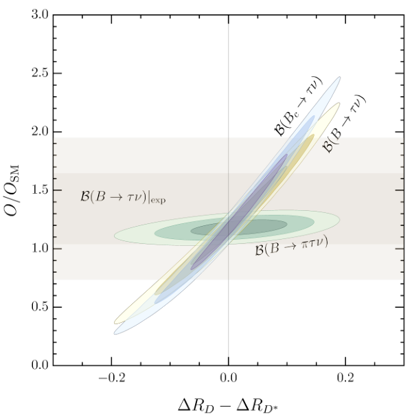
which would allow a non-trivial test of the structure of the interactions. In Fig. 3 we show the predictions for , , and , as a function of . As shown in the figure, our setup predicts also
| (36) |
where the difference among the two modes arises by sub-leading spectator mass effects in the chirality-enhacement factors and .
IV.3 transitions
The semileptonic transitions have a rich phenomenology and have been extensively discussed in the recent literature. Contrary to the charged-current case, here model-dependent assumptions, such as the constraints in (20), play a more important role. Rather than presenting a comprehensive analysis of the various observables accessible in these modes, our scope here is to focus on: i) model-independent predictions related to the minimally-broken hypothesis; ii) clean observables controlling the size of the symmetry breaking terms.
.
Under the assumption , following from the hypothesis of a UV-completion, NP effects in transitions are forbidden at tree level. On the other hand, NP contributions to are almost as large as those in for (see e.g. Buttazzo et al. 2017; Capdevila et al. 2018a). The most relevant observable involving these transitions is , which could receive a sizable chiral enhancement:
| (37) |
where and (see below). The enhancement of this rate compared to the SM expectation could reach a factor of () for (. However, the current experimental limit Aaij et al. 2017b; Bobeth et al. 2014
| (38) |
is still well below the possible maximal enhancement. As a result, at present this observable does not put stringent constraints on the parameter space of the EFT: in Fig. 1 we show the CL exclusion region in the plane for .
As pointed out in Crivellin et al. 2019, a possible large enhancement of the amplitude can indirectly be tested via the one-loop-induced lepton-universal contributions to in the direction (see below). This contribution is well compatible and even favored by current data Algueró et al. 2019; Aebischer et al. 2019.
.
FCNC decays to light leptons offer an excellent probe of the breaking terms in the lepton sector. These transitions are commonly described in terms of the so-called weak effective Hamiltonian Grinstein et al. 1988; Buchalla et al. 1996
| (39) |
with the Fermi constant, the fine-structure constant and
| (40) |
In the SM, , and . Matching to the Lagrangian in (12), we get ()
| (41) |
while the corresponding tree-level effects in the electron sector are negligible.
One of most relevant observables involving these transitions are the LFU ratios , which are particular interesting due to their robust theoretical predictions: Bordone et al. 2016. In our setup, one gets Celis et al. 2017b; Capdevila et al. 2018b
| (42) |
The prediction , is a direct consequence of our flavor symmetry assumptions and is independent of the initial set of dimension-six SMEFT operators. As observed first in Hiller and Schmaltz 2015, the relation holds in any NP model where LFU contributions to decays are induced by a left-handed quark current: in our framework this is a direct consequence of the smallness of the flavor-symmetry breaking terms in the right-handed sector. From the experimental point of view, this implies that all universality ratios in transitions are expected to be the same, provided their SM contribution is dominated by and/or . In addition to (42), we thus expect55 5 We define the universality ratios as , assuming a region in below the charmonium resonances and sufficiently above the di-muon threshold GeV).
| (43) |
Current experimental data hint to sizable NP effects in and Aaij et al. 2017a; Aaij et al. 2019a; Wei et al. 2009; Abdesselam et al. 2019b; Aubert et al. 2006, consistent with .
Assuming the NP effect to be the same in and , the combined measurements imply (corresponding to ). This numerical value provides an important contraint on the size of the leptonic spurion (): since , setting and , as suggested by the fit, the value of implies . Within the UV leptoquark completion, the fact that allows us also to determine a non-trival relative sign among the breking terms: according to (20) one has , which implies .
Other data involving transitions, such as the measurements of Aaij et al. 2016; Wehle et al. 2017; Aaboud et al. 2018; Chatrchyan et al. 2017 and other differential distributions, also deviate from the SM predictions consistently with , further supporting the hypothesis of . This coincidence in size for quark and lepton spurions points to the interesting possibility of a common origin for the two leading breaking terms.
.
Among transitions, a special role is played by , where the chiral enhancement of the scalar amplitude allows us to probe the helicity structure of the NP interaction. The branching ratio normalised to the SM value reads
| (44) |
Expressing the deviations in the Wilson coefficients in terms of , by means of (41) and (42), leads to
| (45) |
Current experimental measurements Aaboud et al. 2019; Chatrchyan et al. 2013; Khachatryan et al. 2015; Aaij et al. 2017c; CMS 2019 yield
| (46) |
which is about below the SM expectation: Beneke et al. 2019. In Fig. 4, we show the predictions for this observable as a function of for (purple band), and for setting (green band). As can be seen, the deviations in are well compatible with the current experimental values of and, if is large, small values of are favored.
.
As far as LFV processes are concerned, the most relevant observable is
| (47) |
As in , the large chiral enhancement of the scalar contribution make it an excellent probe of the helicity structure of the NP effects. Moreover, this observable provides a direct probe of . Setting and , we find , while for and the same values of the other NP parameters, the expected branching fraction is about one order of magnitude smaller. The current experimental limit, Aaij et al. 2019b, is close to the NP predictions when is sizable. Future improvements in this observable will therefore provide very significant constraints.
IV.4 and other FCNCs
A key prediction of the minimally broken framework is that NP effects in and transitions scale according to the corresponding CKM factors. More precisely, defining the effective hamiltonian of the leading FCNC operators as
| (48) |
where , then it is easy to check that, because of (III),
| (49) |
These relations lead to a series of accurate predictions which could be tested in various observables.
One of the cleanest test is obtained by means of decays, where we expect
| (50) |
where denotes an interval in where perturbative contributions are dominant.66 6 The regions where perturbative contributions dominates over charmonia or light resonance terms are the low- region () and the high- region (). The SM prediction for the rate is Khodjamirian and Rusov 2017 and Bailey et al. 2015b, to be compared with the LHCb results and Aaij et al. 2015b. These measurements deviate from the SM predictions by and , respectively, and are well consistent with (50) (assuming NP effect in the mode to be subleading), although they are still affected by large errors. Similarly, our framework predicts
| (51) |
Leaving aside decays, the effective Lagrangian (12) necessarily imply non-standard effects also in and semileptonic decays. Since NP effects in these processes are strongly constrained, it is important to check if these constraints limit the parameter space of the EFT. As far as decays are concerned, the most stringent constraint is obtained by the non-observation of . Only the chiral-enhanced contribution to , proportional to , can be reliably estimated in the EFT, yielding77 7 The full branching fraction, including both vector and non-chiral-enhanced scalar contributions, was computed in Cornella et al. 2019 in a specific UV-completion. There, it was found that the additional contributions are much smaller than the ones quoted here if .
| (52) |
Taking and , we find , which is below current bounds but within the expected Belle II sensitivity Altmannshofer et al. 2018.
Finally, the constraints obtained from decays do not yield significant bounds to our framework. As in the case, NP effects in transitions are forbidden at tree-level if we take . On the other hand, decays receive strong spurion suppressions, resulting in bounds on that are significantly above the preferred values. These are shown in Table 1, together with the parametric spurion dependence of the corresponding transition. For comparison, we stress that the preferred value of emerging from the fit in Fig. 1, assuming , is .
| Process | Spurion comb. for | Bound on |
|---|---|---|
IV.5 Charged-current transitions to light leptons
The breaking in the lepton sector could in principle be tested also in charged-current decays to light leptons, both in and transitions. The most relevant observables in each category are respectively and , whose experimental measurements will be improved at Belle II Altmannshofer et al. 2018. In contrast to , scalar contributions to are extremely suppressed due to the flavor symmetry [see (III)].
The LFU ratios can be expressed as
| (53) |
where the first term corresponds to the mode with and the second one with and where, similarly to , we have defined
| (54) |
Taking , and , we find that NP corrections to these observables are at most at the per-mille level, hence beyond the near-future experimental sensitivity. This is quite different from what is expected in other NP models addressing the anomalies, such as the scalar leptoquark models considered in Doršner et al. 2017; Bečirević et al. 2018.
It is also worth stressing that the phenomenological condition , required to accommodate with , yields a partial cancellation between the two terms in . As a result of this cancellation, NP effects are typically at the sub per-mille level, hence beyond any realistic sensitivity even in a long-term perspective. Similarly, we find possible NP contributions to to be at or below the per-mille level, very far from the experimental reach.
V Conclusions
The hints of LFU violations observed in meson decays have shaken many prejudices about physics beyond the SM, opening new directions in model building. One of the most intriguing possibilities is the existence of a link between the (non-standard) dynamics responsible for these anomalies and that responsible for the fermion mass hierarchies. A specific realization of this idea is the hypothesis that, at low energies, the new dynamics manifests via an EFT controlled by an approximate symmetry, with leading breaking in specific directions in the and subgroups.
In this paper we have explored in generality the consequences of this symmetry and symmetry-breaking hypothesis in (semi)leptonic decays, trying to avoid making additional dynamical assumptions about the origin of the anomalies. As we have shown, the symmetry hypothesis alone leads to a significant reduction in the number of free parameters of the EFT which, in turn, can be translated into stringent predictions on various low-energy observables. The situation is particularly simple in the case of charged currents, where all relevant processes are controlled by two independent combinations of effective couplings. The latter can be determined for instance from and , leading to a series of unambiguous predictions for , , polarization asymmetries in , as well as other processes. As shown in Fig. 1, the available data on perfectly support the initial hypothesis.
In neutral currents, additional combinations of effective couplings appear, but also in this case a series of stringent predictions, which are genuine consequences of the symmetry and symmetry-breaking hypothesis alone, can be derived. The two most notable ones are: i) the (approximate) universality of the deviations from 1 in ratios in short-distance dominated trasitions, leading to (43), and ii) the SM-like CKM scaling of NP effects in and transitions, which leads to the relations (50) and (51). If the significance of the current anomalies will increase, the experimental tests of these relations, which are within the reach of current facilities, will provide an invaluable help in clarifying the origin of this intriguing phenomenon.
Acknowledgements
We thank Ryotaro Watanabe for fruitful discussions. This project has received funding from the European Research Council (ERC) under the European Union’s Horizon 2020 research and innovation programme under grant agreement 833280 (FLAY), and by the Swiss National Science Foundation (SNF) under contract 200021-159720. The work of J.F. was also supported in part by the Generalitat Valenciana under contract SEJI/2018/033. The work of K.Y. was also supported in part by the JSPS KAKENHI 18J01459.
Appendix A Physical parameters in the spurions
We describe here how to remove the unphysical parameters in the spurions appearing in (4). Let us focus first on the quark sector. In the exact limit, the Lagrangian presents a
| (55) |
flavor symmetry. Since, by assumption, this symmetry is only broken by and , field transformations under this symmetry only modify these spurions. In particular, the transformation88 8 We use the subscript to denote first- and second-generation fermions.
| (56) |
with being general unitary matrices, let us bring to the following form
| (57) |
Here are diagonal positive matrices and is an orthogonal matrix. This is the well-known result that in the SM with two families, only the Cabbibo matrix is physical and there are no observable CP-violating phases. A residual symmetry, corresponding to baryon number for light quarks, remains unbroken by these spurions. In terms of degrees of freedom, we started with 8 real parameters and 8 phases in , and we used the full freedom of the symmetry to remove parameters. In the end, real parameters remain: quark masses and one mixing angle.
The field redefinitions performed so far also redefine the spurion: . We can decompose it as
| (58) |
with defined as in (8). Without loss of generality, the phase can be absorbed into a redefinition of . Moreover, we can use the symmetry transformation to remove one phase combination from the two phases in . We use this freedom to set equal phases for and . Finally, we can absorb the phase of into a redefinition of the and fields. This final redefinition modifies the phase of any -preserving NP interaction, but it does not affect the rest of the SM Lagrangian. After all these field transformations, we end up with the following quark Yukawa matrices
| (59) |
A final transformation, , is sufficient to bring these matrices to the form in (7).
The same procedure can be applied to the lepton sector, however in this case there are three differences with respect to the quark case (in the limit of vanishing neutrino masses): i) a subgroup of the symmetry is enough to make diagonal and positive, with no extra orthogonal matrices; ii) the remaining freedom let us reduce to an orthogonal matrix, which we denote as ; iii) the transformation can be used to remove the phase in , leaving no free phases. After an appropriate transformation, it is straightforward to arrive to the form in (7).
References
- Aaij et al. (2015a) R. Aaij et al. (LHCb), Phys. Rev. Lett. 115, 111803 (2015a), [Erratum: Phys. Rev. Lett.115,no.15,159901(2015)], arXiv:1506.08614 [hep-ex] .
- Lees et al. (2013) J. P. Lees et al. (BaBar), Phys. Rev. D88, 072012 (2013), arXiv:1303.0571 [hep-ex] .
- Hirose et al. (2017) S. Hirose et al. (Belle), Phys. Rev. Lett. 118, 211801 (2017), arXiv:1612.00529 [hep-ex] .
- Aaij et al. (2018) R. Aaij et al. (LHCb), Phys. Rev. D97, 072013 (2018), arXiv:1711.02505 [hep-ex] .
- Abdesselam et al. (2019a) A. Abdesselam et al. (Belle), (2019a), arXiv:1904.08794 [hep-ex] .
- Aaij et al. (2014) R. Aaij et al. (LHCb), Phys. Rev. Lett. 113, 151601 (2014), arXiv:1406.6482 [hep-ex] .
- Aaij et al. (2017a) R. Aaij et al. (LHCb), JHEP 08, 055 (2017a), arXiv:1705.05802 [hep-ex] .
- Aaij et al. (2019a) R. Aaij et al. (LHCb), Phys. Rev. Lett. 122, 191801 (2019a), arXiv:1903.09252 [hep-ex] .
- Wei et al. (2009) J. T. Wei et al. (Belle), Phys. Rev. Lett. 103, 171801 (2009), arXiv:0904.0770 [hep-ex] .
- Abdesselam et al. (2019b) A. Abdesselam et al. (Belle), (2019b), arXiv:1904.02440 [hep-ex] .
- Aubert et al. (2006) B. Aubert et al. (BaBar), Phys. Rev. D73, 092001 (2006), arXiv:hep-ex/0604007 [hep-ex] .
- Bhattacharya et al. (2015) B. Bhattacharya, A. Datta, D. London, and S. Shivashankara, Phys. Lett. B742, 370 (2015), arXiv:1412.7164 [hep-ph] .
- Alonso et al. (2015) R. Alonso, B. Grinstein, and J. Martin Camalich, JHEP 10, 184 (2015), arXiv:1505.05164 [hep-ph] .
- Greljo et al. (2015) A. Greljo, G. Isidori, and D. Marzocca, JHEP 07, 142 (2015), arXiv:1506.01705 [hep-ph] .
- Calibbi et al. (2015) L. Calibbi, A. Crivellin, and T. Ota, Phys. Rev. Lett. 115, 181801 (2015), arXiv:1506.02661 [hep-ph] .
- Barbieri et al. (2016) R. Barbieri, G. Isidori, A. Pattori, and F. Senia, Eur. Phys. J. C76, 67 (2016), arXiv:1512.01560 [hep-ph] .
- Barbieri et al. (2011) R. Barbieri, G. Isidori, J. Jones-Perez, P. Lodone, and D. M. Straub, Eur. Phys. J. C71, 1725 (2011), arXiv:1105.2296 [hep-ph] .
- Blankenburg et al. (2012) G. Blankenburg, G. Isidori, and J. Jones-Perez, Eur. Phys. J. C72, 2126 (2012), arXiv:1204.0688 [hep-ph] .
- Barbieri et al. (2012) R. Barbieri, D. Buttazzo, F. Sala, and D. M. Straub, JHEP 07, 181 (2012), arXiv:1203.4218 [hep-ph] .
- Cornella et al. (2019) C. Cornella, J. Fuentes-Martin, and G. Isidori, JHEP 07, 168 (2019), arXiv:1903.11517 [hep-ph] .
- Bordone et al. (2018) M. Bordone, C. Cornella, J. Fuentes-Martín, and G. Isidori, JHEP 10, 148 (2018), arXiv:1805.09328 [hep-ph] .
- Di Luzio et al. (2017) L. Di Luzio, A. Greljo, and M. Nardecchia, Phys. Rev. D96, 115011 (2017), arXiv:1708.08450 [hep-ph] .
- Di Luzio et al. (2018) L. Di Luzio, J. Fuentes-Martin, A. Greljo, M. Nardecchia, and S. Renner, JHEP 11, 081 (2018), arXiv:1808.00942 [hep-ph] .
- Grzadkowski et al. (2010) B. Grzadkowski, M. Iskrzynski, M. Misiak, and J. Rosiek, JHEP 10, 085 (2010), arXiv:1008.4884 [hep-ph] .
- Bhattacharya et al. (2017) B. Bhattacharya, A. Datta, J.-P. Guévin, D. London, and R. Watanabe, JHEP 01, 015 (2017), arXiv:1609.09078 [hep-ph] .
- Hiller and Nisandzic (2017) G. Hiller and I. Nisandzic, Phys. Rev. D96, 035003 (2017), arXiv:1704.05444 [hep-ph] .
- Buttazzo et al. (2017) D. Buttazzo, A. Greljo, G. Isidori, and D. Marzocca, JHEP 11, 044 (2017), arXiv:1706.07808 [hep-ph] .
- Angelescu et al. (2018) A. Angelescu, D. Bečirević, D. A. Faroughy, and O. Sumensari, JHEP 10, 183 (2018), arXiv:1808.08179 [hep-ph] .
- Kumar et al. (2019) J. Kumar, D. London, and R. Watanabe, Phys. Rev. D99, 015007 (2019), arXiv:1806.07403 [hep-ph] .
- Aebischer et al. (2019) J. Aebischer, W. Altmannshofer, D. Guadagnoli, M. Reboud, P. Stangl, and D. M. Straub, (2019), arXiv:1903.10434 [hep-ph] .
- (31) https://hflav-eos.web.cern.ch/hflav-eos/semi/spring19/html/RDsDsstar/RDRDs.html.
- Bernlochner et al. (2017) F. U. Bernlochner, Z. Ligeti, M. Papucci, and D. J. Robinson, Phys. Rev. D95, 115008 (2017), [erratum: Phys. Rev.D97,no.5,059902(2018)], arXiv:1703.05330 [hep-ph] .
- Tanaka and Watanabe (2013) M. Tanaka and R. Watanabe, Phys. Rev. D87, 034028 (2013), arXiv:1212.1878 [hep-ph] .
- González-Alonso et al. (2017) M. González-Alonso, J. Martin Camalich, and K. Mimouni, Phys. Lett. B772, 777 (2017), arXiv:1706.00410 [hep-ph] .
- Bordone et al. (2019) M. Bordone, M. Jung, and D. van Dyk, (2019), arXiv:1908.09398 [hep-ph] .
- Iguro et al. (2019) S. Iguro, T. Kitahara, Y. Omura, R. Watanabe, and K. Yamamoto, JHEP 02, 194 (2019), arXiv:1811.08899 [hep-ph] .
- Blanke et al. (2019) M. Blanke, A. Crivellin, S. de Boer, T. Kitahara, M. Moscati, U. Nierste, and I. Nišandžić, Phys. Rev. D99, 075006 (2019), arXiv:1811.09603 [hep-ph] .
- Hirose et al. (2018) S. Hirose et al. (Belle), Phys. Rev. D97, 012004 (2018), arXiv:1709.00129 [hep-ex] .
- Abdesselam et al. (2019c) A. Abdesselam et al. (Belle), in 10th International Workshop on the CKM Unitarity Triangle (CKM 2018) Heidelberg, Germany, September 17-21, 2018 (2019) arXiv:1903.03102 [hep-ex] .
- Murgui et al. (2019) C. Murgui, A. Peñuelas, M. Jung, and A. Pich, (2019), arXiv:1904.09311 [hep-ph] .
- Alonso et al. (2017) R. Alonso, B. Grinstein, and J. Martin Camalich, Phys. Rev. Lett. 118, 081802 (2017), arXiv:1611.06676 [hep-ph] .
- Celis et al. (2017a) A. Celis, M. Jung, X.-Q. Li, and A. Pich, Phys. Lett. B771, 168 (2017a), arXiv:1612.07757 [hep-ph] .
- Watanabe (2018) R. Watanabe, Phys. Lett. B776, 5 (2018), arXiv:1709.08644 [hep-ph] .
- Detmold et al. (2015) W. Detmold, C. Lehner, and S. Meinel, Phys. Rev. D92, 034503 (2015), arXiv:1503.01421 [hep-lat] .
- Cohen et al. (2018) T. D. Cohen, H. Lamm, and R. F. Lebed, JHEP 09, 168 (2018), arXiv:1807.02730 [hep-ph] .
- Bona (2017) M. Bona (UTfit), Proceedings, 9th International Workshop on the CKM Unitarity Triangle (CKM2016): Mumbai, India, November 28-December 3, 2016, PoS CKM2016, 096 (2017).
- Tanabashi et al. (2018) M. Tanabashi et al. (Particle Data Group), Phys. Rev. D98, 030001 (2018).
- Tanaka and Watanabe (2017) M. Tanaka and R. Watanabe, PTEP 2017, 013B05 (2017), arXiv:1608.05207 [hep-ph] .
- Bailey et al. (2015a) J. A. Bailey et al. (Fermilab Lattice, MILC), Phys. Rev. D92, 014024 (2015a), arXiv:1503.07839 [hep-lat] .
- Bernlochner (2015) F. U. Bernlochner, Phys. Rev. D92, 115019 (2015), arXiv:1509.06938 [hep-ph] .
- Du et al. (2016) D. Du, A. X. El-Khadra, S. Gottlieb, A. S. Kronfeld, J. Laiho, E. Lunghi, R. S. Van de Water, and R. Zhou, Phys. Rev. D93, 034005 (2016), arXiv:1510.02349 [hep-ph] .
- Capdevila et al. (2018a) B. Capdevila, A. Crivellin, S. Descotes-Genon, L. Hofer, and J. Matias, Phys. Rev. Lett. 120, 181802 (2018a), arXiv:1712.01919 [hep-ph] .
- Aaij et al. (2017b) R. Aaij et al. (LHCb), Phys. Rev. Lett. 118, 251802 (2017b), arXiv:1703.02508 [hep-ex] .
- Bobeth et al. (2014) C. Bobeth, M. Gorbahn, T. Hermann, M. Misiak, E. Stamou, and M. Steinhauser, Phys. Rev. Lett. 112, 101801 (2014), arXiv:1311.0903 [hep-ph] .
- Crivellin et al. (2019) A. Crivellin, C. Greub, D. Müller, and F. Saturnino, Phys. Rev. Lett. 122, 011805 (2019), arXiv:1807.02068 [hep-ph] .
- Algueró et al. (2019) M. Algueró, B. Capdevila, A. Crivellin, S. Descotes-Genon, P. Masjuan, J. Matias, and J. Virto, Eur. Phys. J. C79, 714 (2019), arXiv:1903.09578 [hep-ph] .
- Grinstein et al. (1988) B. Grinstein, R. P. Springer, and M. B. Wise, Phys. Lett. B202, 138 (1988).
- Buchalla et al. (1996) G. Buchalla, A. J. Buras, and M. E. Lautenbacher, Rev. Mod. Phys. 68, 1125 (1996), arXiv:hep-ph/9512380 [hep-ph] .
- Bordone et al. (2016) M. Bordone, G. Isidori, and A. Pattori, Eur. Phys. J. C76, 440 (2016), arXiv:1605.07633 [hep-ph] .
- Celis et al. (2017b) A. Celis, J. Fuentes-Martin, A. Vicente, and J. Virto, Phys. Rev. D96, 035026 (2017b), arXiv:1704.05672 [hep-ph] .
- Capdevila et al. (2018b) B. Capdevila, A. Crivellin, S. Descotes-Genon, J. Matias, and J. Virto, JHEP 01, 093 (2018b), arXiv:1704.05340 [hep-ph] .
- Hiller and Schmaltz (2015) G. Hiller and M. Schmaltz, JHEP 02, 055 (2015), arXiv:1411.4773 [hep-ph] .
- Aaij et al. (2016) R. Aaij et al. (LHCb), JHEP 02, 104 (2016), arXiv:1512.04442 [hep-ex] .
- Wehle et al. (2017) S. Wehle et al. (Belle), Phys. Rev. Lett. 118, 111801 (2017), arXiv:1612.05014 [hep-ex] .
- Aaboud et al. (2018) M. Aaboud et al. (ATLAS), JHEP 10, 047 (2018), arXiv:1805.04000 [hep-ex] .
- Chatrchyan et al. (2017) S. Chatrchyan et al. (CMS), Measurement of the and angular parameters of the decay in proton-proton collisions at , Tech. Rep. CMS-PAS-BPH-15-008 (2017).
- Aaboud et al. (2019) M. Aaboud et al. (ATLAS), JHEP 04, 098 (2019), arXiv:1812.03017 [hep-ex] .
- Chatrchyan et al. (2013) S. Chatrchyan et al. (CMS), Phys. Rev. Lett. 111, 101804 (2013), arXiv:1307.5025 [hep-ex] .
- Khachatryan et al. (2015) V. Khachatryan et al. (CMS, LHCb), Nature 522, 68 (2015), arXiv:1411.4413 [hep-ex] .
- Aaij et al. (2017c) R. Aaij et al. (LHCb), Phys. Rev. Lett. 118, 191801 (2017c), arXiv:1703.05747 [hep-ex] .
- CMS (2019) Measurement of properties of decays and search for with the CMS experiment, Tech. Rep. CMS-PAS-BPH-16-004 (2019).
- Beneke et al. (2019) M. Beneke, C. Bobeth, and R. Szafron, (2019), arXiv:1908.07011 [hep-ph] .
- Aaij et al. (2019b) R. Aaij et al. (LHCb), (2019b), arXiv:1905.06614 [hep-ex] .
- Khodjamirian and Rusov (2017) A. Khodjamirian and A. V. Rusov, JHEP 08, 112 (2017), arXiv:1703.04765 [hep-ph] .
- Bailey et al. (2015b) J. A. Bailey et al. (Fermilab Lattice, MILC), Phys. Rev. Lett. 115, 152002 (2015b), arXiv:1507.01618 [hep-ph] .
- Aaij et al. (2015b) R. Aaij et al. (LHCb), JHEP 10, 034 (2015b), arXiv:1509.00414 [hep-ex] .
- Altmannshofer et al. (2018) W. Altmannshofer et al. (Belle-II), (2018), arXiv:1808.10567 [hep-ex] .
- Giudice et al. (2015) G. F. Giudice, G. Isidori, A. Salvio, and A. Strumia, JHEP 02, 137 (2015), arXiv:1412.2769 [hep-ph] .
- Doršner et al. (2017) I. Doršner, S. Fajfer, D. A. Faroughy, and N. Košnik, (2017), 10.1007/JHEP10(2017)188, [JHEP10,188(2017)], arXiv:1706.07779 [hep-ph] .
- Bečirević et al. (2018) D. Bečirević, I. Doršner, S. Fajfer, N. Košnik, D. A. Faroughy, and O. Sumensari, Phys. Rev. D98, 055003 (2018), arXiv:1806.05689 [hep-ph] .