Regression Models Using Shapes of Functions as PredictorsJournal: Journal of Computational Statistics & Data Analysis
Abstract
Functional variables are often used as predictors in regression problems. A commonly used parametric approach, called scalar-on-function regression, uses the inner product to map functional predictors into scalar responses. This method can perform poorly when predictor functions contain undesired phase variability, causing phases to have disproportionately large influence on the response variable. One past solution has been to perform phase-amplitude separation (as a pre-processing step) and then use only the amplitudes in the regression model. Here we propose a more integrated approach, termed elastic functional regression model (EFRM), where phase-separation is performed inside the regression model, rather than as a pre-processing step. This approach generalizes the notion of phase in functional data, and is based on the norm-preserving time warping of predictors. Due to its invariance properties, this representation provides robustness to predictor phase variability and results in improved predictions of the response variable over traditional models. We demonstrate this framework using a number of datasets involving gait signals, NMR data, and stock market prices.
Keywords:
functional data analysis , scalar-on-function regression , functional single-index model , function alignment , SRVF1 Introduction
A fast growing subtopic in functional data analysis (FDA) [1] is regression involving functional variables, either as predictors or responses or both. Morris [2] categorizes regression problems involving functional data into three types: (1) functional predictor regression (scalar-on-function), (2) functional response regression (function-on-scalar) and (3) function-on-function regression. The functional predictor regression problem (or scalar-on-function) model was first studied by Ramsay [3], Cardot et al. [4], and several other since then [5, 6, 7, 8, 9, 10, 11, 12]. In this set up, predictors are scalar-valued functions over a fixed interval say , call them , elements of some pre-specified functional space , and responses are scalars (One can easily extend this framework to the case where predictors or responses are vector-valued). A simple and commonly-used model for this problem is the so-called functional linear regression model (FLM) given by:
| (1) |
where is the intercept, is the regression-coefficient function, and is the observation noise. Also, denotes the standard inner product . (Notationally, we will use to denote the norm.) One assumes here that has the Hilbert structure to allow for this inner product between its elements. Similar to linear regression models with Euclidean variables, one can also estimate model parameters here by minimizing the sum of squared errors (SSE):
| (2) |
However, since is infinite dimensional, this problem is not sufficiently constrained
to estimate with a
finite sample size , and requires further
restrictions. These constraints can come in form of a regularization term
or a restriction of the solution space, or both.
For restricting the solution space, one can use a complete orthonormal basis of , for representing
via its coefficients, and then
truncate it to make the representation finite dimensional. A regularization is often imposed using
a roughness measure on , e.g. (For a function , we will
use and to denote its first and the second derivatives, respectively).
The FLM model can easily be extended to a generalized FLM
[13], where the conditional mean of the
response given the predictors uses a known link function.
1.1 Basic Issue: Predictor Phase
While the use of functional data has grown in recent years, there has also been a growing awareness of a problem/issue that is specific to functions. Functional data often comes with a phase variability, i.e. a lack of registration between geometric features (peaks, valleys, etc.) across functions [14, 15, 16]. Different observations can potentially represent different temporal rates of evolutions, introducing an intrinsic phase variability in the data. This situation arises, for example, in biological signals, growth curves, pandemic curves, and stock market data. In all these examples, functional measurements often lack temporal synchronizations across measurements.
In mathematical terms, the functional data is not , as in the original model, but observed under random time warpings. Let be the set of all time warping functions (formally defined later). In fact, depending on the context, three types of warpings are possible.
- 1.
Value-preserving warping: The most commonly-used mapping is . It is called value-preserving warping as it preserves the heights of the function and only shifts them horizontally. It is often used in the alignment of peaks and valleys in functional data.
- 2.
Area-preserving warping: The mapping , is called an area-preserving warping, since it preserves the area under the curve . It is often used when are probability density functions.
- 3.
Norm-preserving warping: Another warping results from the mapping , called a norm-preserving warping, since it preserves the norm of . That is, for all and .
Additional types of warpings may also be possible, depending on the need of the application. While in functional data alignment, one mainly uses the value-preserving warping of functions, we will keep our options more general in this paper. Since our goal is regression and prediction, not just functional alignment, we are free to incorporate any type of warping in the model, as needed. In the following, we will use as an encompassing notation for above-mentioned warpings.
In FDA, it is often advantageous and sometimes imperative to take into account time warpings of functional data. Examples of such treatments in data analysis include [14, 15, 16] and in data modeling include [17]. For instance, a common idea in FDA is to perform alignment of peaks and valleys across functions using the value-preserving warpings ( of their domains. These warpings correspond to the phase components and the aligned functions correspond to the shape or the amplitude components. To illustrate this, consider two data examples shown in Fig. 1. On the left, we see the Tecator data which shows absorbance curves for certain meat and has been used commonly in several FDA papers [18, 19]. The predictor functions here are already well registered and one can use them directly in a statistical model without any consideration of phase. The right side shows a different situation, involving the famous Berkeley growth data, where height changes of 69 male subjects are displayed in the middle panel. While these curves have a similar number of peaks and valleys, these features are not well aligned across subjects, due to differences in growth rates and the body clocks across subjects. Since this data contains a larger phase variability, the problem of phase-amplitude separation becomes important. The result of one such alignment algorithm [16] applied to the data is shown in the right panel. As the reader can see, the peaks and valleys in functions are now well aligned.
 |
 |
 |
| Original | Aligned | |
| Tecator Benchmark Data | Berkeley Growth Data | |
In general regression models both components of predictors – phase and shape – are useful. However, there are situations where only one of them, most notably, the shape, is of interest in predicting a response variable. This situation arises, for instance, in cases where the response depends primarily on the numbers and heights of the modes in the predictor functions, and the locations of modes and anti-modes are not influential and are considered nuisance. To motivate this further, using the human growth data, imagine a certain response variable, say the gender of the subject, that depends primarily on shapes of these curves and not on the locations of growth spurts. Thus, shape-based functional regression becomes a useful tool in this context. Motivated by such problems, we shall develop a regression model where only the shape (or amplitude) of a function is used in the model and its phase is removed from the consideration.
The phase variability in functional predictors, even if small, can have a disproportionately large influence on statistical analysis. One consequence of phase variability is the inflation of variance in the predictor itself, i.e. the variance of can be much higher than that of , rendering any ensuing variance-based analysis ineffective. Another consequence is the change in the regression model itself. Under the value-preserving warping, using the Taylors’ expansion, we get
with . Dropping the higher-order terms and replacing by in Eqn. 1, we get
The conditional mean gets changed, up to the first order, by an amount captured by the third term on the right side. Depending on the value of , this change can be significant, adversely affecting the prediction performance. Although this derivation involves value-preserving time warping, a similar analysis can be repeated for other group actions also, with similar conclusions. Sometimes the phase variability are simple linear or affine shifts, and can be handled trivially, but in general phases are nonlinear functions and require more comprehensive mathematical tools.
We further illustrate the issue of phase variability using a simulated example. Specifically, we quantify deterioration in prediction performance as the amount of random warpings in the predictor functions is increased. The results are presented in Fig. 2. The left panel shows a set of predictors used in these experiments. For a fixed and , we simulate responses s using Eqn. 1. Then, we use this data to estimate the model parameters, including , using Eqn. 2. Next, we use this estimated to predict responses for new predictors . However, let the test predictors be contaminated in one of two ways: (i) value preserving , and (ii) area preserving . Ignoring this contamination and using a standard predictor, we obtain predictions and quantify prediction performance using the coefficient of determination . Specifically, we study changes in as the amount of contamination (warping noise) increases. The warping functions used in this experiment are given by , where ; the larger the value of , the larger is the warping noise. The bottom row shows examples of warping functions for different values of . The middle and the last panels in the top row show plots of versus (averaged over 200 runs) for the two types of contaminations. In both cases we observe a superlinear decay in the performance as increases. These experiments underline the fact that even a small amount of phase variability in predictors, either value-preserving or norm-preserving, can lead to a significant deterioration in the prediction performance. Thus, one needs to account for this variability inside the model itself in an intrinsic way.
 |
 |
 |
| versus , | versus , () | |
 |
 |
 |
| Warping fns, | Warping fns, | Warping fns, |
We reiterate that phase is nuisance in some but not all situations. One should not always expect the shapes of predictor functions to be predominant. Phase components may also carry important information about the responses and one should not always ignore them. However, in some cases, as illustrated through examples presented later in this paper, shapes are sometimes the primary predictors and one wants regression models that can exploit this knowledge.
1.2 Potential Solutions
This leads us to an important question: What kind of regression models allow inclusion of only the shape or amplitude of the predictor functions and deemphasizes their phases? In general, there are some parametric and nonparametric choices available.
- 1.
Pre-Aligned Functional Linear Model (PAFLM): One obvious solution is to simply remove the phase variability in the given functions using one of several pre-existing functional alignment algorithms (see e.g. [20, 21, 16, 17]). Then, one can use the aligned functions, or amplitudes, for predicting the response variable using previously-mentioned FLM. The alignment algorithms are typically based on matching the given one-by-one to a template function which, in turn, is constructed iteratively using the means of the aligned functions. The limitation of this approach, in a regression setting, is that this alignment is performed independent of the response variable. In other words, the values do not play any role in the alignment.
- 2.
Joint Modeling & Alignment Under Value-Preserving Warping Using the Inner-Product: Another possibility is to remove the phase within FLM by introducing an extra step. For instance, when using the contaminated predictors , under the value-preserving warping, one can try to solve for the unknown warpings by adding optimization over s, as follows. We can modify the model in Eqn. 1 to become:
(3) This additional optimization over is supposed to nullify the original contamination in s. However, this approach as specified has a major shortcoming. As described in several places, see e.g. Marron et al. [15] and Srivastava-Klassen [22], the optimization over under the inner product is actually degenerate, due to a phenomenon called the pinching effect. Some authors minimize pinching by restricting the set of warpings in Eqn. 3 in a pre-determined manner. This restriction is unnatural as it is impossible to predict the optimal set of warpings needed to align future data.
- 3.
Nonparametric Regression Model: Nonparametric models for functional regression are gaining popularity since they do not require any predetermined model and are purely data driven. Developed and studied by Ferraty and Vieu [23], a nonparametric model for functional regression is given by: . Here , an unknown smooth map, and is estimated by the functional Nadaraya-Watson (NW) estimator [24]. For the given data , the estimator is given by:
(4) where is the standard Gaussian kernel, is the bandwidth parameter, and is a distance on the predictor (function) space. Naturally, the choice of distance is critically important in such kernel estimators. If we use the standard norm in for , then the prediction will remain dependent on the phase of the predictors. Instead, if we choose a distance that compares shapes of the predictors and ignores their phases, i.e. is a proper shape metric, then the model becomes invariant to phase.
1.3 Proposed Approach
There is possibility of a different parametric approach that stems from modifying the main term in FLM (Eqn. 1) directly, and making it invariant to the phase. This approach is motivated by the use of invariant metrics, such as the Fisher-Rao metric and the elastic Riemannian metric in FDA [16, 22]. In fact, depending on the chosen warping, this elastic FDA framework gives several ideas although only a couple of them are discussed here. This framework is based on replacing the inner product and the distance in FDA by invariant Riemannian metrics and invariant distances between functions. The invariant quantities provide better mathematical and numerical properties, and indeed lead to a superior performance in FDA. The challenge in using these invariant metrics comes from their complicated expressions, but that is overcome using square root velocity function (SRVF) representation (Srivastava et al. [16]). The SRVF of a function is defined by: . One works with the SRVFs s instead of the predictors s and the Fisher-Rao metric simplifies to the standard metric under this change of variables. This framework motivates at least two ways of fixing the pinching problem in Eqn. 3:
- 1.
Use SRVF Representation and Value-Preserving Warping: The first idea is to compute SRVFs of the given predictors, and then simply replace the term in Eqn. 3 by the term: . This is motivated by the fact that under Fisher-Rao invariant metric, the inner product between functions is exactly equal to the inner product of their SRVFs.
The corresponding time warpings of SRVFs, s, are given by , and are norm preserving. That is, for all and , and thus pinching is no longer possible. More importantly, the model is now completely independent of the phase components of the predictors s.
- 2.
Use Original Functions and Norm-Preserving Warping: The other option is to incorporate the norm-preserving transformations of the functions themselves () in the model, without resorting to SRVFs. As noted earlier, this warping changes both the locations and the heights of peaks and valleys in function, but preserves its norm. In this case we replace the problematic inner-product term in Eqn. 3 by the term . This option is especially suitable when s are noisy and an SRVF transformation may further enhance this noise. By working with s, one inherits all the nice properties of the Fisher-Rao framework and avoids enhancing the noise. However, this warping is different from the value-preserving warping used in traditional functional alignment. Thus, s here can be called phase in a broader sense but not in a classical sense. In the end, the regression model is invariant to the phase of the predictors, except the phase is now defined using the mapping .
Each of these models help remove the phase variability, avoid the pinching effect, and improve prediction performance. Ultimately, the choice of a model depends on the nature of the data and the goals of the application. The response variables in both these models are invariant to the respective warpings of the predictor functions. In this paper, we will develop the second approach and will call this the elastic functional regression (EFRM) model.
The rest of this paper is as follows. In Section 2, we develop the proposed elastic functional regression model and discuss estimation of model parameters. We demonstrate this model using some simulated data and real data, and compare its performance against some current ideas in Section 3. Lastly, Section 4 ends the paper with some concluding remarks.
2 Elastic Functional Regression Model (EFRM)
In this section, we layout a regression model for scalar-on-function problem with the property that the response variable is invariant to the phase component of the predictor. This framework is based on ideas used previously for alignment of functional data, or phase-amplitude separation, using invariant metrics and the SRVF representation of functions. We start by briefly introducing those concepts and refer the reader to [16] for additional details.
2.1 Model Specification
As mentioned earlier, the use of inner-product or norm for alignment of functions leads to a well-known problem called the pinching effect. While some papers avoid this problem using a combination of external penalties and search space reductions, a more comprehensive solution comes from using an elastic Riemannian metric with appropriate invariance properties. This metric, called the Fisher-Rao metric for functions, avoids the pinching effect without any external constraints and results in superior alignment results. Let be a real-valued function on the interval (with appropriate smoothness) and let denote the set of all such functions. Let be the set of all boundary preserving diffeomorphisms of the unit interval , i.e. . For the purpose of alignment, one represents a function using its square-root velocity function (SRVF): . One of the advantages of using SRVF is that under the transformation , the complicated Fisher-Rao Riemannian metric and the Fisher-Rao distance map into much simpler expressions ( inner product and norm, respectively). If we warp a function by a time warping , i.e., map , then its SRVF changes by . The latter is often denoted by . The invariance property of the Fisher-Rao metric implies that for any and , we have: . In other words, the action of on is by isometries. A special case of this equation is that for all and . Thus, this action preserves the norm of the SRVF and, therefore, avoids any pinching effect.
This framework motivates several solutions for avoiding the pinching problem associated with the inner-product term in Eqn. 3. While one can work with the SRVFs of the given predictor functions, they are prone to noise in the original data due to the involvement of a time derivative in the definition of SRVF. In case the original data is noisy, this noise gets enhanced by taking a derivative. As a workaround to this problem, we treat the given predictor functions to be in the SRVF space already. That is, we assume the action of warping on an s is given by and not . With this action, we have that .
Based on this argument, the inner-product term in Eqn. 3 can be replaced by the term: . This is a scalar quantity and represents a modified linear relationship between the predictor and the response. One can impose a single-index model on top of this construction to generalize this model. Such single-index models have been used commonly in conjunction with FLMs, see e.g. [25, 26, 7, 27, 28]. For any , a smooth function, define EFRM the model:
| (5) |
To complete model specification, we assume s to be zero-mean, Gaussian random variables. This model has the following properties.
- 1.
Nonlinear Relationships: There are two sources of nonlinearity in the relationship between and . Although the inner product is linear in , the supremum over makes the term nonlinear. Furthermore, the inclusion of allows EFRM to makes relationship firmly nonlinear.
- 2.
Invariance to Phase: For a fixed model description , the mean of response is invariant to the phase of due to the fact that , for all . Even though the mean of is invariant to the phase, we note that the estimated values of and (covered in the next section) can depend on the phase of .
- 3.
Identifiability of : In view of the equality mentioned in the previous item, the regression coefficient is not fully specified. This is because if is an estimator of , then so is for any . To avoid this ambiguity, we impose an additional constraint on the model that all the maximizers together satisfy the condition that .
- 4.
Difference from GFLM: The single-index model used here is quite similar to a generalized FLM (GFLM), but with an important difference. In a single-index model, the index function is unknown and needs to be estimated from the data itself, while in generalized model is assumed known. One can easily switch from EFRM to GFLM, if needed, by using a known .
2.2 Parameter Estimation
Next we consider the problem of estimating EFRM parameters using MLE. The unknown parameters are: the index function and the coefficient of regression . We take an iterative approach, laid out in [29], where one updates estimates of or while keeping the other fixed. Thus, we first focus on techniques for estimating these quantities separately.
Estimation of Keeping Fixed
: Given a set of observations , the goal here is to solve for MLE of , while keeping fixed. In order to reduce the search space to a finite-dimensional set, we will assume that for a fixed orthonormal basis of . The estimation problem is now given by:
We use a MATLAB function fminunc, which use the quasi-Newton method, to solve the minimization problem. Contained within this problem are a set of optimizations over s. For a fixed , this optimization is performed using the dynamic programming algorithm (DPA) for each . This set of calls to DPA are inside the definition of and are performed for each candidate value of . Thus, any update of requires recomputing the optimal warping functions, resulting in an iterative process. Finally, once (or ) is estimated, we can impose the condition for specification of , i.e. as follows. For this, we use the current s to compute their average and replace by . The full process for estimating is summarized in Algorithm 1.
- 1.
To define , use the current (and ) to perform the following for each ,
- (a)
Solve for , using the Dynamic Programming algorithm (DPA).
- (b)
Compute the aligned functions .
- (a)
Estimation of Keeping Fixed
Next we consider the problem of estimating the index function given the data and the current estimate of . The reason for introducing this single-index model is to capture nonlinear relationship between the predicted responses and observed responses. While there are many potential nonparametric estimators for , we keep the model simple by restricting to lower-order polynomials. We allow to be only linear, quadratic, and cubic: , , and , etc.
For estimating , we first predict responses according to: , and then we fit a polynomial function between the predicted responses and the observed responses using the least squares error criterion. The full parameter estimation procedure is presented in Algorithm 2.
2.3 Prediction of Response Under the Elastic Regression Model
One of the goals of EFRM is to predict values of the response variable for the future predictor observations. Here we describe the prediction process under EFRM. As the model suggests, this prediction is based on alignment of predictors to the coefficient using DPA. For a given predictor , the predicted value of is:
| (6) |
We will use this predictor to evaluate prediction performance of EFRM, relative to current models, using both simulated data and real data.
3 Experimental Illustration
We will compare EFRM with four natural alternatives. Either these models are commonly used in the literature or they are simple modifications of the current models for handling the phase variability in the predictors. These models are: Functional Linear Model (FLM); Pre-Aligned Functional Linear Model (PAFLM); Nonparametric regression model (NP) using a Gaussian kernel function and two different choices of . We briefly summarize and introduce these models.
Functional Linear Model (FLM)
FLM has already been introduced in Eqn. 1. As stated earlier, it does not specifically account for the presence of phase variability in the predictor data and is vulnerable to that nuisance variability.
Pre-Aligned Functional Linear Model (PAFLM)
PAFLM is the model where one pre-aligns the predictor functions (using a phase-amplitude separation algorithm) and then performs standard FLM. To clarify further, one performs phase-amplitude separation and then discards the phase component. In the results presented here, we use the “Complete Alignment Algorithm” presented in [16]. This alignment is suboptimal from the perspective of regression, since the response variable is not used in the alignment.
Nonparametric Kernel Approach
As mentioned earlier, one can use the Nadaraya-Watson estimator (of the kind given in Eqn. 4) for predicting for a new predictor function . The only quantity left unspecified in that equation is the metric structure on . In the following we choose the distance to be either the norm or a weight shape distance. The weighted shape distance uses a pre-alignment of predictor functions and is defined as follows. Let the predictors be pre-aligned (as discussed above) resulting the phases and amplitude . Then, define the distance , where is a proportion parameter. Here denotes the amplitude distance: and denotes the phase distance: . The optimal value of the bandwidth can be obtained via cross-validation:
For the joint estimation of and , we first compute the optimal bandwidth for each . Then, we choose the optimal which gives the lowest cross-validation error.
Next, we present experimental results from these and EFRM on a number of data sets.
3.1 Simulation Study
In the studies presented in this section, we perform a five-fold cross-validation and compute the mean and standard deviation of root mean square error (RMSE) for predicting the response variable. We use this RMSE for comparing performances of different regression models.
3.1.1 Simulated Data 1
In the first experiment, we simulate observations using the model stated in Eqn. 5. For the predictors, we use a Fourier basis and random coefficients to form the functions, with . Given these functions, we perturb them using random to obtain the predictors . We also simulate the coefficient function using the same Fourier basis but with a fixed coefficient vector . We plug these quantities in the model, use a quadratic polynomial for , and add independent observation noise, , to obtain responses . This process is illustrated in Fig. 3. We use a random 80-20 split for training and testing, respectively.


Model Estimation
Using the training data, we estimate the model parameters and , as described in Algorithm 2. In order to evaluate this algorithm, we use three different bases for estimating during training: 1) Fourier basis with only two elements, 2) Fourier basis with four elements, and 3) B-spline basis with four elements. The reason for using different bases for estimation is to study the effects of basis on the model performance. We also try three different polynomials: linear, quadratic, and cubic, as during estimation.
Fig. 4 shows the evolution of cost function during optimization in Algorithm 2 for each of index functions: linear, quadratic, and cubic, in Fig. 4(a), 4(b), and 4(c), respectively. These experiments use a Fourier basis with two elements to estimate . These plots show that the cost goes down in all cases and the optimization algorithm provides at least local solutions reliably. The optimized values are found to be the best for the quadratic and cubic , which makes sense since a quadratic was used to simulate the data.


It is also important to quantify estimation performance for model parameters and . In order to quantify these errors, we calculate the Root Squared Error RSE, where is a functional parameter and is its estimate (for ). We then compute the averages of RSE over a five-fold cross-validation. The estimation errors for and for this simulation experiment are presented in Table 1. Overall, the choice of a cubic does well in the estimation. If we compare these RSEs with prediction performances in Table 2, we see that a better estimation of and provides a better predictor of the response variable, which is natural.
| Basis | Fourier2 | Fourier4 | Bspline4 | |||
|---|---|---|---|---|---|---|
| Parameter | ||||||
| : Linear | 2.326 | 1.372 | 2.726 | 1.077 | 9.607 | 1.075 |
| : Quadratic | 2.268 | 0.284 | 2.862 | 0.247 | 9.914 | 0.278 |
| : Cubic | 2.288 | 0.283 | 2.777 | 0.231 | 8.803 | 0.276 |
Prediction Performance
To evaluate prediction performance, we use the model parameters estimated using the training step for predicting the response variable for the test data. This prediction follows the procedure laid out in Eqn. 6. The predicted responses are then compared with the true responses to quantity the prediction error. We perform five-fold cross-validation to evaluate this error more precisely. Then we compute the average and the standard deviation of RMSE () from five different folds and use these quantities to compare different models.
The results for average five-fold RMSEs and corresponding standard deviations are shown in Table 2. As these results show, EFRM is able to provide a better prediction performance than the competing models despite using very simple tools. The predictions from PAFLM are less accurate since this method pre-aligns functional predictors without considering response variables . The nonparametric regression model using the norm shows some improvement in prediction, when compared to FLM and PAFLM, since it is not restricted to linear relationships between the response and functional predictors. However, this model also fail to account for the phase variations and the predictions are found to be less accurate than EFRM.
| Parametric | |||
|---|---|---|---|
| Basis | Fourier2 | Fourier4 | Bspline4 |
| : Linear | 1.140 (0.130) | 1.109 (0.257) | 1.604 (0.270) |
| : Quadratic | 0.527 (0.308) | 0.599 (0.213) | 1.509 (0.412) |
| : Cubic | 0.520 (0.299) | 0.564 (0.179) | 1.477 (0.406) |
| FLM | 2.765 (0.458) | 2.855 (0.440) | 2.858 (0.399) |
| PAFLM | 5.021 (4.415) | 5.741 (5.383) | 5.084 (4.703) |
| Nonparametric | |||
| NP- | 1.652 (0.275) | ||
| NP-shape | 1.960 (0.368) | ||
3.1.2 Simulated Data 2
In the second experiment, we again simulate observations using the model stated in Eqn. 5, but this time we use a B-spline basis with elements and random coefficients to form the predictor functions. As earlier, we simulate the coefficient function using the same basis and a fixed coefficient vector. Then we plug these quantities in the model, use a quadratic polynomial function , and add independent observation noise, , to obtain the responses . Skipping further details, we focus directly on prediction performance (using the same B-spline basis with elements).
Prediction Performance
The prediction results are shown in Table 3. Despite increased complexity of predictors, resulting from a larger basis set, EFRM still performs better relative to the competing methods.
| Model | RMSE | |
|---|---|---|
| Parametric | : linear | 5.984 (2.670) |
| : quadratic | 4.548 (1.703) | |
| : cubic | 4.379 (1.876) | |
| FLM | 7.698 (1.746) | |
| PAFLM | 36.540 (9.932) | |
| Nonparametric | NP- | 8.969 (1.691) |
| NP-shape | 10.030 (1.424) |
A part of the success of EFRM can be attributed to the fact that the data was indeed simulated from that model itself. Therefore, it is natural that this model does better than others. However, these experiments also point to the robustness of the response variable to random phase variability in the functional predictors. Technically, the response is invariant to this phase variability. Additionally, the model benefits from optimization over alongside the estimation of and . In this way, the model chooses phases in a way that helps maximize prediction performance.
3.2 Application to Real Data
Next, we apply EFRM to three real data examples. There are several important application areas where functional variables form predictors. Examples include biology, human anatomy, biochemistry, finance, epidemiology, and so on. We take three representative examples from human biometrics, chemistry and stock market. The goal in each case is to use shapes of functional predictors in predicting scalar response variables.
Description of the Data
- 1.
Gait in Parkinson’s Disease Data: First, we use Gait data collected for diagnosing Parkinson’s disease, taken from the well-known Physionet [32] database. The database contains Vertical Ground Reaction Force (VGRF) records of subjects as they walk at their usual, self-selected pace for approximately two minutes on level ground. A total of eight sensors are placed underneath each foot for measuring forces (in Newtons) as functions of time. The outputs of these sensors (left: and right: ) are digitized and recorded at samples per second. From the original data, we extract very short segments (the first time points from total ) for simplicity and efficiency of computation. Based on demographic information, each patient has his/her own Timed Up And Go (TUAG) test which is a simple test used to assess a patient’s mobility and requires both static and dynamic balance. We consider VGRF records as predictors and TUAG as scalar responses, with each subject forming an independent observation.
There are three groups of patients in Gait in Parkinson’s disease data. We focus on two groups named “Ga” and “Si” [33, 34, 35] in the dataset to ensure the same demographic information among the participants. This results in a total of functions or curves for the analysis.

(a) VGRF, 
(b) TUAG, Figure 5: Gait in Parkinson’s Disease Data Fig. 5 plots segments of VGRF for each of the 61 patients in the left panel and TUAG values in the right panel. In the experiments presented later, we randomly select as training and the rest as test.
- 2.
Metabonomic 1H-NMR Data: Metabonomic 1H-NMR (Nuclear Magnetic Resonance) data [36] originates from 1H NMR analysts of urine from thirty-two rats, fed a diet containing an onion by-product. The aim is to evaluate the in vivo metabolome following the intake of onion by-products. The data set contains 31 NMR spectra in the region between ppm as predictors and some reference chemical values as responses.

(a) 31 NMR spectra, 
(b) chemical values, Figure 6: Metabonomic 1H-NMR Data Since we have total observations, we randomly select curves as the training set and rest curves as the test set. Similar to the Gait in Parkinson’s disease data, we extract the first time points from time points for efficient computation and statistical analysis. Fig. 6 displays the plots of NMR spectra of rats (left panel) and the chemical values which are considered as response variable (right panel).
- 3.
Historical Stock Data: QuantQuote posts large amounts of free historical stock data on their website for free download. There are total of companies and each company has total stock entries during the interval 1/2/1998 to 8/9/2013. For each company, we collected stock prices from 3/20/2012 to 8/9/2012 to form functional predictors. Thus, there are daily time points over the selected interval forming predictor functions. We take the stock prices on 8/9/2013, which is exactly one year after the end of predictor interval, as the scalar response variable. Our goal is to predict one-year future stock price for each company based on historical stock prices.

(a) Past Stock Prices, 
(b) One-year future value Figure 7: Stock Data
Analysis of Real Data
For representing the coefficient function , we use a B-spline basis with elements and estimate parameters using Algorithm 2.
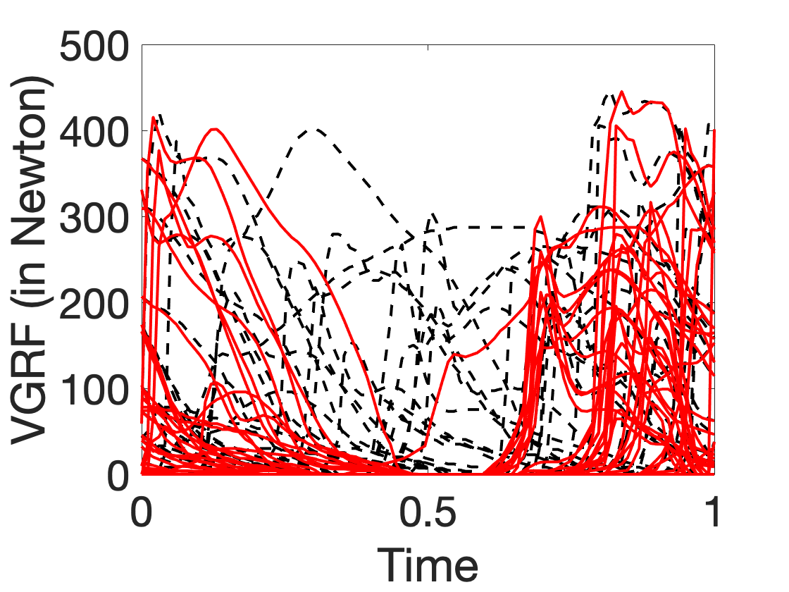


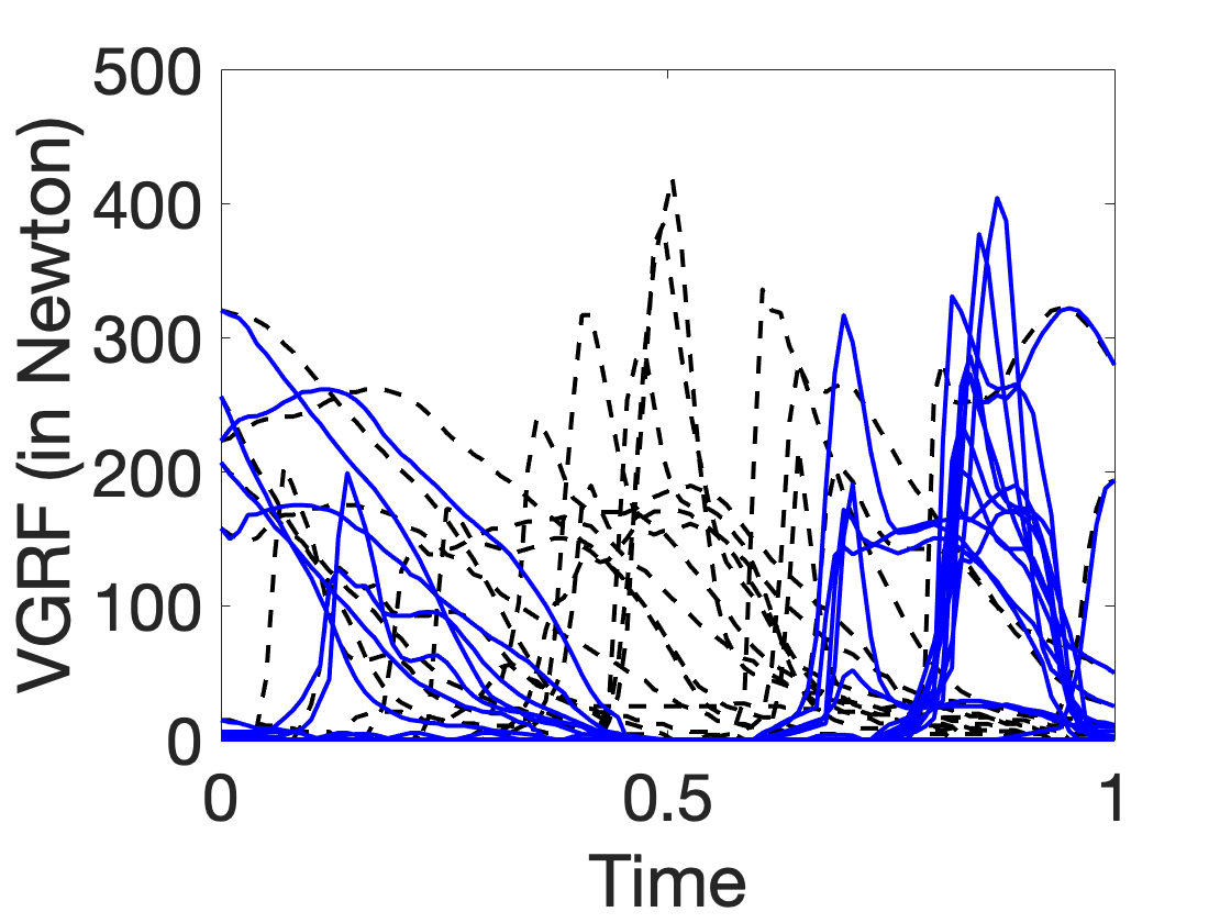


Fig. 8 shows “aligned" functional predictors during training and testing. Each row corresponds to a real data set – gait in Parkinson’s disease (first row), metabonomic 1H-NMR (second row), and historical stock market (third row). The original functions are drawn in black dashed curves and the warped functions are overlaid using the red/blue solid colors. Fig. 8(a) and 8(b) show the curves for the training data and the test data, respectively. The corresponding optimal warpings for training and test are shown in Fig. 8(c) and 8(d), respectively. We remind the readers that the predictors have been warped using the norm-preserving action during the optimization step. They appear more aligned than before but are not as aligned as one would get from a pure alignment procedure. This alignment results in an increased ability of the model to predict the response variable. Thus, this warping is more to help regress the responses s to the predictors s, rather than to align peaks and valleys in s.
Prediction Results
Table 4 presents prediction RMSE for different models studied in this experiment. It shows that EFRM model outperforms other models on all three datasets. In the case of 1H-NMR data, EFRM using a cubic index function does the best, while in other cases lower order polynomials perform better. This could be because the response variable in NMR example is categorical with four values and one needs a cubic polynomial to fit these response levels. Predictions from the kernel regression model are close second to EFRM.
| Model | Gait | 1H-NMR | Stock |
|---|---|---|---|
| : Linear | 2.741 | 4.849 | 9.007 |
| : Quadratic | 2.466 | 4.106 | 9.130 |
| : Cubic | 2.594 | 4.025 | 9.227 |
| FLM | 7.483 | 213.490 | 10.405 |
| PAFLM | 19.158 | 202.941 | 11.086 |
| NP- | 6.559 | 4.251 | 9.795 |
| NP-shape | 2.625 | 4.251 | 9.540 |
4 Concluding Remarks
The development of functional regression models that can handle phase variability in functional predictors is a challenging problem in FDA. We have proposed a new elastic approach that uses the shapes of functions, rather than the full functions, as predictors in regression models. The notion of shape is based on a norm-preserving warping of the predictors and handles the nuisance phase variability by optimizing the inner product over the warping group inside the model. We compare the prediction RMSE of the model with several existing methods, to demonstrate effectiveness of this technique in both simulated data and real data.
As discussed in Section 1.3, there is another model that can potentially eliminate the effects of phase variability in the predictor functional data. This model involves SRVFs of the predictors and uses the term as the argument of the index function . However, we have not pursued this model because, despite theoretical advantages, the practical performances of this model are sometimes low. As an example, we study the prediction problem using the same stock market data as in item 3 of Section 3.2. The prediction RMSE for this model is listed in Table 5, and is found to be worse than the results shown in Table 4. We conjecture that it is because the noise in predictor data gets enhanced when computing SRVFs (due to the presence of a time derivative in SRVF expression). Thus, we prefer the second option mentioned in Section 1.3 for EFRM.
| Model | : Linear | : Quadratic | : Cubic |
|---|---|---|---|
| RMSE | 18.032 | 18.139 | 18.110 |
Acknowledgement
This research was supported in part by the NSF grants NSF-1621787 and NSF-1617397 to AS. This paper describes objective technical results and analysis. Any subjective views or opinions that might be expressed in the paper do not necessarily represent the views of the U.S. Department of Energy or the United States Government. Supported by the Laboratory Directed Research and Development program at Sandia National Laboratories, a multi-mission laboratory managed and operated by National Technology and Engineering Solutions of Sandia, LLC, a wholly owned subsidiary of Honeywell International, Inc., for the U.S. Department of Energy’s National Nuclear Security Administration under contract DE-NA0003525.
Availability
MATLAB programs are available on Github: https://github.com/fdastat/elastic-regression
References
References
- [1] J. O. Ramsay, B. W. Silverman, Functional Data Analysis, 2nd Edition, Springer, 2005. doi:10.1007/b98888.
- [2] J. S. Morris, Functional regression, Annual Review of Statistics and Its Application 2 (2015) 321–359. doi:10.1146/annurev-statistics-010814-020413.
- [3] J. O. Ramsay, C. J. Dalzell, Some Tools for Functional Data Analysis, Journal of the Royal Statistical Society. Series B (Methodological) 53 (3) (1991) 539–572. doi:10.1111/j.2517-6161.1991.tb01844.x.
- [4] H. Cardot, F. Ferraty, P. Sarda, Functional linear model, Statistics & Probability Letters 45 (1) (1999) 11–22. doi:10.1016/s0167-7152(99)00036-x.
- [5] K. Ahn, J. D. Tucker, W. Wu, A. Srivastava, Elastic Handling of Predictor Phase in Functional Regression Models, in: Proceedings of the IEEE Conference on Computer Vision and Pattern Recognition Workshops, 2018, pp. 324–331. doi:10.1109/cvprw.2018.00072.
- [6] G. M. James, Generalized Linear Models with Functional Predictors, Journal of the Royal Statistical Society. Series B (Statistical Methodology) 64 (3) (2002) 411–432. doi:10.1111/1467-9868.00342.
- [7] P. T. Reiss, J. Goldsmith, H. L. Shang, R. T. Ogden, Methods for Scalar-on-Function Regression, International Statistical Review 85 (2) (2017) 228–249. doi:10.1111/insr.12163.
- [8] J. Goldsmith, F. Scheipl, Estimator selection and combination in scalar-on-function regression, Computational Statistics & Data Analysis 70 (2014) 362–372. doi:10.1016/j.csda.2013.10.009.
- [9] K. Fuchs, F. Scheipl, S. Greven, Penalized scalar-on-functions regression with interaction term, Computational Statistics & Data Analysis 81 (2015) 38–51. doi:10.1016/j.csda.2014.07.001.
- [10] A. Ciarleglio, R. T. Ogden, Wavelet-based scalar-on-function finite mixture regression models, Computational Statistics & Data Analysis 93 (2016) 86–96. doi:10.1016/j.csda.2014.11.017.
- [11] J. Gertheiss, J. Goldsmith, C. Crainiceanu, S. Greven, Longitudinal scalar-on-functions regression with application to tractography data, Biostatistics 14 (3) (2013) 447–461. doi:10.1093/biostatistics/kxs051.
- [12] T. T. Cai, P. Hall, Prediction in functional linear regression, The Annals of Statistics 34 (5) (2006) 2159–2179. doi:10.1214/009053606000000830.
- [13] H. G. Müller, U. Stadtmüller, Generalized functional linear models, The Annals of Statistics (2005) 774–805doi:10.1214/009053604000001156.
- [14] J. S. Marron, J. O. Ramsay, L. M. Sangalli, A. Srivastava, Functional data analysis of amplitude and phase variation, Statistical Science 30 (4) (2015) 468–484. doi:10.1214/15-sts524.
- [15] J. S. Marron, J. O. Ramsay, L. M. Sangalli, A. Srivastava, Statistics of time warpings and phase variations, Electronic Journal of Statistics 8 (2) (2014) 1697–1702. doi:10.1214/14-ejs901.
- [16] A. Srivastava, W. Wu, S. Kurtek, E. Klassen, J. S. Marron, Registration of Functional Data Using Fisher-Rao Metric arXiv:1103.3817.
- [17] J. D. Tucker, W. Wu, A. Srivastava, Generative Models for Functional Data Using Phase and Amplitude Separation, Computational Statistics & Data Analysis 61 (2013) 50–66. doi:10.1016/j.csda.2012.12.001.
- [18] M. Febrero-Bande, M. Oviedo de la Fuente, Statistical computing in functional data analysis: the R package fda. usc, Journal of Statistical Software 51 (4) (2012) 1–28. doi:10.18637/jss.v051.i04.
- [19] E. García-Portugués, W. González-Manteiga, M. Febrero-Bande, A goodness-of-fit test for the functional linear model with scalar response, Journal of Computational and Graphical Statistics 23 (3) (2014) 761–778. doi:10.1080/10618600.2013.812519.
- [20] J. O. Ramsay, X. Li, Curve Registration, Journal of the Royal Statistical Society: Series B (Statistical Methodology 60 (1998) 351–363. doi:10.1111/1467-9868.00129.
- [21] X. Liu, H. G. Müller, Functional convex averaging and synchronization for time-warped random curves, Journal of the American Statistical Association 99 (2004) 687–699. doi:10.1198/016214504000000999.
- [22] A. Srivastava, E. Klassen, Functional and shape data analysis, Springer, 2016. doi:10.1007/978-1-4939-4020-2.
- [23] F. Ferraty, P. Vieu, Nonparametric functional data analysis: theory and practice, Springer Science & Business Media, 2006. doi:10.1007/0-387-36620-2.
- [24] E. A. Nadaraya, On estimating regression, Theory of Probability & Its Applications 9 (1) (1964) 141–142. doi:10.1137/1109020.
- [25] T. M. Stoker, Consistent estimation of scaled coefficients, Econometrica: Journal of the Econometric Society (1986) 1461–1481doi:10.2307/1914309.
- [26] A. Ait-Saïdi, F. Ferraty, R. Kassa, P. Vieu, Cross-validated estimations in the single-functional index model, Statistics 42 (6) (2008) 475–494. doi:10.1080/02331880801980377.
- [27] P. H. C. Eilers, B. D. Marx, Flexible Smoothing with B-Splines and Penalties, Statistical Science (1996) 89–102doi:10.1214/ss/1038425655.
- [28] C. R. Jiang, J. L. Wang, Functional single index models for longitudinal data, The Annals of Statistics 39 (1) (2011) 362–388. doi:10.1214/10-AOS845.
- [29] P. H. C. Eilers, B. Li, B. D. Marx, Multivariate calibration with single-index signal regression, Chemometrics and Intelligent Laboratory Systems 96 (2) (2009) 196–202. doi:10.1016/j.chemolab.2009.02.001.
- [30] Y. Li, N. Wang, R. J. Carroll, Generalized functional linear models with semiparametric single-index interactions, Journal of the American Statistical Association 105 (490) (2010) 621–633. doi:10.1198/jasa.2010.tm09313.
- [31] J. S. Morris, Functional regression, Annual Review of Statistics and Its Application 2 (2015) 321–359. doi:10.1146/annurev-statistics-010814-020413.
- [32] A. L. Goldberger, L. A. N. Amaral, L. Glass, J. M. Hausdorff, P. C. Ivanov, R. G. Mark, J. E. Mietus, G. B. Moody, C. Peng, H. E. Stanley, PhysioBank, PhysioToolkit, and PhysioNet: Components of a New Research Resource for Complex Physiologic Signals, Circulation 101 (23) (2000) e215–e220. doi:10.1161/01.cir.101.23.e215.
- [33] S. Frenkel-Toledo, N. Giladi, C. Peretz, T. Herman, L. Gruendlinger, J. M. Hausdorff, Treadmill walking as an external pacemaker to improve gait rhythm and stability in Parkinson’s disease, Movement Disorders 20 (9) (2005) 1109–1114. doi:10.1002/mds.20507.
- [34] S. Frenkel-Toledo, N. Giladi, C. Peretz, T. Herman, L. Gruendlinger, J. M. Hausdorff, Effect of gait speed on gait rhythmicity in Parkinson’s disease: variability of stride time and swing time respond differently, Journal of NeuroEngineering and Rehabilitation 2 (1) (2005) 23. doi:10.1186/1743-0003-2-23.
- [35] G. Yogev, N. Giladi, C. Peretz, S. l. Springer, E. S. Simon, J. M. Hausdorff, Dual tasking, gait rhythmicity, and Parkinson’s disease: which aspects of gait are attention demanding?, European Journal of Neuroscience 22 (5) (2005) 1248–1256. doi:10.1111/j.1460-9568.2005.04298.x.
- [36] H. Winning, E. Roldán-Marín, L. O. Dragsted, N. Viereck, M. Poulsen, C. Sánchez-Moreno, M. P. Cano, S. Engelsen, An exploratory NMR nutri-metabonomic investigation reveals dimethyl sulfone as a dietary biomarker for onion intake, Analyst 134 (11) (2009) 2344–2351. doi:10.1039/b918259d.