跳到论文正文
W Papers独立论文阅读器 arXiv:1909.02278 论文正文 计算阅读时间 · 0%
引用这篇论文根据当前论文元数据生成,正式投稿前建议核对。


License: arXiv.org perpetual non-exclusive license
arXiv:1909.02278v2 [math.CO] 27 Mar 2020

Integrability approach to Fehér-Némethi-Rimányi-Guo-Sun type identities for factorial Grothendieck polynomials

Kohei Motegi Thanks: E-mail: kmoteg0@kaiyodai.ac.jp Affiliation: Faculty of Marine Technology, Tokyo University of Marine Science and Technology, Affiliation: Etchujima 2-1-6, Koto-Ku, Tokyo, 135-8533, Japan
August 11, 2026
Abstract

Recently, Guo and Sun derived an identity for factorial Grothendieck polynomials which is a generalization of the one for Schur polynomials by Fehér, Némethi and Rimányi. We analyze the identity from the point of view of quantum integrability, based on the correspondence between the wavefunctions of a five-vertex model and the Grothendieck polynomials. We give another proof using the quantum inverse scattering method. We also apply the same idea and technique to derive an identity for factorial Grothendieck polynomials for rectangular Young diagrams. Combining with the Guo-Sun identity, we get a duality formula. We also discuss a qq-deformation of the Guo-Sun identity.

1 Introduction

Recently, Guo and Sun derived identities for factorial Grothendieck polynomials [1]. The factorial β\beta-Grothendieck polynomials, which is a KK-theoretic analogue of the factorial Schur polynomials [2, 3, 4, 5], have the following determinant form [6, 7]

Gλ​(𝒛|𝜶)=detn​([zi|𝜶]λj+n−j​(1+β​zi)j−1)∏1≤i<j≤n(zi−zj),\displaystyle G_{\lambda}(\boldsymbol{z}|\boldsymbol{\alpha})=\frac{\mathrm{det}_{n}([z_{i}|\boldsymbol{\alpha}]^{\lambda_{j}+n-j}(1+\beta z_{i})^{j-1})}{\prod_{1\leq i<j\leq n}(z_{i}-z_{j})}, (1.1)

where λ=(λ1,λ2,…,λn)\lambda=(\lambda_{1},\lambda_{2},\dots,\lambda_{n}) is a partition, i.e. a nonincreasing sequence of nonnegative integers whose graphical representation is naturally given by the Young diagram. 𝒛={z1,…,zn}\boldsymbol{z}=\{z_{1},\dots,z_{n}\} is a set of symmetric variables, 𝜶={α1,α2,…}\boldsymbol{\alpha}=\{\alpha_{1},\alpha_{2},\dots\} is a set of factorial variables and

[zi|𝜶]j=(zi⊕α1)(zi⊕α2)⋯(zi⊕αj),\displaystyle[z_{i}|\boldsymbol{\alpha}]^{j}=(z_{i}\oplus\alpha_{1})(z_{i}\oplus\alpha_{2})\cdots(z_{i}\oplus\alpha_{j}), (1.2)

where z⊕α:=z+α+β​z​αz\oplus\alpha:=z+\alpha+\beta z\alpha.

One of the identities Guo and Sun derived is the following one [1]: for a partition λ=(λ,…,λk)\lambda=(\lambda,\dots,\lambda_{k}) such that λ1≤m−k\lambda_{1}\leq m-k and another one μ=((m−k)n−k,λ1,…,λk)\mu=((m-k)^{n-k},\lambda_{1},\dots,\lambda_{k}), the following identity holds:

Gμ​(𝒛|𝜶)=∑Skn∈([n]k)Gλ​(𝒛Skn|𝜶)​∏i∈Skn(1+β​zi)n−k​∏j∈Skn¯[zj|𝜶]m∏i∈Skn∏j∈Skn¯(zj−zi),\displaystyle G_{\mu}(\boldsymbol{z}|\boldsymbol{\alpha})=\sum_{S_{k}^{n}\in\binom{[n]}{k}}G_{\lambda}(\boldsymbol{z}_{S_{k}^{n}}|\boldsymbol{\alpha})\frac{\displaystyle\prod_{i\in{S_{k}^{n}}}(1+\beta z_{i})^{n-k}\prod_{j\in\overline{S_{k}^{n}}}[z_{j}|\boldsymbol{\alpha}]^{m}}{\displaystyle\prod_{i\in{S_{k}^{n}}}\prod_{j\in\overline{{S_{k}^{n}}}}(z_{j}-z_{i})}, (1.3)

where SknS_{k}^{n} is a kk-subset of [n]={1,2,…,n}[n]=\{1,2,\dots,n\}, ([n]k)\binom{[n]}{k} is the set of kk-subsets of nn, Skn¯={1,2,…,n}\Skn\overline{S_{k}^{n}}=\{1,2,\dots,n\}\backslash S_{k}^{n}, and Gλ​(𝒛Skn|𝜶)=Gλ​({zi1,…,zik}|𝜶)G_{\lambda}(\boldsymbol{z}_{S_{k}^{n}}|\boldsymbol{\alpha})=G_{\lambda}(\{z_{i_{1}},\dots,z_{i_{k}}\}|\boldsymbol{\alpha}) for Skn={i1,…,ik}S_{k}^{n}=\{i_{1},\dots,i_{k}\}.

This identity generalizes the one for the Schur polynomials derived by Fehér, Némethi and Rimányi [8] which corresponds to the case β=α1=α2=⋯=0\beta=\alpha_{1}=\alpha_{2}=\dots=0, and we will call this type of identity as Fehér-Némethi-Rimányi-Guo-Sun type identity.

In this paper, we restrict to the case β=−1\beta=-1, and investigate this identity and also derive similar identities from the viewpoint of quantum integrability. Recently, there is an active line of research which investigates relations between integrable models and related structures (integrable lattice models, classical integrable systems, vertex operators, crystal basis) and the (dual, symmetric) Grothendieck polynomials, and study the properties of the Grothendieck polynomials using the connections. See [9, 10, 11, 12, 13, 14, 15, 16, 17] for examples for various topics. We give another proof of the Guo-Sun identity (1.3) using the quantum inverse scattering method [18, 19], which is a method developed to study quantum integrable models. Why we can use this method for giving another proof is based on the correspondence between certain types of partition functions of an integrable five-vertex model and the Grothendieck polynomials. This correspondence was used to investigate Cauchy-type identities, Gromov-Witten invariants and Littlewood-Richardson coefficients [9, 10, 12, 13]. In this paper, we give another application of the correspondence. Namely, we give an integrability proof of the Guo-Sun identity using the quantum inverse scattering method. We also apply the same idea and technique to derive an identity for factorial Grothendieck polynomials for rectangular Young diagrams. The five-vertex model which is used can be regarded as a certain limit of the Uq​(s​l2^)U_{q}(\widehat{sl_{2}}) six-vertex model [20, 21, 22]. Based on this viewpoint, we also discuss a qq-deformation by following the line of computation to derive the Guo-Sun identity.

This paper is organized as follows. In the next section, we explain the correspondence between the wavefunctions of the Uq​(s​l2^)U_{q}(\widehat{sl_{2}}) six-vertex model and symmetric functions, and its q=0q=0 degeneration which gives the correspondence between the wavefunctions of the five-vertex model and the factorial Grothendieck polynomials. In section 3, we give another proof of the Guo-Sun identity by using the quantum inverse scattering method. In section 4, we derive an identity for the factorial Grothendieck polynomials for rectangular shapes by using the same idea and technique in section 3 to “a different direction”. We discuss a qq-deformation of the Guo-Sun identity by applying the same idea to the Uq​(s​l2^)U_{q}(\widehat{sl_{2}}) six-vertex model. Section 5 is devoted to the conclusion of this paper.

2 Uq​(s​l2^)U_{q}(\widehat{sl_{2}}) six-vertex model, wavefunctions and degeneration to the five-vertex model

In this section, we first introduce the Uq​(s​l2^)U_{q}(\widehat{sl_{2}}) six-vertex model and explain the correspondence between the wavefunctions and symmetric functions. Next, we degenerate the six-vertex model to the five-vertex model and explain the correspondence between the wavefunctions and the factorial Grothendieck polynomials.

The Uq​(s​l2^)U_{q}(\widehat{sl_{2}}) RR-matrix is the following matrix [20, 21] (Figure 1)

Ra​b​(u,w)=(u−q​w0000q⁡(u−w)(1−q)​u00(1−q)​wu−w0000u−q​w),\displaystyle R_{ab}(u,w)=\left(\begin{array}[]{cccc}u-qw&0&0&0\\ 0&q(u-w)&(1-q)u&0\\ 0&(1-q)w&u-w&0\\ 0&0&0&u-qw\end{array}\right),

acting on the tensor product Wa⊗WbW_{a}\otimes W_{b} of the complex two-dimensional space WaW_{a}. We denote the dual space of WaW_{a} by Wa∗W_{a}^{*}.

Refer to caption
Figure 1: The RR-matrix of the six-vertex model (2). There are six admissible vertex configurations, and the weight associated to each configuration is given below the figure of the configuration.

The RR-matrix (2) satisifies the Yang-Baxter relation

Ra​b​(u,v)​Ra​c​(u,w)​Rb​c​(v,w)=Rb​c​(v,w)​Ra​c​(u,w)​Ra​b​(u,v),\displaystyle R_{ab}(u,v)R_{ac}(u,w)R_{bc}(v,w)=R_{bc}(v,w)R_{ac}(u,w)R_{ab}(u,v), (2.6)

acting on Wa⊗Wb⊗WcW_{a}\otimes W_{b}\otimes W_{c}.

We denote the orthonormal basis of WaW_{a} and its dual as {|0⟩a,|1⟩a}\{|0\rangle_{a},|1\rangle_{a}\} and {⟨0|,⟨1|}aa\{{}_{a}\langle 0|,{}_{a}\langle 1|\}. We also introduce the following Pauli spin operators σ+\sigma^{+} and σ−\sigma^{-} as operators acting on the (dual) orthonomal basis as

σ+​|1⟩=|0⟩,σ+​|0⟩=0,⟨0|​σ+=⟨1|,⟨1|​σ+=0,\displaystyle\sigma^{+}|1\rangle=|0\rangle,\ \sigma^{+}|0\rangle=0,\ \langle 0|\sigma^{+}=\langle 1|,\ \langle 1|\sigma^{+}=0, (2.7)
σ−​|0⟩=|1⟩,σ−​|1⟩=0,⟨1|​σ−=⟨0|,⟨0|​σ−=0.\displaystyle\sigma^{-}|0\rangle=|1\rangle,\ \sigma^{-}|1\rangle=0,\ \langle 1|\sigma^{-}=\langle 0|,\ \langle 0|\sigma^{-}=0. (2.8)

The monodromy matrix Ta​(u|w1,…,wm+n−k)T_{a}(u|w_{1},\dots,w_{m+n-k}) is the product of RR-matrices

Ta​(u|w1,…,wm+n−k)\displaystyle T_{a}(u|w_{1},\dots,w_{m+n-k}) =Ra,m+n−k(u,wm+n−k)⋯Ra​1(u,w1)\displaystyle=R_{a,m+n-k}(u,w_{m+n-k})\cdots R_{a1}(u,w_{1})
=(A⁡(u|w1,…,wm+n−k)B⁡(u|w1,…,wm+n−k)C⁡(u|w1,…,wm+n−k)D⁡(u|w1,…,wm+n−k))a,\displaystyle=\begin{pmatrix}A(u|w_{1},\dots,w_{m+n-k})&B(u|w_{1},\dots,w_{m+n-k})\\ C(u|w_{1},\dots,w_{m+n-k})&D(u|w_{1},\dots,w_{m+n-k})\end{pmatrix}_{a}, (2.9)

acting on Wa⊗W1⊗⋯⊗Wm+n−kW_{a}\otimes W_{1}\otimes\cdots\otimes W_{m+n-k}.

The BB-operator is a matrix element of the monodromy matrix Ta​(u|w1,…,wm+n−k)T_{a}(u|w_{1},\dots,w_{m+n-k})

B(u|w1,…,wm+n−k)=⟨0|Ta(u|w1,…,wm+n−k)|1⟩aa,\displaystyle B(u|w_{1},\dots,w_{m+n-k})={}_{a}\langle 0|T_{a}(u|w_{1},\dots,w_{m+n-k})|1\rangle_{a}, (2.10)

acting on W1⊗⋯⊗Wm+n−kW_{1}\otimes\cdots\otimes W_{m+n-k}.

Let us define the (dual) vacuum state as |Ω⟩m+n−k:=|0⟩1⊗⋯⊗|0⟩m+n−k∈W1⊗⋯⊗Wm+n−k|\Omega\rangle_{m+n-k}:=|0\rangle_{1}\otimes\cdots\otimes|0\rangle_{m+n-k}\in W_{1}\otimes\cdots\otimes W_{m+n-k} ( ⟨Ω|:=⟨0|⊗⋯⊗⟨0|∈W1∗⊗⋯⊗Wm+n−k∗m+n−k1m+n−k{}_{m+n-k}\langle\Omega|:={}_{1}\langle 0|\otimes\cdots\otimes{}_{m+n-k}\langle 0|\in W_{1}^{*}\otimes\cdots\otimes W_{m+n-k}^{*}) and configuration vectors as

⟨x1⋯xn|m+n−k{}_{m+n-k}\langle x_{1}\cdots x_{n}| =⟨Ω|∏j=1nσxj+∈W1∗⊗⋯⊗Wm+n−k∗,m+n−k\displaystyle={}_{m+n-k}\langle\Omega|\prod_{j=1}^{n}\sigma^{+}_{x_{j}}\in W_{1}^{*}\otimes\cdots\otimes W_{m+n-k}^{*}, (2.11)

for 1≤x1<x2<⋯<xn≤m+n−k1\leq x_{1}<x_{2}<\cdots<x_{n}\leq m+n-k.

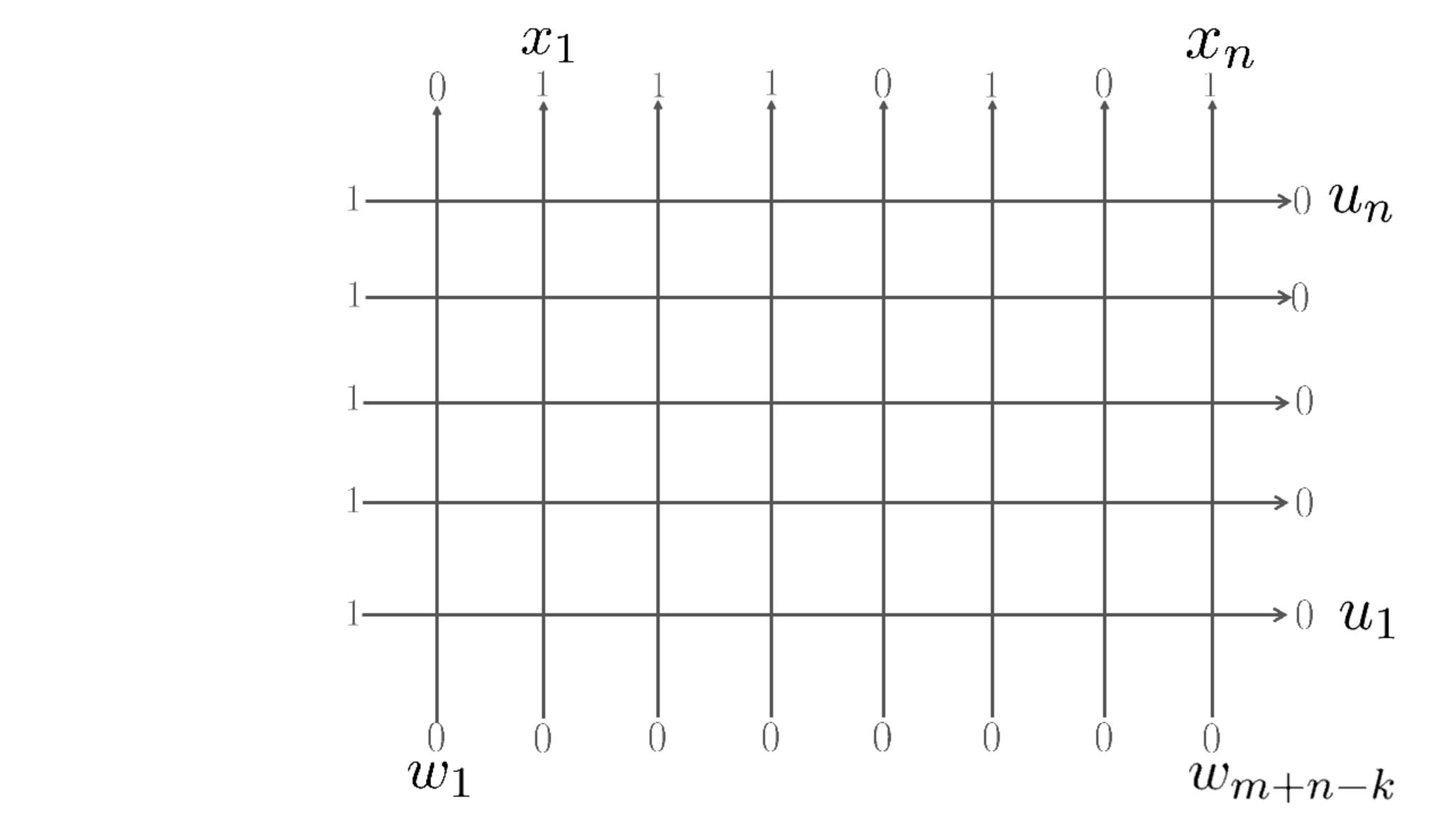
We now introduce the wavefunctions Wm+n−k,n(u1,…,un|w1,…,wm+n−k|x1,…,xn)W_{m+n-k,n}(u_{1},\dots,u_{n}|w_{1},\dots,w_{m+n-k}|x_{1},\dots,x_{n}) as (Figure 2)

Wm+n−k,n(u1,…,un|w1,…,wm+n−k|x1,…,xn)\displaystyle W_{m+n-k,n}(u_{1},\dots,u_{n}|w_{1},\dots,w_{m+n-k}|x_{1},\dots,x_{n})
=\displaystyle= ⟨x1⋯xn|B(un|w1,…,wm+n−k)⋯B(u1|w1,…,wm+n−k)|Ω⟩m+n−km+n−k.{}_{m+n-k}\langle x_{1}\cdots x_{n}|B(u_{n}|w_{1},\dots,w_{m+n-k})\cdots B(u_{1}|w_{1},\dots,w_{m+n-k})|\Omega\rangle_{m+n-k}. (2.12)
Refer to caption
Figure 2: The wavefunctions (2.12). The sequence of 0s on the bottom part represents the vacuum state |Ω⟩m+n−k|\Omega\rangle_{m+n-k}. The jj-th row counted from the bottom represents the BB-operator B⁡(uj|w1,…,wm+n−k)B(u_{j}|w_{1},\dots,w_{m+n-k}) and the top part which is a sequence of 0s and 1s represents the dual vector ⟨x1⋯xn|m+n−k{}_{m+n-k}\langle x_{1}\cdots x_{n}|. The dual vector is labelled by the positions x1,…,xnx_{1},\dots,x_{n} of 1s counted from the left. The figure illustrates the case n=5n=5, m=k+3m=k+3, (x1,x2,x3,x4,x5)=(2,3,4,6,8)(x_{1},x_{2},x_{3},x_{4},x_{5})=(2,3,4,6,8).

We next define the following symmetric function
Fm+n−k,n(u1,…,un|w1,…,wm+n−k|x1,…,xn)F_{m+n-k,n}(u_{1},\dots,u_{n}|w_{1},\dots,w_{m+n-k}|x_{1},\dots,x_{n}) which depends on the symmetric variables u1,…,unu_{1},\dots,u_{n}, complex parameters w1,…,wm+n−kw_{1},\dots,w_{m+n-k} and integers x1,…,xnx_{1},\dots,x_{n} satisfying 1≤x1<⋯<xn≤m+n−k1\leq x_{1}<\cdots<x_{n}\leq m+n-k,

Fm+n−k,n(u1,…,un|w1,…,wm+n−k|x1,…,xn)\displaystyle F_{m+n-k,n}(u_{1},\dots,u_{n}|w_{1},\dots,w_{m+n-k}|x_{1},\dots,x_{n})
=\displaystyle= ∑σ∈Sn∏j=1n∏i=xj+1m+n−k(uσ⁡(j)−q​wi)​∏1≤i<j≤nq​uσ⁡(i)−uσ⁡(j)uσ⁡(i)−uσ⁡(j)\displaystyle\sum_{\sigma\in S_{n}}\prod_{j=1}^{n}\prod_{i=x_{j}+1}^{m+n-k}(u_{\sigma(j)}-qw_{i})\prod_{1\leq i<j\leq n}\frac{qu_{\sigma(i)}-u_{\sigma(j)}}{u_{\sigma(i)}-u_{\sigma(j)}}
×∏j=1n∏i=1xj−1(uσ⁡(j)−wi)​∏j=1n(1−q)​uσ⁡(j).\displaystyle\times\prod_{j=1}^{n}\prod_{i=1}^{x_{j}-1}(u_{\sigma(j)}-w_{i})\prod_{j=1}^{n}(1-q)u_{\sigma(j)}. (2.13)

The wavefunction Wm+n−k,n(u1,…,un|w1,…,wm+n−k|x1,…,xn)W_{m+n-k,n}(u_{1},\dots,u_{n}|w_{1},\dots,w_{m+n-k}|x_{1},\dots,x_{n}) is explicitly expressed as the symmetric function Fm+n−k,n(u1,…,un|w1,…,wm+n−k|x1,…,xn)F_{m+n-k,n}(u_{1},\dots,u_{n}|w_{1},\dots,w_{m+n-k}|x_{1},\dots,x_{n})

Wm+n−k,n(u1,…,un|w1,…,wm+n−k|x1,…,xn)\displaystyle W_{m+n-k,n}(u_{1},\dots,u_{n}|w_{1},\dots,w_{m+n-k}|x_{1},\dots,x_{n})
=\displaystyle= Fm+n−k,n(u1,…,un|w1,…,wm+n−k|x1,…,xn).\displaystyle F_{m+n-k,n}(u_{1},\dots,u_{n}|w_{1},\dots,w_{m+n-k}|x_{1},\dots,x_{n}). (2.14)

See [23, 24] for example for proofs of this correspondence. Next, we explain the degeneration of the correspondence (2.14). If one sets qq to q=0q=0, the RR-matrix for the six-vertex model (2) reduces to that for the five-vertex model

Ra​b​(u,w)|q=0=(u00000u00wu−w0000u).\displaystyle R_{ab}(u,w)|_{q=0}=\left(\begin{array}[]{cccc}u&0&0&0\\ 0&0&u&0\\ 0&w&u-w&0\\ 0&0&0&u\end{array}\right).

Under the change of variables zj=1−uj−1​(j=1,…,n)z_{j}=1-u_{j}^{-1}\ (j=1,\dots,n), αj=1−wj​(j=1,…,m+n−k)\alpha_{j}=1-w_{j}\ (j=1,\dots,m+n-k), λj=xn−j+1−n+j−1​(j=1,…,n)\lambda_{j}=x_{n-j+1}-n+j-1\ (j=1,\dots,n), the correspondence at q=0q=0 (2.14) becomes the following correspondence between the wavefunctions of the five-vertex model and the β=−1\beta=-1 factorial Grothendieck polynomials [9, 10, 12, 13]

Wm+n−k,n(u1,…,un|w1,…,wm+n−k|x1,…,xn)|q=0\displaystyle W_{m+n-k,n}(u_{1},\dots,u_{n}|w_{1},\dots,w_{m+n-k}|x_{1},\dots,x_{n})|_{q=0}
=\displaystyle= ∏j=1n1(1−zj)m+n−k​Gλ​({z1,…,zn}|𝜶).\displaystyle\prod_{j=1}^{n}\frac{1}{(1-z_{j})^{m+n-k}}G_{\lambda}(\{z_{1},\dots,z_{n}\}|\boldsymbol{\alpha}). (2.20)

We use this correspondence in the next two sections to investigate identities for the factorial Grothendieck polynomials from the viewpoint of quantum integrability.

3 Integrability proof of Guo-Sun identity

In this and the next sections, we consider the five-vertex model whose RR-matrix is given by (2) which is the q=0q=0 limit of (2). Every object introduced in the last section should be understood that we set qq to q=0q=0 in this and the next sections.

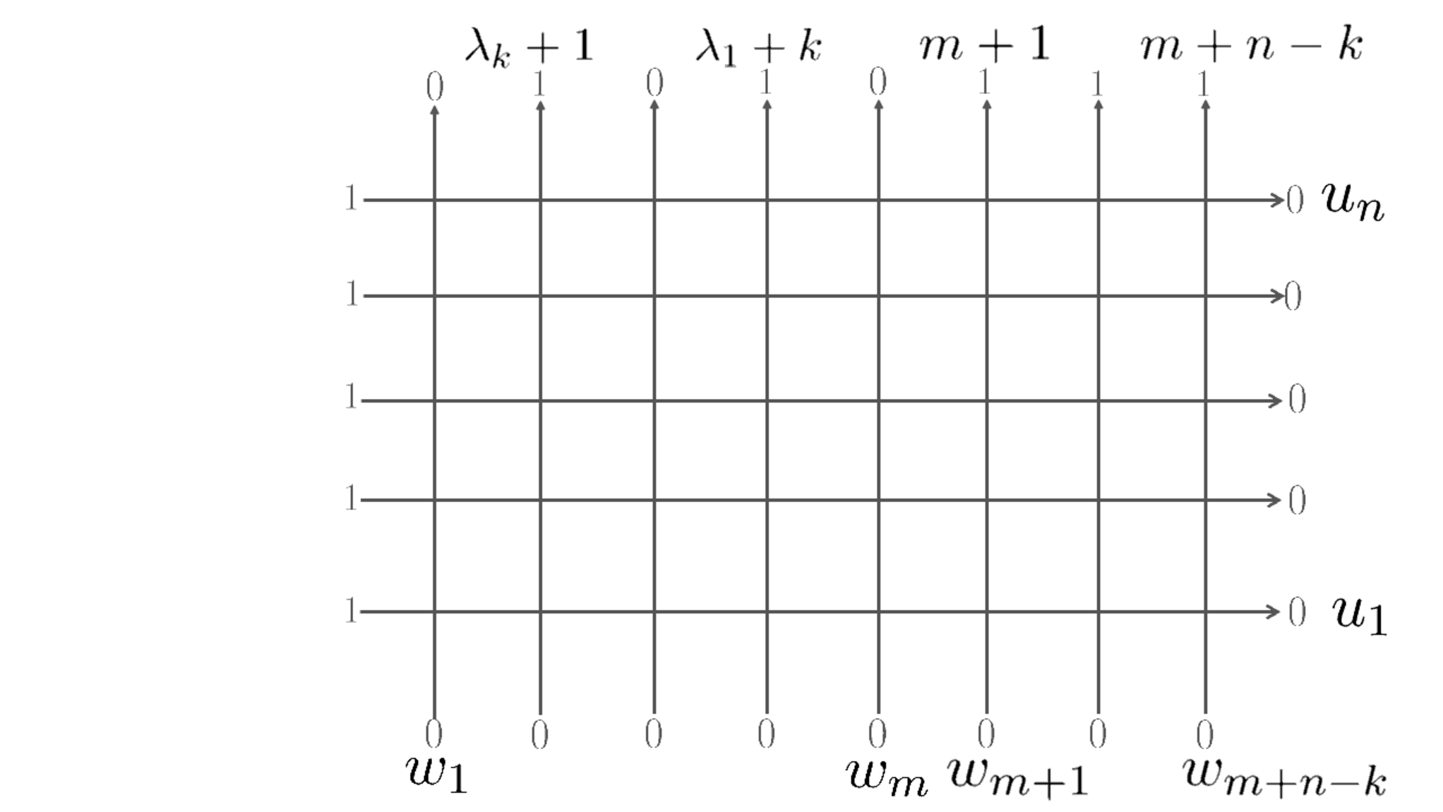
In this section, let us show another proof of Guo-Sun identity (1.3) using the quantum inverse scattering method. They derived an identity for Grothendieck polynomials of the following partition μ=((m−k)n−k,λ1,…,λk)\mu=((m-k)^{n-k},\lambda_{1},\dots,\lambda_{k}). Applying the correspondence (2.20) to this partition, we have

Wm+n−k,n(u1,…,un|w1,…,wm+n−k|λk+1,…,λ1+k,m+1,…,m+n−k)\displaystyle W_{m+n-k,n}(u_{1},\dots,u_{n}|w_{1},\dots,w_{m+n-k}|\lambda_{k}+1,\dots,\lambda_{1}+k,m+1,\dots,m+n-k)
=\displaystyle= ∏j=1n1(1−zj)m+n−k​Gμ​({z1,…,zn}|𝜶).\displaystyle\prod_{j=1}^{n}\frac{1}{(1-z_{j})^{m+n-k}}G_{\mu}(\{z_{1},\dots,z_{n}\}|\boldsymbol{\alpha}). (3.1)
Refer to caption
Figure 3: The wavefunctions corresponding to the factorial Grothendieck polynomials of partition μ=((m−k)n−k,λ1,…,λk)\mu=((m-k)^{n-k},\lambda_{1},\dots,\lambda_{k}) (3.1). The top part is a sequence of 0s and 1s. The 1s appear at positions λk+1\lambda_{k}+1, λk−1+2\lambda_{k-1}+2, …\dots, λ1+k\lambda_{1}+k, m+1m+1, m+2m+2, …\dots, m+n−km+n-k counted from the left. Subtracting 1,2,…,n1,2,\dots,n from λk+1\lambda_{k}+1, λk−1+2\lambda_{k-1}+2, …\dots, λ1+k\lambda_{1}+k, m+1m+1, m+2m+2, …\dots, m+n−km+n-k, and reorder as a nonincreasing sequence, we get the partition ((m−k)n−k,λ1,…,λk)((m-k)^{n-k},\lambda_{1},\dots,\lambda_{k}) which labels the sequence of 0s and 1s in this figure. The figure illustrates the case n=5n=5, m=5m=5, k=2k=2, (λ1,λ2)=(2,1)(\lambda_{1},\lambda_{2})=(2,1).

To prove the Guo-Sun identity, we investigate Wm+n−k,n(u1,…,un|w1,…,wm+n−k|λk+1,…,λ1+k,m+1,…,m+n−k)W_{m+n-k,n}(u_{1},\dots,u_{n}|w_{1},\dots,w_{m+n-k}|\lambda_{k}+1,\dots,\lambda_{1}+k,m+1,\dots,m+n-k) using its graphical description (Figure 3) and derive another expression.

Refer to caption
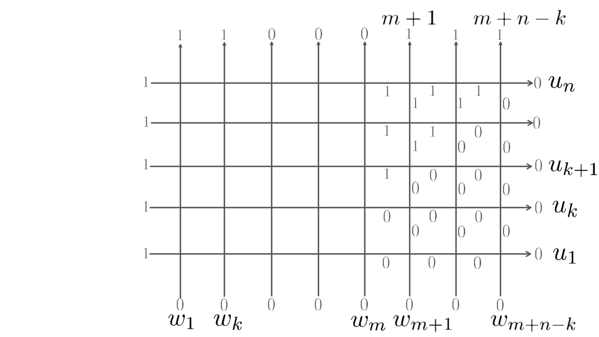
Figure 4: The wavefunction Wm+n−k,n(u1,…,un|w1,…,wm+n−k|λk+1,…,λ1+k,m+1,…,m+n−k)W_{m+n-k,n}(u_{1},\dots,u_{n}|w_{1},\dots,w_{m+n-k}|\lambda_{k}+1,\dots,\lambda_{1}+k,m+1,\dots,m+n-k). We can see that only one configuration is allowed in the rightmost n−kn-k columns, which gives the factor ∏j=1nujn−k\displaystyle\prod_{j=1}^{n}u_{j}^{n-k}. The remaining part can be expressed as ⟨λk+1,…,λ1+k|∏j=k+1nD(uj|w1,…,wm)∏j=1kB(uj|w1,…,wm)|Ω⟩mm\displaystyle{}_{m}\langle\lambda_{k}+1,\dots,\lambda_{1}+k|\prod_{j=k+1}^{n}D(u_{j}|w_{1},\dots,w_{m})\prod_{j=1}^{k}B(u_{j}|w_{1},\dots,w_{m})|\Omega\rangle_{m}.

First, from the graphical representation of Wm+n−k,n(u1,…,un|w1,…,wm+n−k|λk+1,…,λ1+k,m+1,…,m+n−k)W_{m+n-k,n}(u_{1},\dots,u_{n}|w_{1},\dots,w_{m+n-k}|\lambda_{k}+1,\dots,\lambda_{1}+k,m+1,\dots,m+n-k) and noting that the bulk weights are given by the RR-matrix of the five-vertex model (2), one can see that only one configuration is allowed in the rightmost n−kn-k columns (Figure 4), and we get the factor ∏j=1nujn−k\displaystyle\prod_{j=1}^{n}u_{j}^{n-k} from that configuration. Next, looking at the remaining part, we find that they are expressed as ⟨λk+1,…,λ1+k|∏j=k+1nD(uj|w1,…,wm)∏j=1kB(uj|w1,…,wm)|Ω⟩mm\displaystyle{}_{m}\langle\lambda_{k}+1,\dots,\lambda_{1}+k|\prod_{j=k+1}^{n}D(u_{j}|w_{1},\dots,w_{m})\prod_{j=1}^{k}B(u_{j}|w_{1},\dots,w_{m})|\Omega\rangle_{m}. Hence we have

Wm+n−k,n(u1,…,un|w1,…,wm+n−k|λk+1,…,λ1+k,m+1,…,m+n−k)\displaystyle W_{m+n-k,n}(u_{1},\dots,u_{n}|w_{1},\dots,w_{m+n-k}|\lambda_{k}+1,\dots,\lambda_{1}+k,m+1,\dots,m+n-k)
=\displaystyle= ∏j=1nujn−k⟨λk+1,…,λ1+k|∏j=k+1nD(uj|w1,…,wm)∏j=1kB(uj|w1,…,wm)|Ω⟩mm.\displaystyle\prod_{j=1}^{n}u_{j}^{n-k}{}_{m}\langle\lambda_{k}+1,\dots,\lambda_{1}+k|\prod_{j=k+1}^{n}D(u_{j}|w_{1},\dots,w_{m})\prod_{j=1}^{k}B(u_{j}|w_{1},\dots,w_{m})|\Omega\rangle_{m}. (3.2)

Next, we commute the multiple operators ∏j=k+1nD⁡(uj|w1,…,wm)\prod_{j=k+1}^{n}D(u_{j}|w_{1},\dots,w_{m}) with the multiple operators ∏j=1kB⁡(uj|w1,…,wm)\prod_{j=1}^{k}B(u_{j}|w_{1},\dots,w_{m}). From the Yang-Baxter relation (2.6), we get the intertwining relation for the monodromy matrices

Ra​b​(u1,u2)​Ta​(u1|w1,…,wm)​Tb​(u2|w1,…,wm)\displaystyle R_{ab}(u_{1},u_{2})T_{a}(u_{1}|w_{1},\dots,w_{m})T_{b}(u_{2}|w_{1},\dots,w_{m})
=\displaystyle= Tb​(u2|w1,…,wm)​Ta​(u1|w1,…,wm)​Ra​b​(u1,u2).\displaystyle T_{b}(u_{2}|w_{1},\dots,w_{m})T_{a}(u_{1}|w_{1},\dots,w_{m})R_{ab}(u_{1},u_{2}). (3.3)

Some matrix elements of (3.3) are given by

D⁡(u1)​B​(u2)\displaystyle D(u_{1})B(u_{2}) =u1u1−u2​B​(u2)​D​(u1)−u2u1−u2​B​(u1)​D​(u2),\displaystyle=\frac{u_{1}}{u_{1}-u_{2}}B(u_{2})D(u_{1})-\frac{u_{2}}{u_{1}-u_{2}}B(u_{1})D(u_{2}), (3.4)
D⁡(u1)​B​(u2)\displaystyle D(u_{1})B(u_{2}) =D⁡(u2)​B​(u1),\displaystyle=D(u_{2})B(u_{1}), (3.5)
B⁡(u1)​B​(u2)\displaystyle B(u_{1})B(u_{2}) =B⁡(u2)​B​(u1),\displaystyle=B(u_{2})B(u_{1}), (3.6)
D⁡(u1)​D​(u2)\displaystyle D(u_{1})D(u_{2}) =D⁡(u2)​D​(u1).\displaystyle=D(u_{2})D(u_{1}). (3.7)

For integrable models which have the RR-matrix of the five-vertex model as an intertwiner, a compact formula between the commutation relations between multiple DD-operators and BB-operators can be derived from (3.4), (3.5), (3.6), (3.7), following the argument of [25] (they were analyzing the integrable phase model [26], but the type of the representation for the quantum space does not affect the argument). The result is given by

∏j=k+1nD⁡(uj|w1,…,wm)​∏j=1kB⁡(uj|w1,…,wm)\displaystyle\prod_{j=k+1}^{n}D(u_{j}|w_{1},\dots,w_{m})\prod_{j=1}^{k}B(u_{j}|w_{1},\dots,w_{m})
=\displaystyle= ∑Skn∈([n]k)∏i∈Skn,j∈Skn¯ujuj−ui​∏i∈SknB⁡(ui|w1,…,wm)​∏j∈Skn¯D⁡(uj|w1,…,wm).\displaystyle\sum_{S_{k}^{n}\in\binom{[n]}{k}}\prod_{i\in S_{k}^{n},j\in\overline{S_{k}^{n}}}\frac{u_{j}}{u_{j}-u_{i}}\prod_{i\in S_{k}^{n}}B(u_{i}|w_{1},\dots,w_{m})\prod_{j\in\overline{S_{k}^{n}}}D(u_{j}|w_{1},\dots,w_{m}). (3.8)

(3.8) can be shown as follows (see the Proof of Theorem 6.1 in [25]). First, using (3.4), (3.6) and (3.7) to move all the BB-operators to the left of all the DD-operators, one notes the operator part of all the terms which appear can be expressed as

∏i∈SknB⁡(ui|w1,…,wm)​∏j∈Skn¯D⁡(uj|w1,…,wm),\displaystyle\prod_{i\in S_{k}^{n}}B(u_{i}|w_{1},\dots,w_{m})\prod_{j\in\overline{S_{k}^{n}}}D(u_{j}|w_{1},\dots,w_{m}), (3.9)

for Skn∈([n]k)\displaystyle S_{k}^{n}\in\binom{[n]}{k}. To extract the coefficient of (3.9) for a fixed SknS_{k}^{n}, one uses (3.5) repeatedly to rewrite the left hand side of (3.8) as

∏j∈Skn¯D⁡(uj|w1,…,wm)​∏i∈SknB⁡(ui|w1,…,wm).\displaystyle\prod_{j\in\overline{S_{k}^{n}}}D(u_{j}|w_{1},\dots,w_{m})\prod_{i\in S_{k}^{n}}B(u_{i}|w_{1},\dots,w_{m}). (3.10)

Finally, we only use (3.4) repeatedly to move all the BB-operators to the left of all the DD-operators. We only need to concentrate on the first term of the right hand side of (3.4) when commuting the BB- and DD-operators to extract the coefficient of (3.9), since if we once use the second term of the left hand side of (3.4), we get other operators. Noting this, one finds the coefficient of the operator is given by ∏i∈Skn,j∈Skn¯ujuj−ui\displaystyle\prod_{i\in S_{k}^{n},j\in\overline{S_{k}^{n}}}\frac{u_{j}}{u_{j}-u_{i}} , and we get the commutation relation (3.8).

Using (3.8) and the action of the DD-operators on the vacuum state

∏j∈Skn¯D⁡(uj|w1,…,wm)​|Ω⟩m=∏j∈Skn¯∏i=1m(uj−wi)​|Ω⟩m,\displaystyle\prod_{j\in\overline{S_{k}^{n}}}D(u_{j}|w_{1},\dots,w_{m})|\Omega\rangle_{m}=\prod_{j\in\overline{S_{k}^{n}}}\prod_{i=1}^{m}(u_{j}-w_{i})|\Omega\rangle_{m}, (3.11)

(3.2) becomes

Wm+n−k,n(u1,…,un|w1,…,wm+n−k|λk+1,…,λ1+k,m+1,…,m+n−k)\displaystyle W_{m+n-k,n}(u_{1},\dots,u_{n}|w_{1},\dots,w_{m+n-k}|\lambda_{k}+1,\dots,\lambda_{1}+k,m+1,\dots,m+n-k)
=\displaystyle= ∏j=1nujn−k​∑S∈([n]k)∏i∈Skn,j∈Skn¯ujuj−ui​∏j∈Skn¯∏i=1m(uj−wi)\displaystyle\prod_{j=1}^{n}u_{j}^{n-k}\sum_{S\in\binom{[n]}{k}}\prod_{i\in S_{k}^{n},j\in\overline{S_{k}^{n}}}\frac{u_{j}}{u_{j}-u_{i}}\prod_{j\in\overline{S_{k}^{n}}}\prod_{i=1}^{m}(u_{j}-w_{i})
×\displaystyle\times ⟨λk+1,…,λ1+k|∏i∈SknB(ui|w1,…,wm)|Ω⟩mm,\displaystyle{}_{m}\langle\lambda_{k}+1,\dots,\lambda_{1}+k|\prod_{i\in S_{k}^{n}}B(u_{i}|w_{1},\dots,w_{m})|\Omega\rangle_{m}, (3.12)

which one can further rewrite using (2.12) and (2.20)

⟨λk+1,…,λ1+k|∏i∈SknB(ui|w1,…,wm)|Ω⟩mm=∏j∈Skn1(1−zj)mGλ(𝒛Skn|𝜶),\displaystyle{}_{m}\langle\lambda_{k}+1,\dots,\lambda_{1}+k|\prod_{i\in S_{k}^{n}}B(u_{i}|w_{1},\dots,w_{m})|\Omega\rangle_{m}=\prod_{j\in S_{k}^{n}}\frac{1}{(1-z_{j})^{m}}G_{\lambda}(\boldsymbol{z}_{S_{k}^{n}}|\boldsymbol{\alpha}), (3.13)

as

Wm+n−k,n(u1,…,un|w1,…,wm+n−k|λk+1,…,λ1+k,m+1,…,m+n−k)\displaystyle W_{m+n-k,n}(u_{1},\dots,u_{n}|w_{1},\dots,w_{m+n-k}|\lambda_{k}+1,\dots,\lambda_{1}+k,m+1,\dots,m+n-k)
=\displaystyle= ∏j=1nujn−k​∑S∈([n]k)∏i∈Skn,j∈Skn¯ujuj−ui​∏j∈Skn¯∏i=1m(uj−wi)​∏j∈Skn1(1−zj)m​Gλ​(𝒛Skn|𝜶).\displaystyle\prod_{j=1}^{n}u_{j}^{n-k}\sum_{S\in\binom{[n]}{k}}\prod_{i\in S_{k}^{n},j\in\overline{S_{k}^{n}}}\frac{u_{j}}{u_{j}-u_{i}}\prod_{j\in\overline{S_{k}^{n}}}\prod_{i=1}^{m}(u_{j}-w_{i})\prod_{j\in S_{k}^{n}}\frac{1}{(1-z_{j})^{m}}G_{\lambda}(\boldsymbol{z}_{S_{k}^{n}}|\boldsymbol{\alpha}). (3.14)

Finally, we compare the two expressions for the same object. From (3.1) and (3.14), we get

∏j=1n1(1−zj)m+n−k​Gμ​({z1,…,zn}|𝜶)\displaystyle\prod_{j=1}^{n}\frac{1}{(1-z_{j})^{m+n-k}}G_{\mu}(\{z_{1},\dots,z_{n}\}|\boldsymbol{\alpha})
=\displaystyle= ∏j=1nujn−k​∑S∈([n]k)∏i∈Skn,j∈Skn¯ujuj−ui​∏j∈Skn¯∏i=1m(uj−wi)​∏j∈Skn1(1−zj)m​Gλ​(𝒛Skn|𝜶),\displaystyle\prod_{j=1}^{n}u_{j}^{n-k}\sum_{S\in\binom{[n]}{k}}\prod_{i\in S_{k}^{n},j\in\overline{S_{k}^{n}}}\frac{u_{j}}{u_{j}-u_{i}}\prod_{j\in\overline{S_{k}^{n}}}\prod_{i=1}^{m}(u_{j}-w_{i})\prod_{j\in S_{k}^{n}}\frac{1}{(1-z_{j})^{m}}G_{\lambda}(\boldsymbol{z}_{S_{k}^{n}}|\boldsymbol{\alpha}), (3.15)

which, using the translation rule zj=1−uj−1​(j=1,…,n)z_{j}=1-u_{j}^{-1}\ (j=1,\dots,n), αj=1−wj​(j=1,…,m+n−k)\alpha_{j}=1-w_{j}\ (j=1,\dots,m+n-k), can be rewritten as the Guo-Sun identity (1.3) for the case β=−1\beta=-1

Gμ​(𝒛|𝜶)=∑Skn∈([n]k)Gλ​(𝒛Skn|𝜶)​∏i∈Skn(1−zi)n−k​∏j∈Skn¯[zj|𝜶]m∏i∈Skn∏j∈Skn¯(zj−zi).\displaystyle G_{\mu}(\boldsymbol{z}|\boldsymbol{\alpha})=\sum_{S_{k}^{n}\in\binom{[n]}{k}}G_{\lambda}(\boldsymbol{z}_{S_{k}^{n}}|\boldsymbol{\alpha})\frac{\displaystyle\prod_{i\in{S_{k}^{n}}}(1-z_{i})^{n-k}\prod_{j\in\overline{S_{k}^{n}}}[z_{j}|\boldsymbol{\alpha}]^{m}}{\displaystyle\prod_{i\in{S_{k}^{n}}}\prod_{j\in\overline{{S_{k}^{n}}}}(z_{j}-z_{i})}. (3.16)

4 An identity for rectangular shapes

In this section, we apply the idea and technique used in the last section “in a different direction” to derive an identity for factorial Grothendieck polynomials. We consider the case when the partitions whose corresponding Young diagrams are rectangular shapes, i.e. we consider the case when the partition is of the form μ=((m−k)n−k,0k)\mu=((m-k)^{n-k},0^{k}). We show the following identity.

Refer to caption
Figure 5: The wavefunctions corresponding to the factorial Grothendieck polynomials of rectangular shapes μ=((m−k)n−k,0k)\mu=((m-k)^{n-k},0^{k}) (4.3).
Theorem 4.1.

Let 𝐳={z1,…,zn}\boldsymbol{z}=\{z_{1},\dots,z_{n}\} be a set of symmetric variables and 𝛂={α1,α2,…}\boldsymbol{\alpha}=\{\alpha_{1},\alpha_{2},\dots\} a set of factorial variables. For a partition μ=((m−k)n−k,0k)\mu=((m-k)^{n-k},0^{k}), the following identity holds:

Gμ​(𝒛|𝜶)=∑Skm∈([m]k)∏i∈Skm(1−αi)m−k​∏j∈Skm¯∏i=1n(zi⊕αj)∏i∈Skm∏j∈Skm¯(αj−αi),\displaystyle G_{\mu}(\boldsymbol{z}|\boldsymbol{\alpha})=\sum_{S_{k}^{m}\in\binom{[m]}{k}}\frac{\displaystyle\prod_{i\in{S_{k}^{m}}}(1-\alpha_{i})^{m-k}\prod_{j\in\overline{S_{k}^{m}}}\prod_{i=1}^{n}(z_{i}\oplus\alpha_{j})}{\displaystyle\prod_{i\in{S_{k}^{m}}}\prod_{j\in\overline{{S_{k}^{m}}}}(\alpha_{j}-\alpha_{i})}, (4.1)

where SkmS_{k}^{m} is a kk-subset of [m]={1,2,…,m}[m]=\{1,2,\dots,m\}, ([m]k)\binom{[m]}{k} is the set of kk-subsets of mm and Skm¯={1,2,…,m}\Skm\overline{S_{k}^{m}}=\{1,2,\dots,m\}\backslash S_{k}^{m}.

Proof.

We first introduce another class of monodromy matrices

T¯j​(w|u1,…,un)\displaystyle\overline{T}_{j}(w|u_{1},\dots,u_{n}) =Ran​j(un|w)⋯Ra1​j(u1|w)\displaystyle=R_{a_{n}j}(u_{n}|w)\cdots R_{a_{1}j}(u_{1}|w)
=(A¯​(w|u1,…,un)B¯​(w|u1,…,un)C¯​(w|u1,…,un)D¯​(w|u1,…,un))j,\displaystyle=\begin{pmatrix}\overline{A}(w|u_{1},\dots,u_{n})&\overline{B}(w|u_{1},\dots,u_{n})\\ \overline{C}(w|u_{1},\dots,u_{n})&\overline{D}(w|u_{1},\dots,u_{n})\end{pmatrix}_{j}, (4.2)

and vectors in the auxiliary space |Ω¯⟩n:=|1⟩a1⊗⋯⊗|1⟩an∈Wa1⊗⋯⊗Wan|\overline{\Omega}\rangle_{n}:=|1\rangle_{a_{1}}\otimes\cdots\otimes|1\rangle_{a_{n}}\in W_{a_{1}}\otimes\cdots\otimes W_{a_{n}} and ⟨0k1n−k|:=⟨0|⊗⋯⊗⟨0|⊗⟨1|⊗⋯⊗⟨1|∈Wa1∗⊗⋯⊗Wan∗anak+1aka1n{}_{n}\langle 0^{k}1^{n-k}|:={}_{a_{1}}\langle 0|\otimes\cdots\otimes{}_{a_{k}}\langle 0|\otimes{}_{a_{k+1}}\langle 1|\otimes\cdots\otimes{}_{a_{n}}\langle 1|\in W_{a_{1}}^{*}\otimes\cdots\otimes W_{a_{n}}^{*}.

In this section, we deal with the wavefunctions of the following type
Wm+n−k,n(u1,…,un|w1,…,wm+n−k|1,…,k,m+1,…,m+n−k)W_{m+n-k,n}(u_{1},\dots,u_{n}|w_{1},\dots,w_{m+n-k}|1,\dots,k,m+1,\dots,m+n-k), which due to the correspondence (2.20), can be expressed using the factorial Grothendieck polynomials of a rectangular shape ((m−k)n−k,0k)((m-k)^{n-k},0^{k}) as

Wm+n−k,n(u1,…,un|w1,…,wm+n−k|1,…,k,m+1,…,m+n−k)\displaystyle W_{m+n-k,n}(u_{1},\dots,u_{n}|w_{1},\dots,w_{m+n-k}|1,\dots,k,m+1,\dots,m+n-k)
=\displaystyle= ∏j=1n1(1−zj)m+n−k​G((m−k)n−k,0k)​({z1,…,zn}|𝜶).\displaystyle\prod_{j=1}^{n}\frac{1}{(1-z_{j})^{m+n-k}}G_{((m-k)^{n-k},0^{k})}(\{z_{1},\dots,z_{n}\}|\boldsymbol{\alpha}). (4.3)

We now apply the same idea and technique used in the last section, but we use in a different direction this time. From the graphical representation of the wavefunctions Wm+n−k,n(u1,…,un|w1,…,wm+n−k|1,…,k,m+1,…,m+n−k)W_{m+n-k,n}(u_{1},\dots,u_{n}|w_{1},\dots,w_{m+n-k}|1,\dots,k,m+1,\dots,m+n-k) (Figure 5), we first find that only one configuration is allowed in the rightmost n−kn-k columns, which gives the factor ∏j=1nujn−k\prod_{j=1}^{n}u_{j}^{n-k} again. The remaining part can be written using the matrix elements of another type of monodromy matrices (4.2) we introduced in this section as
⟨0k1n−k|∏j=k+1mA¯(wj|u1,…,un)∏j=1kC¯(wj|u1,…,un)|Ω¯⟩nn\displaystyle{}_{n}\langle 0^{k}1^{n-k}|\prod_{j=k+1}^{m}\overline{A}(w_{j}|u_{1},\dots,u_{n})\prod_{j=1}^{k}\overline{C}(w_{j}|u_{1},\dots,u_{n})|\overline{\Omega}\rangle_{n}, and we have

Wm+n−k,n(u1,…,un|w1,…,wm+n−k|1,…,k,m+1,…,m+n−k)\displaystyle W_{m+n-k,n}(u_{1},\dots,u_{n}|w_{1},\dots,w_{m+n-k}|1,\dots,k,m+1,\dots,m+n-k)
=\displaystyle= ∏j=1nujn−k⟨0k1n−k|∏j=k+1mA¯(wj|u1,…,un)∏j=1kC¯(wj|u1,…,un)|Ω¯⟩nn.\displaystyle\prod_{j=1}^{n}u_{j}^{n-k}{}_{n}\langle 0^{k}1^{n-k}|\prod_{j=k+1}^{m}\overline{A}(w_{j}|u_{1},\dots,u_{n})\prod_{j=1}^{k}\overline{C}(w_{j}|u_{1},\dots,u_{n})|\overline{\Omega}\rangle_{n}. (4.4)

Next, we commute the operators ∏j=k+1mA¯​(wj|u1,…,un)\prod_{j=k+1}^{m}\overline{A}(w_{j}|u_{1},\dots,u_{n}) with ∏j=1kC¯​(wj|u1,…,un)\prod_{j=1}^{k}\overline{C}(w_{j}|u_{1},\dots,u_{n}). The intertwining relation

R12​(w1,w2)​T¯2​(w2|u1,…,un)​T¯1​(w1|u1,…,un)\displaystyle R_{12}(w_{1},w_{2})\overline{T}_{2}(w_{2}|u_{1},\dots,u_{n})\overline{T}_{1}(w_{1}|u_{1},\dots,u_{n})
=\displaystyle= T¯1​(w1|u1,…,un)​T¯2​(w2|u1,…,un)​R12​(w1,w2),\displaystyle\overline{T}_{1}(w_{1}|u_{1},\dots,u_{n})\overline{T}_{2}(w_{2}|u_{1},\dots,u_{n})R_{12}(w_{1},w_{2}), (4.5)

gives

A¯​(w1)​C¯​(w2)\displaystyle\overline{A}(w_{1})\overline{C}(w_{2}) =w2w2−w1​C¯​(w2)​A¯​(w1)−w1w2−w1​C¯​(w1)​A¯​(w2),\displaystyle=\frac{w_{2}}{w_{2}-w_{1}}\overline{C}(w_{2})\overline{A}(w_{1})-\frac{w_{1}}{w_{2}-w_{1}}\overline{C}(w_{1})\overline{A}(w_{2}), (4.6)
A¯​(w1)​C¯​(w2)\displaystyle\overline{A}(w_{1})\overline{C}(w_{2}) =A¯​(w2)​C¯​(w1),\displaystyle=\overline{A}(w_{2})\overline{C}(w_{1}), (4.7)
A¯​(w1)​A¯​(w2)\displaystyle\overline{A}(w_{1})\overline{A}(w_{2}) =A¯​(w2)​A¯​(w1),\displaystyle=\overline{A}(w_{2})\overline{A}(w_{1}), (4.8)
C¯​(w1)​C¯​(w2)\displaystyle\overline{C}(w_{1})\overline{C}(w_{2}) =C¯​(w2)​C¯​(w1),\displaystyle=\overline{C}(w_{2})\overline{C}(w_{1}), (4.9)

from which we can get the following compact form of the commutation relation by the argument in [25]
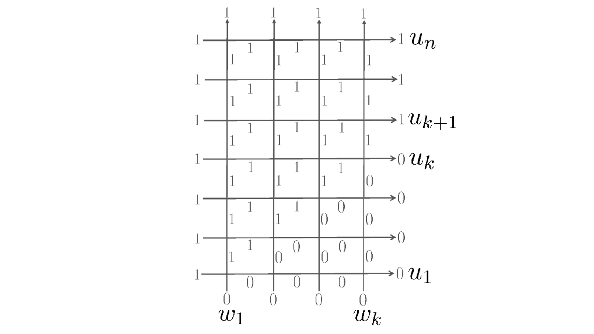
Refer to caption
Figure 6: The partition function ⟨0k1n−k|∏j∈SkmC¯(wj|u1,…,un)|Ω¯⟩nn\displaystyle{}_{n}\langle 0^{k}1^{n-k}|\prod_{j\in S_{k}^{m}}\overline{C}(w_{j}|u_{1},\dots,u_{n})|\overline{\Omega}\rangle_{n}. We note that only one configuration is allowed, from which one can see ⟨0k1n−k|∏j∈SkmC¯(wj|u1,…,un)|Ω¯⟩nn=∏j=1nujk\displaystyle{}_{n}\langle 0^{k}1^{n-k}|\prod_{j\in S_{k}^{m}}\overline{C}(w_{j}|u_{1},\dots,u_{n})|\overline{\Omega}\rangle_{n}=\prod_{j=1}^{n}u_{j}^{k}.
∏j=k+1mA¯​(wj|u1,…,un)​∏j=1kC¯​(wj|u1,…,un)\displaystyle\prod_{j=k+1}^{m}\overline{A}(w_{j}|u_{1},\dots,u_{n})\prod_{j=1}^{k}\overline{C}(w_{j}|u_{1},\dots,u_{n})
=\displaystyle= ∑Skm∈([m]k)∏i∈Skm,j∈Skm¯wiwi−wj​∏j∈SkmC¯​(wj|u1,…,un)​∏j∈Skm¯A¯​(wj|u1,…,un).\displaystyle\sum_{S_{k}^{m}\in\binom{[m]}{k}}\prod_{i\in S_{k}^{m},j\in\overline{S_{k}^{m}}}\frac{w_{i}}{w_{i}-w_{j}}\prod_{j\in S_{k}^{m}}\overline{C}(w_{j}|u_{1},\dots,u_{n})\prod_{j\in\overline{S_{k}^{m}}}\overline{A}(w_{j}|u_{1},\dots,u_{n}). (4.10)

Using (4.10) and the action of the AA-operators on the state |Ω¯⟩n|\overline{\Omega}\rangle_{n}

∏j∈Skm¯A¯​(wj|u1,…,un)​|Ω¯⟩n=∏j∈Skm¯∏i=1n(ui−wj)​|Ω¯⟩n,\displaystyle\prod_{j\in\overline{S_{k}^{m}}}\overline{A}(w_{j}|u_{1},\dots,u_{n})|\overline{\Omega}\rangle_{n}=\prod_{j\in\overline{S_{k}^{m}}}\prod_{i=1}^{n}(u_{i}-w_{j})|\overline{\Omega}\rangle_{n}, (4.11)

(4.4) can be rewritten as

Wm+n−k,n(u1,…,un|w1,…,wm+n−k|1,…,k,m+1,…,m+n−k)\displaystyle W_{m+n-k,n}(u_{1},\dots,u_{n}|w_{1},\dots,w_{m+n-k}|1,\dots,k,m+1,\dots,m+n-k)
=\displaystyle= ∏j=1nujn−k∑Skm∈([m]k)∏i∈Skm,j∈Skm¯wiwi−wj∏j∈Skm¯∏i=1n(ui−wj)⟨0k1n−k|∏j∈SkmC¯(wj|u1,…,un)|Ω¯⟩nn.\displaystyle\prod_{j=1}^{n}u_{j}^{n-k}\sum_{S_{k}^{m}\in\binom{[m]}{k}}\prod_{i\in S_{k}^{m},j\in\overline{S_{k}^{m}}}\frac{w_{i}}{w_{i}-w_{j}}\prod_{j\in\overline{S_{k}^{m}}}\prod_{i=1}^{n}(u_{i}-w_{j}){}_{n}\langle 0^{k}1^{n-k}|\prod_{j\in S_{k}^{m}}\overline{C}(w_{j}|u_{1},\dots,u_{n})|\overline{\Omega}\rangle_{n}. (4.12)

One can easily see from the graphical description that the partition function
⟨0k1n−k|∏j∈SkmC¯(wj|u1,…,un)|Ω¯⟩nn\displaystyle{}_{n}\langle 0^{k}1^{n-k}|\prod_{j\in S_{k}^{m}}\overline{C}(w_{j}|u_{1},\dots,u_{n})|\overline{\Omega}\rangle_{n} is completely frozen (Figure 6), and find that its explicit form is given by

⟨0k1n−k|∏j∈SkmC¯(wj|u1,…,un)|Ω¯⟩nn=∏j=1nujk.\displaystyle{}_{n}\langle 0^{k}1^{n-k}|\prod_{j\in S_{k}^{m}}\overline{C}(w_{j}|u_{1},\dots,u_{n})|\overline{\Omega}\rangle_{n}=\prod_{j=1}^{n}u_{j}^{k}. (4.13)

Substituting (4.13) into (4.12), we get

Wm+n−k,n(u1,…,un|w1,…,wm+n−k|1,…,k,m+1,…,m+n−k)\displaystyle W_{m+n-k,n}(u_{1},\dots,u_{n}|w_{1},\dots,w_{m+n-k}|1,\dots,k,m+1,\dots,m+n-k)
=\displaystyle= ∏j=1nujn​∑Skm∈([m]k)∏i∈Skm,j∈Skm¯wiwi−wj​∏j∈Skm¯∏i=1n(ui−wj).\displaystyle\prod_{j=1}^{n}u_{j}^{n}\sum_{S_{k}^{m}\in\binom{[m]}{k}}\prod_{i\in S_{k}^{m},j\in\overline{S_{k}^{m}}}\frac{w_{i}}{w_{i}-w_{j}}\prod_{j\in\overline{S_{k}^{m}}}\prod_{i=1}^{n}(u_{i}-w_{j}). (4.14)

Finally, we compare the two expressions (4.3) and (4.14) to get

∏j=1n1(1−zj)m+n−k​G((m−k)n−k,0k)​({z1,…,zn}|𝜶)\displaystyle\prod_{j=1}^{n}\frac{1}{(1-z_{j})^{m+n-k}}G_{((m-k)^{n-k},0^{k})}(\{z_{1},\dots,z_{n}\}|\boldsymbol{\alpha})
=\displaystyle= ∏j=1nujn​∑Skm∈([m]k)∏i∈Skm,j∈Skm¯wiwi−wj​∏j∈Skm¯∏i=1n(ui−wj),\displaystyle\prod_{j=1}^{n}u_{j}^{n}\sum_{S_{k}^{m}\in\binom{[m]}{k}}\prod_{i\in S_{k}^{m},j\in\overline{S_{k}^{m}}}\frac{w_{i}}{w_{i}-w_{j}}\prod_{j\in\overline{S_{k}^{m}}}\prod_{i=1}^{n}(u_{i}-w_{j}), (4.15)

which, after using the translation rule zj=1−uj−1​(j=1,…,n)z_{j}=1-u_{j}^{-1}\ (j=1,\dots,n), αj=1−wj​(j=1,…,m+n−k)\alpha_{j}=1-w_{j}\ (j=1,\dots,m+n-k), becomes the identity

G((m−k)n−k,0k)​(𝒛|𝜶)=∑Skm∈([m]k)∏i∈Skm(1−αi)m−k​∏j∈Skm¯∏i=1n(zi⊕αj)∏i∈Skm∏j∈Skm¯(αj−αi).\displaystyle G_{((m-k)^{n-k},0^{k})}(\boldsymbol{z}|\boldsymbol{\alpha})=\sum_{S_{k}^{m}\in\binom{[m]}{k}}\frac{\displaystyle\prod_{i\in{S_{k}^{m}}}(1-\alpha_{i})^{m-k}\prod_{j\in\overline{S_{k}^{m}}}\prod_{i=1}^{n}(z_{i}\oplus\alpha_{j})}{\displaystyle\prod_{i\in{S_{k}^{m}}}\prod_{j\in\overline{{S_{k}^{m}}}}(\alpha_{j}-\alpha_{i})}. (4.16)

∎

Example of Theorem 4.1
When n=2n=2, k=1k=1, m=2m=2, the right hand side of (4.1) is

(1−α1)​(z1⊕α2)​(z2⊕α2)α2−α1+(1−α2)​(z1⊕α1)​(z2⊕α1)α1−α2\displaystyle\frac{(1-\alpha_{1})(z_{1}\oplus\alpha_{2})(z_{2}\oplus\alpha_{2})}{\alpha_{2}-\alpha_{1}}+\frac{(1-\alpha_{2})(z_{1}\oplus\alpha_{1})(z_{2}\oplus\alpha_{1})}{\alpha_{1}-\alpha_{2}}
=\displaystyle= (α1​α2−α1−α2+1)​(z1+z2−z1​z2)+α1+α2−α1​α2,\displaystyle(\alpha_{1}\alpha_{2}-\alpha_{1}-\alpha_{2}+1)(z_{1}+z_{2}-z_{1}z_{2})+\alpha_{1}+\alpha_{2}-\alpha_{1}\alpha_{2}, (4.17)

which gives the left hand side G(1,0)​({z1,z2}|𝜶)G_{(1,0)}(\{z_{1},z_{2}\}|\boldsymbol{\alpha}).

Combining (4.1) with the Guo-Sun identity (1.3) for the case λ1=⋯=λk=0\lambda_{1}=\cdots=\lambda_{k}=0 and using G(0,…,0)​(𝒛Skn|𝜶)=1G_{(0,\dots,0)}(\boldsymbol{z}_{S_{k}^{n}}|\boldsymbol{\alpha})=1, we get the following duality formula.

Theorem 4.2.

The following identity holds:

∑Skn∈([n]k)∏i∈Skn(1−zi)n−k​∏j∈Skn¯∏i=1m(zj⊕αi)∏i∈Skn∏j∈Skn¯(zj−zi)\displaystyle\sum_{S_{k}^{n}\in\binom{[n]}{k}}\frac{\displaystyle\prod_{i\in{S_{k}^{n}}}(1-z_{i})^{n-k}\prod_{j\in\overline{S_{k}^{n}}}\prod_{i=1}^{m}(z_{j}\oplus\alpha_{i})}{\displaystyle\prod_{i\in{S_{k}^{n}}}\prod_{j\in\overline{{S_{k}^{n}}}}(z_{j}-z_{i})}
=\displaystyle= ∑Skm∈([m]k)∏i∈Skm(1−αi)m−k​∏j∈Skm¯∏i=1n(zi⊕αj)∏i∈Skm∏j∈Skm¯(αj−αi).\displaystyle\sum_{S_{k}^{m}\in\binom{[m]}{k}}\frac{\displaystyle\prod_{i\in{S_{k}^{m}}}(1-\alpha_{i})^{m-k}\prod_{j\in\overline{S_{k}^{m}}}\prod_{i=1}^{n}(z_{i}\oplus\alpha_{j})}{\displaystyle\prod_{i\in{S_{k}^{m}}}\prod_{j\in\overline{{S_{k}^{m}}}}(\alpha_{j}-\alpha_{i})}. (4.18)

5 A qq-deformation

In this section, we discuss a qq-deformation of the Guo-Sun identity. We follow the same procedure of computation in section 3 done for the five-vertex model. Now we consider the Uq​(s​l2^)U_{q}(\widehat{sl_{2}}) six-vertex model whose RR-matrix is given by (2). Recall that the correspondence between the wavefunctions of the six-vertex model and the symmetric functions (2.13) are given by (2.14), which applied to the one Wm+n−k,n(u1,…,un|w1,…,wm+n−k|x1,…,xk,m+1,…,m+n−k)W_{m+n-k,n}(u_{1},\dots,u_{n}|w_{1},\dots,w_{m+n-k}|x_{1},\dots,x_{k},m+1,\dots,m+n-k) we deal with in this section, becomes

Wm+n−k,n(u1,…,un|w1,…,wm+n−k|x1,…,xk,m+1,…,m+n−k)\displaystyle W_{m+n-k,n}(u_{1},\dots,u_{n}|w_{1},\dots,w_{m+n-k}|x_{1},\dots,x_{k},m+1,\dots,m+n-k)
=\displaystyle= Fm+n−k,n(u1,…,un|w1,…,wm+n−k|x1,…,xk,m+1,…,m+n−k).\displaystyle F_{m+n-k,n}(u_{1},\dots,u_{n}|w_{1},\dots,w_{m+n-k}|x_{1},\dots,x_{k},m+1,\dots,m+n-k). (5.1)
Refer to caption
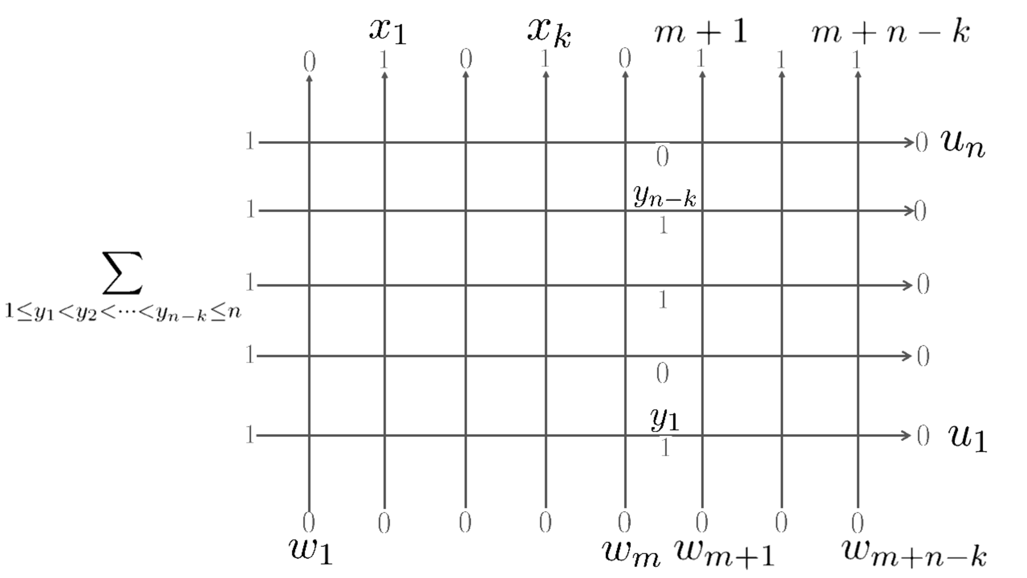
Figure 7: The decomposition of the wavefunctions (5.2). From the ice rule of the RR-matrix of the six-vertex model and the boundary condition, we note that for every allowed configuration, the states on the horizontal edges between the mm-th and the (m+1)(m+1)-th column consist of (n−k)(n-k) 1’s and kk 0’s. We label the positions of the (n−k)(n-k) 1’s as y1,y2,…,yn−ky_{1},y_{2},\dots,y_{n-k} (1≤y1<y2<⋯<yn−k≤n1\leq y_{1}<y_{2}<\cdots<y_{n-k}\leq n), starting from the bottom row.

Next we examine Wm+n−k,n(u1,…,un|w1,…,wm+n−k|x1,…,xk,m+1,…,m+n−k)W_{m+n-k,n}(u_{1},\dots,u_{n}|w_{1},\dots,w_{m+n-k}|x_{1},\dots,x_{k},m+1,\dots,m+n-k) from another point of view as in section 3. Unlike the case for the five-vertex model, there are several allowed configurations in the rightmost n−kn-k columns (for the five-vertex model, only one configuration is allowed). However, from the the so-called ice rule ⟨γ|⟨δ|Ra​b(u,w)|α⟩ab|β⟩ba=0{}_{a}\langle\gamma|{}_{b}\langle\delta|R_{ab}(u,w)|\alpha\rangle_{a}|\beta\rangle_{b}=0 unless α+β=γ+δ\alpha+\beta=\gamma+\delta and since the states at the right boundary are all ⟨0|\langle 0|, one can see that the wavefunctions can be decomposed as (Figure 7)

Wm+n−k,n(u1,…,un|w1,…,wm+n−k|x1,…,xk,m+1,…,m+n−k)\displaystyle W_{m+n-k,n}(u_{1},\dots,u_{n}|w_{1},\dots,w_{m+n-k}|x_{1},\dots,x_{k},m+1,\dots,m+n-k)
=\displaystyle= ∑1≤y1<y2<⋯<yn−k≤nW¯n,n−k(wm+1,…,wm+n−k|u1,…,un|y1,…,yn−k)\displaystyle\sum_{1\leq y_{1}<y_{2}<\cdots<y_{n-k}\leq n}\overline{W}_{n,n-k}(w_{m+1},\dots,w_{m+n-k}|u_{1},\dots,u_{n}|y_{1},\dots,y_{n-k})
×\displaystyle\times ⟨x1,…,xk|∏j=yn−k+1nB(uj|w1,…,wm)D(uyn−k|w1,…,wm)∏j=yn−k−1+1yn−k−1B(uj|w1,…,wm)m\displaystyle{}_{m}\langle x_{1},\dots,x_{k}|\prod_{j=y_{n-k}+1}^{n}B(u_{j}|w_{1},\dots,w_{m})D(u_{y_{n-k}}|w_{1},\dots,w_{m})\prod_{j=y_{n-k-1}+1}^{y_{n-k}-1}B(u_{j}|w_{1},\dots,w_{m})
×\displaystyle\times ⋯×∏j=y1+1y2−1B⁡(uj|w1,…,wm)​D​(uy1|w1,…,wm)​∏j=1y1−1B⁡(uj|w1,…,wm)​|Ω⟩m,\displaystyle\cdots\times\prod_{j=y_{1}+1}^{y_{2}-1}B(u_{j}|w_{1},\dots,w_{m})D(u_{y_{1}}|w_{1},\dots,w_{m})\prod_{j=1}^{y_{1}-1}B(u_{j}|w_{1},\dots,w_{m})|\Omega\rangle_{m}, (5.2)

where

W¯n,n−k(wm+1,…,wm+n−k|u1,…,un|y1,…,yn−k)\displaystyle\overline{W}_{n,n-k}(w_{m+1},\dots,w_{m+n-k}|u_{1},\dots,u_{n}|y_{1},\dots,y_{n-k})
=\displaystyle= ⟨1|⊗⋯⊗⟨1|∏j=yn−k+1nA(uj|wm+1,…,wm+n−k)B(uyn−k|wm+1,…,wm+n−k)m+n−km+1\displaystyle{}_{m+1}\langle 1|\otimes\cdots\otimes{}_{m+n-k}\langle 1|\prod_{j=y_{n-k}+1}^{n}A(u_{j}|w_{m+1},\dots,w_{m+n-k})B(u_{y_{n-k}}|w_{m+1},\dots,w_{m+n-k})
×\displaystyle\times ∏j=yn−k−1+1yn−k−1A(uj|wm+1,…,wm+n−k)⋯×∏j=y1+1y2−1A(uj|wm+1,…,wm+n−k)\displaystyle\prod_{j=y_{n-k-1}+1}^{y_{n-k}-1}A(u_{j}|w_{m+1},\dots,w_{m+n-k})\cdots\times\prod_{j=y_{1}+1}^{y_{2}-1}A(u_{j}|w_{m+1},\dots,w_{m+n-k})
×\displaystyle\times B(uy1|wm+1,…,wm+n−k)∏j=1y1−1A(uj|wm+1,…,wm+n−k)|0⟩m+n−k⊗⋯⊗|0⟩m+1.\displaystyle B(u_{y_{1}}|w_{m+1},\dots,w_{m+n-k})\prod_{j=1}^{y_{1}-1}A(u_{j}|w_{m+1},\dots,w_{m+n-k})|0\rangle_{m+n-k}\otimes\cdots\otimes|0\rangle_{m+1}. (5.3)

W¯n,n−k(wm+1,…,wm+n−k|u1,…,un|y1,…,yn−k)\overline{W}_{n,n-k}(w_{m+1},\dots,w_{m+n-k}|u_{1},\dots,u_{n}|y_{1},\dots,y_{n-k}) is another class of wavefunctions and one can show the following correspondence

W¯n,n−k(wm+1,…,wm+n−k|u1,…,un|y1,…,yn−k)\displaystyle\overline{W}_{n,n-k}(w_{m+1},\dots,w_{m+n-k}|u_{1},\dots,u_{n}|y_{1},\dots,y_{n-k})
=\displaystyle= F¯n,n−k(wm+1,…,wm+n−k|u1,…,un|y1,…,yn−k),\displaystyle\overline{F}_{n,n-k}(w_{m+1},\dots,w_{m+n-k}|u_{1},\dots,u_{n}|y_{1},\dots,y_{n-k}), (5.4)

where F¯n,n−k(wm+1,…,wm+n−k|u1,…,un|y1,…,yn−k)\overline{F}_{n,n-k}(w_{m+1},\dots,w_{m+n-k}|u_{1},\dots,u_{n}|y_{1},\dots,y_{n-k}) is the following symmetric functions with symmetric variables wm+1,…,wm+n−kw_{m+1},\dots,w_{m+n-k}, another set of variables u1,…,unu_{1},\dots,u_{n} and a set of integers y1,…,yn−ky_{1},\dots,y_{n-k} satisfying 1≤y1<y2<⋯<yn−k≤n1\leq y_{1}<y_{2}<\cdots<y_{n-k}\leq n

F¯n,n−k(wm+1,…,wm+n−k|u1,…,un|y1,…,yn−k)\displaystyle\overline{F}_{n,n-k}(w_{m+1},\dots,w_{m+n-k}|u_{1},\dots,u_{n}|y_{1},\dots,y_{n-k})
=\displaystyle= ∑σ∈Sn−k∏j=1n−k∏i=yj+1nq⁡(ui−wm+σ⁡(j))​∏1≤i<j≤n−kq​wm+σ⁡(i)−wm+σ⁡(j)q⁡(wm+σ⁡(i)−wm+σ⁡(j))\displaystyle\sum_{\sigma\in S_{n-k}}\prod_{j=1}^{n-k}\prod_{i=y_{j}+1}^{n}q(u_{i}-w_{m+\sigma(j)})\prod_{1\leq i<j\leq n-k}\frac{qw_{m+\sigma(i)}-w_{m+\sigma(j)}}{q(w_{m+\sigma(i)}-w_{m+\sigma(j)})}
×∏j=1n−k∏i=1yj−1(ui−q​wm+σ⁡(j))​∏j=1n−k(1−q)​uyj.\displaystyle\times\prod_{j=1}^{n-k}\prod_{i=1}^{y_{j}-1}(u_{i}-qw_{m+\sigma(j)})\prod_{j=1}^{n-k}(1-q)u_{y_{j}}. (5.5)

One can show the correspondence (5.4) for example by the Izergin-Korepin method [27, 28], which can be applied to the wavefunctions [24] as follows. First, we construct the following Korepin’s lemma which list the properties of the partition functions which uniquely characterize them. For the case of the wavefunctions W¯n,n−k(wm+1,…,wm+n−k|u1,…,un|y1,…,yn−k)\overline{W}_{n,n-k}(w_{m+1},\dots,w_{m+n-k}|u_{1},\dots,u_{n}|y_{1},\dots,y_{n-k}), the Korepin’s Lemma is given below.

Proposition 5.1.

The partition functions W¯n,n−k(wm+1,…,wm+n−k|u1,…,un|y1,…,yn−k)\overline{W}_{n,n-k}(w_{m+1},\dots,w_{m+n-k}|u_{1},\dots,u_{n}|y_{1},\dots,y_{n-k}) satisfies the following properties.

(1) W¯n,n−k(wm+1,…,wm+n−k|u1,…,un|y1,…,yn−k)\overline{W}_{n,n-k}(w_{m+1},\dots,w_{m+n-k}|u_{1},\dots,u_{n}|y_{1},\dots,y_{n-k}) is a polynomial of degree n−kn-k in unu_{n} if yn−k=ny_{n-k}=n.

(2) W¯n,n−k(wm+1,…,wm+n−k|u1,…,un|y1,…,yn−k)\overline{W}_{n,n-k}(w_{m+1},\dots,w_{m+n-k}|u_{1},\dots,u_{n}|y_{1},\dots,y_{n-k}) is symmetric with respect to wjw_{j}, j=m+1,…,m+n−kj=m+1,\dots,m+n-k.

(3) The following recursive relations between the partition functions hold if yn−k=ny_{n-k}=n:

W¯n,n−k(wm+1,…,wm+n−k|u1,…,un|y1,…,yn−k)|un=0=0,\displaystyle\overline{W}_{n,n-k}(w_{m+1},\dots,w_{m+n-k}|u_{1},\dots,u_{n}|y_{1},\dots,y_{n-k})|_{u_{n}=0}=0, (5.6)
W¯n,n−k(wm+1,…,wm+n−k|u1,…,un|y1,…,yn−k)|un=wm+n−k\displaystyle\overline{W}_{n,n-k}(w_{m+1},\dots,w_{m+n-k}|u_{1},\dots,u_{n}|y_{1},\dots,y_{n-k})|_{u_{n}=w_{m+n-k}}
=\displaystyle= (1−q)​wm+n−k​∏j=m+1m+n−k−1(wm+n−k−q​wj)​∏j=1n−1(uj−q​wm+n−k)\displaystyle(1-q)w_{m+n-k}\prod_{j=m+1}^{m+n-k-1}(w_{m+n-k}-qw_{j})\prod_{j=1}^{n-1}(u_{j}-qw_{m+n-k})
×W¯n−1,n−k−1(wm+1,…,wm+n−k−1|u1,…,un−1|y1,…,yn−k−1).\displaystyle\times\overline{W}_{n-1,n-k-1}(w_{m+1},\dots,w_{m+n-k-1}|u_{1},\dots,u_{n-1}|y_{1},\dots,y_{n-k-1}). (5.7)

If yn−k≠ny_{n-k}\neq n, the following factorizations hold for the wavefunctions:

W¯n,n−k(wm+1,…,wm+n−k|u1,…,un|y1,…,yn−k)\displaystyle\overline{W}_{n,n-k}(w_{m+1},\dots,w_{m+n-k}|u_{1},\dots,u_{n}|y_{1},\dots,y_{n-k})
=\displaystyle= ∏j=m+1m+n−kq(un−wj)W¯n−1,n−k(wm+1,…,wm+n−k|u1,…,un−1|y1,…,yn−k).\displaystyle\prod_{j=m+1}^{m+n-k}q(u_{n}-w_{j})\overline{W}_{n-1,n-k}(w_{m+1},\dots,w_{m+n-k}|u_{1},\dots,u_{n-1}|y_{1},\dots,y_{n-k}). (5.8)

(4) The following holds for the case n−k=1n-k=1, y1=ny_{1}=n

W¯n,1(wm+1|u1,…,un|n)=(1−q)un∏j=1n−1(uj−qwm+1).\displaystyle\overline{W}_{n,1}(w_{m+1}|u_{1},\dots,u_{n}|n)=(1-q)u_{n}\prod_{j=1}^{n-1}(u_{j}-qw_{m+1}). (5.9)

After constructing Korepin’s Lemma, by showing that the symmetric functions
F¯n,n−k(wm+1,…,wm+n−k|u1,…,un|y1,…,yn−k)\overline{F}_{n,n-k}(w_{m+1},\dots,w_{m+n-k}|u_{1},\dots,u_{n}|y_{1},\dots,y_{n-k}) satisfy all the properties in Proposition 5.1 and we get the correspondence (5.4).

Now we examine the factors

⟨x1,…,xk|∏j=yn−k+1nB(uj|w1,…,wm)D(uyn−k|w1,…,wm)∏j=yn−k−1+1yn−k−1B(uj|w1,…,wm)m\displaystyle{}_{m}\langle x_{1},\dots,x_{k}|\prod_{j=y_{n-k}+1}^{n}B(u_{j}|w_{1},\dots,w_{m})D(u_{y_{n-k}}|w_{1},\dots,w_{m})\prod_{j=y_{n-k-1}+1}^{y_{n-k}-1}B(u_{j}|w_{1},\dots,w_{m})
×\displaystyle\times ⋯×∏j=y1+1y2−1B⁡(uj|w1,…,wm)​D​(uy1|w1,…,wm)​∏j=1y1−1B⁡(uj|w1,…,wm)​|Ω⟩m,\displaystyle\cdots\times\prod_{j=y_{1}+1}^{y_{2}-1}B(u_{j}|w_{1},\dots,w_{m})D(u_{y_{1}}|w_{1},\dots,w_{m})\prod_{j=1}^{y_{1}-1}B(u_{j}|w_{1},\dots,w_{m})|\Omega\rangle_{m}, (5.10)

in (5.2). We apply the method used in [29] to study correlation functions of the XXZ spin chain for simplifying (5.10). From the intertwining relation (3.3) for the six-vertex model (2), we get

D⁡(u1)​B​(u2)\displaystyle D(u_{1})B(u_{2}) =u1−q​u2u1−u2​B​(u2)​D​(u1)+(q−1)​u2u1−u2​B​(u1)​D​(u2),\displaystyle=\frac{u_{1}-qu_{2}}{u_{1}-u_{2}}B(u_{2})D(u_{1})+\frac{(q-1)u_{2}}{u_{1}-u_{2}}B(u_{1})D(u_{2}), (5.11)
B⁡(u1)​B​(u2)\displaystyle B(u_{1})B(u_{2}) =B⁡(u2)​B​(u1).\displaystyle=B(u_{2})B(u_{1}). (5.12)

From the argument which is standard in the algebraic Bethe ansatz, we can combine (5.11), (5.12) and

D⁡(u|w1,…,wm)​|Ω⟩m=∏i=1m(u−wi)​|Ω⟩m,\displaystyle D(u|w_{1},\dots,w_{m})|\Omega\rangle_{m}=\prod_{i=1}^{m}(u-w_{i})|\Omega\rangle_{m}, (5.13)

to show the following relation

D⁡(uℓ+1|w1,…,wm)​∏j=1ℓB⁡(uj|w1,…,wm)​|Ω⟩m\displaystyle D(u_{\ell+1}|w_{1},\dots,w_{m})\prod_{j=1}^{\ell}B(u_{j}|w_{1},\dots,w_{m})|\Omega\rangle_{m}
=\displaystyle= ∑k=1ℓ+1∏i=1m(uk−wi)​∏j=1ℓ(uk−q​uj)∏j=1j≠kℓ+1(uk−uj)​∏j=1j≠kℓ+1B⁡(uj|w1,…,wm)​|Ω⟩m.\displaystyle\sum_{k=1}^{\ell+1}\prod_{i=1}^{m}(u_{k}-w_{i})\frac{\displaystyle\prod_{j=1}^{\ell}(u_{k}-qu_{j})}{\displaystyle\prod_{\begin{subarray}{c}j=1\\ j\neq k\end{subarray}}^{\ell+1}(u_{k}-u_{j})}\prod_{\begin{subarray}{c}j=1\\ j\neq k\end{subarray}}^{\ell+1}B(u_{j}|w_{1},\dots,w_{m})|\Omega\rangle_{m}. (5.14)

Using (5.14) repeatedly, one gets

∏j=yn−k+1nB⁡(uj|w1,…,wm)​D​(uyn−k|w1,…,wm)​∏j=yn−k−1+1yn−k−1B⁡(uj|w1,…,wm)\displaystyle\prod_{j=y_{n-k}+1}^{n}B(u_{j}|w_{1},\dots,w_{m})D(u_{y_{n-k}}|w_{1},\dots,w_{m})\prod_{j=y_{n-k-1}+1}^{y_{n-k}-1}B(u_{j}|w_{1},\dots,w_{m})
×\displaystyle\times ⋯×∏j=y1+1y2−1B⁡(uj|w1,…,wm)​D​(uy1|w1,…,wm)​∏j=1y1−1B⁡(uj|w1,…,wm)​|Ω⟩m\displaystyle\cdots\times\prod_{j=y_{1}+1}^{y_{2}-1}B(u_{j}|w_{1},\dots,w_{m})D(u_{y_{1}}|w_{1},\dots,w_{m})\prod_{j=1}^{y_{1}-1}B(u_{j}|w_{1},\dots,w_{m})|\Omega\rangle_{m}
=\displaystyle= ∑a1=1y1∑a2=1a2≠a1y2⋯∑an−k=1an−k≠a1,…,an−k−1yn−k∏j=1n−k∏i=1m(uaj−wi)∏j=1n−k∏b=1b≠a1,…,aj−1yj−1(uaj−q​ub)∏j=1n−k∏b=1b≠a1,…,ajyj(uaj−ub)\displaystyle\sum_{a_{1}=1}^{y_{1}}\sum_{\begin{subarray}{c}a_{2}=1\\ a_{2}\neq a_{1}\end{subarray}}^{y_{2}}\cdots\sum_{\begin{subarray}{c}a_{n-k}=1\\ a_{n-k}\neq a_{1},\dots,a_{n-k-1}\end{subarray}}^{y_{n-k}}\prod_{j=1}^{n-k}\prod_{i=1}^{m}(u_{a_{j}}-w_{i})\frac{\displaystyle\prod_{j=1}^{n-k}\prod_{\begin{subarray}{c}b=1\\ b\neq a_{1},\dots,a_{j-1}\end{subarray}}^{y_{j}-1}(u_{a_{j}}-qu_{b})}{\displaystyle\prod_{j=1}^{n-k}\prod_{\begin{subarray}{c}b=1\\ b\neq a_{1},\dots,a_{j}\end{subarray}}^{y_{j}}(u_{a_{j}}-u_{b})}
×\displaystyle\times ∏j=1j≠a1,…,an−knB⁡(uj|w1,…,wm)​|Ω⟩m.\displaystyle\prod_{\begin{subarray}{c}j=1\\ j\neq a_{1},\dots,a_{n-k}\end{subarray}}^{n}B(u_{j}|w_{1},\dots,w_{m})|\Omega\rangle_{m}. (5.15)

Combining (5.15) and the correspondence

⟨x1,…,xk|∏j=1j≠a1,…,an−knB(uj|w1,…,wm)|Ω⟩mm\displaystyle{}_{m}\langle x_{1},\dots,x_{k}|\prod_{\begin{subarray}{c}j=1\\ j\neq a_{1},\dots,a_{n-k}\end{subarray}}^{n}B(u_{j}|w_{1},\dots,w_{m})|\Omega\rangle_{m}
=\displaystyle= Wm,n({u1,…,un}\{ua1,…,uan−k}|w1,…,wm|x1,…,xk),\displaystyle W_{m,n}(\{u_{1},\dots,u_{n}\}\backslash\{u_{a_{1}},\dots,u_{a_{n-k}}\}|w_{1},\dots,w_{m}|x_{1},\dots,x_{k}), (5.16)

(5.10) becomes

⟨x1,…,xk|∏j=yn−k+1nB(uj|w1,…,wm)D(uyn−k|w1,…,wm)∏j=yn−k−1+1yn−k−1B(uj|w1,…,wm)m\displaystyle{}_{m}\langle x_{1},\dots,x_{k}|\prod_{j=y_{n-k}+1}^{n}B(u_{j}|w_{1},\dots,w_{m})D(u_{y_{n-k}}|w_{1},\dots,w_{m})\prod_{j=y_{n-k-1}+1}^{y_{n-k}-1}B(u_{j}|w_{1},\dots,w_{m})
×\displaystyle\times ⋯×∏j=y1+1y2−1B⁡(uj|w1,…,wm)​D​(uy1|w1,…,wm)​∏j=1y1−1B⁡(uj|w1,…,wm)​|Ω⟩m\displaystyle\cdots\times\prod_{j=y_{1}+1}^{y_{2}-1}B(u_{j}|w_{1},\dots,w_{m})D(u_{y_{1}}|w_{1},\dots,w_{m})\prod_{j=1}^{y_{1}-1}B(u_{j}|w_{1},\dots,w_{m})|\Omega\rangle_{m}
=\displaystyle= ∑a1=1y1∑a2=1a2≠a1y2⋯∑an−k=1an−k≠a1,…,an−k−1yn−k∏j=1n−k∏i=1m(uaj−wi)∏j=1n−k∏b=1b≠a1,…,aj−1yj−1(uaj−q​ub)∏j=1n−k∏b=1b≠a1,…,ajyj(uaj−ub)\displaystyle\sum_{a_{1}=1}^{y_{1}}\sum_{\begin{subarray}{c}a_{2}=1\\ a_{2}\neq a_{1}\end{subarray}}^{y_{2}}\cdots\sum_{\begin{subarray}{c}a_{n-k}=1\\ a_{n-k}\neq a_{1},\dots,a_{n-k-1}\end{subarray}}^{y_{n-k}}\prod_{j=1}^{n-k}\prod_{i=1}^{m}(u_{a_{j}}-w_{i})\frac{\displaystyle\prod_{j=1}^{n-k}\prod_{\begin{subarray}{c}b=1\\ b\neq a_{1},\dots,a_{j-1}\end{subarray}}^{y_{j}-1}(u_{a_{j}}-qu_{b})}{\displaystyle\prod_{j=1}^{n-k}\prod_{\begin{subarray}{c}b=1\\ b\neq a_{1},\dots,a_{j}\end{subarray}}^{y_{j}}(u_{a_{j}}-u_{b})}
×\displaystyle\times Wm,n({u1,…,un}\{ua1,…,uan−k}|w1,…,wm|x1,…,xk).\displaystyle W_{m,n}(\{u_{1},\dots,u_{n}\}\backslash\{u_{a_{1}},\dots,u_{a_{n-k}}\}|w_{1},\dots,w_{m}|x_{1},\dots,x_{k}). (5.17)

Inserting (5.17) into the right hand side of (5.2), one gets

Wm+n−k,n(u1,…,un|w1,…,wm+n−k|x1,…,xk,m+1,…,m+n−k)\displaystyle W_{m+n-k,n}(u_{1},\dots,u_{n}|w_{1},\dots,w_{m+n-k}|x_{1},\dots,x_{k},m+1,\dots,m+n-k)
=\displaystyle= ∑1≤y1<y2<⋯<yn−k≤n∑a1=1y1∑a2=1a2≠a1y2⋯∑an−k=1an−k≠a1,…,an−k−1yn−k∏j=1n−k∏i=1m(uaj−wi)∏j=1n−k∏b=1b≠a1,…,aj−1yj−1(uaj−q​ub)∏j=1n−k∏b=1b≠a1,…,ajyj(uaj−ub)\displaystyle\sum_{1\leq y_{1}<y_{2}<\cdots<y_{n-k}\leq n}\sum_{a_{1}=1}^{y_{1}}\sum_{\begin{subarray}{c}a_{2}=1\\ a_{2}\neq a_{1}\end{subarray}}^{y_{2}}\cdots\sum_{\begin{subarray}{c}a_{n-k}=1\\ a_{n-k}\neq a_{1},\dots,a_{n-k-1}\end{subarray}}^{y_{n-k}}\prod_{j=1}^{n-k}\prod_{i=1}^{m}(u_{a_{j}}-w_{i})\frac{\displaystyle\prod_{j=1}^{n-k}\prod_{\begin{subarray}{c}b=1\\ b\neq a_{1},\dots,a_{j-1}\end{subarray}}^{y_{j}-1}(u_{a_{j}}-qu_{b})}{\displaystyle\prod_{j=1}^{n-k}\prod_{\begin{subarray}{c}b=1\\ b\neq a_{1},\dots,a_{j}\end{subarray}}^{y_{j}}(u_{a_{j}}-u_{b})}
×\displaystyle\times W¯n,n−k(wm+1,…,wm+n−k|u1,…,un|y1,…,yn−k)\displaystyle\overline{W}_{n,n-k}(w_{m+1},\dots,w_{m+n-k}|u_{1},\dots,u_{n}|y_{1},\dots,y_{n-k})
×\displaystyle\times Wm,n({u1,…,un}\{ua1,…,uan−k}|w1,…,wm|x1,…,xk),\displaystyle W_{m,n}(\{u_{1},\dots,u_{n}\}\backslash\{u_{a_{1}},\dots,u_{a_{n-k}}\}|w_{1},\dots,w_{m}|x_{1},\dots,x_{k}), (5.18)

which, using the correspondences (2.14) and (5.4), becomes an identity

Fm+n−k,n(u1,…,un|w1,…,wm+n−k|x1,…,xk,m+1,…,m+n−k)\displaystyle F_{m+n-k,n}(u_{1},\dots,u_{n}|w_{1},\dots,w_{m+n-k}|x_{1},\dots,x_{k},m+1,\dots,m+n-k)
=\displaystyle= ∑1≤y1<y2<⋯<yn−k≤n∑a1=1y1∑a2=1a2≠a1y2⋯∑an−k=1an−k≠a1,…,an−k−1yn−k∏j=1n−k∏i=1m(uaj−wi)∏j=1n−k∏b=1b≠a1,…,aj−1yj−1(uaj−q​ub)∏j=1n−k∏b=1b≠a1,…,ajyj(uaj−ub)\displaystyle\sum_{1\leq y_{1}<y_{2}<\cdots<y_{n-k}\leq n}\sum_{a_{1}=1}^{y_{1}}\sum_{\begin{subarray}{c}a_{2}=1\\ a_{2}\neq a_{1}\end{subarray}}^{y_{2}}\cdots\sum_{\begin{subarray}{c}a_{n-k}=1\\ a_{n-k}\neq a_{1},\dots,a_{n-k-1}\end{subarray}}^{y_{n-k}}\prod_{j=1}^{n-k}\prod_{i=1}^{m}(u_{a_{j}}-w_{i})\frac{\displaystyle\prod_{j=1}^{n-k}\prod_{\begin{subarray}{c}b=1\\ b\neq a_{1},\dots,a_{j-1}\end{subarray}}^{y_{j}-1}(u_{a_{j}}-qu_{b})}{\displaystyle\prod_{j=1}^{n-k}\prod_{\begin{subarray}{c}b=1\\ b\neq a_{1},\dots,a_{j}\end{subarray}}^{y_{j}}(u_{a_{j}}-u_{b})}
×\displaystyle\times F¯n,n−k(wm+1,…,wm+n−k|u1,…,un|y1,…,yn−k)\displaystyle\overline{F}_{n,n-k}(w_{m+1},\dots,w_{m+n-k}|u_{1},\dots,u_{n}|y_{1},\dots,y_{n-k})
×\displaystyle\times Fm,n({u1,…,un}\{ua1,…,uan−k}|w1,…,wm|x1,…,xk),\displaystyle F_{m,n}(\{u_{1},\dots,u_{n}\}\backslash\{u_{a_{1}},\dots,u_{a_{n-k}}\}|w_{1},\dots,w_{m}|x_{1},\dots,x_{k}), (5.19)

for the symmetric functions (2.13) and (5.5).

6 Conclusion

In this paper, from the point of view of quantum integrability, we first investigated the identity for the factorial Grothendieck polynomials found by Guo and Sun [1] which generalizes the one for the Schur polynomials by Fehér, Némethi and Rimányi [8]. We gave another proof by using the quantum inverse scattering method, which is a method to analyze quantum integrable models. Why the method can be used is based on the fact between the correspondence between the wavefunctions of a five-vertex model and the factorial Grothendieck polynomials. See [9, 10, 12, 13] also for previous works on the investigations of Cauchy-type identities, Gromov-Witten invariants and the Littlewood-Richardson coefficients using this correspondence.

We next used the same idea and technique “in another direction” to derive an identity for the factorial Grothendieck poylnomials of rectangular shapes. Combining the identity with the Guo-Sun identity, we obtained a duality formula. We also discussed a qq-deformation of the Guo-Sun identity, based on the correspondence between the wavefunctions of the Uq​(s​l2^)U_{q}(\widehat{sl_{2}}) six-vertex model and the qq-deformation of the factorial Grothendieck polynomials and following the same line of computation to prove the Guo-Sun identity. The identity obtained for the qq-deformed symmetric functions is rather much more complicated than the Guo-Sun identity since the six-vertex model is a more general model than the five-vertex model, and it is an interesting problem whether one can simplify the identity to a more compact form.

It may also be interesting to reexamine existing formulas for the Schur and Grothendieck polynomials from the viewpoint of quantum integrability, and apply the same idea and technique in different ways, cases and places to obtain new identities. It is also interesting to investigate if the integrability technique can be applied beyond Grassmannian Grothendieck polynomials. One needs first to investigate if the set-valued tableaux descriptions of more general Grothendieck polynomials in [30, 31, 32] can be translated into the language of integrable models.

Acknowledgments

The author thanks the referee for careful reading the manuscript and useful comments and suggestions. This work was partially supported by grant-in-Aid for and Scientific Research (C) No. 18K03205 and No. 16K05468.

References

  • [1] P.L. Guo, S.C.C. Sun, Identities on factorial Grothendieck polynomials, Adv. App. Math. 111 (2019) 101933.
  • [2] A. Lascoux, M. Schützenberger, Structure de Hopf de l’anneau de cohomologie et de l’anneau de Grothendieck d’une variété de drapeaux, C. R. Acad. Sci. Parix Sér. I Math 295 (1982) 629.
  • [3] S. Fomin, A.N. Kirillov, Grothendieck polynomials and the Yang-Baxter equation, Proc. 6th Internat. Conf. on Formal Power Series and Algebraic Combinatorics, DIMACS (1994) 183-190.
  • [4] A.S. Buch, A Littlewood-Richardson rule for the KK-theory of Grassmannians, Acta. Math. 189 (2002) 37.
  • [5] P.J. McNamara, Factorial Grothendieck Polynomials, Electron. J. Combin. 13 (2006) 71.
  • [6] T. Ikeda, H. Naruse, KK-theoretic analogues of factorial Schur PP-and QQ-functions, Adv. in Math. 243 (2013) 22.
  • [7] T. Ikeda, T. Shimazaki, A proof of KK-theoretic Littlewood-Richardson rules by Bender-Knuth-type involutions, Math. Res. Lett. 21 (2014) 333.
  • [8] L.M. Fehér, A. Némethi, R. Rimányi Equivariant classes of matrix matroid varieties, Comment. Math. Helv. 87 (2012) 861-889.
  • [9] K. Motegi and K. Sakai, Vertex models, TASEP and Grothendieck polynomials, J. Phys. A: Math. Theor. 46 (2013) 355201.
  • [10] K. Motegi, K. and Sakai, KK-theoretic boson-fermion correspondence and melting crystals, J. Phys. A: Math. Theor. 47 (2014) 445202.
  • [11] A.N. Kirillov, Notes on Schubert, Grothendieck and Key Polynomials, SIGMA 12 (2016) 034.
  • [12] V. Gorbounov, C. Korff, Quantum integrability and generalised quantum Schubert calculus, Adv. Math. 313 (2017) 282.
  • [13] M. Wheeler and P. Zinn-Justin, Littlewood-Richardson coefficients for Grothendieck polynomials from integrability, J. Reine Angew. Math. 757 (2019) 159.
  • [14] S. Iwao, H. Nagai, The discrete Toda equation revisited: dual β\beta-Grothendieck polynomials, ultradiscretization, and static solitons, J. Phys. A: Math. Theor. 51 (2018) 134002.
  • [15] S. Iwao, Grothendieck polynomials and the Boson-Fermion correspondence, e-print arXiv:1905.07692.
  • [16] C. Monical, O. Pechenik, T. Scrimshaw, Crystal structures for symmetric Grothendieck polynomials, e-print arXiv:1807.03294.
  • [17] V. Buciumas, T. Scrimshaw, K. Weber, Colored five-vertex models and Lascoux polynomials and atoms, e-print arXiv:1908.07364.
  • [18] L. D. Faddeev, E. K. Sklyanin, L. A. Takhtajan, The Quantum Inverse Problem Method. 1, Theor. Math. Phys. 40 (1979) 194.
  • [19] V. E. Korepin, N. M. Bogoliubov, A. G. Izergin, Quantum Inverse Scattering Method and Correlation Functions (Cambridge University Press, Cambridge, 1993).
  • [20] V. Drinfeld, Hopf algebras and the quantum Yang-Baxter equation, Sov. Math. Dokl. 32 (1985) 254.
  • [21] M. Jimbo, A qq-difference analogue of U⁡(g)U(g) and the Yang-Baxter equation, Lett. Math. Phys. 10 (1985) 63.
  • [22] E. H. Lieb, F.Y.Wu, Two-dimensional ferroelectric models, in Phase Transitions and Critical Phenomena (Academic Press, London, 1972), Vol. 1, pp. 331-490.
  • [23] A. Borodin, L. Petrov, Higher spin six vertex model and symmetric rational functions, Sel. Math. New Ser. 24 (2016) 751-874.
  • [24] K. Motegi, Symmetric functions and wavefunctions of XXZ-type six-vertex models and elliptic Felderhof models by Izergin-Korepin analysis, J. Math. Phys. 59 (2018) 053505.
  • [25] K. Shigechi, M. Uchiyama, Boxed skew plane partition and integrable phase model, J. Phys. A: Math. Gen. 38 (2005) 10287.
  • [26] N. M. Bogoliubov, Boxed plane partitions as an exactly solvable boson model, J. Phys. A 38 (2005) 9415.
  • [27] V. E. Korepin, Calculation of norms of Bethe wave functions, Commun. Math. Phys. 86 (1982) 391.
  • [28] A. Izergin, Partition function of the six-vertex model in a finite volume, Sov. Phys. Dokl. 32 (1987) 878.
  • [29] N. Kitanine, J.M. Maillet, V. Terras, Correlation functions of the XXZ Heisenberg spin-1/2 chain in a magnetic field, Nucl. Phys. B 567 (2000) 554-582.
  • [30] T. Matsumura, Flagged Grothendieck polynomials, J. Alg. Comb. 49 (2019) 209-228.
  • [31] T. Matsumura, S. Sugimoto, Factorial Flagged Grothendieck Polynomials, e-print arXiv:1903.02169.
  • [32] N.J.Y. Fan, P.L. Guo, Set-valued Rothe Tableaux and Grothendieck Polynomials, e-print arXiv:1908.04164.