Engineered thermalization and cooling of quantum many-body systems
Abstract
We develop a scheme for engineering genuine thermal states in analog quantum simulation platforms by coupling local degrees of freedom to driven, dissipative ancilla pseudospins. We demonstrate the scheme in a many-body quantum spin lattice simulation setting. A Born-Markov master equation describing the dynamics of the many-body system is developed, and we show that if the ancilla energies are periodically modulated, with a carefully chosen hierarchy of timescales, one can effectively thermalize the many-body system. Through analysis of the time-dependent dynamical generator, we determine the conditions under which the true thermal state is an approximate dynamical fixed point for general system Hamiltonians. Finally, we evaluate the thermalization protocol through numerical simulation and discuss prospects for implementation on current quantum simulation hardware.
I Introduction
Preparation of mixed states of many-body systems, particularly thermal states at low temperatures, is valuable for many scientific and algorithmic tasks, e.g., calculating finite temperature response of materials, Gibbs sampling for machine learning and optimization Brandao and Svore 2016; Kliesch et al. 2011; Riera et al. 2012. However, computing, or sampling from, such low temperature thermal states of large quantum (or classical) many-body systems is a notoriously difficult problem with a long history Binder and Heermann 2010; Landau and Binder 2014; Pang 2016. Analog quantum simulators, controllable experimental platforms that can be engineered to mimic and simulate quantum many-body systems Georgescu et al. 2014, present a new approach for preparing and sampling from complex states of such systems, including low-temperature thermal states. Despite this, most analog quantum simulation platforms typically focus on preparing pure quantum states of many-body systems . This is partly because preparing mixed states on many leading analog quantum simulation platforms, e.g., trapped cold atoms, is challenging due to the lack of scattering mechanisms needed to dissipate energy and thermalize Gross and Bloch 2017; Metcalf et al. 2016. Therefore, the thermalizing environment must be also engineered and simulated, which is challenging since such environments typically contain an immense number of degrees of freedom.
We develop a technique to engineer thermalization of many-body spin Hamiltonians based on coupling to driven, dissipative ancilla degrees of freedom (DOF) that effectively act as a tunable macroscopic bath. We derive a Born-Markov master equation describing the dynamics of a many-body system coupled to fast-relaxing, driven ancilla qubits, and show that if the ancilla energies are periodically modulated and swept across the system energy spectrum, with a carefully chosen hierarchy of timescales, one can effectively thermalize a many-body system. Combing the spectrum with ancillary spins has been proposed for ground-state cooling on digital quantum simulation platforms Kaplan et al. 2017; Polla et al. 2019, we extend these ideas by coupling ancilla driven to thermal equilibrium. We use analytic arguments and numerical investigations to demonstrate that the true thermal state is an approximate fixed point of the dynamics. The scheme we develop can be viewed as a protocol for filtering and transforming the structureless electromagnetic vacuum reservoir to a structured reservoir suitable for thermalizing the many-body quantum system at hand. This enables thermalization using a finite number of controlled ancilla DOF.
Our development of this thermalization protocol builds upon previous work that examined techniques for thermalizing systems governed by stabilizer Hamiltonians Herdman et al. 2010; Young et al. 2012. In these works, it was shown that many-body systems governed by a stabilizer Hamiltonians can be driven to their thermal states by weakly coupling driven and dissipated ancilla DOF. When one attempts to generalize the constructions in these works to achieve the goal of thermalizing an arbitrary many-body system, several issues arise. Stabilizer Hamiltonians possess local excitations, and therefore local couplings to ancilla DOF suffice to provide energy excitation and dampening. These Hamiltonians are harmonic in the sense that eigenstates within an excitation sector are separated by a constant (and known) energy – e.g., for the toric code, each quasiparticle excitation adds a known constant energy, depending only on whether it is a electric charge or magnetic vortex Kitaev and Laumann 2009. This implies that the ancilla DOFs that induce excitations can be tuned to a single energy (or few energies) to induce energy-conserving transitions between system and ancilla. Consequently, if Boltzmann populations are maintained in the ancilla DOFs, one can guarantee transition dynamics within the system that obey detailed balance. These observations are at the core of the stabilizer Hamiltonian thermalization protocol constructed in Young et al. 2012.
Systems governed by general Hamiltonians possess non-local excitations and non-uniform spectra. Therefore, one does not expect the stabilizer thermalization protocol to translate to a more general setting. However, we will show that by introducing a time-dependent, driven set of ancilla DOF one can formulate a slightly modified protocol that thermalizes systems governed by non-stabilizer Hamiltonians.
Our work is also motivated by the recent work by Shabani and Neven Shabani and Neven 2016 that studied how to engineer a reservoir to achieve thermalization of a quantum many-body system. gTheir constructions were based on approximating Kubo-Martin-Schwinger (KMS) conditions for equilibration, which the authors show can be achieved by suitably driving a large number of independent harmonic oscillators that together form an engineered reservoir. In this work we set out to demonstrate that thermalization is also possible with a reservoir composed of a small number of ancilla qudits (finite dimensional systems) when coupled with time-dependent driving and local dissipation. This significantly increases the practicality of the engineered thermalization scheme. It is important to point out that we do not make any guarantees on the thermalization time of our protocol. We expect that this will diverge with system size and inverse temperature for systems governed by Hamiltonians with hard to prepare ground states, such as QMA-hard Hamiltonians Kempe et al. 2006; Aharonov et al. 2009.
Finally, we note that there exist alternative thermalization protocols that exploit the Eigenstate Thermalization Hypothesis (ETH) and sample a subsystem of a larger system Anschuetz and Cao 2019. The state of this subsystem could be described by a thermal state if the ETH holds. These protocols do not possess a fully-controllable macroscopic bath and temperature must be determined by post-selection, therefore, it would be unlikely these methods can generate specific thermal states efficiently. In contrast our protocol does not require post-selection since the state of the many-body system converges to the thermal state.
The remainder of this paper is structured as follows. Section II presents the general model, thermalization protocol and discusses the relevant parameters. Section III derives a reduced equation of motion by averaging over the dynamics of the ancilla DOF in a carefully considered parameter regime. Then in section IV we discuss the importance of the detailed balance condition in dictating the accuracy of our thermalization protocol, and present analytic arguments for the properties of the steady state of our engineered evolution. section V presents several numerical simulation results that serve to illustrate our protocol and highlight some of its key properties, including its lack of accuracy in some regimes. Then we conclude in section VI with a brief discussion.
II The model
Consider a many-body Hamiltonian, describing coupled quantum spins. We will refer to the spin DOF governed by this Hamiltonian as the principal spins, and these are often localized to a regular lattice, see Fig. 1. We denote the eigenvalues and eigenvectors of by and , respectively.
Some subset of these principal spins are coupled to independent ancillary DOF that can also be described as quantum two-level systems, which we will refer to as ancilla spins. The coherent dynamics of the state of the combined system, living in the Hilbert space , is given by the time-dependent Hamiltonian ()
| (1) |
where () define Pauli spin operators on ancilla spin , and define Pauli operations on the principal spin. The ancilla spin energies are time-dependent, and we assume this dependence is periodic and takes the form where is the difference between the system Hamiltonian’s largest and smallest energy, and is a periodic function. The ancilla are coupled weakly to the system by an excitation exchange interaction between system spin and ancilla with coupling strength . Weak coupling of the system and bath is required for thermalization in the original eigenbasis of . In addition to this Hamiltonian, the ancilla spins must be driven to thermal equilibrium on a faster time-scale than the system-ancilla coupling timescale. We assume that each ancilla spin is driven (damped) at a rate () such that it effectively evolves according to the standard Markovian master equation:
| (2) | ||||
| (3) |
where is the density matrix for ancilla spin and with the Pauli raising (lowering) operator (). In the following, we will choose
| (4) |
with being the inverse temperature that we wish to thermalize the principal spin system to. Further, we choose the pumping parameter . In this regime the quasi-static fixed point of the ancilla spin’s evolution (which it reaches in roughly time) is a density matrix with Boltzmann distributed populations with respect to the inverse temperature and energy . One can engineer such an open-system evolution of a two-level system by encoding the two levels within a driven and dissipated (e.g., optically pumped) -atom (Steck 2013, Chap. 7.9), see Fig. 1. Importantly, direct dissipation of the principal spins does not lead to generation of a thermal state of the many-body system since the steady state in this case is dominated by locally thermalized spins (in a product state).
The number of ancilla () required and the choice of system-ancilla coupling (i.e., the value of and in each coupling ) is set by the requirement of ergodicity of dynamics of the system. Intuitively, this requirement states that it should be possible to transition from any eigenstate of to any other eigenstate through application of a sequence of ancilla-induced operations. We will state a concrete algebraic condition for ergodicity in the following section that can easily be checked. In practice, we have found that ergodicity is satisfied with at most ancilla spins (as long as the system-ancilla interactions do not commute with the system Hamiltonian).
Our thermalization protocol, which aims to drive the collective state of the principal spins to the Gibbs state under at inverse temperature , i.e., , proceeds by engineering the above interactions between the principal spins and ancilla spins and then sweeping all over a small number of periods. The intuition for why this should thermalize the principal system comes from noticing that at specified times, some set of ancilla spins is resonant with some energy gaps in , and since the ancilla spin populations are Boltzmann distributed, the interaction will drive populations in the resonant energy levels towards being Boltzmann distributed. Note that in this work we use the term “gap” to refer to any transition energy in the system, not just an energy difference between neighboring states. Over time and several cycles of the periodic modulation, as the ancilla spins become resonant with more and more energy gaps in all system populations will be driven to their thermal equilibrium populations. This intuitive description is what we formalize in the following sections.
III Reduced description of dynamics
Understanding the steady-state properties of the time-dependent evolution prescribed in the previous section is not possible without some simplifications. In order to gain insight into the evolution of the system under the protocol we find a particular parameter regime in which we can average over the ancilla spins and derive a time-dependent Markovian master equation governing the evolution of the principal spins alone.
In order to thermalize the system we need to be in a regime where the system “sees” each ancilla energy for some time in order to exchange energy (at the engineered rates). In addition, we do not want to couple the ancilla spins too strongly to the system, otherwise one cannot guarantee thermalization in the original eigenbasis of . These considerations lead us to require the parameter regime choice:
| (5) |
As we prove in the Appendix, within this parameter regime, we can derive a time-dependent, Markovian master equation describing the dynamics of the principal spins alone (in an interaction picture with respect to the free Hamiltonian of the spin lattice, ):
| (6) |
Here, are time-independent, frequency resolved ancilla coupling operators on the system
| (7) |
where is a projector on the eigenspace of with eigenvalue . denotes downward transitions that decrease the energy of the system, and denotes upward transitions that increase system energy. The coefficients are the time-dependent spectral densities the principal spins experience as a result of the ancilla dynamics (derived from the ancilla correlation functions in Appendix A), and can be thought of as specifying the rates of downward and upward (in system energy) transitions. They take Lorentzian form:
| (8) |
with being the ground state Gibbs population of the ancilla with energy splitting defined by . We have assumed here for simplicity that the dampening parameter, , is time-independent for all ancilla. Note that due to the Lorentzian form, these rates are significant only when ; i.e., around frequencies in resonance with the ancilla energies. We also note that for , confirming that at any finite temperature the downward transition rates dominate over upward rates.
As mentioned above, in order to thermalize using such ancilla-driven dynamics we must ensure that the system-ancilla couplings generate ergodic system dynamics. Ergodicity of system dynamics can be checked by evaluating the well-known algebraic sufficient condition stated in terms of the frequency resolved Lindblad operators Breuer and Petruccione 2002:
| (9) |
In other words, the commutant of the set of frequency resolved Lindblad operators is trivial. In the following, we will assume that the number and types of system-ancilla couplings have been chosen to satisfy this condition.
IV Detailed balance
What are sufficient conditions for the thermal state of the principal spins,
| (10) |
to be the steady state of this evolution? To answer this question, we evaluate the fixed point of the generator of evolution in eq. 6. This follows the standard analysis of fixed points of Lindblad generators, e.g., (Breuer and Petruccione 2002, Ch. 3.3).
We start by listing some identities that are easily derived from the definitions of the relevant operators:
| (11a) | |||
| (11b) | |||
| (11c) | |||
| (11d) |
Using these properties, and the fact that 11 1 This property relies on the system operator of the system-bath coupling ( in eq. 1) being Hermitian. However, this derivation can be generalized to cases where the coupling is not Hermitian also., we write as:
| (12) |
This expression yields a sufficient condition for the system thermal state being a fixed point of the engineered evolution; i.e., if
| (13) |
This is a detailed balance condition on the “reservoir” spectrum seen by the principal spins that ideally should hold at all times. The sufficiency of this condition is clear from eq. 12; if it holds all terms in the sum on the right-hand-side are zero. From the Lorentzian form of our engineered time-dependent spectral densities, eq. 8, it is easy to confirm that this detailed balance condition is not always fulfilled. In fact, we will see that the thermalization performance of our protocol is intimately linked to the degree to which detailed balance is violated by the engineered spectral densities.
However, before discussing detailed balance further it helps to make another observation about the reduced description of dynamics of the principal spins. The Lindblad form of the master equation in eq. 6 implies that the populations and coherences (on-diagonal and off-diagonal elements of the density matrix, respectively) in the eigenbasis of undergo decoupled dynamics. In fact, assuming for simplicity that has no degenerate energies or energy gaps, and denoting the populations by and coherences by , the dynamics of these quantities follows:
| (14) |
Here, , and the sums over in the first line (and in the second line) are restricted to being only over the allowed transitions; i.e., where is non-zero ( is non-zero for the second line). We observe that the coherences decay exponentially and the populations follow a (time-dependent) rate equation.
Consider a two-state version of the population dynamics with time-independent rates,
with . The steady-state of this dynamics is given by and . This steady-state yields Boltzmann distributed populations if detailed balance is satisfied; i.e., . Using this property, we define a metric for violation of detailed balance by transition rates , as
| (15) |
This is the total variation distance (TVD) between the ideal Boltzmann distributed populations (at inverse temperature ) of a two-state system with energy gap and the equilibrium distribution attained by the rates .
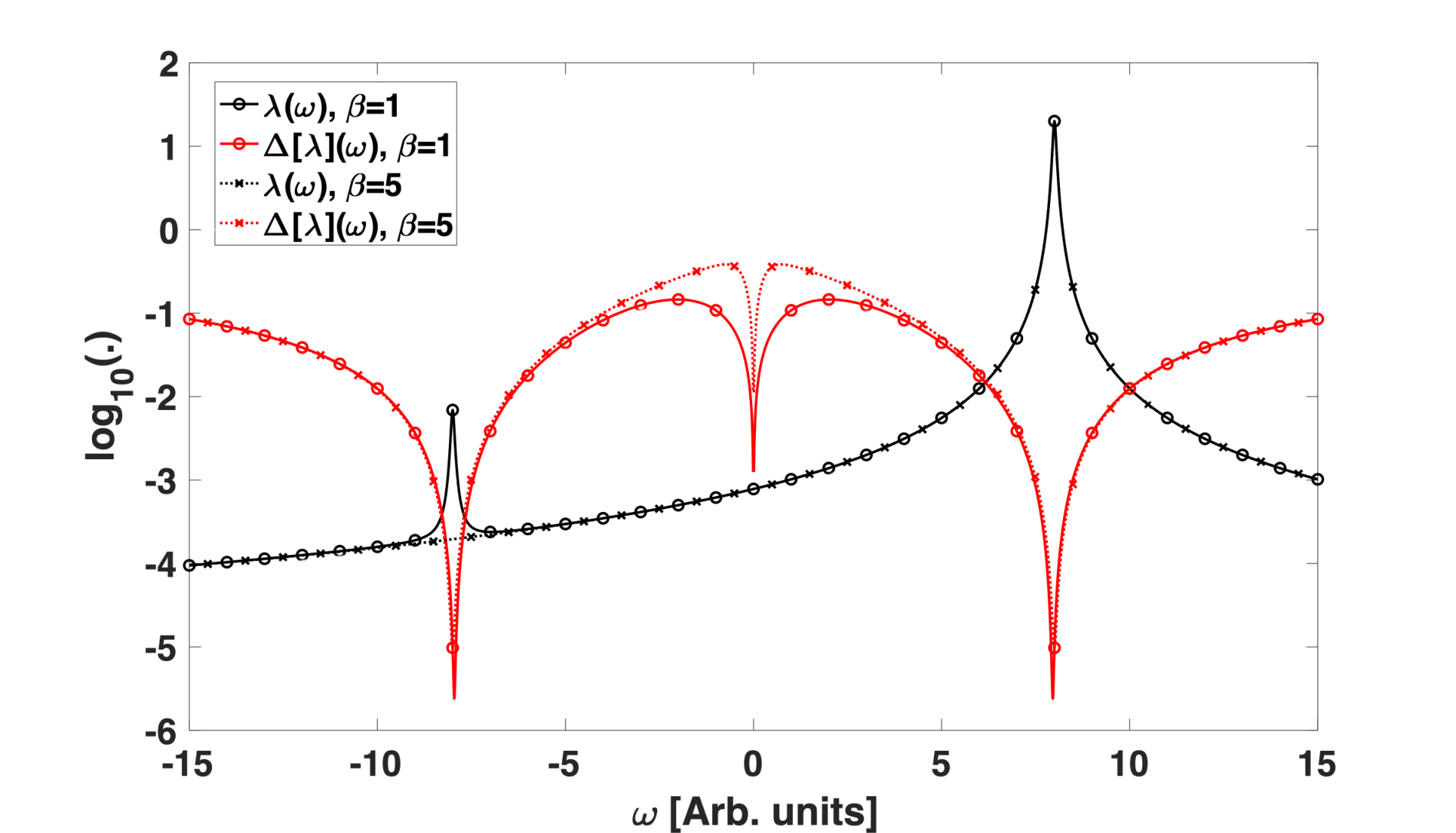
This metric helps us understand the detailed balance properties of the engineered transition rates for our protocol given in eq. 8. In fig. 2 we plot and as a function of for a fixed time for which . Two key points to note from this figure are: (i) as noted previously, the transition rates are significant only in a narrow range around , and (ii) violation of detailed balance is minimal at resonance () and at , and is significant only away from these regions. This is encouraging because it means that most of the eigenstate population redistribution will occur for transitions around resonance with , and in this region the detailed balance violation is small. Therefore, while the lack of detailed balance of our engineered rates will ultimately limit the thermalization performance, we expect that due to the properties highlighted above, the impact will be minimal in many cases.
It also helps to examine an explicit expression for , and some of its limiting properties:
From the limiting behavior we see that the detailed balance violation reduces for increasing temperature and for decreasing frequencies. Moreover, for decreasing temperature, the error metric limits to a saturating non-zero value, meaning that at low temperatures detailed balance violation will never be negligible, except possibly at resonance ().
Another interesting observation is the dependence of on . For fixed values of the other parameters, we see that decreasing decreases polynomially. However, due to the operating regime outlined in eq. 5, a decrease in should be accompanied by a decrease in the ancilla sweeping rate () and system-ancilla coupling strength (), meaning that the overall running time of the protocol increases.
It is worth elucidating the physical reason why yields higher quality thermalization; the ideal scenario from the system’s perspective is to “see” ancilla degrees of freedom at each instant in time with Boltzmann distributed populations and frequencies that are sharply resonant with transitions in . However, the entropy reduction mechanism that prepares the correct population distribution in the ancilla DOF, e.g., optical pumping, necessarily broadens the transition energies of the ancilla. Hence, achieving the ideal scenario of sharp resonances simultaneously with Boltzmann distributed populations is impossible with our protocol, and the best one can do is approximate this with .
Based on these observations about the behavior of the engineered spectral density that enters the dynamical master equation for the principal spins, we can surmise that the most challenging scenario for our protocol will be to thermalize to low temperature, , a system with energy gaps that are close to each other, but not degenerate and not close to zero. In this case the detailed balance violation at frequencies away from resonance – at the tails of the Lorentzian lineshape of the ancilla – is large, and due to the closely spaced gaps, there will be system transitions that lie on these tails. Therefore, while eigenstate population redistribution for transitions on resonance with the ancilla DOF (at any time) will mostly satisfy detailed balance, the non-zero spectral density away from resonance will drive nearby (in frequency) transitions, and the resulting population redistribution will violate detailed balance significantly. These conclusions will be illustrated in the numerical simulations in the next section and Appendix B.
V Potential Experimental Realization
In this section we evaluate the conclusions of the previous section through numerical simulation of the thermalization protocol on a small system that could also form the basis of a minimal experimental realization of the protocol.
We choose a system of two principal spins governed by the Hamiltonian
| (16) |
with variable parameters and . Each principal spin is coupled to an ancilla with the interaction
| (17) |
Note that we choose the system-ancilla coupling strength, , to be the same for both ancillae, and also choose the ancilla damping parameter and energy sweeping rates to be independent of (hence we drop the subscript on various quantities in the following). We choose a coupling to illustrate our scheme, but a or coupling scheme would be equally valid.
In the simulations below we use a piecewise linear (or sawtooth) sweep of the ancilla energies; i.e., over one cycle the modulation looks like with , and being the largest transition frequency for the system spectrum. The frequency is chosen so as to satisfy the parameter regime in eq. 5; i.e., .
In the following, we find it useful to vectorize the dynamical equation in eq. 6, and write
| (18) |
with
| (19) |
where is a vector whose elements are formed by stacking the columns of the density matrix, , and is the identity matrix of the same dimension as . We can formally solve this explicitly linear equation and write
| (20) |
where denotes time ordering.
We evaluate the steady-state of the dynamical system determined by our thermalization protocol by computing the first-order Trotter product approximation to the integrated map over a period
| (21) |
with . Since the dynamical generator in eq. 19 is periodic, the eigenvalue-zero eigenvector (the kernel solution) of this map over one period is the steady state of the engineered evolution. We denote this steady state as .
In order to assess the quality of thermalization we compute the trace distance between the density matrix at any time and the ideal thermal state, i.e., , with . The quality of thermalization of the steady state is then .
First, consider a fixed system Hamiltonian, given by and . The eigenstates of this Hamiltonian, in order of increasing energy are , , , , for real coefficients . To illustrate the thermalization dynamics we propagate the initial state according to the thermalizing master equation eq. 6, with , and the piecewise linear ancilla energy sweeps as mentioned above. fig. 3 shows the time development of eigenstate populations and the trace distance to the ideal thermal state under this evolution over a number of consecutive linear sweeps of ancilla energies over the range . We choose , which is a little over the maximum energy gap in the system. We show time evolution of the populations for two inverse temperatures, and . All populations monotonically converge to their ideal values for the given Hamiltonian, with at the end of the shown time evolution. Note that the changes in populations mostly occur in jumps over short time periods, and this is because most of the population mixing dynamics occurs during short periods when an ancilla DOF is in resonance with a system energy gap.
In Appendix B we present a thorough analysis of the thermalization performance in terms of the ancilla parameters, desired temperature, and the system Hamiltonian parameters. Although the construction of the thermalization protocol was mostly independent of the system Hamiltonian (except for the range of frequencies over which the ancilla are swept, which is set by the spectral range of ), we show that properties of the Hamiltonian subtly influence thermalization performance. In particular, the impact of the violation of detailed balance at intermediate and low temperatures can vary according to system Hamiltonian properties. To summarize the findings in Appendix B, the two cases where we find low thermalization performance are: (i) if the energy gaps in are congested in frequency (but not degenerate or close to zero), leading to off-resonant transitions driven by rates that significantly violate detailed balance, or (ii) at very low temperatures, if some ancilla-induced transitions are thermally suppressed, effectively hindering ergodicity (even though the system is formally ergodic).
Finally, in Appendix C we simulate the protocol and evaluate thermalization performance for larger systems, up to four principal spins.

V.1 Realistic parameters
In order to make the preceding numerical study more concrete we now map the parameters that determine the thermalizaton protocol to realistic values on several quantum simulation platforms.
In most quantum simulation and quantum computing platforms the most stringent restriction is the strength of achievable spin-spin couplings. We refer to this maximum achievable coupling strength as and choose since the system-ancilla coupling must be weaker than the couplings between principal spins. For example, in trapped ions coupling is typically achieved though the Mølmer-Sørenson interaction Sorensen and Molmer 1999; Sorensen and Molmer 2000; Milburn et al. 2000, whose strength depends on several factors including as trap geometry, but typical values are a few kHz (e.g., Refs. Kim et al. 2010; Gorman et al. 2018) and therefore for this platform we set kHz. Hence, kHz. So for example, in the simulations depicted in fig. 3 where we took , the units of time is s. Finally, a value of determines real thermalization target temperature on this platform through , and hence corresponds to K (K). Therefore, referring to fig. 3, we see that the thermalization protocol executed on the trapped ion platform enables generation of a thermal state of the two-spin system governed by Hamiltonian eq. 16 for values at temperature K (K) in time s (s).
We can similarly estimate the real temperatures corresponding to the simulations in fig. 3 and corresponding protocol running times for the superconducting qubit platform and the trapped neutral atom platform, and the results are presented in table 1. For the superconducting platform we use typical values of cross-resonance gate based couplings of MHz Sheldon et al. 2016; Chow et al. 2011 to fix MHz. For neutral atoms we assume spin-spin coupling through Rydberg interactions, and assuming a Rydberg blockade radius of 10 m, where the ratio of the Rydberg interaction to the ground-state interaction is large, we can fix the maximum coupling strength at MHz Saffman et al. 2010; Labuhn et al. 2016. In addition to the ability to engineer the system Hamiltonian and the system-ancilla couplings, our scheme requires an entropy reduction mechanism like optical pumping. Optical pumping or some variant of it are fairly routine on the neutral atom and trapped ion platforms, and similar mechanisms are also possible in superconducting circuits You and Nori 2011.
In all cases presented in table 1, the protocol runtimes are at the upper limit of typical quantum information protocol runtimes for the given experimental platforms. Hence decoherence mechanisms will impact dynamics, and may even be the dominant source of thermalization errors. Further analysis with particular decoherence models is necessary to understand the interplay between decoherence and the intrinsic open-system evolution engineered by our protocol, and how the former impact thermalization quality.
Finally, we note that the values presented in table 1 are only for one set of Hamiltonian parameters and for a particular choice for , and mainly serve to demonstrate that the thermalization protocol we have designed is realistic with existing technology. Given more precise estimates of experimentally feasible parameters and a desired , it is possible to do a more specific analysis of the achievable thermalization temperatures and runtimes.
| Platform | (MHz) | for | for | for | for |
|---|---|---|---|---|---|
| Trapped Ions | K | s | K | s | |
| Superconducting Qubits | mK | ms | K | ms | |
| Neutral Atoms | 22 2 Value extrapolated from exponential curve fit of experimental data Labuhn et al. 2016. | K | ms | K | ms |
VI Conclusions
Naive approaches to engineering thermalization in quantum simulators require either a coupling to a macroscopic harmonic reservoir or coupling to an extensive number of auxiliary states, each resonant with frequency transitions of the system eigenstates. Both of these approaches require a large number of ancillary DOF, and potentially also a detailed knowledge of the system spectra. In this work, we have developed an alternative approach to engineered thermalization with reduced resource counts by introducing a periodically driven and dissipated ancilla DOF, such that a single ancilla is resonant with different transitions at different times. This time-dependent approach merely requires an estimation of the full spectral width of the system Hamiltonian, and sufficient ancilla DOF to ensure ergodic system dynamics. Considering the interactions between the system and engineered ancilla DOF to be weak compared to interactions within the system, we derived a reduced description of the dissipative dynamics of the system that is in the form of a (time-dependent) Lindblad master equation. We then proved that the thermal state is the fixed point of the system evolution when a detailed balance condition is satisfied by the spectral density generated by the ancilla DOF, and also showed how violations of this condition impact thermalization performance.
Numerical investigations of a simple lattice system reveal the importance of parameter choices for generating thermal states using this protocol. In particular, the impact of detailed balance violation by our engineered “reservoir” varies according to the thermalization temperature and spectral properties of the system Hamiltonian. Thermalizing a many-body system using our protocol is most challenging when the system Hamiltonian has many gaps (transition energies) that are closely spaced (but not exactly degenerate or close to zero) and one demands thermalization to low temperatures. In this regime, the violation of detailed balance becomes most detrimental to thermalization performance. It is worth contrasting this with the thermalization of stabilizer Hamiltonians, which does not suffer from detailed balanced violation or increased thermalization time at low temperature because the system gaps (and thus ancilla energies) are constant and known Young et al. 2012; Herdman et al. 2010. Numerical investigations also revealed an interesting obstruction to thermalization at low temperatures; a type of degradation of ergodicity due to suppression of certain transitions from lack of thermal energy.
We have developed this thermalization protocol in the framework of continuous-time dynamics. In future work, we will investigate what a discrete-time, or gate-based, version of such a time-dependent ancilla-driven thermalization protocol looks like (cf. the spectral combing protocol in Ref. Kaplan et al. 2017). In particular, we are interested in whether a gate-based version of such a thermalization protocol enables one to overcome the fundamental limitation we identified in the continuous-time protocol; namely, that the entropy reduction mechanism that prepares the correct population distribution in the ancilla DOF also broadens the transition energies of the ancilla, and results in driving of off-resonant transitions at rates that violate of detailed balance. Besides, the formulation of a gate-based version of our protocol would enable rigorous comparison to well-established gate-based thermalization protocols, e.g., Ref. Temme et al. 2011.
Acknowledgements.
Sandia National Laboratories is a multimission laboratory managed and operated by National Technology & Engineering Solutions of Sandia, LLC, a wholly owned subsidiary of Honeywell International Inc., for the U.S. Department of Energy’s National Nuclear Security Administration under contract DE-NA0003525. This paper describes objective technical results and analysis. Any subjective views or opinions that might be expressed in the paper do not necessarily represent the views of the U.S. Department of Energy or the United States Government. This material is based upon work supported by the U.S. Department of Energy, Office of Science, Office of Advanced Scientific Computing Research, under the Quantum Computing Application Teams and Quantum Algorithm Teams programs.References
- Brandao and Svore (2016) Fernando G. S. L. Brandao and Krysta Svore, “Quantum Speed-ups for Semidefinite Programming,” arXiv:1609.05537 [quant-ph] (2016).
- Kliesch et al. (2011) M. Kliesch, T. Barthel, C. Gogolin, M. Kastoryano, and J. Eisert, “Dissipative quantum church-turing theorem,” Phys. Rev. Lett. 107, 120501 (2011).
- Riera et al. (2012) Arnau Riera, Christian Gogolin, and Jens Eisert, “Thermalization in nature and on a quantum computer,” Phys. Rev. Lett. 108, 080402 (2012).
- Binder and Heermann (2010) Kurt Binder and Dieter Heermann, Monte Carlo Simulation in Statistical Physics - An Introduction | Kurt Binder | Springer, 5th ed. (Springer, 2010).
- Landau and Binder (2014) David P. Landau and Kurt Binder, A Guide to Monte Carlo Simulations in Statistical Physics (Cambridge University Press, 2014).
- Pang (2016) Tao Pang, An Introduction to Quantum Monte Carlo Methods (Morgan & Claypool Publishers, 2016).
- Georgescu et al. (2014) I.M. Georgescu, S. Ashhab, and Franco Nori, “Quantum simulation,” Rev. Mod. Phys. 86, 153 (2014).
- Gross and Bloch (2017) Christian Gross and Immanuel Bloch, “Quantum simulations with ultracold atoms in optical lattices,” Science 357, 995–1001 (2017).
- Metcalf et al. (2016) M. Metcalf, C.Y. Lai, and C.C. Chien, “Hysteresis of noninteracting and spin-orbit-couples atomic fermi gases with relaxation,” Phys. Rev. A 93, 053617 (2016).
- Kaplan et al. (2017) David B. Kaplan, Natalie Klco, and Alessandro Roggero, “Ground States via Spectral Combing on a Quantum Computer,” arXiv: 1709.08250 [quant-ph] (2017).
- Polla et al. (2019) Stefano Polla, Yaroslav Herasymenko, and Thomas E. O’Brien, “Quantum digital cooling,” arXiv:1909.10538 (2019).
- Herdman et al. (2010) C. M. Herdman, Kevin C. Young, V W Scarola, Mohan Sarovar, and K. B. Whaley, “Stroboscopic generation of topological protection,” Physical Review Letters 104, 230501 (2010).
- Young et al. (2012) K. C. Young, M. Sarovar, J. Aytac, C. M. Herdman, and K. B. Whaley, “Finite temperature quantum simulation of stabilizer Hamiltonians,” J. Phys. B: At. Mol. Opt. Phys. 45, 154012 (2012).
- Kitaev and Laumann (2009) Alexei Kitaev and Chris Laumann, “Topological phases and quantum computation,” arXiv: 0904.2771 [cond-mat] (2009).
- Shabani and Neven (2016) Alireza Shabani and Hartmut Neven, “Artificial quantum thermal bath: Engineering temperature for a many-body quantum system,” Phys. Rev. A 94, 052301 (2016).
- Kempe et al. (2006) Julia Kempe, Alexei Kitaev, and Oded Regev, “The complexity of the local Hamiltonian problem,” SIAM J. Comp. 35, 1070 (2006).
- Aharonov et al. (2009) Dorit Aharonov, Daniel Gottesman, Sandy Irani, and Julia Kempe, “The power of quantum systems on a line,” Communications in Mathematical Physics 287, 41–65 (2009), arXiv: 0705.4077.
- Anschuetz and Cao (2019) Eric R. Anschuetz and Yudong Cao, “Realizing quantum boltzmann machines through eigenstate thermalization,” arXive: 1903.01359 (2019).
- Steck (2013) Daniel A Steck, “Quantum and Atom Optics,” (2013).
- Breuer and Petruccione (2002) H-P Breuer and F Petruccione, The theory of open quantum systems, Book (Springer, 2002).
- (21) This property relies on the system operator of the system-bath coupling ( in eq. 1) being Hermitian. However, this derivation can be generalized to cases where the coupling is not Hermitian also.
- Sorensen and Molmer (1999) A Sorensen and K. Molmer, “Quantum Computation with Ions in Thermal Motion,” Phys. Rev. Lett. 82, 1971 (1999).
- Sorensen and Molmer (2000) Anders S Sorensen and Klaus Molmer, “Entanglement and quantum computation with ions in thermal motion,” Phys. Rev. A 62, 22311 (2000).
- Milburn et al. (2000) G J Milburn, S Schneider, and D F V James, “Ion Trap Quantum Computing with Warm Ions,” Fortschr. Phys. , 10 (2000).
- Kim et al. (2010) K. Kim, M S Chang, S Korenblit, R Islam, E E Edwards, J K Freericks, G-D Lin, L-M Duan, and C Monroe, “Quantum simulation of frustrated Ising spins with trapped ions,” Nature 465, 590–593 (2010).
- Gorman et al. (2018) Dylan J Gorman, Boerge Hemmerling, Eli Megidish, Soenke A Moeller, Philipp Schindler, Mohan Sarovar, and Hartmut Haeffner, “Engineering Vibrationally Assisted Energy Transfer in a Trapped-Ion Quantum Simulator,” Phys. Rev. X 8, 011038 (2018).
- Sheldon et al. (2016) Sarah Sheldon, Easwar Magesan, Jerry M. Chow, and Jay M. Gambetta, “Procedure for systematically tuning up cross-talk in the cross-resonance gate,” Phys. Rev. A 93, 060302(R) (2016).
- Chow et al. (2011) Jerry M. Chow, A. D. Corcoles, Jay M. Gambetta, Chad Rigetti, B. R. Johnson, John A. Smolin, J. R. Rozen, George A. Keefe, Mary B. Rothwell, Mark B. Ketchen, and M. Steffen, “Simple all-microwave entangling gate for fixed-frequency superconducting qubits,” Phys. Rev. Lett. 107, 080502 (2011).
- Saffman et al. (2010) M. Saffman, T. G. Walker, and K. Mølmer, “Quantum information with rydberg atoms,” Rev. Mod. Phys. 82, 2313 (2010).
- Labuhn et al. (2016) Henning Labuhn, Daniel Barredo, Sylvain Ravets, Sylvain de Léséleuc, Tommaso Macrì, Thierry Lahaye, and Antoine Browaeys, “Tunable two-dimensional arrays of single rydberg atoms for realizing quantum ising models,” Nature 534, 667–670 (2016).
- You and Nori (2011) J. Q. You and Franco Nori, “Atomic physics and quantum optics using superconducting circuits,” Nature 474, 589–597 (2011).
- Temme et al. (2011) K Temme, T J Osborne, K G Vollbrecht, and D Poulin, “Quantum metropolis sampling,” Nature 471, 87–90 (2011).
- Kołodyński et al. (2018) Jan Kołodyński, Jonatan Bohr Brask, Martí Perarnau-Llobet, and Bogna Bylicka, “Adding dynamical generators in quantum master equations,” Physical Review A 97, 062124 (2018).
Appendix A Derivation of reduced master equation for principal spin lattice
As described in the main text, physical motivations led to a choice of parameter regime for the thermalization protocol:
| (22) |
The dynamics of the system (principal spins defining the many-body model and the ancilla spins) are governed by the Hamiltonian in eq. 1 and the dissipative evolution of ancilla spins given in eq. 3. Define as the density matrix for the combined system and ancilla spins – i.e., , the space of positive, trace one operators on the combined Hilbert space. Further, let be the reduced density operator for the system ( denotes a trace over the ancilla subsystem).
We will derive a reduced master equation for assuming one ancilla spin (). The result generalizes immediately since each ancilla is weakly coupled and is independent of all other ancilla, and hence additivity of Lindblad evolutions applies Kołodyński et al. 2018. In the following, we will follow the standard derivation of a master equation in the Born and Markov approximations, but we need to justify some of the steps carefully in this context since instead of a macroscopic reservoir we have a damped and driven ancilla spin.
In the interaction picture (with respect to the free evolution of the system and ancilla) the evolution of the combined system is
| (23) |
for some spin in the system, , and where the tilde denotes operators in the interaction picture. Following the standard derivation Breuer and Petruccione 2002, by iterating this equation and formally integrating we get
| (24) |
At this point we make three approximations. First, we replace with , with the justification being that in the weak coupling limit, any entanglement between system and ancilla is quickly damped by the ancilla dynamics and hence we can replace the joint state with a tensor product state. Moreover, the state of the ancilla will can be approximated by an equilibrium state , which we will take later to be the thermal state with respect to some and the transition energy at time , . Note that in standard derivations of the Born-Markov master equation, this state is taken to be time-independent, whereas since we need to sweep the ancilla energy, we keep the time-dependence on the “reservoir” state. The second approximation is that we will replace with , with the justification that the trace over the ancilla degrees of freedom will yield a correlation function that decays rapidly as , and hence only the values of the integral around really contribute. Finally, we take the upper limit of the integral , again using the approximation that the correlation function decays rapidly and so integrand values at large values of are negligible. With these approximations we get:
| (25) |
Now let us examine the form of more closely. We first define a frequency resolved operator on the system
| (26) |
where is a projector on the eigenspace of with eigenvalue . Using this definition, the following properties are easy to prove:
| (27) |
Using these properties, we expand eq. 25 as:
| (28) |
with
| (29) |
Assume that over sufficiently long times (since we are mostly concerned about steady state properties long times are of primary interest) the oscillating factor damps any terms with . Dropping these terms (which amounts to the secular, or rotating wave, approximation), we get:
| (30) |
Now let us examine the Fourier transforms of the reservoir correlation function, eq. 29. As is customary in the derivation of a Lindblad master equation we assume that the correlation functions are homogeneous in time. This follows easily for large reservoirs near equilibrium but needs more careful thought in our case where we have a driven, dissipated ancilla spin. Since the ancilla energies are periodic there is clearly some non-homogeneity to the correlation function. However, since the change in energy is much slower than the system-reservoir coupling and the ancilla damping we assume that on timescales resolved by the interaction the homogeneity of the correlation function is a valid assumption.
Given time-homogeneity of the correlation function we rewrite as
| (31) |
To evaluate this quantity, we need to know time dynamics of the operator . These dynamics are dominated by the driving and dissipation of the ancilla spins, and hence we calculate the correlation functions by formulating the adjoint version of the ancilla dynamics from its free Hamiltonian and the master equation in eq. 3
| (32) |
where is any operator acting on , and . According to this adjoint evolution equation,
| (33) |
where . In the quasi-static limit where we ignore the time-dependence of and , we can solve these equations easily and get
| (34) |
Finally, since is a Gibbs state and hence diagonal in the computational basis, we get
| (35) |
where and are the Boltzmann distributed populations of the ancilla spin.
At this point, we have a Markov master equation (with time-dependent coefficients) describing the evolution of the system alone (in the interaction picture). To further isolate the dynamics of interest, we separate out the Lamb shift resulting from the coupling to the reservoir from the incoherent dynamics. To do this, we separate the real and imaginary components of eq. 35, as . The Lamb shift Hamiltonian is then Breuer and Petruccione 2002
| (36) |
Owing to the properties in eq. 27, we know , and therefore for the purposes of preparing thermal states of the system, the Lamb shift is inconsequential. It will shift some of the system energies around, however, since our protocol does not require precise knowledge of the system energies this is not important. So we ignore it from now on. The real part of , on the other hand, yields the incoherent dynamics that we want to tune to achieve thermalization of the system. Explicitly, the real part is:
| (37) |
To summarize, we write the relevant dynamics of the system alone, in the interaction frame with respect to as:
| (38) |
In the general case where we have many ancilla spins, one simply has a sum of the above Lindblad evolution for each system-ancilla coupling.
Appendix B Thermal state accuracy as a function of parameters
In this Appendix we study the accuracy of thermal state preparation for the two-spin principal system studied in the main text, as a function of the protocol’s and system’s parameters.
First, we study the behavior as a function of the engineered bath parameters; the ancilla damping rate, , and the desired inverse temperature, . fig. 4 shows the trace distance between the steady-state and the ideal thermal state as a function of these parameters, with the Hamiltonian parameters fixed at . For each point, we choose the other parameters consistent with the regime in eq. 5 – i.e., and . We see that the protocol is able to prepare states that are very close to the true thermal state. The poorest performance is in the region where is too large or the desired temperature is too low, but even here the trace distance to the ideal thermal state is close to . The region of poorest performance is consistent with our analysis in the main text that showed that the violation of detailed balance increases when or increase.

Next, we study thermalization performance as a function of the parameters and in . Although the construction of the thermalization protocol was mostly independent of the system Hamiltonian (except for the range of frequencies over which the ancilla are swept, which is set by the spectral range of ), we will see that properties of the Hamiltonian subtly influence thermalization performance. In particular, we show how the impact of the violation of detailed balance at intermediate and low temperatures can vary according to system Hamiltonian properties.

In fig. 5 (a) and (b) we show, as a function of the parameters and , the spectrum of and the connectivity of the eigenstates of , respectively. From fig. 5 (a) we see that the spectrum varies in a complicated manner across this parameter regime – importantly, in the region , the spectrum becomes congested, with even several points of degeneracy between states and , and also and (we will label the eigenstates of , in order of increasing energy, as , and gaps as ). The connectivity of the eigenstates can mostly be classified into three types, depending on the region in parameter space. In fig. 5 (b) we show these three regions, labeled R1, R2, R3, and how the eigenstates of are connected there – a red arrow between the states separated by , indicates that is non-zero for , , or both. fig. 5 (b) shows that while the system is ergodic for all values of , the direct connectivity of eigenstates varies, and this will play an important role in thermalization quality. Finally, in fig. 5(c) we summarize how the spread in transition energies varies for the Hamiltonian parameters by plotting the interquartile range (IQR) for energies of the allowed transitions at each . We choose IQR to represent the spread of gaps because it is less sensitive to outliers (there is one large gap at most parameter values) than other measures of deviation.
To summarize thermalization behavior, in fig. 6 we show the trace distance between the ideal thermal state and the steady state of the engineered evolution for intermediate and low temperatures, as a function of the Hamiltonian parameters . The values of the other parameters for all of these plots are , and as before, we used a linear sweep of the ancilla energies over the range , where is the maximum gap in the Hamiltonian energies for the chosen . The linear sweep duration is set by . We restrict to positive values of because the thermalization performance is symmetric about .
In the intermediate temperature case, fig. 6(a), we see that the trace distance is below across the whole parameter range. The worst performance is in a wide region in the center of the parameter space, and by comparing fig. 6(a) to fig. 5(c) we see that this region corresponds to the region with the smallest spread in gaps in the system. Therefore we conclude that the poorer performance in this region is due to the effect identified in section IV. Namely, when there are closely spaced gaps, off-resonant transitions can be driven by rates that significantly violate detailed balance, because as shown in fig. 2 around the tails of the instantaneous Lorentzian spectral density, transition rates are non-negligible and there is significant detailed balance violation at once. Note that in the region , the thermalization performance is better even though the gaps are very congested here also. The reason is that the two most important gaps at this temperature, and , are almost zero and almost degenerate in this region (see fig. 5(a)), and thus the detailed balance violation is softened here (recall that decreases around , and moreover, if two gaps are almost degenerate, then although one may drive the off-resonant transition, it will be close enough to resonance that the violation of detailed balance is minimal).

Moving onto the low temperature case, fig. 6(b), we see that the trace distances are uniformly greater than the intermediate temperature case. This is consistent with our previous observation that the effectiveness of the thermalization protocol degrades as the target temperature reduces. Despite this, the achieved trace distance at low temperature () over most of the Hamiltonian parameter space is fairly small (). The exception to this is in part of region R1, with and . To explain the deviation we return to fig. 5 (b), where we showed that in region R1 states and are not directly connected by an ancilla-induced transition. At the majority of the population of the ideal thermal state in this region is distributed between states and , however, if these states are not directly connected, in order to distribute population between these states, one needs to go through transitions to higher energy states. But such transitions are highly suppressed at low temperatures because the thermal energy provided by the ancilla DOFs is too small; i.e., for . This accounts for the large trace distance between the steady state and the ideal thermal state in this parameter region of the Hamiltonian at low temperature. This example demonstrates that even if a system is formally ergodic, ideal thermalization can be prevented if all transitions are not thermally activated.
Appendix C Evaluating thermalization quality for larger system sizes

We evaluate the effectiveness of our protocol numerically by determining the fixed point of evolution for a spin chain with pair-wise interactions with increasing length. The Hamiltonian defines a system with alternating onsite energies and interactions between the X, Y and Z spin degrees of freedom,
| (39) |
Numerically, we build the generator in Equation 19 and the kernel solution by diagonalizing the time-ordered linear map within Equation 21 which is equivalent to the steady-state solution . Coupling alternating principal spins to an ancilla spin, for even L and for odd L, on the spin chain has a unique steady state solution approximating the thermal state and reduces computational resources required for exact numerical simulation. We compute the trace distance between the steady-state solution from the true thermal state for a one-dimensional spin chain with and at varied temperatures Fig. 7. It is evident the steady-state remains a good approximation of the true thermal state with increasing system size at low, high and intermediate temperatures.
In the numerical algorithm we store the entirety of Equation 19 in memory to reduce the computational complexity in time, and the amount of memory bytes required to construct Equation 19 scales where M is the total number of ancilla spins, is the number of unique system frequencies, and L is the length of the spin chain. The computational overhead limits exact numerical simulation to small spin chains, however the generator is sparse and sparse linear algebra computations can reduce memory requirements. Moreover, as shown in Eq. 14 in the main text, one could simplify further by just simulating population dynamics. However, in this work we limit ourselves to small-scale simulations designed to demonstrate the basics of the protocol, and do not pursue simulations of large-scale systems.