Exact non-symmetric closed line vacuum magnetic fields in a topological torusPreprint: AIP/123-QED
Abstract
Non-symmetric vacuum magnetic fields with closed magnetic field lines are of interest in the construction of stellarator equilibria. Beyond the result of D.Lortz (ZAMP 21, 196 (1970)), few results are available. This work presents a closed-form expression for a class of vacuum magnetic fields in a topological torus with closed field lines. We explicitly obtain the invariants of such a field. We finally show that a three-dimensional low beta magnetohydrodynamic (MHD) equilibrium may be constructed in a topological torus, starting with these closed line vacuum magnetic fields.
Keywords:
closed line, non-symmetric, three-dimensional, vacuum magnetic fields, exact solutionI Introduction
The existence of magnetic fields for non-dissipative plasma models in a multiply connected domain with nested flux surfaces or exclusively closed field lines remains an incompletely understood topic. While the existence of magnetic surfaces is easily demonstrated in domains with continuous symmetry such as toroidal, cylindrical, helical, or translational, it is well understood that such surfaces are easily destroyed by small perturbations that destroy the original symmetry. In particular, if we look for continuously deformable smooth and continuous non-symmetric solutions of ideal MHD, the pressure and rotation transform profiles cannot be arbitrarily chosen to avoid the singular divisors on rational surfaces (Grad 1967; Newcomb 1959; Hudson and Kraus 2017).
To avoid magnetic resonances, modern stellarators like W7-X and HSX are designed to have low global magnetic shear. The behavior of low-shear magnetic field systems can be markedly different in the neighborhood of closed field lines from generic ergodic surfaces (Firpo and Constantinescu 2011; Faber et al. 2018). Numerous experimental results from Wendelstein VII-A/AS (Hirsch et al. 2008; Brakel and the W7-AS Team 2002; Brakel et al. 1997) and numerical results (Wobig 1987; Andreeva 2002) support the idea that optimum confinement is usually found close to certain low-order rational surfaces. For small but arbitrary perturbations, the islands on these surfaces are found (Wobig 1987) to be exponentially small in size consistent with Arnold’s theorem on “properly degenerate systems.” The stability advantages of low-shear MHD systems compared to the high shear systems have also been discussed (Grad 1973; Strauss and Monticello 1981). W7-X has two very different configurations, which both access regions close to , namely, the standard configuration and the high-- configuration (Andreeva 2002; Klinger et al. 2019). In the former case, shear is relatively large compared to the latter, and there are islands near in the former but not in the latter. Therefore, it is indeed possible to have low-shear regions near low-order rational surfaces under experimental conditions, but careful design is needed (Lazerson et al. 2019).
The possibility of the existence of nested surfaces or closed field lines in generic three-dimensional domains is an open mathematical question with at least one notable example of an ideal magnetohydrodynamic equilibrium in a non-symmetric domain as given by D.Lortz Lortz 1970. Lortz showed that in a system with reflection symmetry, a non-symmetric three-dimensional MHD equilibrium with a smooth pressure profile can be constructed iteratively starting with a vacuum field which has closed field lines and zero shear. A significant drawback of this result is that the rotation transform for such an equilibrium is zero.
The difficulties in obtaining exact solutions or even perturbative analytic expressions for three-dimensional non-symmetric vacuum magnetic fields with surfaces have been pointed out (Cary 1982; Freidberg 1982; Sengupta and Weitzner 2018). For ideal magnetohydrodynamics, the literature has a rich collection of formal expressions of equilibria, expansions being in the amplitude of magnetic field components Weitzner 2014; Cary 1984 or in the distance from a magnetic axis Mercier 1964; Solov’ev and Shafranov 1970, a magnetic line or a magnetic surface Weitzner 2016; Sengupta and Weitzner 2019. Some of these expansions are shown to be able to be carried to all orders; many are carried out only to the first few orders. The convergence of these series expansions is not known, nor is their non-convergence. In an earlier paper Sengupta and Weitzner 2019, we treated the formally simple problem of the expansion of a vacuum magnetic field, the expansion being in the distance of a planar surface, say . The magnetic field was found to be periodic of period in the two orthogonal coordinates and . Such periodicity renders the domain of definition of the magnetic field doubly connected, i.e., a “torus. ” We developed expansions to all orders in the distance from the plane . The ability to expand to all orders, at least as we carried it out, severely limited the possible magnetic fields. We do not know if these limitations are real or a consequence of our approach to the problem. We did not examine the convergence of the series, either.
In this work, we return to the problem previously studied and extend the analysis further. In section II, we take the magnetic field structure used there, we extend the scalar potential for the vacuum field to an explicit representation in all space, and finally show that in some open set containing the plane every magnetic field line is closed. We comment on a few properties of such fields. The representation of allows either finite or infinite series representations. We omit the restrictions necessary in the latter case. In section III, we treat one particularly simple representation of a closed line system in greater detail and obtain the Clebsch potentials. In section IV, we show that the Lortz analysis allows this special vacuum field to be the starting point for the expansion in power series of plasma beta . We discuss how the Lortz iteration scheme allows us to construct non-symmetric MHD equilibrium with closed field lines. We require only a minimal result from the earlier work.
II Construction of a vacuum magnetic field with closed field lines
Since is a vacuum magnetic field, we introduce a scalar potential , such that
| (1) |
We assume that is an even function of and that on the plane ,
| (2) |
Here is an odd function of of the form
| (3) |
where is periodic of period in and is a constant. We found Sengupta and Weitzner 2019 for such fields that one could find magnetic surfaces to all orders. The properties that be even in , a solution of Laplace’s equation and the form (2) completely characterizes and we obtain
| (4) |
If we then use the structure and parity of we conclude that
or,
| (5) |
We conclude immediately from the form (5) that the coefficients must be severely constrained so that the series represents an analytic function of in some domain . Such conditions are lost in the formal series analysis used previously. For simplicity we assume here that at most a finite number of coefficients are non-zero and that the parameter is small enough such that
| (6) |
We could extend the analysis to allow infinitely non-zero values of , provided more stringent inequalities of the form (6) were imposed. With as given by (5) satisfying (6), we now show that every magnetic field line in some region is closed.
We observe that a magnetic field line satisfies the equation
| (7) |
It is convenient to change the independent coordinates from to where
| (8a) | ||||
| (8b) | ||||
| (8c) | ||||
The transformation (8) is a rotation of about the axis followed by a stretching of all coordinates by a factor . Clearly, we may follow magnetic field lines in either coordinates to demonstrate closure, as the relation (7) is only modified by a coordinate stretching. We find easily that
| (9) |
Thus, the equations for a magnetic field line are
| (10a) | ||||
| (10b) | ||||
| (10c) | ||||
We note that there is a unique magnetic field through any given point . Further, the field line is an analytic function of the initial values, so that in any bounded domain the field is a uniformly continuous function of the initial data. Next we observe that any field line through remains in the plane. Equally, every field line through the plane, remains in that plane for every integer . Finally, we conclude that there is an open set containing the section of the plane with such that
| (11) |
and every field line remains in that domain. In view of (10b), is a monotonic increasing function of . We may therefore write the equations in the form
| (12a) | ||||
| (12b) | ||||
| (12c) | ||||
If we change the independent variables from to , then as ranges from 0 to , ranges from to and back to . Since, and , the field line is closed.
The closure of the field lines found here for the field with scalar potential depends on the reflection symmetry that be even in and odd in , essentially the same discrete symmetry used by Lortz. We append a standard but rarely discussed result for our system: that the rotational transform of a closed line magnetic field is not well defined. We start from the field as given by (11,12). We may generalize the transformation 8 to
| (13a) | ||||
| (13b) | ||||
| (13c) | ||||
where are relatively prime. Again, (13) is a rotation about the axis by an angle of followed by a stretch. Thus, again, the field lines are periodic of period in . The field line starting at after one period , has . Correspondingly, the two points are and . Hence, the field lines will have a twist of or . Usually, one identifies the twist with the rotational transform, but clearly, the identification here is spurious. Thus, the concept of a rotation transform, in this case, is ill-defined.
Finally, we note that while periodicity in the expression for in the variable is essential, the specific form for as a function of is not. Thus, each term might be replaced by , and the subsequent analysis would be possible with only minor modifications at each step. These modifications allow a more extensive range of vacuum fields and of equilibria than are shown explicitly.
III Clebsch representation for the vacuum magnetic field
It is useful to explore a simple, explicit version of these results. To that end we set for all i.e.
| (14) |
where . We shall now construct explicitly such that
| (15) |
using method of characteristics. We solve
| (16) | ||||
We observe that the equations are invariant under
| (17) |
Hence, the invariants must be even functions of all the coordinates. Since and vanish at and respectively, the characteristics have to be calculated separately on the and planes and for regions. We now discuss each of these regions separately.
III.0.1 Invariants on the plane
Substituting in (16) we obtain
| (18) |
Since vanishes at , field lines do not cross the plane. Therefore, we treat and regions separately. For , we can easily integrate (18) subject to parity condition (17) and obtain
| (19) |
where, is a constant along the field lines. Thus, and constant, are the two invariants in this case. We note that for small , and that (19) shows is singular at .
III.0.2 Invariants on the plane
III.0.3 Invariants when
Finally, when , it is easily verified that the following two functions are constants along any magnetic field satisfying (16) together with (17):
| (22a) | ||||
| (22b) | ||||
where,
| (23) |
In obtaining the above we have made use of the identity
| (24) |
which follows from the form of the invariant . We note several important features of the functions and . The functions satisfy the parity condition (17) but are not analytic everywhere. The function is not analytic near while is not analytic near and . The lower limit on the integral ensures that is continuous across where is discontinuous. It can be easily verified that (15) is satisfied when . The integrals appearing in (21,22) can be evaluated explicitly in terms of incomplete elliptic integral of the first kind.


The contours of constant , as shown in figure (1(a)) and (2), forms nested surfaces separated by the and planes and has a X-point at . Remarkably, is independent of both the coordinate and the aspect ratio parameter for this class of fields. The other Clebsch variable, , is manifestly three-dimensional, as shown in figure 3.
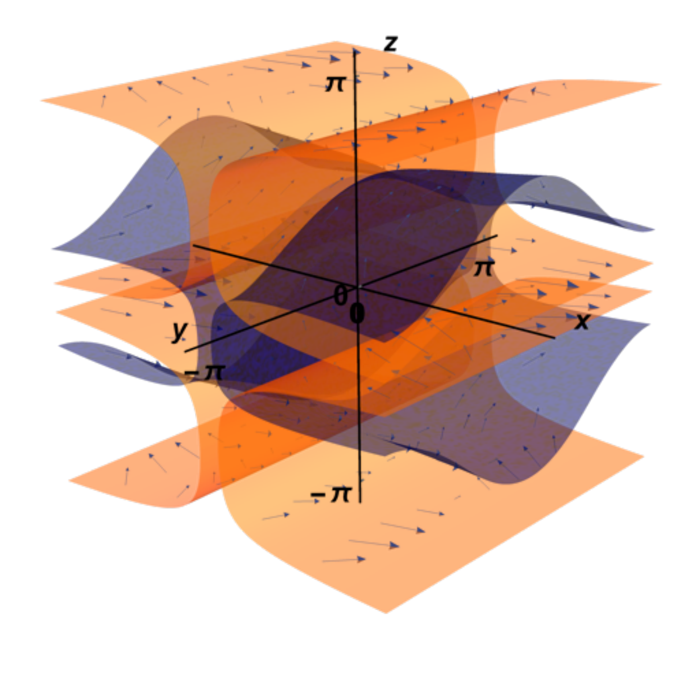
Near the plane and arbitrary and ,
| (25) | ||||
Both and approach zero as approaches zero but the magnetic field given by is nonzero.
Since there is a gauge degree of freedom in choosing the Clebsch potentials such that is unchanged, we can choose and as new Clebsch potential. From 25, we find that has second harmonics in (poloidal) angle and the hyperbolic dependence on as expected from near-axis expansions Solov’ev and Shafranov 1970.
On the other hand when we approach the plane, and and are arbitrary,
| (26) |
Near the X-point where both and approach zero
| (27) |
In addition to the possible value of explicit examples of doubly periodic vacuum magnetic fields with closed field lines, the results also provide an indirect validation of the formal expansion for vacuum magnetic field flux surface.
IV The Lortz construction of ideal MHD equilibrium
We next apply the Lortz construction of an ideal MHD toroidal equilibrium as a convergent power series expansion in the parameter beta, starting from a given closed line vacuum magnetic field. Magnetic field line closure is guaranteed order by order in the expansion by the condition that the magnetic fields have reflection symmetry in a given plane. In the present case, the torus is defined by the two “angles” and , and the system is periodic in each of the angles. The system will be designed to be symmetric on reflection in the plane , so is an even function of , and the other two components are odd in . The domain is defined by the relation
| (28) |
We discuss the nature of and after further elaboration. We finally obtain equilibrium with boundaries, which are also constant pressure surfaces and with interior pressure maximum or a unique pressure maximum. Neither of these properties holds for the original Lortz analysis. We choose the vacuum field with . We restrict the magnitude of in the subsequent analysis.
The Lortz analysis is based on the equilibrium representation
| (29a) | ||||
| (29b) | ||||
| (29c) | ||||
| (29d) | ||||
The integral for is along a field line starting on some fixed plane in the domain of interest. We follow the Lortz notation and note that is not the standard tokamak safety factor. We recall that we start with a given closed line magnetic field, evaluate and then determine a new closed line magnetic field and then iterate. The details are as follows:
- 1.
After iterations, we calculate and from .
- 2.
With known, we update pressure where, the specific form of pressure is an arbitrary input.
- 3.
From pressure and , we update currents using .
- 4.
Using , we update and then iterate.
Provided is sufficiently small and provided each iterate has reflection symmetry in the plane the process converges. The additional currents due to finite pressure do not create islands as they are incorporated self-consistently in the pressure profile in each iteration. The periods in and and hence the rotation transform stay fixed. Closed magnetic field lines, therefore, remain closed even with the addition of pressure and currents.
IV.1 Calculation of q
It is clear from the preceding discussion that the properties of and especially of for the initial vacuum field are critical to start the analysis, and we explore the properties of for our chosen vacuum field. A magnetic field line is given by the solution of the equations
| (30a) | ||||
| (30b) | ||||
| (30c) | ||||
and
| (31) |
It is convenient to re-express (30) in terms of . We note that in the range , covers the values from -1 to +1 with increasing with negative, while in the range , is decreasing with positive. Thus, we find
| (32) |
In the form (32) and using (30) it is relatively straightforward to obtain the needed properties of .
We study the system (30,31) for small and we see that
| (33a) | ||||
| (33b) | ||||
We obtain readily
| (34) |
The critical points of the function that occur at are saddle points. To analyze the behavior of near and arbitrary , we must expand further. We set and find
| (35) |
so that is a center.
We show the variation of with the invariant and in figure 4. The function is bounded from above by which is the value of when both and are zero, i.e., at the X-point. On the other hand, at the centers (), , as can be seen from (32).
The expansion is seen to be in excellent agreement with the numerically obtained value of . Figure 5 show the results of the expansion carried to fourth-order. The analytical expressions for various quantities are provided in the appendix. The saddle point at () and the center at () are clearly visible. We see from (34) and (35) that a class of curves constant, is approximately given by constant. In particular, the lines
| (36) |
approximate the separatrix joining the saddle point to .

We observe that for large , the contours bunch around a boundary, which is shown in the appendix to be the curve . From the definition of (32), we see that the perturbation theory can fail for large as approaches zero. Physically, the magnetic field has a turning point near this boundary, and therefore, can become singular. We present a detailed description of the behavior of near this boundary in the appendix. We show that , in general, has a logarithmic divergence near the boundary . As a concrete demonstration of the logarithmic behavior near the boundary, we calculate analytically the value of for large without the expansion. Figure 6 compares the exact expression for for large (53) to the result obtained using the expansion. As seen from the figure, near the boundary , which occurs when , diverges logarithmically. The curve is indeed the boundary on which vanishes.
Finally, we observe that any sufficiently small and sufficiently smooth perturbation of cannot change the character of . There remain centers in the neighborhood of (). Thus, one might add additional sufficiently small terms from the series (9). Hence, the behavior of presented here is expected to be modified only slightly when plasma is introduced as a small perturbation to the vacuum magnetic field system in the Lortz iteration scheme.
IV.2 Lortz iteration
We now restate the critical elements of the Lortz iteration. We solve Eq.(29) iteratively. The solution of the system is to have reflection symmetry in some planes. That symmetry may be translated into even and odd conditions in the components of on the given plane. If the domain is multiply connected, then appropriate periods must be given. Provided the domain boundary and the function is sufficiently smooth, and provided there is a vacuum field satisfying all the periodicity, periods and symmetry conditions, then for sufficiently small, a solution of system (29) exists with appropriate smoothness properties. The iteration starts with , and from the vacuum, one calculates and proceeds.
We choose the vacuum field discussed in section III, and we consider the plot for in the plane. It is to be noted that in closed field line systems, the Clebsch potential alone does not determine confinement. Since pressure is a function of , confinement is determined by closedness of the profile. Therefore, the fact that the surfaces shown in figure 1(a) have hyperbolic behavior near and are not closed do not mean confinement is not possible.
We shall now describe two different equilibrium constructions. In the first case, we identify right and left boundaries of the domain: each boundary curve runs from and lies outside curves connecting the X points. Each point on the bounding curve corresponds to a magnetic field line, and the totality of these field lines generates the bounding surfaces. Each surface consists of magnetic field lines with the same values of . The field lines are symmetric in and about , and thus the domain has the symmetry. We may choose the plane of this curve to correspond to . We may then give for some fixed form of and carry out the iteration process. The iteration involves small changes in or order , and thus, the structure of the modified constant curves includes at most small variations of the structure of the surfaces. Therefore, the limit of the Lortz iteration will have a similar constant surface. We solve in the fixed domain whose boundary is composed of magnetic field lines, but we cannot guarantee the constant on the boundary. However, there will be an adjacent surface inside the domain on which is constant. Thus, we can construct an equilibrium whose boundaries are pressure surfaces. By an appropriate multiple values choice of , we may ensure that there is a unique pressure maximum. We may lose the properties that the solution is even in and . We preserve, however, the periodicity in and .
In the second case, we shall relax the symmetry condition in . We identify a section of that plane containing the O point and in which field lines through where lies in the plane, can extend from to in . Clearly, such domains exist close to . The bounding curve of the domain is to have many derivatives, and may or may not be a curve of constant . If the three-dimensional domain is to have surfaces of different pressures extending to the boundary, then the chosen curve must be one with constant . We identify the region in the plane with a value , and we draw field lines through the points . We choose this surface as our boundary of the domain in which to carry out the iteration. Clearly, the domain and the initial vacuum field satisfy the symmetry, periodicity, and period conditions. Thus, we have constructed an equilibrium. We note that although the initial vacuum field had symmetry properties in , they are lost in this construction. Further, if we wish to have the boundary be a pressure surface for the equilibrium, then we must require that be constant for in some open interval containing the values of on the initial boundary surface. The Lortz construction cannot guarantee that every field line on the boundary will have the same value of , even if the initial field has the property. Our construction here produces a confined plasma, with either a vacuum region outside of the plasma or equilibrium with constant on a boundary surface in the neighborhood of the initial surface chosen. We note in passing that the work of Lortz, on which this material is based, did not address the issue of whether or not the construction produced a confined plasma with a given bounding pressure surface.
We observe from the given vacuum magnetic field that there are many different possible equilibria with the same but with different boundaries. Our argument of an equilibrium construction applies equally well for vacuum fields of the more general form (9) provided only that the vacuum magnetic field possesses a center in the plot of . As noted, for fields sufficiently close to the one studied in detail, this property holds.
The Lortz analysis does not require that the given data the boundary of the function be analytic. While his analysis requires typically have Holder continuous second derivatives in all variables, one might extend the work to analytic data in x for which the solutions would also be analytic in , if such exist. The formal expansion of a solution in a power series in with corresponding data on should converge to this solution. The convergence of the series for other classes of initial data is not credible.
We conclude with an observation concerning another equilibrium representation, which also lends itself to the construction of an iteration scheme :
| (37) |
where and are again given by (29c). Suppose has Holder continuous derivatives. Then and thus would have in general Holder continuous derivatives. Hence (37) would require that has Holder continuous derivatives but the sum on the right-hand side of (37) would require such derivatives. Such a structure is possible but highly peculiar. Perhaps the iteration based on (37) can recover only analytic solutions.
V Conclusion
Modern stellarators are designed through the use of sophisticated numerical optimization tools. However, minimal analytical insights are obtained in such a process. Such insights, although useful to designers and physicists Landreman and Sengupta 2018; Landreman, Sengupta, and Plunk 2019, are hard to obtain because of the challenges due to the three-dimensional geometry. Our main focus here has been to obtain analytical results that can help shape our intuitions and to show that MHD equilibrium with smooth pressure and closed field lines can be constructed following Lortz’s construction. We have considered a simplified model of a stellarator: a toroidal shell with Euclidean metric and periodic boundary conditions in the two angles and . Any effects of toroidal curvature are absent from our analysis. In a toroidal geometry, double-periodicity imposes critical constraints on the magnetic field structure, and our simple model allows us to analyze this feature fully.
In this work, we have constructed vacuum magnetic fields in a topological torus where all the magnetic field lines close on themselves. We have shown that following Lortz, we can obtain an MHD equilibrium with closed field lines as well. Our model is relevant to present experiments like W7-X in the “high--” configuration, which can access low-shear near rational transform. We have shown that for a class of these vacuum fields, the Clebsch coordinates and can be constructed explicitly. Analysis of the surfaces shows the existence of an X-point. The behavior of the fields and the Clebsch potentials near the singular line , has been discussed. The exact solutions obtained in this work, therefore, might be of interest in studying charged particle motion near an X-point, or the separatrix.
We have discussed an extension of Lortz’s iterative construction of ideal MHD equilibrium, starting with a vacuum field with zero rotation transform and adding plasma beta as a perturbation in a topological torus. Our construction allows the rotation transform to be any arbitrary rational number. We have provided analytical expressions for the various quantities involved in the Lortz construction, e.g., the Clebsch variables and the quantity . In the future, we shall investigate the possibility of constructing low magnetic shear ideal MHD equilibrium through a Lortz-like iterative scheme in a topological torus, starting with the closed line vacuum magnetic field and adding both the plasma beta and the magnetic shear are treated as perturbations.
Acknowledgements.
This research was funded by the US DOE Grant No. DEFG02-86ER53223.*
Appendix A Details of the calculation of
We present here some details of the calculation of . We shall obtain asymptotic expressions of for various regions of interest.
A.1 Evaluation of at
A.2 Evaluation of using the expansion
We note that only second order corrections are needed from and to calculate to . Using straightforward expansion, we obtain
| (41) |
A.3 Beyond the expansion: behavior of near :
We have noted earlier that the domain of interest is in a region where has no turning points. However, for sufficiently large , can approach zero when , which occurs near the curve
| (42) |
Since, both and are quantities, implies . It is convenient to recast (30) in the form
| (43) |
Using
| (44) | |||
we obtain the exact result
| (45) |
Near , , we have and therefore,
| (46) |
Since the integral treats and as constants, (46) allows us to solve for in terms of . Simplifying (45) near and using (46) we get
| (47) | |||
Equation (47) can be readily integrated and we get
| (48) |
where, is an integration constant. Figure (7) shows the phase diagram of (47) and a typical solution. We note that there are two values of for which vanishes. They are not symmetric because (47) is not symmetric about . The positive solution is the smaller root. The smaller positive root dominates when we calculate .
For large , the and the logarithmic terms are both small, and it can be seen that
| (49) |
Figure (7) shows that the approximation captures the behavior quite well. A slightly more sophisticated analysis involving the logarithmic term can be done, but essentially, the roots of are determined mostly by the quadratic powers of in . Therefore,
| (50) |
where and K is the complete elliptic integral of the first kind. The above analysis shows that is well-defined except at , where it has a logarithmic singularity. The point corresponds to at .

We show the curves of along with the result from the expansion in figure 8. The curves extend to at . Although the expansion fails near the boundary, it correctly predicts that should increase as we approach the boundary, as can be seen from the bunching of the contours near the boundary.
A.4 Evaluation of at
Independent verification of the logarithmic behavior can be obtained by calculating for . We restrict ourselves only to relatively large values of so that . We then find from (21) that
| (51) |
Since , and , must be negative. In terms of , is given by
| (52) | |||
The integral can be calculated exactly and we get
| (53) | |||
| (54) |
E,F and are standard elliptic integrals. Near or equivalently, , q diverges since the elliptic integrals have logarithmic singularities.
To make connections with the expansion, we observe from (21) that to lowest order in ,
| (55) |
It is clear that the perturbation expansion is a suspect near . For and large ,
| (56) |
Hence, the logarithmic singularity appears precisely at the boundary.
A.5 Magnetic field circulation, enclosed currents and
We now focus on the currents required to maintain the closed magnetic field configurations. It might not be straightforward to relate the magnetic field circulation to the enclosed current via the Stokes theorem if the closed field lines do not bound an orientable area. However, there exists a close relationship between the magnetic field circulation and the function , which we will now discuss.
The scalar potential , and the current potential (given by 29 ,37), and their gradients are in general multi-valued functions. Therefore, for both and to be single-valued, the two potentials need to satisfy certain additional constraints. Following Grad (Grad 1971), we find that and must be of the form
| (57) |
where are periodic in the angles and . For vacuum fields, is zero, therefore, are constants. The above forms are also valid when the field lines are ergodic Weitzner 2014. The function is then replaced by the flux-surface label .
The magnetic circulation is given by
| (58) |
where denotes the net change in the multi-valued function after the loop integral. We note that the pressure term does not contribute because is along a closed field line which is perpendicular to . If the field line closes on itself after poloidal () and toroidal () circuit, we find from (57) that
| (59) |
The net circulation of the closed magnetic field, and possibly the net current enclosed by the loop, are therefore, functions of .
For vacuum fields,
as are constants. Since the current is zero in the interior of the domain, there must be currents in the exterior that maintain the vacuum region in the interior. As an example, consider the case of an axisymmetric toroidal shell with a purely toroidal vacuum field in the interior due to a poloidal current distribution on the boundary. Through proper toroidal and poloidal cuts, we can map the toroidal shell onto a Cartesian flat-torus, with in the toroidal direction, in the poloidal direction, and labeling the various shells. The toroidal field lines will map onto straight field lines in the interior, pointing in the direction. The poloidal currents will map onto the outer boundary , pointing in the direction. This example is analogous to our case when . Since many different configurations of currents can produce the same magnetic field, we shall focus only on sheet currents on the boundary. We choose a constant surface as a boundary such that at all interior points. Since , the interior magnetic fields are tangential to the boundary. We prescribe the magnetic field to be the gradient of the scalar potential inside and zero outside of the surface, i.e.
| (60) |
Here, and functions denote Heaviside theta and Dirac delta functions respectively.
References
- Grad (1967) H. Grad, The Physics of Fluids 10, 137 (1967).
- Newcomb (1959) W. A. Newcomb, The Physics of Fluids 2, 362 (1959).
- Hudson and Kraus (2017) S. Hudson and B. Kraus, Journal of Plasma Physics 83 (2017).
- Firpo and Constantinescu (2011) M.-C. Firpo and D. Constantinescu, Physics of Plasmas 18, 032506 (2011).
- Faber et al. (2018) B. Faber, M. Pueschel, P. Terry, C. Hegna, and J. Roman, Journal of Plasma Physics 84 (2018).
- Hirsch et al. (2008) M. Hirsch, J. Baldzuhn, C. Beidler, R. Brakel, R. Burhenn, A. Dinklage, H. Ehmler, M. Endler, V. Erckmann, Y. Feng, J. Geiger, L. Giannone, G. Grieger, P. Grigull, H.-J. Hartfuß, D. Hartmann, R. Jaenicke, R. König, H. P. Laqua, H. Maaßberg, K. McCormick, F. Sardei, E. Speth, U. Stroth, F. Wagner, A. Weller, A. Werner, H. Wobig, S. Zoletnik, and the W7-AS Team, Plasma Physics and Controlled Fusion 50 (2008).
- Brakel and the W7-AS Team (2002) R. Brakel and the W7-AS Team, Nuclear fusion 42, 903 (2002).
- Brakel et al. (1997) R. Brakel, M. Anton, J. Baldzuhn, R. Burhenn, V. Erckmann, S. Fiedler, J. Geiger, H. Hartfuss, O. Heinrich, M. Hirsch, R. Jaenicke, M. Kick, G. Kühner, H. Maaßberg, U. Stroth, F. Wagner, A. Weller, W7-AS Team, ECRH Group, and NBI-Group, Plasma Physics and Controlled Fusion 39, B273 (1997).
- Wobig (1987) H. Wobig, Zeitschrift für Naturforschung A 42, 1054 (1987).
- Andreeva (2002) T. Andreeva, “Vacuum magnetic configurations of wendelstein 7-x,” Tech. Rep. (Max-Planck-Institut fuer Plasmaphysik, 2002).
- Grad (1973) H. Grad, Proceedings of the National Academy of Sciences 70, 3277 (1973).
- Strauss and Monticello (1981) H. Strauss and D. Monticello, The Physics of Fluids 24, 1148 (1981).
- Klinger et al. (2019) T. Klinger, T. Andreeva, S. Bozhenkov, C. Brandt, R. Burhenn, B. Buttenschön, G. Fuchert, B. Geiger, O. Grulke, H. Laqua, et al., Nuclear Fusion 59, 112004 (2019).
- Lazerson et al. (2019) S. A. Lazerson, Y. Gao, K. Hammond, C. Killer, G. Schlisio, M. Otte, C. Biedermann, M. Spolaore, S. Bozhenkov, J. Geiger, et al., Nuclear Fusion 59, 126004 (2019).
- Lortz (1970) D. Lortz, Zeitschrift für angewandte Mathematik und Physik ZAMP 21, 196 (1970).
- Cary (1982) J. R. Cary, Physical Review Letters 49, 276 (1982).
- Freidberg (1982) J. P. Freidberg, Reviews of Modern Physics 54, 801 (1982).
- Sengupta and Weitzner (2018) W. Sengupta and H. Weitzner, Physics of Plasmas 25, 022506 (2018).
- Weitzner (2014) H. Weitzner, Physics of Plasmas 21, 022515 (2014).
- Cary (1984) J. R. Cary, The Physics of fluids 27, 119 (1984).
- Mercier (1964) C. Mercier, Nuclear Fusion 4, 213 (1964).
- Solov’ev and Shafranov (1970) L. S. Solov’ev and V. D. Shafranov, Reviews of Plasma Physics 5 (Consultants Bureau, New York - London, 1970).
- Weitzner (2016) H. Weitzner, Physics of Plasmas 23, 062512 (2016).
- Sengupta and Weitzner (2019) W. Sengupta and H. Weitzner, Journal of Plasma Physics 85, 905850209 (2019).
- Landreman and Sengupta (2018) M. Landreman and W. Sengupta, Journal of Plasma Physics 84 (2018).
- Landreman, Sengupta, and Plunk (2019) M. Landreman, W. Sengupta, and G. G. Plunk, Journal of Plasma Physics 85 (2019).
- Grad (1971) H. Grad, in Plasma Physics and Controlled Nuclear Fusion Research 1971. Vol. III. Proceedings of the Fourth International Conference on Plasma Physics and Controlled Nuclear Fusion Research (1971).