Modular Modeling and Optimized Scheduling
of Building Energy Systems Based on
Mixed Integer ProgrammingThanks: The presented work was funded by the German Federal Ministry
for Economic Affairs and Energy within the project “WaveSave” (BMWi, funding number 03ET1312A).
Affiliation: IT4Energy Center, Fraunhofer FOKUS
Abstract
Almost climate neutral buildings are one of the core goals in terms of sustainability. Beside the support of the necessary design decisions for an integrated, interoperable, ecological and economical operation of building energy systems, innovative management solutions for scheduling the operation of decentralized energy systems are of great importance. The challenge is optimal interaction between energy system components in terms of own consumption, energy efficiency and resource consumption as well as greenhouse gas emissions. To achieve these goals a modular optimization approach based on Mixed Integer Programming is proposed. In detail, and to our knowledge the first time, a MIP model for the dynamic behavior of fuel cell Combined Heat and Power plants is presented. Our approach is evaluated for the operation of heat pumps showing that their energy efficiency can be increased significantly.
Keywords:
building energy systems, constraint-based scheduling and optimization, cross-sector coupling, energy efficiency, Mixed Integer Programming1 Introduction
In the context of the energy transformation, known as the “Energiewende”, and global warming almost climate neutral buildings are one of the core goals. Beside the support of the necessary design decisions for an integrated, interoperable, ecological and economical operation of building energy systems, innovative management solutions for scheduling the operation of decentralized energy systems are of great importance. The challenge is the optimal interaction between energy system components in terms of own consumption, energy efficiency and resource consumption as well as greenhouse gas emissions. To achieve these goals, a Mixed Integer Programming (MIP) based optimization tool for the combination of energy system components like Combined Heat and Power plants (CHPs) and the operation of integrated energy systems was developed, using real or virtual costs in an overall objective function and taking into account the uncertainties caused by weather, volatility of renewable energies as well as the behavior and spontaneity of residents. This tool prototype was implemented and evaluated using previously defined application scenarios.
The paper is organized as follows. In the next section some related work is presented. In Section 3 a modular modeling approach for optimal operation of building energy systems based on MIP is presented. In detail, the linear modeling of the dynamic behavior of fuel cell CHPs (fcCHPs) is shown using some specific “modeling tricks”. Then, in Section 4 some implementation issues of our “MIP Optimizer” are given. Finally, in Section 5 our approach is successfully evaluated: It is shown how the operation of heat pumps can be optimized significantly while reducing electric energy demand and cost without loss of comfort. The last section concludes and points to some future work to be done.
2 Related Work
For scheduling and optimization of decentralized energy systems MIP is an adequate approach [2, 3, 4] which we also use when modeling building energy systems. In [2] microCHPs based on combustion engines are used in two different scheduling scenarios: In the Single House Planning Problem (SHPP), the focus is on satisfying the heat demand of residents. The second scenario combines many microCHPs into a Fleet Planning Problem (FPP) in order to satisfy some electric power demands, still considering domestic heat demands. Both problems are modeled as MIP problems. There, the MIP model of the microCHPs is rather simple compared to our MIP model for fcCHPs (cf. Section 3.1). However, it is shown that for large fleets the MIP approach is impractical. Therefore a local search method was developed for the FPP, based on a dynamic programming formulation of the SHPP.
For additional flexibility to freely combine components in a modular MIP model of an energy system and to add sub-models of further energy system components we categorized the energy system components and used some conventions in our modular and extendable MIP modeling approach (cf. Section 3). This approach was motivated by [9].
In [8] the optimal configuration and operation of combined cooling, heating, and power (CCHP) microgrids are considered. Similar to our approach the uncertainty of cooling, heating, and power load is predicted, however, be aware the energy consumption can still deviate from the predicted values. The components of the microgrid considered in [8] and by us overlap in photovoltaic (PV) systems, (gas) boilers, thermal storage tanks (TSTs), absorption chillers, electric chillers, as well as in cooling, heating, and power loads. In [8] gas turbines and electric chillers are part of the microgrid while we take fcCHPs, batteries and heat or cold pumps into account, too. However, for optimization in [8] a nonlinear programming model is proposed, which aims to minimize the total costs of the CCHP system.
3 Developing Extendible, Modular Optimization Models
In order to realize the optimizing component of an energy management system, we carried out an extendible, modular modeling approach of building energy systems. Therefore combinable MIP sub-models of the energetic behavior of plant components (cf. Section 2) are developed. The optimization component generates corresponding mathematical optimization problems from problem-specific descriptions of building energy systems. Their solutions result in timetables resp. operation schedules for the components of the respective building energy system where the supply, use and conversion of the various forms of energy is determined. Real or fictitious costs (e.g., for emissions) can be minimized by this component.
A modular modeling approach is chosen where each component is characterized by whether it is an electrical, warming, cooling or financial source, sink or reservoir.11 1 In this context “modular” means that the MIP sub-models can be combined in accordance to any building energy system specification – not in the sense of [11]. For example, energetic sources provide power, energetic sinks draw it. Energetic reservoirs have an energy level and can both draw and deliver power within minimum and maximum levels. With this knowledge, it is then determined for each time unit in the scheduling horizon that the sum of power supplies and demands must be balanced, i.e., zero, for electricity, heat and cold. The sum of the yields and costs of the financial sources and sinks form the objective function for the optimization. With these conditions, the specific sub-models of the energy system components are combined to form an overall model. The sub-models, which are to be defined for each component under consideration of these conventions, describe the plant-specific energetic behavior as well as the associated financial effects. This approach was motivated by [9]. Within this approach energy storage devices such as batteries are reservoirs. Energy converters such as heat pumps are both electrical sinks and thermal sources (either cold or heat, depending on the operating mode). In order to join the sub-models of the energy system components into an overall model of the energy system, a naming convention is used for decision variables that define the consumption or production of the respective energy type in a discrete unit of time. For example, any electrical source has a variable “” specifying the electric power supply (output) during time unit . The integration of all electrical sinks and sources in an energy system model then takes place depending on the relevant system components with the help of the equation
which states that the sum of electrical energy consumption and production must be balanced at all times. Similar equations are used to integrate system components via other types of energy. Since components are included in several equations, a quasi-automatic cross-sector coupling occurs across the considered energy types.
Since costs but also yields were used to optimize energy system operations, we have supplemented the chosen approach with financial sources and sinks. Their outputs (yields) and inputs (costs) are added together over the scheduling horizon
such that the optimization of an energy system is done either by minimizing the total costs or by maximizing the total yield, depending on whether the costs are represented by positive values and the yields by negative values or vice versa.
Taking these characterizations and conventions into account, a set of extendible and connectable MIP sub-models were created for the following energy system components:
- •
User behavior with time-variable electricity, heat/cooling and hot water requirements,
- •
Mains connections with power limitations, time-variable electricity prices and refunds,
- •
Mechanical block-type CHPs with switchable peak load boilers with efficiency factors,
- •
Heat/cooling pumps with variable (outdoor temperature-dependent) Coefficients of Performance (COP),
- •
Heat/cold storages with charging losses and efficiency factors,
- •
Battery storages with charging losses and efficiency factors,
- •
Absorption chillers with efficiency factors,
- •
Heating rods and burners with efficiency factors,
- •
Photovoltaic (PV) systems with predicted power supply,
- •
fcCHPs with their special characteristics.
In this context efficiency factors () are reflecting energy conversion losses. Modeling approaches from [3] and useful suggestions for MIP modeling coming from [1] are adopted. In addition to the characteristic energetic behavior, cost factors such as (variable) primary energy costs or costs for emissions as well as wear and tear costs during start-up and shut-down of plants, i.e., operating and maintenance costs, were also taken into account. The most challenging part was the modeling of fcCHPs with their special characteristics. With the help of a fcCHP manufacturer, we created a mathematical model to describe the energetic relationships in fcCHPs. This will be presented in detail in the next section.
3.1 A MIP Model for Fuel Cell Combined Heat and Power Plants
FcCHPs have characteristic physical parameters (constant values) and characteristic curves for broad electrical energy, thermal energy and primary energy supply on the basis of monitoring data from practical tests. For fcCHPs their processing phases such as cold start, warm start etc. as well as their power modulation opportunities are typical. The individual phases within downtime and operating time are shown in Figure 1. For example, the provision of thermal and electrical energy is delayed by a warm-up phase with a duration depending on the length of the immediately preceding downtime. Furthermore, typical consumption data for primary energy (e.g., natural gas) and electric energy were given by the manufacturer on the basis of measurements during the individual phases.
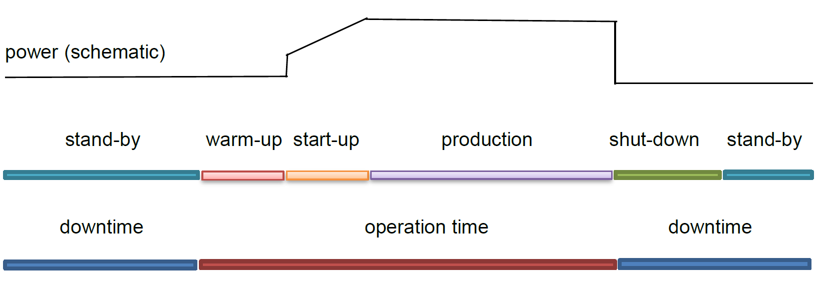
On the basis of characteristic parameters and curves of fcCHPs as well as explanations of the corresponding energetic correlations, we developed a general mathematical model which formally describes the relationship between primary energy demand as well as thermal and electrical energy supply. Therefore, the model distinguishes between different phases and explains the temporal dependencies between these phases. Within our model of a fcCHP we used the following physical parameters (constant values) of such power plants:
- •
A thermal efficiency factor and an electric efficiency factor (with respect to the primary energy source) such that .
- •
A maximal power output (thermal/electric) within the production phase resp. where because in general it applies that where is the power of the primary energy carrier.
- •
A minimal power output (thermal/electric) within the production phase resp. where .
- •
A minimal and maximal operation time resp. as well as a minimal off-time .
- •
a bounded, monotonically increasing function to determine the warm-up time depending on its recent off-time , i.e., .
- •
A constant electric power input during stand-by phases: .
- •
Some constant primary and electric power inputs during the warm-up phase: and . There, a cold-start requires additional input power: and .
- •
An additional constant electric power input during shut-down: during the short shut-down interval . This means that electric power input from the production phase to the stand-by phase has the power peak .
- •
A constant thermal and electric output power “peak” at the beginning of the start-up phase from zero to resp. to within a (short) constant time interval where applies.
- •
A constant power enhancement within a constant start-up phase to a final power value: It is assumed that the total duration of the start-up phase as well as the final power value are given such that applies. Thus, the constant power enhancement is . Consequently, the electric power enhancement results from .
- •
A maximal gradient for power modulation in the production phase: resp. .
The chosen MIP model of fcCHPs uses discrete time units. Therefore, the considered scheduling horizon is divided into equidistant time intervals of equal duration -- typically of 15 min22 2 A one-day scheduling horizon is subdivided into 96 time units., however, other time unit durations are possible, too. It is assumed that a fcCHP is either in operation or down within one time unit. Discretization of time is a common approach in mathematical modeling of dynamic processes. Further, it is compatible with the time units used in short-term energy markets. This means that a scheduling horizon is divided into time units / intervals of the same duration, namely .
The minimum and maximum operating durations (in time units) are therefore and and the minimum downtime is time units.
The decision whether a fcCHP is switched on or off (operation time vs. downtime) is always made for a complete time unit (i.e., for a time interval ). For this purpose, Boolean decision variables are introduced and applies if the fcCHP is on at time unit and if it is off at time unit , where indicates the on/off state at the beginning of the scheduling horizon which is known in advance. Furthermore, for the start variables are Boolean decision variables which determine whether the fcCHP starts in time unit (start of the operating phase) or not, i.e., and applies or not. There, for indicates any potentially interesting start event in the past which is known in advance. Similarly, the stop variables are Boolean decision variables which determine whether the fcCHP is switched off in time unit (begin of the down phase) or not, i.e., and applies or not.
In order to ensure that the start and stop variables are compatible with the on/off variables, the following conditions must be met (cf. [2]). There, the status of the fcCHP immediately before the start of the scheduling horizon, namely , is relevant:
| for . |
In order to further ensure that neither the minimum operating times nor downtimes are undercut, the following conditions must also be fulfilled:
| for . |
Example 1
Let a fcCHP with a minimal operation time time units be given. Further let and . Then for any admissible schedule must apply, i.e., the fcCHP must be operative (“on”) at time unit 1, otherwise its minimal operation time is undercut.
In order to limit the operating time, further auxiliary integer variables are required, such that the difference corresponds to the duration (in time units) from the last stop or start when starting or stopping at time unit assuming that a stop follows a start and vice versa. For this purpose let be the non-positive time unit at the last start or stop just before the beginning of the considered scheduling horizon. For any time unit the last start/stop time unit is kept if the on/off status of the fcCHP doesn’t change: If applies, then let . Otherwise, if there is change of the status the last start/stop time unit is updated: If applies, then let . Combining both cases results in:
| (3) |
Example 2
Let a fcCHP be given which runs from time unit -3 (already running at the beginning of the scheduling horizon) to time unit 13. Consequently , and apply. Thus, but apply due to the fact that and . Then the difference defines the recent operation time of the fcCHP in time units.
In general, Equation (3) cannot be processed directly by a MIP-Solver, because it contains products of Boolean terms and decision variables. Therefore any such product with and has to be replaced by a new auxiliary decision variable and the additional linear inequalities
The replacement is correct: On the one hand it follows from that applies and therefore . On the other hand if follows from that applies and therefore . In summary, applies.
Furthermore, Equation (3) contains the absolute amount of a difference. However, any equation can be modeled by means of a new auxiliary Boolean variable and some additional linear constraints
Consequently, either or applies depending on the value of . Since must not be negative, applies.
In order to ensure that the maximum operating time is not exceeded, the following must therefore apply:33 3 Here and in the following there are products of Boolean terms and decision variables, too.
These auxiliary variables are also useful to determine the duration of downtimes, which will be and thus the duration of warm-up times, which will be .44 4 Remember that the function maps downtimes to warm-up times, see above.
If the downtime is greater than a specified value , this is referred to as a cold start. Auxiliary Boolean variables are given, such that the value of in the warm-up phase indicates whether this occurred after a cold start, i.e., is implied:
for , a sufficiently large value and a corresponding value , e.g., known from a previous scheduling horizon. If the modeled fcCHP is starting at time unit then and apply. If this start event is a cold start, i.e., if applies, then applies, too. If follows that applies, otherwise there is a violation. If indicates that a downtime will require a cold-start and there is not any start event at time then is implied further indicating a cold-start, because applies, otherwise there is violation.
The determination of the warm-up times requires additional auxiliary integer variables , such that the value of corresponds to the last warm-up time. To do this, let be the warm-up time from the previous scheduling horizon. If applies, let . Otherwise, if applies, let . Combining both cases results in
Due to the fact that the argument of the function is variable, i.e., not known in advance, the computation of for a variable (assuming that the maximum downtime is shorter than the scheduling horizon) requires additional auxiliary Boolean variables . Then the condition
ensures that applies for . Consequently, it applies
where the supporting values are technical parameters of the fcCHP which are known in advance.55 5 applies due to the fact that is monotonically increasing, see above.
Furthermore, Boolean decision variables are introduced such that applies if and only if the modeled fcCHP warms up in time unit . In particular it applies that . Additionally, are Boolean decision variables that determine whether the fcCHP has completed the end of the warm-up phase in time unit (i.e., the start of the production phase) or not, i.e., and apply. In order to ensure that these “stop of warm-up” variables are compatible with the “warm-up” variables, the following conditions must be met, whereby the “warm-up” state of the fcCHP immediately before the start of the scheduling horizon – determined by – is relevant:
| for . |
A minimal duration of the warm-up phase has to be guaranteed. Therefore for each time unit and for each possible warm-up duration an auxiliary Boolean variable is defined such that if and only if a start occured no longer than time units before time unit :
Then the minimal warm-up time is satisfied, if
applies for and . This means that if is positive and the start is no longer than time units ago, i.e., , then the fcCHP is in the warm-up phase, i.e., must apply.66 6 N.B.: always applies, see above.
For an upper boundary of the warm-up time, additional auxiliary integer variables are necessary. Let be given such that represents the index of the last (i.e., most recent) start. Therefore let be the time unit of the latest start before the scheduling horizon. Now if then will apply, otherwise :
| (5) |
Then the maximal warm-up time is satisfied, if
| (6) |
This means that if the fcCHP warms up at time unit , then the latest start is no longer than the warm-up time ago.
At the end of the warm-up phase, the start-up phase begins, the duration of which is known in advance from the fcCHP characteristics. The same applies to the thermal and electrical power available in the start-up phase. In detail, there are time units with power jump, in general one time unit at with parts of the power jump and gradual starting (if and then time units in which the power increases constantly up to a given target value with . The end of the start-up phase is thus after further StartUp time units reached. This means that discrete power levels can be determined for primary energy and electricity consumption as well as for thermal and electric output power (abstract ). One type is sufficient, the others behave proportionally according to their efficiency factors:
Analogously to these power steps and due to the discretization there result electric power steps from during the shut-down phase (mostly one time unit because the duration of the shut-down phase is in general short):
where is the duration of the shut-down phase in time units.
The time units of the “jump” phases are characterized by Boolean decision variables where , if the fcCHP makes a performance jump in time unit and , if it is not the case in this time unit :
Boolean decision variables are introduced for the following production phase. will apply, if the fcCHP is productive in time unit , i.e., delivering thermal and electrical power and will apply, if it is not in the production phase in time unit , i.e., in particular, it applies that . In order to ensure that these “productive” variables are compatible with the corresponding start/stop variables, the following conditions must be met, whereby the status of the fcCHP directly before the start of the scheduling horizon – determined by – is relevant:
| for . |
Summarizing, the thermal power supply (output) of a fcCHP at time unit is characterized by the following equation:
where the values of the variable must lie within a specified performance band in the production phase, i.e., and the gradient of the value change is limited:77 7 How to model the absolute amount of a difference has already been explained.
The electrical power supply (output) results directly from the thermal power supply:
The electrical power demand (input) of a fcCHP depends on whether there is a cold-start or a warm-start:
There, the conjunction of two Boolean variables will be represented by an auxiliary Boolean variable satisfying for .
Analogously, the primary power demand (input) of a fcCHP over the production phases depends also on whether there is a cold-start or a warm-start:
In Figure 2, typical thermal and electric power profiles of a fcCHP are shown according to the presented MIP model. These profiles are matching the profiles measured by the fcCHP manufacturer giving some evidence that the energetic behavior of fcCHP is modeled adequately.

Assuming that the costs for primary energy at time unit , as well as the costs for switching on and for switching off a fcCHP, as well as the costs for the wear and tear per time unit during heating up , during cold start and during productive operation are known, then the costs for the operation of a fcCHP in time unit result directly:
This is only a simplified approach for the consideration of wear and tear costs of a fcCHP. For instance, aging effects are not taken into account. Although an aging approach can be converted into a linearly approximated model, initial run-time investigations result in very long computation times for cost optimization. However, the resulting operational plans hardly differ qualitatively from those with simplified models.
4 Implementing a MIP-Based Optimizing Tool
A software named “MIP Optimizer” is realized to transfer specifications of building energy systems into MIP models and then based on these models to determine cost-minimal operation schedules for the specified energy system components, so that predicted energy requirements for heating or cooling, domestic hot water and electricity over a given scheduling horizon are covered. In detail, the MIP Optimizer generates a MIP optimization problem from a formal description of the energy system components, i.e., the configuration of the energy system and from a formal description of the demand and the environmental and operational situation over the scheduling period. For this purpose, both formal descriptions determining the general configuration and the current situation are to be specified in XML files (cf. [13]) and must comply with a fixed XML schema (XSD) [14]. Energy demand profiles and other time series predicting the environmental situation (e.g., fluctuating primary energy prices or volatile PV power) shall be provided in files in Hierarchical Data Format (HDF5) [7, 5], referred to in the XML descriptions. Examples of the XML configuration and situation files are presented in Section 5.
Then, the MIP Optimizer uses the ColiopCoin Mathematical Programming Language (CMPL) [12] to generate and solve the optimization problem, since various MIP problem solvers can be used, such as the freely available Cbc [6] or the commercial CPLEX [10]. The operation schedules of the components of the building energy system are then extracted from the solution and stored in the form of time series in an HDF5 file, such that these data can be further used by a building management system to control the energy components.
The MIP Optimizer is implemented in Java and has a modular structure. Due to the modular modeling approach (cf. Section 3) and its object-oriented implementation, flexible extensions including further energy systems components are supported by design.
5 Evaluation on a Heat Pump Scenario
In order to prove the usefulness of our MIP-based optimization approach, generated operational schedules for building energy systems are considered. For this purpose, we considered a residential building, i.e., a single family detached house, according to the EnEV standard 2014 with usable area (Berlin site), an air-to-water heat pump with hot water storage tank for heat supply.
It was investigated, how an efficient operation can be planned with the help of the MIP Optimizer as cost- and energy-efficient as possible by predicting the Coefficients of Performance (COP) of the heat pump dependent on the outside temperature and the residential heat demand. The building energy system consists of a heat pump and a heat storage. The heat demand and COP of the heat pump changing with the outside temperature were determined and provided by our project partners at Berlin University of the Arts, Institute for Architecture and Urban Planning, Department of Building Physics and Building Technology. These partners used weather forecasts and Modelica to model and simulate the thermal behavior of the selected building.
In the subsequent operational scheduling, partial models of a heat pump with a constant electrical power consumption of 1.8 kW in operation (cf. the XML element <HeatPump> below) and of a heat storage tank with a charging capacity of 20.82 kWh (cf. the XML element <HeatBuffer> below) were combined at an ambient temperature of to form an overall model of the energy system. Electricity prices, the heat demand profiles determined by simulation and time-dependent COP as well as the system status data (e.g., state of charge of the heat storage tank) were added. The description of the building energy system was specified in XML as a configuration with characteristic physical parameters, which were further processed by the MIP Optimizer:
Actual and predicted data were also transferred to the MIP Optimizer with the help of a situation description, also in XML, whereby the time series for heat demand, COP, electricity prices etc. were to be found in separate HDF5 files to which references are made:
In detail, usage profiles are stored in HDF5 files (with file extension “.h5”), which are referenced in the respective XML elements (e.g., <ElectricPowerUsage>). The name of the file containing the operation schedules must be entered as the value of the attribute fileNameHDF5 in the XML root element <BuildingSituation>. After processing the models the optimized schedule of the heat pump is stored in this file.
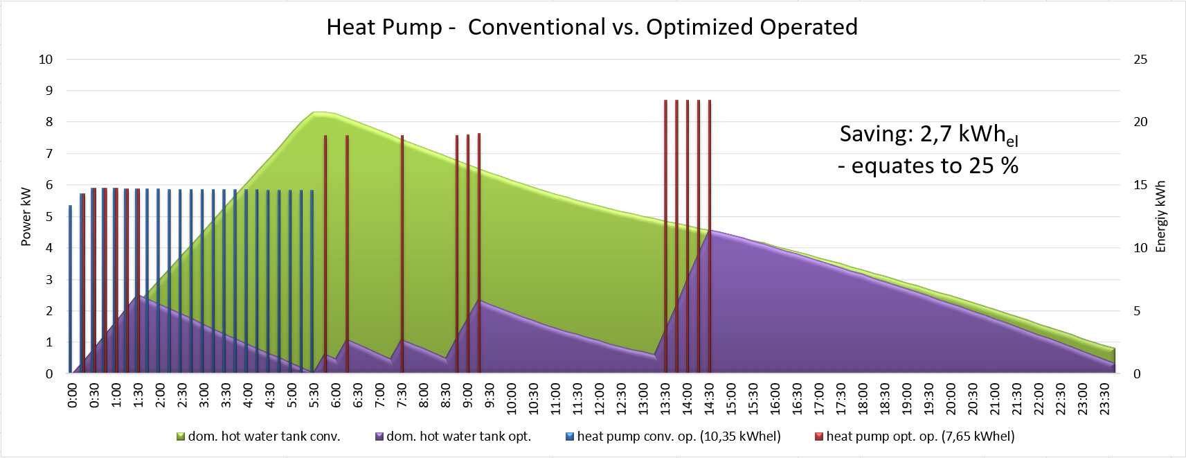
The resulting cost-minimized schedule of the operation of the building energy system (cf. Figure 3) shows that, in contrast to charging the thermal storage tank (TST) during the night hours (blue), an extensive operation of the heat pump at low outside temperatures and low COP can be avoided, if the heat demand and COP is known in advance and the heat pump is operated accordingly (red). Covering the currently predicted heat demand only enables a saving of 25 % electric energy, provided that the forecasts correspond to reality. Due to the general uncertainty of forecasts for energy supply and demand it is strongly recommended for practical applications to use some energy reservoirs, e.g., TSTs or batteries, and parts of their charging/discharging capacities as buffers to balance deviations.
6 Conclusion and Future Work
In this paper a MIP-based approach is presented to model and optimize the operation of building energy systems. In detail the modeling of the energetic behavior of fcCHPs is presented and it is shown how sub-models of different energy component can be combined reflecting their integration into building energy systems. By example it is shown that the approach can be applied successfully. However, a comprehensive analysis on the accuracy and adequacy of the MIP models and the impact of imperfect forecasts for energy demand/production and energy prices has the be performed in the future, maybe in a follow-up research and development project.
References
- [1] John E. Beasley. OR Notes – Separable programming. http://people.brunel.ac.uk/%7Emastjjb/jeb/or/sep.html.
- [2] M. G. C. Bosman, V. Bakker, A. Molderink, J. L. Hurink, and G. J. M. Smit. Planning the production of a fleet of domestic combined heat and power generators. European Journal of Operational Research, 216(1):140–151, January 2012.
- [3] Mohammad Chehreghani Bozchalui and Ratnesh Sharma. Optimal Operation of Commercial Building Microgrids Using Multi-Objective Optimization to Achieve Emissions and Efficiency Targets. In Power and Energy Society General Meeting, 2012 IEEE, pages 1–8, 2012.
- [4] Faeze Brahman, Masoud Honarmand, and Shahram Jadid. Optimal Electrical and Thermal Energy Management of a Residential Energy Hub, Integrating Demand Response and Energy Storage System. Energy and Buildings, 90:65–75, 2015.
- [5] Mike Folk, Gerd Heber, Quincey Koziol, Elena Pourmal, and Dana Robinson. An overview of the HDF5 technology suite and its applications. In Proceedings of the EDBT/ICDT 2011 Workshop on Array Databases - AD ’11, pages 36–47, Uppsala, Sweden, 2011. ACM Press.
- [6] John Forrest. CBC User Guide. https://www.coin-or.org/Cbc/cbcuserguide.html.
- [7] The HDF Group. HDF Home. https://www.hdfgroup.org/.
- [8] Wei Gu, Yiyuan Tang, Shuyong Peng, Delin Wang, Wanxing Sheng, and Keyan Liu. Optimal configuration and analysis of combined cooling, heating, and power microgrid with thermal storage tank under uncertainty. Journal of Renewable and Sustainable Energy, 7(1):013104, January 2015.
- [9] Wei Gu, Zhi Wu, Rui Bo, Wei Liu, Gan Zhou, Wu Chen, and Zaijun Wu. Modeling, Planning and Optimal Energy Management of Combined Cooling, Heating and Power Microgrid: A Review. Electrical Power and Energy Systems, 54:26–37, 2014.
- [10] IBM. ILOG CPLEX Optimization Studio - Survey. https://www.ibm.com/products/ilog-cplex-optimization-studio, January 2019.
- [11] Matti Järvisalo, Emilia Oikarinen, Tomi Janhunen, and Ilkka Niemelä. A Module-Based Framework for Multi-language Constraint Modeling. In Esra Erdem, Fangzhen Lin, and Torsten Schaub, editors, Logic Programming and Nonmonotonic Reasoning, Lecture Notes in Computer Science, pages 155–168. Springer Berlin Heidelberg, 2009.
- [12] Mike Steglich and Thomas Schleiff. CMPL: Coliop Mathematical Programming Language - Version 1.12 - March 2018, 2018.
- [13] W3C. Extensible Markup Language (XML). https://www.w3.org/XML/.
- [14] W3C. XML Schema. https://www.w3.org/XML/Schema.