Rate-Memory Trade-off for Multi-access Coded Caching with Uncoded Placement
Abstract
We study a multi-access variant of the popular coded caching framework, which consists of a central server with a catalog of files, caches with limited memory , and users such that each user has access to consecutive caches with a cyclic wrap-around and requests one file from the central server’s catalog. The server assists in file delivery by transmitting a message of size over a shared error-free link and the goal is to characterize the optimal rate-memory trade-off. This setup was studied previously by Hachem et al., where an achievable rate and an information-theoretic lower bound were derived. However, the multiplicative gap between them was shown to scale linearly with the access degree and thus order-optimality could not be established.
A series of recent works have used a natural mapping of the coded caching problem to the well-known index coding problem to derive tighter characterizations of the optimal rate-memory trade-off under the additional assumption that the caches store uncoded content. We follow a similar strategy for the multi-access framework and provide new bounds for the optimal rate-memory trade-off over all uncoded placement policies. In particular, we derive a new achievable rate for any and a new lower bound, which works for any uncoded placement policy and . We then establish that the (multiplicative) gap between the new achievable rate and the lower bound is at most independent of all parameters, thus establishing an order-optimal characterization of for any . This is a significant improvement over the previously known gap result, albeit under the restriction of uncoded placement policies. Finally, we also characterize exactly for a few special cases.
I Introduction
The rapid increase in the usage of smart devices has lead to an unprecedented growth in internet traffic. A recent study [3] shows that data traffic from Video on Demand (VoD) services will increase exponentially in the forthcoming years. One way to meet this rise in demand is by prefetching and caching some of the data locally. Motivated by this, we study a cache-aided content delivery network (CCDN), as shown in Figure 1.
In the last few years, there has been a lot of interest in characterizing the fundamental performance limits of the cache-aided content delivery network (CCDN), see for example [4, 5]. A CCDN consists of a central server with a catalog of files, a collection of users, and several caches with limited storage capabilities. The caches can pre-fetch and store some of the content from the server, such that when users request files from the central server, the caches help the central server in serving the user requests. The main challenges in a CCDN are designing the (i) placement policy, which decides what to store in the caches, (ii) delivery policy, which decides how to serve the user requests, with the goal of minimizing the server’s transmission rate.
In particular, the seminal work of [6, 7] studied the fundamental limits of server’s transmission rate of a particular CCDN setup (Ali-Niesen setup) which is as follows: there is a central server with files of unit size and users, each one associated with a distinct cache of size units. Each user requests a file from the central server and based on the request profile as well as the content stored in the caches, the server broadcasts messages on a shared error-free link to the users. The goal is to minimize the server’s transmission rate while ensuring that each user can recover its’ requested file. [6] proposed a (uncoded) placement and (coded) delivery policy for this setup and analyzed the achievable server transmission rate of the scheme as a function of parameters of the system (). Moreover, [6] also showed that the rate achieved by the policy is within a constant multiplicative factor () of the information-theoretic optimal rate by comparing it to a lower bound, which assumes no restrictions on either the placement or the delivery policy used. Following the initial papers, there have been significant improvements in terms of both the achievable rates [8, 9, 10, 11, 12] as well as the lower bound arguments [13, 14, 15, 16] which can be used to tighten the gap significantly. In fact, under the natural restriction of an uncoded placement phase where caches are not allowed to store coded content, the rate proposed in [6] is shown to be exactly optimal in [17, 18]. This is done by mapping the CCDN setup to the well-studied index coding problem (ICP) [19, 20] (described in Section IV) and using the bounds available in the literature for the ICP.
Several variants of the above setup have been studied in the literature, see for example [21] for an extensive survey. In particular, [22] studied a generalization of the Ali-Niesen setup where instead of each user accessing a single (distinct) cache, every user has access to multiple () consecutive caches (with a cyclic wrap-around), as shown in Figure 1. This was motivated by the upcoming heterogeneous cellular architecture which will consist of dense deployment of wireless access points (APs) with small coverage and relatively large data rates, in addition to sparse cellular base-stations (BSs) with large coverage and smaller data rates. Placing caches at local APs can help reduce the BS transmission rate, with each user capable of accessing the content stored at multiple nearby APs in addition to receiving the BS broadcast. For this multi-access CCDN, [22] proposed a coloring based placement and delivery policy and analyzed its’ achievable rate . By comparing this rate to the information-theoretic optimal rate which puts no restrictions on either the placement or the delivery policy used, [22, Theorem 4] showed that , where is some constant, independent of all system parameters. Thus, the gap between the achievable rate and the information-theoretic lower bound increases linearly with , the number of caches each user has access to, and the obvious challenge is to improve the achievable rate and/or lower bound to establish the exact optimal rate-memory trade-off or at least up to a constant factor for any .

In this paper, we study the same multi-access setup and make the following technical contributions:
- •
derive a new achievable rate for the general multi-access CCDN with , based on a scheme using uncoded placement; can be order-wise better than the best previously known rate [22],
- •
derive a general lower bound on the optimal rate for any multi-access CCDN with , under the restriction of uncoded placement,
- •
establish order-optimal (up to a multiplicative factor of ) uncoded placement rate-memory trade-off for any multi-access CCDN with ,
- •
establish exact optimal uncoded placement rate-memory trade-off for a few special cases, for example ; ; with even.
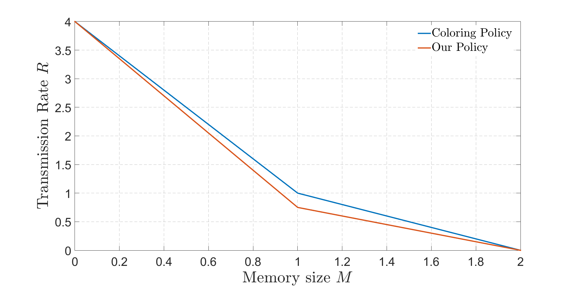
As mentioned before, [22] derived an achievable rate and an information-theoretic lower bound which differ by a multiplicative gap scaling linearly with . Using an improved achievable rate as well as a better lower bound under the restriction of uncoded placement, we are able to establish the uncoded placement rate-memory trade-off for any multi-access CCDN with up to a constant factor, independent of . To illustrate the gains of our policy over the coloring based policy in [22], we plot
- 1.
the rate-memory trade-off for the ()-CCDN in Figure 3. For this system, our policy performs better than the coloring based policy in all the memory regimes. Moreover, as we show in Appendix I, our policy in fact achieves the optimal rate-memory trade-off.
- 2.
the transmission rate at the memory point as a function of the number of users/caches for an ()-CCDN in Figure 3. As the plot shows, the additive gap between the performance of the two schemes increases linearly with .

Our results are based on mapping our multi-access CCDN setup to appropriate index coding problems [19] and finding bounds on their solutions, which might be of interest in their own right. The index coding problems that result from our mapping are similar in spirit to those studied in [23, 24, 25]. Similar index coding-based approaches have been used recently to study other variants of the original coded caching problem and for designing better achievability schemes as well as prove converses under the restriction of uncoded placement [26, 27, 28, 29, 30, 31, 32, 33, 34].
The rest of the paper is organized as follows. Section II briefly describes the problem setting, while Sections III and IV describe some useful notations and preliminaries. Section V and Section VI describe our policy and the main results. The summary of our work and future goals are given in Section VII and the proofs of our main results are given in Section VIII.
II Problem Setting
We consider a cache-aided content delivery network (CCDN) which consists of a central server, users, and caches as shown in Figure 1. We assume,
- •
the central server contains files , each of size unit (= bits22 2 We will assume the file size to be large),
- •
each user has access to consecutive caches with a cyclic wrap-around33 3 For symmetry, we assume that Caches 1 and are adjacent. as shown in Figure 1,
- •
cache sizes are uniform and are units each,
- •
each user requests one file which has to be served by a central server’s message, and the content in the caches it has access to, and
- •
the communication channel between the central server and the users is an error-free shared (broadcast) channel.
We will refer to the above system as the ()CCDN.
The system runs in two phases: a placement phase and a delivery phase.
II-1 Placement Phase
In the placement phase, we fill the caches with the content related to the files. Like [18, 17], we restrict to an uncoded placement phase. We are allowed to split the files into parts and store the file parts, but coding across the file parts is not allowed while storing in the caches. The placement phase occurs before users reveal their requests and hence is independent of user requests.
After the placement phase, each user (User j) requests one file (File ) from the central server, chosen arbitrarily from amongst the files. We call () as the request profile.
II-2 Delivery Phase
In the delivery phase, depending on the request profile () and content stored in the caches, the central server broadcasts a message of size units such that each user can recover their requested file using the server transmission and the content in the caches it has access to. We refer to the message size as the server transmission rate.
A rate-memory pair () is said to be achievable for request profile if there exists a placement and delivery scheme with server transmission rate for cache size , such that every user (User ) can recover its requested file (File ). A rate-memory pair () is said to be achievable if this pair is achievable for any possible arbitrary request profile. For a given cache size , we define optimal rate-memory trade-off as the smallest rate for which the rate-memory pair () is achievable. Our goal is to characterize under the restriction of uncoded placement and come up with a placement and delivery policy that achieves .
As mentioned in Section I, [22] studied this setup with multi-cache access () and proposed a coloring-based achievability scheme which builds on the coded delivery ideas presented in [6, 7] for single cache access (). For the general setup, the server transmission rate for this scheme is given by
For general , the lower convex envelope of these points is achievable via memory-sharing. Incidentally, the proposed scheme used uncoded placement and coding is used only in the server broadcast message.
In this paper, we derive a new achievable rate for the general multi-access CCDN with , based on a scheme using uncoded placement, which can be order-wise better than the best previously known rate [22]. Our new achievable rate is exactly optimal for a few cases and order wise optimal for any .
III Notations
- •
.
- •
- •
- •
denotes the cardinality of a set or size of a file/subfile.
- •
denotes parts of File exclusively available to users with index in set .
- •
denotes the power set of set .
IV Preliminaries
We map our setup to the well-studied index coding problem (ICP) [19] and use some of the ideas developed for this problem to characterize the optimal rate-memory trade-off for our setup. Similar to our setup, ICP has a server with a catalog of say files. There are nodes, such that Node requests File and has access to a subset of the remaining files . is called the side information of Node . Depending on the side information profile, the server broadcasts a message so that each node can recover its requested file using the broadcast message and the side information available. The goal is to characterize the minimum broadcast rate for any given instance of the ICP.
Even though the ICP and our problem setting look similar ({server, node requests, side information} {central server, user requests, accessible caches content}), the differences between the ICP and our problem setup are
- 1.
in an ICP problem, the side information is already given whereas, in our setup, we have the choice of what to store in caches.
- 2.
in an ICP problem, the node requests are fixed whereas, in our setup, the user requests are arbitrary.
Once the cache contents are fixed and user requests are revealed, then the problem of minimizing the central server’s broadcast rate in our setup is equivalent to that for a corresponding ICP.
In an ICP, Node is said to be interfering with Node , if Node does not have File as side information. Let denote the closed anti-outneighborhood of a Node which is defined as the set containing Node itself and all its interfering nodes. A coloring scheme for an ICP assigns a color to each node and is said to be proper if no node shares its color with any of its interfering nodes. Let be a proper coloring scheme with (any positive integer) colors and denote the number of colors in the closed anti-outneighborhood of the Node . Then, the local chromatic number of an ICP () is defined as
In words, the local chromatic number of an ICP is defined as the maximum number of different colors that appear in the closed anti-outneighborhood of any node, minimized over all proper colorings.
We use the following result to upper bound the broadcast rate of an ICP, which follows from [35, Theorem 1].
Lemma 1
Given an node ICP, the minimum broadcast rate of the ICP is upper bounded by its local chromatic number .
We can represent an node ICP by an equivalent vertex directed side information graph , where each vertex corresponds to a unique node, and there exists an edge from Vertex to Vertex if Node has File (Node ’s requested file).
There are several available lower bounds for the ICP. In particular, we use Lemma 2 to derive a lower bound on the server transmission rate for our multi-access CCDN and it follows from [36, Corollary 1].
Lemma 2
Consider an node ICP with side information graph . Let be the file requested by Node and be the minimum broadcast rate. Then, for any subset such that the subgraph of induced by the vertices in does not contain a directed cycle, we have
V Our Policy
In this section, we describe our policy with an example. Our policy can have a lower server transmission rate than the coloring-based policy proposed in [22]. Our placement and delivery policies, both are different to the coloring-based policy. Our delivery policy is based on a solution to an appropriately defined ICP.
Consider a general -CCDN setup. We first describe our achievable scheme for corner points, i.e., for memory points , where .
V-A
If , then , i.e., no file parts are stored in the cache. The worst-case request pattern is all users requesting different files. Hence,
V-B
First, we define the term as follows:
| (1) |
In words, is the collection of subsets of which satisfy (i) , and (ii) if , every two distinct elements of satisfy and .
V-B1 Placement policy
Divide each file into parts, with one subfile corresponding to each subset . Store the subfile corresponding to set in all the caches whose index belongs to .
The above policy creates overlaps in the cache contents to increase coded-multicasting opportunities while ensuring that there are no redundant copies. For example, a user should not have two copies of the same subfile amongst its accessible caches.
V-B2 Delivery policy
After users have revealed their requests, form an instance of the ICP with the file parts which are unavailable locally. The server transmits messages according to the solution of the ICP.
V-C
We first create a list (of size elements) by repeating the sequence times, i.e., . Then we fill the caches according to the list sequentially. Note that the total memory required to fit the list is units, which is equal to our total cache memory. Hence, the memory constraint is satisfied. This storage policy makes sure that each user has access to all files in the central server’s catalog. Hence, the worst-case transmission rate is 0 units.
Example: For () CCDN, at , the list is and Cache 1 is filled with files 1 and 2, Cache 2 is filled with files 3 and 1, Cache 3 is filled with files 2 and 3. Observe that with this storage policy, each user has access to all the files. Hence, the worst-case transmission rate is 0 units. For the remaining points , our achievable rate is derived by memory sharing.
Now, we illustrate our policy with an example.
Example: () CCDN
Consider an example with files, users / caches and each user connected to caches, as shown in Figure 4.
We discuss the achievability for memory points . At the remaining points, achievable rate is obtained by memory sharing.

V-A units
When M = 0, no file parts are stored in the cache. The worst case request pattern is all users requesting different files. Hence,
V-B unit
V-B1 Placement policy
At , . Hence, . Split each file into parts and store the part of each file in Cache 1, the part of each file in Cache 2, and so on as shown in Figure 4. Observe that the memory constraint () is satisfied. Since the cache is connected to User 4 and User 1, we subscript the stored content in Cache 1 with , and repeat the same procedure for the other caches as well, i.e.,
- •
Cache 1 stores , , and ,
- •
Cache 2 stores , , and ,
- •
Cache 3 stores , , and ,
- •
Cache 4 stores , , and .
V-B2 Delivery policy
Let the user request profile be . In terms of subfiles,
- •
User 1 needs , , and ,
- •
Uset 2 needs , , and ,
- •
User 3 needs , , and ,
- •
User 4 needs , , and .
Note that the red color (bold font) subfiles are already available at the corresponding users, only the black color (normal font) subfiles are needed for them. Each user requires 2 subfiles and thus a total 8 subfiles are involved in the server transmission. We can map the problem here to an instance of the index coding problem described in Section IV, with nodes, each one requesting a distinct subfile. The side information at the node representing (and requesting) some Subfile are the subfiles available to the user which is requesting Subfile . For example, the side information of the node representing Subfile are the subfiles available to User 1, i.e., , , , and . We can solve this index coding problem to get the achievable transmission rate for our proposed scheme. Note that the number of messages transmitted by the central server in the CCDN is equal to the number of messages transmitted in the ICP, and the size of each message is equal to the size of a subfile.
To understand the structural properties of the above ICP, we form a table (see Table 2), such that the row and column contains Node , i.e., the subfile requested by User and available at users . We refer to this entry as the Node where, . Note that the entries in the Row are the subfiles needed for User . We will use the notation to represent all the other nodes in Row excluding Node . For our example represents Node and represents Node .
| 1 | 3 |
|---|---|
| 2 | 4 |
| 3 | 1 |
| 4 | 2 |
Recall from Section IV that the minimum broadcast rate of an ICP is upper bounded by its local chromatic number. A coloring scheme for an ICP is said to be proper if no node shares its color with any of its interfering nodes. Observe that for Node in Table 2, among the other nodes, only nodes , , and do not contain in the set which is represented by their subscripted rectangular brackets, and are thus interfering nodes. We take colors and for each assign Color to nodes and . The coloring scheme is shown in Table 2. The interfering nodes for nodes in the Row are present in rows , , but we repeat the color of Node () for its non-interfering Node () and the color of Node () for its non-interfering Node (). So, this coloring scheme ensures that none of the nodes share its color with any of its interfering nodes. Hence, this is a proper coloring scheme.
The local chromatic number of an ICP is defined as the maximum number of different colors that appear in the closed anti-outneighborhood of any node, minimized over all proper colorings. Observe that for Node (), 3 colors appear in the closed anti-outneighborhood, one color for Node (), one color for Node (), one common color for nodes () and (). Hence, an upper bound on the local chromatic number of the ICP is 3. Therefore, the central server transmits at most 3 messages to serve all the users.
In this case, it is possible to get an explicit characterization of the optimal server transmission scheme and it is given by:
It can be verified that using the above server transmissions and the accessible cache contents, each user can recover its requested file. Since each message is of size units, the total server transmission size is given by
V-C units
Store files , in Cache 1, Cache 3 and , in Cache 2, Cache 4. Since each user has access to all files, the worst case transmission rate is
The transmission rate at intermediate values is given by memory-sharing and thus the achievable rate-memory trade-off of our scheme is given by
| (2) |
On the other hand, the achievable rate for the coloring-based scheme proposed in [22] is given by
| (3) |
Figure 3 shows the comparison between the performance of the two schemes and demonstrates the improvement in rate using our modified placement scheme and an associated index coding-based delivery scheme.
VI Main Results
Now we evaluate the performance of our policy in this section and characterize the optimal rate-memory trade-off for multi-access coded caching system. As mentioned in Section IV, most of our results are based on ICP bounds. The proofs of our results are relegated to Section VIII.
VI-A New achievable rate for general (, , )CCDN
First, we provide a new upper bound on for the general (, , )CCDN using our (uncoded) placement and delivery policy.
Theorem 1
Consider the general () CCDN with . Let be the cache size, and be the optimal rate-memory trade-off under the restriction of uncoded placement. Then for , ,
is achievable using an uncoded placement scheme. For general , the lower convex envelope of these points is achievable.
As mentioned earlier, [22] gave an upper bound44 4 The proposed scheme had an uncoded placement phase for the case when divides . on , which is given by . Our achievable rate in Theorem 1 can sometimes be significantly better than , see example below.
Example: For ()CCDN, is a constant whereas grows unbounded as the number of users in the system increases.
Next, we specialize the result in Theorem 1 to the case of , which is the regime for our remaining results.
Corollary 2
Consider the CCDN with . Let be the cache size, be the optimal rate-memory trade-off under the restriction of uncoded placement, then
| (4) |
Proof:
Proof: From Theorem 1, the achievable rate at memory points , , and is , , and respectively. The convex envelope of these points is . Hence . ∎
VI-B Order optimality for
As mentioned before, the gap between the achievable rate and the information-theoretic lower bound derived in [22] scales with , i.e., , where is the information-theoretically optimal rate-memory trade-off and is some constant. While the characterization (exact or order-optimal) of for a general ()CCDN remains open, our following results establish the order-optimal (up to a factor of ) uncoded placement rate-memory trade-off for any CCDN with . For this, we provide an improved lower bound on the server transmission rate for any valid (uncoded) placement and delivery scheme in Theorem 3 and use the upper bound stated in Corollary 2. We derive the lower bound by mapping our setup to an appropriate ICP and using converse arguments for the ICP to derive lower bounds on the server transmission rate for our setup. Let be defined as follows:
| (5) |
Theorem 3
Consider the -CCDN with . Let be the cache size, be the optimal rate-memory trade-off under the restriction of uncoded placement, and be as defined in (5). Then we have
The following corollary compares the upper and lower bounds on from Corollary 2 and Theorem 3 respectively and gives an approximate characterization of the optimal rate-memory trade-off .
Corollary 4
Consider the -CCDN with . Let be the cache size, be the optimal rate-memory trade-off under the restriction of uncoded placement and be as defined in (4). Then we have
We are able to give an approximate characterization of the optimal rate-memory trade-off for , because of improvement in both the upper and lower bounds.
VI-C Exact optimality for some special cases
While Corollary 4 provides an approximate characterization of , for any , we now present some special cases where we are able to derive it exactly.
Theorem 5
Consider the -CCDN with . Let be the cache size, be the optimal rate-memory trade-off under the restriction of uncoded placement, and be as defined in (5). Then for any cache size , we have for the following scenarios:
- 1.
,
- 2.
,
- 3.
= , is even,
- 4.
for some positive integer .
The above result is proven by deriving improved achievability bounds for the mentioned cases and showing that the rate-memory pair () is feasible for all . This combined with Theorem 3 then gives us the above result. Note that for = , we are able to characterize exactly when is even. For the case of = with odd, we are able to show that the rate-memory pair () is achievable, where is defined as follows:
Comparing to the lower bound from Theorem 3, we can show that the additive gap is at most , which decreases to zero as the number of users in the system becomes large.
VII Discussions
In summary, we derived new bounds for the ()CCDN and established the order-optimal uncoded placement rate-memory trade-off for the case of . We also established the exact uncoded placement rate-memory trade-off for a few cases. Note that while our achievable rate works for any , our lower bound is specifically tailored towards the case of . Generalizing this bound to the case of and using it to extend the order-optimality result to this regime are natural directions for future research.
While our ultimate goal is to characterize the exact rate-memory trade-off for the general -CCDN problem, there are several challenges involved. While our proposed scheme works for the general setup, characterizing its rate-memory trade-off can be very difficult in general. This is because our achievability scheme is based on the solution of the corresponding ICP and that in general is an NP-hard [19] problem. It can also be quite difficult to get closed-form expressions for the known upper bounds. To get tighter upper bounds for the achievable rate of our proposed strategy is indeed a part of our future work.
Our lower bound is specifically tailored towards the case of . Generalizing this bound to the case of is also more challenging for the general setup. A critical step in proving the index coding-based lower bound (illustrated in Section VIII-A) was to generate several inequalities by considering different request patterns and different user orders , and then combining them. For the case, [18, 17] considered all possible permutations to get a tight lower bound. However, for the multi cache-access case with , not all user permutations are equivalent since some of the cache-access subsets are not feasible.
For example, consider the -CCDN. Recall the lower bound argument discussed in Section VIII-A. For any request profile , if we use the user permutation , we will get the inequality , which contains one fewer term than the inequality we get for the user permutation , given by .
For , rotations (instead of permutations) for the user order are all equivalent and suffice to get a tight lower bound. Unfortunately, they do not suffice in the general case and hence, we need more sophisticated analysis to devise tight lower bounds for the general (, , )-CCDN setup. This is also part of our future work.
VIII Proofs
Here, we provide the proofs for all the results. The proofs are given in the following order: Theorem 3, Theorem 5, Theorem 1, and Corollary 4.
VIII-A Proof of Theorem 3
Proof:
In this section, we derive a lower bound on the server transmission rate for the general (, , )CCDN. We provide detailed calculations for the (, , )CCDN in Appendix I. Instead of including all the details for the general case here, which would have been very cumbersome, we refer to calculations in the appendix, at appropriate junctures through the proof in this section.
The server has files . Any uncoded placement policy divides each file into disjoint parts (subfiles), denoted by , where denotes the part of file which is available (via the caches) exclusively to the users in , and .
Let denote the total size of the file parts (in units) which are are each stored on caches and are available to users. Hence,
| (6) | |||
| (7) |
In our setup can be non-zero for only some of the possible pairs . After removing the combinations of and which are not possible, (6), (7) become
| (8) | |||
| (9) |
Following along similar lines as the converse for the (, , )-CCDN case given in Appendix I, we calculate a lower bound for a particular user rotation and request pattern first and then sum it over all possible user rotations and request patterns. Then, we get
Hence,
VIII-B Proof of Theorem 5
Proof:
VIII-B1 Placement Policy for any at
We have . From the definition of in (1), . We split each file into equal parts and store the part of each file in Cache . Observe that this storage policy satisfies the memory constraint units. Since Cache is connected to User , User ,…, User , we subscript the stored content in Cache with the set , i.e., Cache stores . Recall that User has access to caches , , …, . Hence, for all , , are available to User .
Example: Consider a ()CCDN. For all ,
- •
, and are available to User 1,
- •
, and are available to User 2,
- •
, and are available to User 3,
- •
, and are available to User 4,
- •
, and are available to User 5.
VIII-B2 Delivery Policy at
Now, we discuss the delivery phase. Let the user request profile be , i.e., User requests File . User needs only those File ’s subfiles which are not available to him. Explicitly, User needs only subfiles , , …, which are stored in User ’s non accessible caches , ,…, respectively.
Example: For a ()CCDN,
- •
User 1 needs and ,
- •
User 2 needs and ,
- •
User 3 needs and ,
- •
User 4 needs and ,
- •
User 5 needs and .
Each user needs subfiles and thus a total of subfiles are involved in the server transmission. We can map the problem here to an instance of the ICP described in Section IV, with nodes, each one requesting a distinct subfile. The side information at the node representing (and requesting) some Subfile are the subfiles available to the user which is requesting Subfile .
Recall from Lemma 1 in Section IV, the minimum broadcast rate of an ICP is upper bounded by its local chromatic number. For the cases mentioned in Theorem 5, we show that an upper bound on the local chromatic number of the corresponding ICP’s is , the details can be found in Appendix II. Since the server transmits at most messages, each of size units, the broadcast rate at is upper bounded by units.
Hence, for all the cases in Theorem 5, the transmission rates , and are achievable at memory points , and respectively. The transmission rates at the intermediate values are derived using memory-sharing arguments. It can be verified that the achievable rate expression matches the lower bound derived in Theorem 3 at all values of the memory . This concludes the proof of the theorem. ∎
VIII-C Proof of Theorem 1
Proof:
We first discuss the case. The proof follows along the same lines as Theorem 5. The placement scheme is identical and in the delivery phase, the key distinction is in the coloring scheme used for the corresponding ICPs.
VIII-C1 CCDN
For our achievability scheme, we consider 3 corner points . As mentioned in Section V the rates and are achievable at memory points and respectively. Now, we discuss the memory point .
We use the same placement scheme as given in the proof of Theorem 5, Section VIII-B and following the same arguments before, we get the ICP for as shown in Table 4. In the table,
- 1.
Row of the table represents User ’s needed subfiles,
- 2.
Node () is .
Observe that the subscripts of the elements in a column are sliding windows of length .
| … | |||
| … | |||
| ⋮ | ⋮ | … | ⋮ |
| … | |||
| ⋮ | ⋮ | … | ⋮ |
| … |
| 1 | 10 | 19 | 28 |
|---|---|---|---|
| 2 | 11 | 20 | 29 |
| 3 | 12 | 21 | 30 |
| 4 | 13 | 22 | 31 |
| 5 | 14 | 23 | 32 |
| 6 | 15 | 24 | 33 |
| 7 | 16 | 25 | 34 |
| 8 | 17 | 26 | 35 |
| 9 | 18 | 27 | 36 |
Recall from Section IV that a coloring scheme for an ICP is said to be proper if no node shares its color with any of its interfering nodes. For our ICP, we take colors and assign a unique color to each node. Explicitly, let the colors be . For Node assign Color . This is a proper coloring scheme. The coloring scheme for CCDN is shown in Table 4.
Consider any Node (). It can be verified that in each column, the index appears exactly times as subscript. Hence, every node has non-interfering nodes in every column. Therefore the closed anti-outneighborhood of any node contains nodes. For each node, we assign a different color. Hence, the local chromatic number of the ICP is . Therefore from Lemma 1, we broadcast messages. Since each sub-file is of size units, units units.
VIII-C2 CCDN
For our achievability scheme, we consider the corner points , . As mentioned in Section V the rates and are achievable at memory points and respectively. Now, we discuss the remaining memory points. Let , where .
Recall from Section V that in our policy, we divide each file into parts, with one subfile corresponding to each subset and store the subfile corresponding to set in all the caches whose index belongs to .
Let the user request profile be , i.e., User requests File . Some of the subfiles of File are already stored in User ’s accessible caches. Hence, User needs only those subfiles of File which are not stored in its accessible caches. It can be verified that the the number of subfiles needed for each user is . Like case, we map the problem here to an instance of the ICP described in Section IV, with nodes, each one corresponding to a distinct subfile. Now, we form a table with the following properties:
- 1.
Row of the table represents User ’s needed subfiles,
- 2.
If Node () is , then Node () is
.
The number of columns in the table is equal to the number of File ’s subfiles needed for User , which is equal to .
For this ICP, we take colors and assign one color for one node. Explicitly, let the colors be . For Node assign Color .
The subscript of a node contains elements. Consider any Node (). It can be verified that in each column, the index appears exactly times as subscript. Hence, every node has non-interfering nodes in every column. Therefore the closed anti-outneighborhood of any node contains nodes. For each node, we assign a different color. Hence, the local chromatic number of the ICP is bounded by . Therefore from Lemma 1, we broadcast messages. Since each sub-file is of size units, units. ∎
VIII-D Proof of Corollary 4
References
- [1] K. S. Reddy and N. Karamchandani, “On the exact rate-memory trade-off for multi-access coded caching with uncoded placement,” in IEEE International Conference on Signal Processing and Communications (SPCOM), 2018, pp. 1–5.
- [2] ——, “Rate-memory trade-off for multi-access coded caching with uncoded placement,” in IEEE International Symposium on Information Theory (ISIT), 2019, pp. 1232–1236.
- [3] Cisco Whitepaper: https://www.cisco.com/c/en/us/soluti ons/collateral/service-provide r/visual-networking-index-vni/white-paper-c11-741490.html.
- [4] Caching for Communication Systems and Networks, vol. 36, no. 6, 2018.
- [5] Caching for Communication Systems and Networks, vol. 36, no. 8, 2018.
- [6] M. A. Maddah-Ali and U. Niesen, “Fundamental limits of caching,” IEEE Transactions on Information Theory, vol. 60, no. 5, pp. 2856–2867, 2014.
- [7] ——, “Decentralized coded caching attains order-optimal memory-rate tradeoff,” IEEE/ACM Transactions on Networking, vol. 23, no. 4, pp. 1029–1040, Aug 2015.
- [8] M. M. Amiri and D. Gündüz, “Fundamental limits of coded caching: Improved delivery rate-cache capacity tradeoff,” IEEE Transactions on Communications, vol. 65, no. 2, pp. 806–815, 2017.
- [9] K. Zhang and C. Tian, “Fundamental limits of coded caching: From uncoded prefetching to coded prefetching,” IEEE Journal on Selected Areas in Communications, 2018.
- [10] Y.-P. Wei and S. Ulukus, “Novel decentralized coded caching through coded prefetching,” in IEEE Information Theory Workshop (ITW), 2017, pp. 1–5.
- [11] J. Gómez-Vilardebó, “Fundamental limits of caching: Improved rate-memory tradeoff with coded prefetching,” IEEE Transactions on Communications, vol. 66, no. 10, pp. 4488–4497, 2018.
- [12] ——, “A novel centralized coded caching scheme with coded prefetching,” IEEE Journal on Selected Areas in Communications, vol. 36, no. 6, pp. 1165–1175, 2018.
- [13] C.-Y. Wang, S. H. Lim, and M. Gastpar, “A new converse bound for coded caching,” in Information Theory and Applications Workshop (ITA), 2016, pp. 1–6.
- [14] C.-Y. Wang, S. S. Bidokhti, and M. Wigger, “Improved converses and gap-results for coded caching,” in IEEE International Symposium on Information Theory (ISIT), 2017, pp. 2428–2432.
- [15] H. Ghasemi and A. Ramamoorthy, “Improved lower bounds for coded caching,” IEEE Transactions on Information Theory, vol. 63, no. 7, 2017.
- [16] Q. Yu, M. A. Maddah-Ali, and A. S. Avestimehr, “Characterizing the rate-memory tradeoff in cache networks within a factor of 2,” IEEE Transactions on Information Theory, vol. 65, no. 1, pp. 647–663, 2019.
- [17] ——, “The exact rate-memory tradeoff for caching with uncoded prefetching,” IEEE Transactions on Information Theory, vol. 64, no. 2, pp. 1281–1296, 2017.
- [18] K. Wan, D. Tuninetti, and P. Piantanida, “On the optimality of uncoded cache placement,” in IEEE Information Theory Workshop (ITW), 2016, pp. 161–165.
- [19] Z. Bar-Yossef, Y. Birk, T. Jayram, and T. Kol, “Index coding with side information,” IEEE Transactions on Information Theory, vol. 57, no. 3, pp. 1479–1494, 2011.
- [20] F. Arbabjolfaei, Y.-H. Kim et al., “Fundamentals of index coding,” Foundations and Trends® in Communications and Information Theory, vol. 14, no. 3-4, pp. 163–346, 2018.
- [21] M. A. Maddah-Ali and U. Niesen, “Coding for caching: fundamental limits and practical challenges,” IEEE Communications Magazine, vol. 54, no. 8, pp. 23–29, 2016.
- [22] J. Hachem, N. Karamchandani, and S. N. Diggavi, “Coded caching for multi-level popularity and access,” IEEE Transactions on Information Theory, vol. 63, no. 5, pp. 3108–3141, 2017.
- [23] H. Maleki, V. R. Cadambe, and S. A. Jafar, “Index coding—an interference alignment perspective,” IEEE Transactions on Information Theory, vol. 60, no. 9, pp. 5402–5432, 2014.
- [24] M. B. Vaddi and B. S. Rajan, “Optimal scalar linear index codes for one-sided neighboring side-information problems,” in 2016 IEEE Globecom Workshops (GC Wkshps), 2016, pp. 1–6.
- [25] ——, “On the capacity of index coding problems with symmetric neighboring interference,” in IEEE Information Theory Workshop (ITW), 2017, pp. 294–298.
- [26] K. Wan, M. Ji, P. Piantanida, and D. Tuninetti, “Novel outer bounds and inner bounds with uncoded cache placement for combination networks with end-user-caches,” arXiv preprint arXiv:1701.06884, 2017.
- [27] M. Bahrami, M. A. Attia, R. Tandon, and B. Vasić, “Towards the exact rate-memory trade-off for uncoded caching with secure delivery,” in IEEE 55th Annual Allerton Conference on Communication, Control, and Computing (Allerton), 2017, pp. 878–885.
- [28] E. Parrinello, A. Ünsal, and P. Elia, “Coded caching with shared caches: Fundamental limits with uncoded prefetching,” arXiv preprint arXiv:1809.09422, 2018.
- [29] K. Wan, D. Tuninetti, and P. Piantanida, “A novel index coding scheme and its application to coded caching,” in IEEE Information Theory and Applications Workshop (ITA), 2017, pp. 1–6.
- [30] S. Jin, Y. Cui, H. Liu, and G. Caire, “Uncoded placement optimization for coded delivery,” in IEEE 16th International Symposium on Modeling and Optimization in Mobile, Ad Hoc, and Wireless Networks (WiOpt), 2018, pp. 1–8.
- [31] E. Ozfatura and D. Gündüz, “Uncoded caching and cross-level coded delivery for non-uniform file popularity,” in IEEE International Conference on Communications (ICC), 2018, pp. 1–6.
- [32] E. Parrinello, A. Unsal, and P. Elia, “Fundamental limits of caching in heterogeneous networks with uncoded prefetching,” arXiv preprint arXiv:1811.06247, 2018.
- [33] Y.-P. Wei and S. Ulukus, “Coded caching with multiple file requests,” in IEEE 55th Annual Allerton Conference on Communication, Control, and Computing (Allerton), 2017, pp. 437–442.
- [34] M. Ji, A. M. Tulino, J. Llorca, and G. Caire, “Caching and coded multicasting: Multiple groupcast index coding,” in IEEE Global Conference on Signal and Information Processing (GlobalSIP), 2014, pp. 881–885.
- [35] K. Shanmugam, A. G. Dimakis, and M. Langberg, “Local graph coloring and index coding,” in IEEE International Symposium on Information Theory Proceedings (ISIT), 2013, pp. 1152–1156.
- [36] F. Arbabjolfaei, B. Bandemer, Y.-H. Kim, E. Şaşoğlu, and L. Wang, “On the capacity region for index coding,” in IEEE International Symposium on Information Theory (ISIT), 2013, pp. 962–966.
Appendix I
Lower bound for CCDN
Recall that in (, , ) CCDN, the server has files . Any uncoded placement policy divides each file into disjoint parts (subfiles), denoted by , where denotes the part of file which is available (via the caches) exclusively to the users in , and denotes the power set of .
Let denote the total size of the file parts (in units) which are each stored on caches and are available to users. For example, indicates, total size of file parts which are each stored in none of the caches and are available to none of the users, i.e., . Hence,
| (13) | |||
| (14) |
Our setup with and implies that can be non-zero for only some of the possible pairs . For example, is not possible because if we store a file part in any cache, it will be available to 2 users, and hence . Table 5 lists the combinations of and which are not possible, and hence for which .
| 0 | 1,2,3,4 |
|---|---|
| 1 | 0,1,2,3,4 |
| 2 | 0,2,3,4 |
| 3 | 0,1,3,4 |
| 4 | 0,1 |
After removing the combinations of and which are not possible, (13), (14) become
| (15) | |||
| (16) |
Let the request profile be , where for all . According to , User 1,2,3,4 requests respectively. Similar to the analysis of the CCDN achievable rate in Section V, we generate an instance of the index coding problem for each request profile . There is a node corresponding to each subfile demanded by a real user in the caching system, which does not already have it in its cache. As before, the side information at the node representing (and requesting) some Subfile are the subfiles available to the user which is requesting Subfile . Based on this, the side information graph for the index coding problem instance can be created.
Recall from Lemma 2 that any acyclic induced subgraph of the side information graph provides a lower bound on the server transmission rate of the index coding problem. For a request profile , consider a rotation of . For any such , a set of nodes inducing an acyclic subgraph in the side information graph is as follows:
- •
for all valid55 5 Our problem setup doesn’t support some subsets. One example is , because no cache is common to User 2 and User 4 and if it is stored in 2 caches then it will be available to at least 3 users. ,
- •
for all valid ,
- •
for all valid ,
- •
for all valid .
For example, when and , the selected nodes include
- •
for valid subsets ,
- •
for valid subsets ,
- •
for valid subsets ,
- •
for valid subsets .
This collection of nodes is depicted in Figure 5. As the figure illustrates, the corresponding subset of nodes does not induce a cycle in the side information graph. Then from Lemma 2, we have
| (17) |

In general, we can find a similar inequality as (17) for each combination of request profiles with distinct demands amongst the users ( permutations) and rotations of the users ( rotations). We then sum all the () inequalities to obtain
where recall that denotes the total size of the file parts (in units) which are each stored on caches and are available to users.
Hence,
| (18) |
Note that the above lower bound matches with the upper bound we derived for (, , )CCDN in Section V.
Appendix II
Local chromatic number for the special cases
Recall from the proof of Theorem 5 in Section VIII-B that each user needs subfiles and we map the problem there to an instance of ICP with nodes. Lemma 1 in Section IV states that the minimum broadcast rate of an ICP is upper bounded by its local chromatic number. In this section, we prove that the local chromatic number of the ICPs corresponding to the cases mentioned in Theorem 5 is upper bounded by .
To understand the structural properties of the ICP, we form a table (see Table 6), such that the entry corresponding to the row and column contains Node , i.e., the subfile requested by User and available at users . We refer to this entry as the Node where, . Note that the entries in the Row are the subfiles needed for User . We use the notation to represent all the other nodes in Row excluding Node ().
| … | |||
| … | |||
| ⋮ | ⋮ | … | ⋮ |
| … | |||
| ⋮ | ⋮ | … | ⋮ |
| … |
For Node (), the nodes which contain in the set which is represented by their subscripted rectangular brackets are available as side-information and are thus non-interfering nodes. In Table 6, we observe that any will appear in the subscripted rectangular subsets of nodes in each column and will not appear in row’s nodes. Hence, for any Node , nodes can be partitioned as follows: Node itself, non-interfering nodes with in each column, interfering nodes in Row and the remaining nodes which are also interfering nodes to Node . We call the interfering nodes in Row as intra-interference nodes and the remaining interference nodes as inter-interference nodes of Node . Therefore, for a Node , the total number of interfering nodes are and it’s closed anti-outneighborhood contains nodes.
Recall from Section IV that a coloring scheme for an ICP is said to be proper if no node shares its color with any of its interfering nodes. The local chromatic number of an ICP is defined as the maximum number of different colors that appear in the closed anti-outneighborhood of any node, minimized over all proper colorings. A viable proper coloring scheme is one which assigns a unique color to each of the nodes. From the proof of Theorem 1, this gives an upper bound of on the local chromatic number. For the cases mentioned in Theorem 5, we devise an alternate proper coloring scheme which provides an improved upper bound on the local chromatic number. In our improved coloring scheme, we assign colors such that inter-interference nodes share colors without violating the proper coloring scheme restrictions. Hence, the closed anti-outneighborhood of any node contains one color for the node itself, colors for intra-interference nodes and colors for inter-interference nodes, i.e., colors in total. Therefore, the local chromatic number of the ICP is upper bounded by .66 6 Using Lemma 2, it can be shown that this bound is indeed a lower bound for the ICP mentioned in Table 6.
VIII-A An upper bound on the local chromatic number for
The ICP for is given in Table 8.
| ⋮ |
| ⋮ |
| ⋮ |
| ⋮ |
Observe that, for Node , all the other nodes contain in the set, which is represented by their subscripted rectangular brackets. Hence, all the other nodes’ sub-files are available at Node and thus, all the other nodes are non-interfering nodes.
Therefore, the closed anti-outneighborhood cardinality is 1. A coloring scheme that assigns colors to the nodes is proper and gives the upper bound on the local chromatic number of . Table 8 shows one such proper coloring scheme.
VIII-B An upper bound on the local chromatic number for
The ICP for is given in Table 10.
| ⋮ | ⋮ |
| ⋮ | ⋮ |
| 1 | |
| 2 | |
| ⋮ | ⋮ |
| ⋮ | ⋮ |
| 1 | 3 |
|---|---|
| 2 | 4 |
| 3 | 5 |
| 4 | 1 |
| 5 | 2 |
Observe that for Node , among the other nodes, only nodes , , and do not contain in the set which is represented by their subscripted rectangular brackets, and are thus interfering nodes. As an illustration, we discuss the CCDN example in Table 12. Observe that for Node (3,1), nodes (3,2), (4,1), and (2,2) do not contain 3 in the set represented by their subscripted rectangular brackets, and are thus interfering nodes.
For the ICP of case, we take colors and assign Color to nodes and . The coloring scheme for the general case is shown in Table 10 and in Table 12 for CCDN. The interfering nodes for nodes in Row are present in rows , , but we repeat the color of Node () for its non-interfering Node () and the color of Node () for its non-interfering Node (). So, this coloring scheme ensures that none of the nodes share its color with any of its interfering nodes. Hence, this is a proper coloring scheme. Note that the two inter-interference nodes (Node() and Node ()) of any node (Node ()) share one color (Color ).
In Table 12, observe that for Node (), 3 colors appear in the closed anti-outneighborhood, one color for Node (), one color for intra-interference Node (), one common color for inter-interference nodes () and (). Hence, an upper bound on the local chromatic number of the ICP is .
VIII-C An upper bound on the local chromatic number for , even
The ICP for is given in Table 14.
| ⋮ | ⋮ | ⋮ |
| ⋮ | ⋮ | ⋮ |
| (2,1) | (1,4) | |
| (2,2) | (1,5) | |
| (2,1) | (1,6) | |
| (2,2) | (1,7) | |
| ⋮ | ⋮ | ⋮ |
| (2,1) | ||
| (2,2) |
Observe that for Node , among the other nodes, only nodes , , , , , , and do not contain in the set which is represented by their subscripted rectangular brackets, and are thus interfering nodes.
In this case, we take colors. Let the colors be and assign color to nodes and for , assign color to if is odd and assign color to if is even. The coloring scheme for general case is shown in Table 14. This coloring scheme ensures that none of the nodes share its color with any of its interfering nodes. For example, the interfering nodes for Node () are nodes (), (), (), (), (), (), () and (). We repeat its color () for a non-interfering node (). Hence, this is a proper coloring scheme.
Observe that for Node (), 6 colors appear in the closed anti-outneighborhood. Hence, an upper bound on the local chromatic number of the ICP is .
VIII-D An upper bound on the local chromatic number for ,
The ICP for (for some positive integer ) is given in Table 15.
| … | |||
| … | |||
| ⋮ | ⋮ | … | ⋮ |
| … | |||
| ⋮ | ⋮ | … | ⋮ |
| … |
The interference nodes of Node () are nodes , in column nodes and for all .
For even, we take colors. Let the colors be
For all , assign Color to nodes and for all .
For example consider the CCDN. The coloring scheme is shown in Table 16. We also highlight Node (6,1) interference and non-interference nodes. Note that the Node (6,1)’s color is repeated at its non-interfering nodes.
| (1,1) NI | (2,1) NI | (3,1) NI | (3,5) NI | (2,6) NI | (1,7) I |
| (1,2) NI | (2,2) NI | (3,2) NI | (3,6) NI | (2,7) I | (1,1) I |
| (1,3) NI | (2,3) NI | (3,3) NI | (3,7) I | (2,1) I | (1,2) I |
| (1,4) NI | (2,4) NI | (3,4) I | (3,1) I | (2,2) I | (1,3) I |
| (1,5) NI | (2,5) I | (3,5) I | (3,2) I | (2,3) I | (1,4) I |
| (1,6) | (2,6) I | (3,6) I | (3,3) I | (2,4) I | (1,5) I |
| (1,7) I | (2,7) I | (3,7) I | (3,4) I | (2,5) I | (1,6) NI |
| (1,1) I | (2,1) I | (3,1) I | (3,5) I | (2,6) NI | (1,7) NI |
| (1,2) I | (2,2) I | (3,2) I | (3,6) NI | (2,7) NI | (1,1) NI |
| (1,3) I | (2,3) I | (3,3) NI | (3,7) NI | (2,1) NI | (1,2) NI |
| (1,4) I | (2,4) NI | (3,4) NI | (3,1) NI | (2,2) NI | (1,3) NI |
| (1,5) NI | (2,5) NI | (3,5) NI | (3,2) NI | (2,3) NI | (1,4) NI |
| (1,6) NI | (2,6) NI | (3,3) NI | (3,6) NI | (2,4) NI | (1,5) NI |
| (1,7) NI | (2,7) NI | (3,7) NI | (3,4) NI | (2,5) NI | (1,6) NI |
For any Node ,
- •
if , color assigned to Node is repeated only in columns and . Node ’s interference nodes are
- –
in the column, nodes
In our coloring scheme, we are assigning Node ’s color in the column, for the non-interfering nodes
- –
in the column, nodes
In our coloring scheme, we are assigning Node ’s color in the column, for the non-interfering nodes
- –
- •
if , by using similar arguments, we can prove Node ’s color is repeated only for non-interference nodes.
This coloring scheme ensures that none of the nodes share its color with any of its interfering nodes. Hence, this is a proper coloring scheme. Note that inter-interference nodes of any node share colors.
Note that for Node (), colors appear in the closed anti-outneigh
borhood, one color for Node (), colors for intra-interference nodes, and colors for inter-interference nodes in the other rows. Hence, an upper bound on the local chromatic number of the ICP is
.
For odd, we take colors. Let the colors be
- •
, assign Color to nodes for all .
- •
, assign Color to nodes and for all .
It can be verified that the coloring scheme is a proper coloring scheme and an upper bound on the local chromatic number of the ICP using this scheme is . We skip the details here for brevity.