Learning Sensor Placement from Demonstration
for UAV networks
Abstract
This work demonstrates how to leverage previous network expert demonstrations of UAV deployment to automate the drones placement in civil applications. Optimal UAV placement is an NP-complete problem: it requires a closed-form utility function that defines the environment and the UAV constraints, it is not unique and must be defined for each new UAV mission. This complex and time-consuming process hinders the development of UAV-networks in civil applications. We propose a method that leverages previous network expert solutions of UAV-network deployment to learn the expert’s untold utility function form demonstrations only. This is especially interesting as it may be difficult for the inspection expert to explicit his expertise into such a function as it is too complex. Once learned, our model generates a utility function which maxima match expert UAV locations. We test this method on a Wi-Fi UAV network application inside a crowd simulator and reach similar quality-of-service as the expert. We show that our method is not limited to this UAV application and can be extended to other missions such as building monitoring.
Index Terms:
Learning from Demonstrations, Utility function, Next-Best-ViewI Introduction
Following the Google projects Loon, Skybender and the Facebook project Aquila, a small scale of UAV networks can be deployed for coverage where UAV are used as communication relays. The survey [9] reports diverse civil applications such as communication networks in regions with few resources or areas that suffered natural disasters, search and rescue missions or long-term environment monitoring. Several challenges are discussed there among which communication protocols, robot collaboration and autonomous navigation. In this paper, we focus on the UAV placement strategy which differs for each civil application, each UAV mission and each network technology. This dependency hinders the definition of a general deployment strategy and systematically requires a network expert to specify the UAV locations. We leverage the expert’s effort to build an automatic UAV deployment model from expert demonstrations.

Drone placement is a specific case of optimal sensor placement under constraints which is an NP-complete problem. Existing approaches frame it either as a geometric or a statistical optimization. In the first case, the task becomes an instance of the Art-Gallery-Problem (AGP) [12] where sensors have a fixed sensing radius and must be placed to maximize the surface covered [7]. The statistical approach aims at modeling the mission with Gaussian processes that the expert must tune. He then uses the model to define an optimization criteria over the sensor locations. Among them are the location entropy [13] or the mutual information between a location and non-sensed locations [11]. For both approaches, an important part of the resolution efforts lies in defining the utility function that embeds the infrastructure model, the coverage requirements and the physical world constraints. Not only this definition must be reiterated for each new mission, but it is also complex for the network expert to embed his expertise into it. Instead, we endeavor to learn this utility function from expert demonstrations of sensor placements on previous missions.
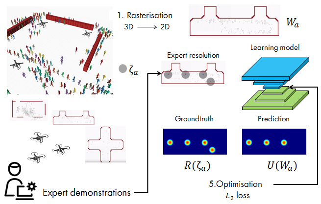
To do so, we define a learning model that takes an overhead image of an infrastructure and outputs a 2D utility function of which maxima are optimal sensor placements according to the expert. Figure 1 illustrates our approach on a simulated crowd for which Wi-Fi UAVs provide an internet connection. We choose a Convolutional Neural Network (CNN) to represent our utility function generator as it can process raw visual information contrary to other models that require hand-crafted features. We rely on Learning from Demonstration (LfD) [2] to train the CNN and Figure 2 illustrates the optimization: we compare the local maxima of the CNN utility function together with the expert locations and penalize the network proportionally to how far they are from each other. The CNN constrains us to do so in a differentiable way so we introduce an original regression loss. We simplify this learning into a simple regression problem with an astute projection of the expert locations into a 2D Gaussians. The penalty can then be estimated with a simple differentiable Mean-Square-Error (MSE) loss between this map and the CNN output. This conversion is inspired by the expert demonstration representation in visual attention model [4] (section II-B).
Our method is tested in a crowd simulator in which we add a simple wireless communication model. We choose two coverage strategies and implement an expert oracle to generate sensor location examples. Our approach reaches the same Quality of Service (QoS) as the oracles on both strategies. We also show that our method is not specific to the input data representation and solve two building monitoring problems based on the AGP and the Fortress Problem (FP).
Our contribution lies in the optimization method to learn a utility function only from demonstrations to solve sensor placement problems under constraints. This proof of concept targets the definition of the data representation and the learning optimisation. It is part of the global effort aiming at relieving the expert from modeling the coverage mission and explicitly defining a complex utility function.
II Problem Formulation
This section frames the sensor placement optimization in deep learning from demonstration. Given a 2D representation of the UAV mission, our model generates a utility function of which maxima are the UAV locations. These locations are chosen so as to mimic the network expert placements. To do so, the model is trained on examples of optimal sensor placements that the network expert provides.
II-A The Learning Problem Definition
Let be a UAV mission rasterised into a 2D map and be the expert locations on . We endeavor to learn a utility function generator on mission instances so that the maxima of the utility function are :
| (1) |
We choose to represent with a CNN as it is a non-linear function with a powerful representation space and can process raw images contrary to other models that require hand-crafted features. One constraint of the CNN is that its loss function must be differentiable. An intuitive loss is to measure how well the expert and learned locations and align. To do so, we first need to compute i.e. ’s maxima. Then we solve the assignment problem between and to assign each location in to the nearest expert location in . Finally, the loss is the Euclidean loss between the pairs assigned in the previous step. However, neither the argmax operation nor the assignment optimization are differentiable operations. Another difficulty comes from the varying number of maxima which is common to any learning problem with a list for output. Also, a trivial solution is to put sensor everywhere, which we want to avoid. To answer all these challenges, we define an alternative differentiable loss that still follows this intuitive behavior and casts the learning problem as a simple regression.
II-B The Loss Definition
We define a differentiable loss that penalizes the CNN with respect to how far matching locations in and are. It must meet the following requirements:
- •
must be differentiable.
- •
must be an increasing function of the euclidean distance between matching location pairs in .
- •
Modularity condition: ’s minimization residue decreases as has more maxima.
To do so, we convert an expert demonstration into a saliency map : for each location in , we draw an unnormalized Gaussian of mean and variance around each expert position (Figure 2: ). This constrains the CNN to also produce a saliency map with high peaks at sensor locations. The training loss then measures the distance from the expert saliency map to the CNN one :
| (2) |
This loss can be interpreted as ‘how well and align’. The conversion of into a saliency map is inspired by the visual attention model data representations [4]. As for the loss definition, it is motivated by the expert resolution of the task that can be cast as a submodular function optimization:
| (3) |
The submodularity property means that for a set of positions and such that , a new position :
| (4) |
Intuitively, this diminishing-return condition means that the more sensors one places, the less additional information the new sensor provides. An example of the submodularity condition is the following: let and a set of maxima. If the model produces a new maxima , the loss diminishes more if one starts from than when starting from .
Regarding the tuning of the parameter, the Gaussian variance must be small enough so that the map is only maximal at with no residual local maxima. Also, the smaller the variance, the higher is the penalty when the utility function misses a maxima or places it far from . However, a too small creates wide areas where the penalty signal is not informative enough for the network to learn. So must also be high enough to create a non-null learning signal everywhere to avoid that the model gets stuck between two expert sensor locations. A solution is to use two Gaussians: a first one with a small variance and a high amplitude which goal is to penalize misplaced maxima. And a second Gaussian with a higher variance and a smaller amplitude to strengthen the learning signal and guide maxima that are far from towards them. The loss now depends on four parameters :
| (5) |
In practice, we set . Then we perform a grid search to choose . The grid search range depends on the expert solution distribution: in general, are smaller when the mission usually requires more sensors. We assume that there may be several solutions for one task but only one solution strategy. The incorporation of multiple strategies is not addressed here.
II-C Utility Function as a Convolutional Neural Network
This section details the representation of the utility function generator . It is modeled by a convolutional neural network (CNN) with an encoder-decoder structure. It can learn from raw visual data and avoids the design of hand-crafted features. CNN are made of a composition of filter banks trained to extract relevant features. The only learning signal it needs to train is the expected output of the CNN. In this case, it is the rasterised expert solutions .
The encoder-decoder CNN structure is divided in two parts. The encoding part (Figure 2, blue) of the network is made of multiple filter banks interleaved with max-pooling layers that reduce the spatial dimension while keeping the most relevant features. The output of the encoder is the summary of the input features at multiple scales. It is fed to a decoder (Figure 2, green) which generates a utility function out of the learned relevant features. The decoder is also made of filter banks but they are interleaved with upsampling layers [16] so that the output of the decoder have the same spatial dimension as the input. In the decoder, the filters banks are transpose convolutions [6] that computes an embedding of the relevant features into a utility function.
The filter size and the number of layers in the encoder must be set together so that the scope of the last encoding layers covers the entire spatial dimension of the input. For an input image of size 64 pixels and max-pool layers every two convolutional layers, this can be achieved with a filter size of 3 and 4 convolutional layers. We advise to use the minimum number of encoding layers as possible since the bigger the network, the more expert demonstration you need to train it without overfitting. Also in practice, we observe that a bigger network may not even converge. Another good practice is to use a stack of small kernel filters rather than one big kernel filter [14].
Once the encoding part is set, there are two possible ways to decode: either make a heavy decoder symmetric to the encoder [3] or make a light decoder of only upsampling layers, one for each pooling layer in the encoder. The heavy decoder uses much more bank filters than the second but may be relevant for task with highly informative inputs which need more filters to extract all the relevant features. The light decoder proves to be enough to learn on our two use cases.
| Encoder | 2 conv-32 | P | 2 conv-64 | P | 2 conv-128 |
| Decoder | 1 conv-32T | UP | 1 conv-64T | UP | 1 conv-128T |
We note the composition of banks of 2D convolution filters, and when we use transpose-convolutions [6]. The max-pooling and upsampling layers [16] are designated by ‘P’ and ‘U’ respectively. The encoder and decoder architectures are summarized in Table I.
| Wi-Fi | Monitoring | |
| Train set size | 5000 | 25000 |
| Test set size | 800 | 1000 |
| image size | 256 | 64 |
| Batch size | 10 | 64 |
| Train epochs | 500 | 300 |
| Training duration | 6h | 4h |
III Experiments
This section describes the simulation and the training.
III-A UAV Wireless Network Simulation
A simple communication model is defined within the Pedsim 11 1 http://pedsim.silmaril.org/ crowd simulator wrapped in the Pedsim-ROS package 22 2 https://github.com/srl-freiburg/pedsim. We generate fake scenarios by defining random obstacles and waypoints for agents and run the simulation (Figure 3). The drones are equipped with a wireless AC card with a maximum throughput of 200Mbps, a signal range of 30m, and an emission power signal of 13dbm. These are standard values for Wi-Fi routers. The end receptor power sensitivity is set to -65dbm, which is enough to stream videos and run VoIp calls with a smartphone. We approximate the free-space path loss with an unnormalized Gaussian after rescaling the power signal from [-65dbm, 13dbm] to [0.1, 1]. is computed so that the signal power at =30m is 0.1 so .

We define two UAV deployment strategies summarized in Table III. The first one should place the UAVs to cover the maximum number of agents without regards to the end-user throughput bandwidth. The second one should cover the maximum number of agents under the constraint of providing them with a minimum of 5Mbps throughput, which is more than enough to watch Netflix with ultra HD quality. In both cases, the expert deploys a drone only if there is a cluster with more than 30 end-users without network access. We ignore other communication network related issues addressed [8] to focus only the placement problem.
| Strategy 1 (S1) | Strategy 2 (S2) |
|---|---|
| Maximum number of UAV: 10 | |
| Minimum size of group worth covering: 30 | |
| - | bandwidth |
III-B UAV Monitoring Simulation

In addition to the communication coverage above, we show that our method is restricted by neither the input data representation nor by the expert utility. To this end, we test it on a buliding monitoring task with UAV networks. We simulate the buildings with random polygons and emulate two experts with the famous Art-Gallery-Problem (AGP) and Fortress-Problem (FP) solutions (Figure 4). These two sensor placement problems pertain to a broad category of problems named Next-Best-View (NBV) problems. They arise in many applications among which autonomous robotic exploration, environment monitoring and inspection. In AGP, the expert places the minimum number of UAV-guards to always monitor the interior of an art gallery and catch potential thieves. In FP, the expert deploys the minimum number of guards outside of a fortress to constantly watch its perimeter. More generally, we optimize a visibility coverage function while minimizing the number of guards. For both missions, buildings are modeled with random polygons [5] and the expert solutions are computed with the numerical solver [15]. In this context, (eq. 1) is a polygon drawing on a pixels map.
III-C Evaluation
We introduce a generic metric to evaluate the utility function generator : the correspondence ratio. It measures the proportion of expert locations matched by the placements from the learned policy. We define matching locations as follow: we first solve the assignment problem between and , and note the resulting location pairs . Let , and match when , with a distance threshold specific to the task dimension. We set at 10% of the mission dimension and define the correspondence ratio as . We control whether generates trivial solutions with a score inspired from the precision metric in classification, hence the score name we use. We note the subset of that match no expert sensor locations and define the precision as . The score is 100% when the learned placements match exactly the expert ones with no additional locations then it decreases as the number of maxima increases.
Contrary to the training loss, we do not penalize if has more maxima than the expert solution . In practice, we observe that these additional maxima are other valid solution for the task. This metric is completed with task specific metric such as QoS. In the first strategy of the Wi-Fi UAV simulation, we measure the QoS with the proportion of end-users covered by the Wi-Fi network. For the second Wi-Fi UAV strategy, we also require the end-users’s throughput i.e. the amount of data received per second, to be higher than 5Mbps. As for the monitoring problems, the ‘QoS‘ is the ratio of buildings for which perfect coverage is reached. The expert always generates UAV locations that reach a correspondence ratio and QoS of 100%.
IV Results
The learned UAV placements and , the expert’s ones, have at least 75% of correspondences for all simulations. Positions correspond if they are closer than 10% of the simulation dimensions. There is substantial room for improvement regarding the exact matching of learned positions (25%). However, the QoS metrics suggest that although the learned locations differ from the expert ones, they are still valid deployment strategy and offer high QoS. Indeed, for all simulations, the QoS is higher than the correspondence ratio which shows that when the learned utility function does not mimic exactly the expert’s one, its maxima are an alternative valid solutions to the sensor placement problem. We study the influence of the learning parameter and observe that it improves the correspondence ratio up to 29%.
IV-A UAV Wi-Fi network
| Strategy | Corresp. (%) | QoS (%) | Precision (%) |
|---|---|---|---|
| UAV 1 | 75 | 100 | 75 |
| UAV 2 | 89 | 93 | 72 |
The correspondence ratio is above 75% for both UAV deployment strategies. It even reaches 89% for the second one where placements are additionally constrained with the end-user throughput. This supports the hypothesis that embeds the expert knowledge on the UAV placement and aims at imitating it as much as possible.
We also observe that the QoS is always higher than the correspondence ratio which shows that even when and do not match, still is a valid solution. This reinforces the hypothesis that can not only imitate the expert, but it can also provide alternative solutions while still abiding by the expert utility it learnt. Thus, the learned deployment still completes the mission even when it is different from the expert’s one. For the first strategy, 100% of the clusters with more than 30 end-users are covered even though the learned placements match only 75% of the expert’s ones. The model trained on the second strategy also covers all end-users clusters and misses the throughput requirement for only 7% of the end-users. Qualitatively, we observe that the utility function tends to either have maxima that match exactly the expert or produce a higher number maxima. It is up to the non-maxima-suppression step () to then filter utility maxima among those proposed.

Figure 5 shows the average throughput per agent over time during one dynamic scene for the expert (green) and the learned placement (blue). We observe that the learned placements produce a throughput pattern that follows the one generated with expert sensor locations. This suggests that not only embeds the expert utility function a time but also its dynamics.
IV-B UAV Monitoring Network
| Strategy | Corresp. (%) | QoS (%) | Precision (%) |
|---|---|---|---|
| AGP | 91 | 97 | 82 |
| FP | 86 | 90 | 78 |
The model learnt on the monitoring demonstrations comforts the previous analysis. It reaches a correspondence ratio above 86% on both missions (Table V). This shows that the learning method can generalise to different data representations. It also suggests that can embed high-level concepts, such as coverage, even when the data holds only a few visual features. We compute the ‘QoS’ coverage as the ratio of buildings for which perfect coverage is reached. As with the previous simulation, the QoS is higher than the correspondence ratio. This strengthens the observation that even when maxima do not match the expert solution , they still provide another valid solution.
IV-C Tuning the Learning Signal: setting
 UAV 1:
-rise=21%
UAV 1:
-rise=21%
 AGP:
-rise=29%
AGP:
-rise=29%
 UAV 2:
-rise=20%
UAV 2:
-rise=20%
 FP:
-rise=22%
FP:
-rise=22%
Figure 6 shows the influence of the Gaussian parameter for the rasterisation of the expert solutions . When is high, is penalized for generating utility functions with maxima even slightly different that the expert UAV locations . This incites to strictly mimic the expert. However, when the maxima are far from the expert’s one, has no indication on how to improve because all the learning signal is restricted to the neighbourhood of . This can significantly slow down the training, especially at the beginning of the optimization, and even prevent convergence. As decreases, the loss is more tolerant with that differ from the exprt even though it can lead to lower correspondence ratio. However, it allows to better recover from wrong utility functions. Finally, there is an value above which the rasterisation of the expert placement can generate artificial maxima.
We run a grid search on with a step of 10 for both the Wi-Fi UAV and the monitoring UAV deployment problems. We call -rise the difference between the correspondence ratio for the worst (red) and the best (green) parameter. Overall, we observe a significant -rise of at least 20%, and up to 29% for the AGP. These results reiterate the importance of data representation in learning from demonstrations and shows that our loss definition ensures an efficient learning. Empirically, we observe that setting to the quarter of the average distance between expert positions leads to satisfying results.
V Conclusion
This paper shows how to leverage network experts previous efforts to automate UAV deployment following the same expert policy. We learn a utility function generator that autonomously learns relevant features for the expert when solving the UAV placement problem. It aims at generating an approximation of the expert’s untold utility function which maxima are the optimal UAV locations. To do so, it only relies on expert demonstrations made of UAV previous missions and the expert solution. We model this generator with a CNN for its representation space properties: the CNN can autonomously learn complex and high-dimensional features relevant to the learning task which alleviate the need to hand-craft them. This property allows the generation of utility function that can solve NP-hard problems such as the Art Gallery Problem.
This learning method is tested on two types of UAV applications: dynamic Wi-Fi networks and monitoring networks. Simulation experiments show that this method can recover the expert’s utility function without the need for the task model or the closed-form expression of the utility. In both applications, the UAV locations computed from the learned utility function match at least 75% of the expert’s demonstrations. When they do not, they are still valid solutions to complete the mission. This shows that the learned utility function generator not only mimics the network expert but it also embeds the expert’s untold utility to provide alternative valid solutions.
References
- [1] Abadi, M., Barham, P., Chen, J., Chen, Z., Davis, A., Dean, J., Devin, M., Ghemawat, S., Irving, G., Isard, M., et al. Tensorflow: a system for large-scale machine learning. In OSDI (2016), vol. 16, pp. 265–283.
- [2] Argall, B. D., Chernova, S., Veloso, M., and Browning, B. A survey of robot learning from demonstration. Robotics and autonomous systems 57, 5 (2009), 469–483.
- [3] Badrinarayanan, V., Kendall, A., and Cipolla, R. Segnet: A deep convolutional encoder-decoder architecture for image segmentation. IEEE transactions on pattern analysis and machine intelligence 39, 12 (2017), 2481–2495.
- [4] Borji, A., and Itti, L. State-of-the-art in visual attention modeling. IEEE transactions on pattern analysis and machine intelligence 35, 1 (2013), 185–207.
- [5] de Castro, P. M. M., Devillers, O., Hert, S., Hoffmann, M., Kettner, L., Schönherr, S., Tifrea, A., and Gimeno, M. Geometric object generators. In CGAL User and Reference Manual, 4.10 ed. CGAL Editorial Board, 2017.
- [6] Dumoulin, V., and Visin, F. A guide to convolution arithmetic for deep learning. arXiv preprint arXiv:1603.07285 (2016).
- [7] González-Banos, H. A randomized art-gallery algorithm for sensor placement. In Proceedings of the seventeenth annual symposium on Computational geometry (2001), ACM, pp. 232–240.
- [8] Guillen-Perez, A., Sanchez-Iborra, R., Cano, M.-D., Sanchez-Aarnoutse, J. C., and Garcia-Haro, J. Wifi networks on drones. In ITU Kaleidoscope: ICTs for a Sustainable World (ITU WT), 2016 (2016), IEEE, pp. 1–8.
- [9] Hayat, S., Yanmaz, E., and Muzaffar, R. Survey on unmanned aerial vehicle networks for civil applications: A communications viewpoint. IEEE Communications Surveys & Tutorials 18, 4 (2016), 2624–2661.
- [10] Kingma, D., and Ba, J. Adam: A method for stochastic optimization. arXiv preprint arXiv:1412.6980 (2014).
- [11] Krause, A., Singh, A., and Guestrin, C. Near-optimal sensor placements in gaussian processes: Theory, efficient algorithms and empirical studies. Journal of Machine Learning Research 9, Feb (2008), 235–284.
- [12] O’rourke, J. Art gallery theorems and algorithms, vol. 57. Oxford University Press Oxford, 1987.
- [13] Shewry, M. C., and Wynn, H. P. Maximum entropy sampling. Journal of applied statistics 14, 2 (1987), 165–170.
- [14] Simonyan, K., and Zisserman, A. Very deep convolutional networks for large-scale image recognition. arXiv preprint arXiv:1409.1556 (2014).
- [15] Tozoni, D. C., de Rezende, P. J., and de Souza, C. C. A practical iterative algorithm for the art gallery problem using integer linear programming. Optimization Online (2013).
- [16] Zeiler, M. D., Taylor, G. W., and Fergus, R. Adaptive deconvolutional networks for mid and high level feature learning. In Computer Vision (ICCV), 2011 IEEE International Conference on (2011), IEEE, pp. 2018–2025.