Lund jet images from generative and cycle-consistent adversarial networks
Abstract
We introduce a generative model to simulate radiation patterns within a jet using the Lund jet plane. We show that using an appropriate neural network architecture with a stochastic generation of images, it is possible to construct a generative model which retrieves the underlying two-dimensional distribution to within a few percent. We compare our model with several alternative state-of-the-art generative techniques. Finally, we show how a mapping can be created between different categories of jets, and use this method to retroactively change simulation settings or the underlying process on an existing sample. These results provide a framework for significantly reducing simulation times through fast inference of the neural network as well as for data augmentation of physical measurements.
pacs
12.38.-tQuantum chromodynamics and 07.05.MhNeural networks, fuzzy logic, artificial intelligence1 Introduction

One of the most common objects emerging from hadron collisions at particle colliders such as the Large Hadron Collider (LHC) are jets. These are loosely interpreted as collimated bunches of energetic particles arising from the interactions of quarks and gluons, the fundamental constituents of the proton Sterman:1977wj; Salam:2009jx. In practice, jets are usually defined through a sequential recombination algorithm mapping final-state particle momenta to jet momenta, with a free parameter defining the radius up to which separate particles are clustered into a single jet Ellis:1993tq; Dokshitzer:1997in; Cacciari:2008gp.
Because of the high energies involved in the collisions at the LHC, heavy particles such as vector bosons or top quarks are frequently produced with very large transverse momenta. In this boosted regime, the decay products of these objects can become so collimated that they are reconstructed as a single jet. An active field of research is therefore dedicated to the theoretical understanding of radiation patterns within jets, notably to distinguish their physical origins and remove radiation unassociated with the hard process Thaler:2008ju; Kaplan:2008ie; Ellis:2009su; Ellis:2009me; Plehn:2009rk; Thaler:2010tr; Larkoski:2013eya; Chien:2013kca; Cacciari:2014gra; Larkoski:2014gra; Moult:2016cvt; Dasgupta:2013ihk; Larkoski:2014wba; Komiske:2017ubm; Komiske:2017aww; Dreyer:2018tjj; Dreyer:2018nbf; Kasieczka:2019dbj; Carrazza:2019efs; Berta:2019hnj; Moreno:2019bmu. Furthermore, measurements of jet properties provide a unique opportunity for accurate comparisons between theoretical predictions and data, and can be used to tune simulation tools Fischer:2014bja or extract physical constants Bendavid:2018nar.
In recent years, there has also been considerable interest in applications of generative adversarial networks (GAN) goodfellow2014generative and variational autoencoders (VAE) DBLP:journals/corr/KingmaW13 to particle physics, where such generative models can be used to significantly reduce the computing resources required to simulate realistic LHC data deOliveira:2017pjk; Paganini:2017hrr; Paganini:2017dwg; Otten:2019hhl; Musella:2018rdi; Datta:2018mwd; Cerri:2018anq; DiSipio:2019imz; Butter:2019cae; SHiP:2019gcl. In this paper, we introduce a generative model to create new samples of the substructure of a jet from existing data. We use the Lund jet plane Dreyer:2018nbf, shown in figure 1, as a visual representation of the clustering history of a jet. This provides an efficient encoding of a jets radiation patterns and can be directly measured experimentally ATLAS:2019sol. The Lund jet image is used to train a Least Square GAN (LSGAN) DBLP:journals/corr/MaoLXLW16 to reproduce simulated data within a few percent accuracy. We compare a range of alternative generative methods, and show good agreement between the original jets generated with Pythia v8.223 Sjostrand:2014zea using fast detector simulation with Delphes v3.4.1 particle flow deFavereau:2013fsa and samples provided by the different models DBLP:conf/icml/ArjovskyCB17. Finally, we show how a cycle-consistent adversarial network (CycleGAN) CycleGAN2017 can be used to create mappings between different categories of jets. We apply this framework to retroactively change the parameters of the parton shower on an event, adding non-perturbative effects to an existing parton-level sample, and transforming quark and gluon jets to a boosted sample.
These methods provide a systematic tool for data augmentation, as well as reductions of simulation time and storage space by several orders of magnitude, e.g. through a fast inference of the neural network with hardware architectures such as GPUs and field-programmable gate arrays (FPGA) Duarte:2018ite. The code frameworks and data used in this work are available as open-source and published material in frederic_dreyer_2019_3384921; frederic_dreyer_2019_3384919; gLund_data11 1 The codes are available at https://github.com/JetsGame/gLund and https://github.com/JetsGame/CycleJet.
2 Generating jets
In this article we will construct a generative model, which we call gLund, to create new samples of radiation patterns of jets. We first introduce the basis used to describe a jet as an image, then construct a generative model which can be trained on these objects.
2.1 Encoding radiation patterns with Lund images
To describe the radiation patterns of a jet, we will use the primary Lund plane representation Dreyer:2018nbf, which can be projected onto a two-dimensional image that serves as input to a neural network.
The Lund jet plane is constructed by reclustering a jet’s constituents with the Cambridge-Aachen (C/A) algorithmDokshitzer:1997in; Wobisch:1998wt. This algorithm sequentially recombines pairs of particles that have the minimal value, where and are the rapidity and azimuth of particle .
This clustering sequence can be used to construct an pixel image describing the radiation patterns of the initial jet. We iterate in reverse through the clustering sequence, labelling the momenta of the two branches of a declustering as and , ordered in transverse momentum such that . This procedure follows the harder branch and at each step we activate the pixel on the image corresponding to the coordinates , where is the transverse momentum of particle relative to .22 2 For simplicity, we consider only whether a pixel is on or off, instead of counting the number of hits as in Dreyer:2018nbf. While these two definitions are equivalent only for large image resolutions, this limitation can easily be overcome e.g. by considering a separate channel for each activation level.
2.2 Input data
The data sample used in this article consists of 500k jets, generated
using the dijet process in Pythia
v8.223.
Jets are clustered using the anti-
algorithm Cacciari:2008gp; Cacciari:2011ma with radius ,
and are required to pass a selection cut, with transverse momentum
GeV and rapidity .
Unless specified otherwise, results use the
Delphes v3.4.1 fast detector simulation,
with the delphes_card_ CMS_NoFastJet.tcl card to simulate both
detector effects and particle flow reconstruction.
The simulated jets are then converted to Lund images with pixels each using the procedure described in section 2.1. A pixel is set to one if there is a corresponding primary declustering sequence, otherwise it is left at zero.
The full samples used in this article can be accessed online gLund_data.
2.3 Probabilistic generation of jets

Generative adversarial networks NIPS2014_5423 are one of the most successful unsupervised learning methods. They are constructed using both a generator and discriminator , which are competing against each other through a value function .
In practice, we found improved performance when using a Least Square Generative Adversarial Network (LSGAN) DBLP:journals/corr/MaoLXLW16, a specific class of GAN which uses a least squares loss function for the discriminator, and has objective functions defined as
| (1) |
| (2) |
where we defined as a prior on input noise variables, and , and are the labels for the fake, real and presumed fake data respectively. Thus is trained in order to maximise the probability of correctly distinguishing the training examples and the samples from , following equation (1), while the latter is trained to minimise equation (2). The generator’s distribution optimises equation (2) when , so that the generator learns how to generate new samples from . The main advantage of the LSGAN over the original GAN framework is a more stable training process, due to an absence of vanishing gradients. In addition, we include a minibatch discrimination layer DBLP:journals/corr/SalimansGZCRC16 to avoid collapse of the generator.
The LSGAN is trained on the full sample of QCD Lund jet images. In order to overcome the limitation of GANs due to the sparse and discrete nature of Lund images, we will use a probabilistic interpretation of the Lund images to train the model. To this end, we will first re-sample our initial data set into batches of and create a new set of 500k images, each consisting of the average of initial input images, as shown in figure 2. These images can be reinterpreted as physical events through a random sampling, where the pixel value is interpreted as the probability that the pixel is activated. The value is a parameter of the model, with a large value leading to increased variance in the generated images compared to the reference sample, while for too low values the model performs poorly due to the sparsity and discreteness of the data. A further data preprocessing step before training the LSGAN consists in rescaling the pixel intensities to be in the range, and masking entries outside of the kinematic limit of the Lund plane. The images are then whitened using zero-phase components analysis (ZCA) whitening BELL19973327.
2.4 gLund model results
The optimal choice of hyperparameters, both for the LSGAN model architecture and for the image preprocessing, is determined using the distributed asynchronous hyperparameter optimisation library hyperopt Bergstra:2013:MSM:3042817.3042832.
The performance of each setup is evaluated by a loss function which compares the reference preprocessed Lund images to the artificial images generated by the LSGAN model. We define the loss function as
| (3) |
where is the norm of the difference between the average of the images of the two samples and is the absolute difference in structural similarity 1284395 values between 5000 random pairs of reference samples, and reference and generated samples.
We perform 1000 iterations and select the one for which the loss is minimal. In figure 3 we show some of the results obtained with the hyperopt library through the Tree-structured Parzen Estimator (TPE) algorithm. The LSGAN is constructed from a generator and discriminator. The generator consists in three dense layers with 512, 1024 and 2048 units respectively using LeakyReLU Maas13rectifiernonlinearities activation functions and batch normalisation layers, as well as a final layer matching the output dimension and using a hyperbolic tangent activation function. The discriminator is constructed from two dense layers with 768 and 384 units using a LeakyReLU activation function, followed by another 24-dimensional dense layer connected to a minibatch discrimination layer, with a final fully connected layer with one-dimensional output. The best parameters for this model are listed in table 1. The loss of the generator and discriminator networks of the LSGAN is shown in figure 4 as a function of training epochs.
In figure 5, the first two images illustrate an example of input image before and after preprocessing while the last two images represent the raw output from the LSGAN model and the corresponding sampled Lund image.

A selection of preprocessed input images and images generated with the LSGAN model are shown in figure 6. The final averaged results for the Lund jet plane density are shown in figure 7 for the reference sample (left), the data set generated by the gLund model (centre) and the ratio between these two samples (right). We observe a good agreement between the reference and the artificial sample generated by the gLund model. The model is able to reproduce the underlying distribution to within a 3-5% accuracy in the bulk region of the Lund image. Larger discrepancies are visible at the boundaries of the Lund image and are due the vanishing pixel intensities. In practice this model provides a new approach to reduce Monte Carlo simulation time for jet substructure applications as well as a framework for data augmentation.


Parameters Value Architecture LSGAN units 384 units 512 0.129 0.477 Aux ratio 12 Kernel dimension 1 Number of kernels 2 Minibatch discriminator Yes Epochs 5000 Batch size 32 Latent dimension 500 ZCA Yes 32 Learning rate Decay Optimiser Adagrad
2.5 Comparisons with alternative methods
Let us now quantify the quality of the model described in section 2.3 more concretely. As alternatives, we consider a variational autoencoder (VAE) DBLP:journals/corr/KingmaW13; DBLP:journals/corr/HigginsMGPUBML16; DBLP:journals/corr/abs-1804-03599 and a Wasserstein GAN DBLP:conf/icml/ArjovskyCB17; DBLP:journals/corr/GulrajaniAADC17.
A VAE is a latent variable model, with a probabilistic encoder , and a probabilistic decoder to map a representation from a prior distribution . The algorithm learns the marginal likelihood of the data in this generative process, which corresponds to maximising
| (4) |
where is an adjustable hyperparameter controlling the disentanglement of the latent representation . In our implementation, we will set , which corresponds to the original VAE framework.
During the training of the VAE, we use KL cost annealing DBLP:journals/corr/BowmanVVDJB15 to avoid a collapse of the VAE output to the prior distribution. This is a problem caused by the large value of the KL divergence term in the early stages of training, which is mitigated by adding a variable weight to the KL term in the cost function, expressed as
| (5) |
Finally, we will also consider a Wasserstein GAN with gradient penalty (WGAN-GP). WGANs DBLP:conf/icml/ArjovskyCB17 use the Wasserstein distance to construct the value function, but can suffer from undesirable behaviour due to the critic weight clipping. This can be mitigated through gradient penalty, where the norm of the gradient of the critic is penalised with respect to its input DBLP:journals/corr/GulrajaniAADC17.
We determine the best hyperparameters for both of these models through a hyperopt parameter sweep, which is summarised in Appendix A. To train these models using Lund images, we then use the same preprocessing steps described in section 2.3.
To compare our three models, we consider two slices of fixed or size, cutting along the Lund jet plane horizontally or vertically respectively.
In figure 8, we show the slice, with the reference sample in red. The lower panel gives the ratio of the different models to the reference Pythia 8 curve, showing very good performance for the LSGAN and WGAN-GP models, which are able to reproduce the data within a few percent. The VAE model also qualitatively reproduces the main features of the underlying distribution, however we were unable to improve the accuracy of the generated sample to more than without avoiding the issue of posterior collapse. The same observations can be made in figure 9, which shows the Lund plane density as a function of , for a fixed slice in .
In figure 10a we show the distribution of the number of activated pixels per image for the reference sample generated with Pythia 8 and the artificial images produced by the LSGAN, WGAN-GP and VAE models. All models except the VAE model provide a good description of the reference distribution.
We also use the Lund image to reconstruct the soft-drop multiplicity Frye:2017yrw. To this end, for a simpler correspondence between this observable and the Lund image, we retrained the generative models using as -axis. The soft-drop multiplicity can then be extracted from the final image, and is shown in figure 10b for each model using and . The dashed lines indicate the true reference distribution, as evaluated directly on the declustering sequence, and which differs slightly from the reconstructed curve due to the finite pixel and image size.
Finally, in figure 10c, we show the reconstructed mass of the groomed jet using the modified Mass Drop Tagger Dasgupta:2013ihk with , where we approximate the mass as
| (6) |
The dotted line shows the true mass distribution, evaluated with the left-hand side of equation (6) on the groomed jet. As in previous comparisons, we observe a very good agreement of the LSGAN and WGAN-GP models with the reference sample.
We note that while the WGAN-GP model is able to accurately reproduce the distribution of the training data, as discussed in Appendix A, the individual images themselves can differ quite notably from their real counterpart. For this reason, our preferred model in this paper is the LSGAN-based one.
3 Reinterpreting events using domain mappings
In this section, we will introduce a novel application of domain mappings to reinterpret existing event samples. To this end, we implement a cycle-consistent adversarial network (CycleGAN) CycleGAN2017, which is an unsupervised learning approach to create translations between images from a source domain to a target domain.
Using as input Lund images generated through different processes or generator settings, one can use this technique to create mappings between different types of jet. As examples, we will consider a mapping from parton-level to detector-level images, and a mapping from QCD images generated through Pythia 8’s dijet process, to hadronically decaying jets obtained from scattering.
The cycle obtained for a CycleGAN trained on parton and detector-level images is shown in figure 11, where an initial parton-level Lund image is transformed to a detector-level one, before being reverted again. The sampled image is shown in the bottom row.

3.1 CycleGANs and domain mappings
A CycleGAN learns mapping functions between two domains and , using as input training samples from both domains. It creates an unpaired image-to-image translation by learning both a mapping and an inverse mapping which observes a forward cycle consistency as well as a backward cycle consistency . This behaviour is achieved through the implementation of a cycle consistency loss
| (7) |
Additionally, the full objective includes also adversarial losses to both mapping functions. For the mapping function and its corresponding discriminator , the objective is expressed as
| (8) |
such that is incentivized to generate images that resemble images from , while the discriminator attempts to distinguish between translated and original samples.
Thus, CycleGAN aims to find arguments solving
| (9) |
where is the full objective, given by
| (10) |
Here is parameter controlling the importance of the cycle consistency loss. We implemented a CycleGAN framework, labelled CycleJet, that can be used to create mappings between two domains of Lund images.33 3 CycleJet can also be used for similar practical purposes as DCTR Andreassen:2019nnm, albeit it is of course limited to the Lund image representation. By training a network on parton and detector-level images, this method can thus be used to retroactively add non-perturbative and detector effects to existing parton-level samples. Similarly, one can train a model using images generated through two different underlying processes, allowing for a mapping e.g. from QCD jets to or top initiated jets.
3.2 CycleJet model results
Following the pipeline presented in section 2.4 we perform 1000 iterations of the hyperparameter scan using the hyperopt library and the loss function
| (11) |
where and indexes refer to the desired input and output samples respectively so and are the average reference images before the CycleGAN transformation while and correspond to the average image after the transformation. Furthermore, for this model we noticed better results when preprocessing the pixel intensities with the standardisation procedure of removing the mean and scaling to unit variance, instead of a simpler rescaling in the [-1,1] range as done in section 2.
Parameters Value filters 32 filters 32 cycle 10 identity factor 0.2 Epochs 3 Batch size 128 ZCA Yes 20 Learning rate Decay 0.7 Optimiser Adam
The CycleJet model consists in two generators and two discriminators. The generators consist in a down-sampling module with three two-dimensional convolutional layers with 32, 64 and 128 filters respectively, and LeakyReLU activation function and instance normalisation DBLP:journals/corr/UlyanovVL16, followed by an up-sampling with two two-dimensional convolutional layers with 64 and 32 filter. The last layer is a two-dimensional convolution with one filter and hyperbolic tangent activation function. The discriminators take three two-dimensional convolutional layers with 32, 64 and 128 filters and LeakyReLU activation. The first convolutional layer has additionally an instance normalisation layer and the final layer is a two-dimensional convolutional layer with one filter. The best parameters for the CycleJet model are shown in table 2.
In the first row of figure 12 we show results for an initial average parton-level sample before (left) and after (right) applying the parton-to-detector mapping encoded by the CycleJet model, while in the second row of the same figure we perform the inverse operation by taking as input the average of the dephes-level sample before (left) and after (right) applying the CycleJet detector-to-parton mapping. This example shows clearly the possibility to add non perturbative and detector effects to a parton level simulation within good accuracy. Similarly to the previous example, in figure 13 we present the mapping between QCD-to- jets and vice-versa. Also in this case, the overall quality of the mapping is reasonable and provides and interesting successful test case for process remapping.
For both examples we observe a good level agreement for the respective mappings, highlighting the possibility to use such an approach to save CPU time for applying full detector simulations and non perturbative effects to parton level events. It is also possible to train the CycleJet model on Monte Carlo data and apply the corresponding mapping to real data.


4 Conclusions
We have conducted a careful study of generative models applied to jet substructure.
First, we trained a LSGAN model to generate new artificial samples of detector level Lund jet images. With this, we observed agreement to within a few percent accuracy in the bulk of the phase space with respect to the reference data. This new approach provides an efficient method for fast simulation of jet radiation patterns without requiring the long runtime of full Monte Carlo event generators. Another advantage consists in the possibility of this method to be applied to real collider data to generate accurate physical samples, as well as making it possible to avoid the necessity for large storage space by generating realistic samples on-the-fly.
Secondly, a CycleGAN model was constructed to map different jet configurations, allowing for the conversion of existing events. This procedure can be used to change Monte Carlo parameters such as the underlying process or the shower parameters. As examples we show how to convert an existing sample of QCD jets into jets and vice-versa, or how to add non perturbative and detector effects to a parton level simulation. As for the LSGAN, this method can be used to save CPU time by including full detector simulations and non perturbative effects to parton level events. Additionally, one could use CycleJet to transform real data using mappings trained on Monte Carlo samples or apply them to samples generated through gLund.
To achieve the results presented in this paper we have implemented a rather convolved preprocessing step which notably involved combining and resampling multiple images. This procedure was necessary to achieve accurate distributions but comes with the drawback of loosing information on correlations between emissions at wide angular and transverse momentum separation. Therefore, it is difficult to evaluate or improve the formal logarithmic accuracy of the generated samples. This limitation could be circumvented with an end-to-end GAN architecture more suited to sparse images. We leave a more detailed study of this for future work. The full code and the pretrained models presented in this paper are available in frederic_dreyer_2019_3384921; frederic_dreyer_2019_3384919.
Acknowledgments
We thank Sydney Otten for discussions on -VAEs. We also acknowledge the NVIDIA Corporation for the donation of a Titan Xp GPU used for this research. F.D. is supported by the Science and Technology Facilities Council (STFC) under grant ST/P000770/1. S.C. is supported by the European Research Council under the European Union’s Horizon 2020 research and innovation Programme (grant agreement number 740006).
Appendix A VAE and WGAN-GP models
In this appendix we present the final parameters as well as generated event samples for the VAE and WGAN-GP models used in section 2.5. These models are obtained after applying the hyperopt procedure described in section 2.4.
Parameters Value Intermediate dimension 384 KL annealing rate 0.25 KL annealing factor 1.05 Minibatch discriminator No Epochs 50 Batch size 32 Latent dimension 1000 ZCA Yes 32 Learning rate Decay 0.9 Optimiser Adam
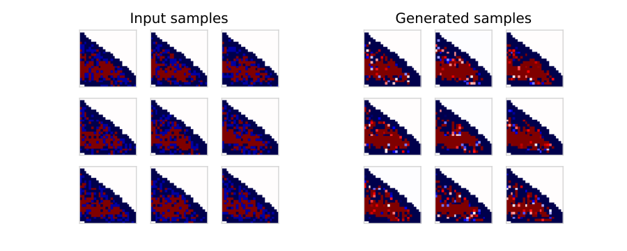
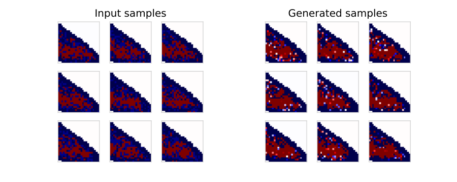
The VAE encoder consists of a dense layer with 384 units with ReLU activation function connected to a latent space with 1000 dimensions. The decoder consists of a dense layer with 384 units with ReLU activation followed by an output layer which matches the shape of the images and has a hyperbolic tangent activation function. The reconstruction loss function used during training is taken to be the mean squared error. The best parameters for the VAE model obtained after the hyperopt procedure are shown in table 3. In figure 14 we show a random selection of preprocessed images generated through the VAE. From a qualitative point of view the images appear realistic on an event-by-event comparison however as highlighted in section 2.5, the VAE model does not reproduce the underlying distribution accurately.
Parameters Value units 16 units 4 0.3 Dropout 0.15 momentum 0.7 momentum 0.7 Minibatch discriminator No Epochs 300 Batch size 32 Latent dimension 800 ZCA Yes 32 Learning rate Decay 0.9 Optimiser RMSprop

Finally, the WGAN-GP consists in a generator and discriminator. The generator architecture contains a dense layer with 1152 units with ReLU activation function followed by three sequential two-dimensional convolutional layers with a kernel size of 4 and respectively 32, 16 and 1 filters. Between these layers we apply batch normalisation and ReLU activation function while the final layer has a hyperbolic tangent activation function. On the other hand, the discriminator is composed by 4 two-dimensional convolutional layers with a kernel size of 3 and respectively 16, 32, 64, 128 and 128 filters. We apply batch normalisation for the last three layers and all of them LeakyReLU activation function with a dropout layer. In table 4 we provide the best parameters of the WGAN-GP model, always obtained through the hyperopt scan procedure. In figure 15 we show a random selection of preprocessed images generated through the WGAN-GP. Due to the convolutional filters of this model the preprocessing differs slightly from the description in section 2.3 as we do not remove pixels outside the kinematic range resulting in images with non zero background pixels. While distributions presented in section 2.5 are in good agreement with data, it is clear that for this WGAN-GP model the individual images look different from the input data.
References
- (1) G.F. Sterman, S. Weinberg, Phys. Rev. Lett. 39, 1436 (1977)
- (2) G.P. Salam, Eur. Phys. J. C67, 637 (2010), 0906.1833
- (3) S.D. Ellis, D.E. Soper, Phys. Rev. D48, 3160 (1993), hep-ph/9305266
- (4) Y.L. Dokshitzer, G.D. Leder, S. Moretti, B.R. Webber, JHEP 08, 001 (1997), hep-ph/9707323
- (5) M. Cacciari, G.P. Salam, G. Soyez, JHEP 04, 063 (2008), 0802.1189
- (6) J. Thaler, L.T. Wang, JHEP 07, 092 (2008), 0806.0023
- (7) D.E. Kaplan, K. Rehermann, M.D. Schwartz, B. Tweedie, Phys. Rev. Lett. 101, 142001 (2008), 0806.0848
- (8) S.D. Ellis, C.K. Vermilion, J.R. Walsh, Phys. Rev. D80, 051501 (2009), 0903.5081
- (9) S.D. Ellis, C.K. Vermilion, J.R. Walsh, Phys. Rev. D81, 094023 (2010), 0912.0033
- (10) T. Plehn, G.P. Salam, M. Spannowsky, Phys. Rev. Lett. 104, 111801 (2010), 0910.5472
- (11) J. Thaler, K. Van Tilburg, JHEP 03, 015 (2011), 1011.2268
- (12) A.J. Larkoski, G.P. Salam, J. Thaler, JHEP 06, 108 (2013), 1305.0007
- (13) Y.T. Chien, Phys. Rev. D90, 054008 (2014), 1304.5240
- (14) M. Cacciari, G.P. Salam, G. Soyez, Eur. Phys. J. C75, 59 (2015), 1407.0408
- (15) A.J. Larkoski, I. Moult, D. Neill, JHEP 12, 009 (2014), 1409.6298
- (16) I. Moult, L. Necib, J. Thaler, JHEP 12, 153 (2016), 1609.07483
- (17) M. Dasgupta, A. Fregoso, S. Marzani, G.P. Salam, JHEP 09, 029 (2013), 1307.0007
- (18) A.J. Larkoski, S. Marzani, G. Soyez, J. Thaler, JHEP 05, 146 (2014), 1402.2657
- (19) P.T. Komiske, E.M. Metodiev, B. Nachman, M.D. Schwartz, JHEP 12, 051 (2017), 1707.08600
- (20) P.T. Komiske, E.M. Metodiev, J. Thaler, JHEP 04, 013 (2018), 1712.07124
- (21) F.A. Dreyer, L. Necib, G. Soyez, J. Thaler, JHEP 06, 093 (2018), 1804.03657
- (22) F.A. Dreyer, G.P. Salam, G. Soyez, JHEP 12, 064 (2018), 1807.04758
- (23) A. Butter et al., SciPost Phys. 7, 014 (2019), 1902.09914
- (24) S. Carrazza, F.A. Dreyer (2019), 1903.09644
- (25) P. Berta, L. Masetti, D.W. Miller, M. Spousta (2019), 1905.03470
- (26) E.A. Moreno, O. Cerri, J.M. Duarte, H.B. Newman, T.Q. Nguyen, A. Periwal, M. Pierini, A. Serikova, M. Spiropulu, J.R. Vlimant (2019), 1908.05318
- (27) N. Fischer, S. Gieseke, S. Plätzer, P. Skands, Eur. Phys. J. C74, 2831 (2014), 1402.3186
- (28) Les Houches 2017: Physics at TeV Colliders Standard Model Working Group Report (2018), 1803.07977
- (29) I. Goodfellow, J. Pouget-Abadie, M. Mirza, B. Xu, D. Warde-Farley, S. Ozair, A. Courville, Y. Bengio, Generative adversarial nets, in Advances in neural information processing systems (2014), pp. 2672–2680
- (30) D.P. Kingma, M. Welling, Auto-Encoding Variational Bayes, in 2nd International Conference on Learning Representations, ICLR 2014, Banff, AB, Canada, April 14-16, 2014, Conference Track Proceedings (2014), http://arxiv.org/abs/1312.6114
- (31) L. de Oliveira, M. Paganini, B. Nachman, Comput. Softw. Big Sci. 1, 4 (2017), 1701.05927
- (32) M. Paganini, L. de Oliveira, B. Nachman, Phys. Rev. Lett. 120, 042003 (2018), 1705.02355
- (33) M. Paganini, L. de Oliveira, B. Nachman, Phys. Rev. D97, 014021 (2018), 1712.10321
- (34) S. Otten, S. Caron, W. de Swart, M. van Beekveld, L. Hendriks, C. van Leeuwen, D. Podareanu, R. Ruiz de Austri, R. Verheyen (2019), 1901.00875
- (35) P. Musella, F. Pandolfi, Comput. Softw. Big Sci. 2, 8 (2018), 1805.00850
- (36) K. Datta, D. Kar, D. Roy (2018), 1806.00433
- (37) O. Cerri, T.Q. Nguyen, M. Pierini, M. Spiropulu, J.R. Vlimant, JHEP 05, 036 (2019), 1811.10276
- (38) R. Di Sipio, M. Faucci Giannelli, S. Ketabchi Haghighat, S. Palazzo (2019), 1903.02433
- (39) A. Butter, T. Plehn, R. Winterhalder (2019), 1907.03764
- (40) (2019), 1909.04451
- (41) T.A. collaboration (ATLAS) (2019)
- (42) X. Mao, Q. Li, H. Xie, R.Y.K. Lau, Z. Wang, CoRR abs/1611.04076 (2016), 1611.04076
- (43) T. Sjöstrand, S. Ask, J.R. Christiansen, R. Corke, N. Desai, P. Ilten, S. Mrenna, S. Prestel, C.O. Rasmussen, P.Z. Skands, Comput. Phys. Commun. 191, 159 (2015), 1410.3012
- (44) J. de Favereau, C. Delaere, P. Demin, A. Giammanco, V. Lemaître, A. Mertens, M. Selvaggi (DELPHES 3), JHEP 02, 057 (2014), 1307.6346
- (45) M. Arjovsky, S. Chintala, L. Bottou, Wasserstein Generative Adversarial Networks, in Proceedings of the 34th International Conference on Machine Learning, ICML 2017, Sydney, NSW, Australia, 6-11 August 2017 (2017), pp. 214–223, http://proceedings.mlr.press/v70/arjovsky17a.html
- (46) J.Y. Zhu, T. Park, P. Isola, A.A. Efros, Unpaired Image-to-Image Translation using Cycle-Consistent Adversarial Networkss, in Computer Vision (ICCV), 2017 IEEE International Conference on (2017)
- (47) J. Duarte et al., JINST 13, P07027 (2018), 1804.06913
- (48) F. Dreyer, S. Carrazza, Jetsgame/glund v1.0.0 (2019), https://doi.org/10.5281/zenodo.3384920
- (49) F. Dreyer, S. Carrazza, Jetsgame/cyclejet v1.0.0 (2019), https://doi.org/10.5281/zenodo.3384918
- (50) S. Carrazza, F.A. Dreyer, JetsGame/data v1.0.0 (2019), this repository is git-lfs., https://doi.org/10.5281/zenodo.2602514
- (51) M. Wobisch, T. Wengler, Hadronization corrections to jet cross-sections in deep inelastic scattering, in Monte Carlo generators for HERA physics. Proceedings, Workshop, Hamburg, Germany, 1998-1999 (1998), pp. 270–279, hep-ph/9907280
- (52) M. Cacciari, G.P. Salam, G. Soyez, Eur. Phys. J. C72, 1896 (2012), 1111.6097
- (53) I.J. Goodfellow, J. Pouget-Abadie, M. Mirza, B. Xu, D. Warde-Farley, S. Ozair, A. Courville, Y. Bengio, in Proceedings of the 27th International Conference on Neural Information Processing Systems - Volume 2 (MIT Press, Cambridge, MA, USA, 2014), NIPS’14, pp. 2672–2680, http://dl.acm.org/citation.cfm?id=2969033.2969125
- (54) T. Salimans, I.J. Goodfellow, W. Zaremba, V. Cheung, A. Radford, X. Chen, CoRR abs/1606.03498 (2016), 1606.03498
- (55) A.J. Bell, T.J. Sejnowski, Vision Research 37, 3327 (1997)
- (56) J. Bergstra, D. Yamins, D.D. Cox, Making a Science of Model Search: Hyperparameter Optimization in Hundreds of Dimensions for Vision Architectures, in Proceedings of the 30th International Conference on International Conference on Machine Learning - Volume 28 (JMLR.org, 2013), ICML’13, pp. I–115–I–123
- (57) Zhou Wang, A.C. Bovik, H.R. Sheikh, E.P. Simoncelli, IEEE Transactions on Image Processing 13, 600 (2004)
- (58) A.L. Maas, A.Y. Hannun, A.Y. Ng, Rectifier nonlinearities improve neural network acoustic models, in in ICML Workshop on Deep Learning for Audio, Speech and Language Processing (2013)
- (59) I. Higgins, L. Matthey, X. Glorot, A. Pal, B. Uria, C. Blundell, S. Mohamed, A. Lerchner, CoRR abs/1606.05579 (2016), 1606.05579
- (60) C.P. Burgess, I. Higgins, A. Pal, L. Matthey, N. Watters, G. Desjardins, A. Lerchner, CoRR abs/1804.03599 (2018), 1804.03599
- (61) I. Gulrajani, F. Ahmed, M. Arjovsky, V. Dumoulin, A.C. Courville, CoRR abs/1704.00028 (2017), 1704.00028
- (62) S.R. Bowman, L. Vilnis, O. Vinyals, A.M. Dai, R. Józefowicz, S. Bengio, CoRR abs/1511.06349 (2015), 1511.06349
- (63) C. Frye, A.J. Larkoski, J. Thaler, K. Zhou, JHEP 09, 083 (2017), 1704.06266
- (64) A. Andreassen, B. Nachman (2019), 1907.08209
- (65) D. Ulyanov, A. Vedaldi, V.S. Lempitsky, CoRR abs/1607.08022 (2016), 1607.08022