Stochastic quasi-Newton with line-search regularization
Abstract
In this paper we present a novel quasi-Newton algorithm for use in stochastic optimisation. Quasi-Newton methods have had an enormous impact on deterministic optimisation problems because they afford rapid convergence and computationally attractive algorithms. In essence, this is achieved by learning the second-order (Hessian) information based on observing first-order gradients. We extend these ideas to the stochastic setting by employing a highly flexible model for the Hessian and infer its value based on observing noisy gradients. In addition, we propose a stochastic counterpart to standard line-search procedures and demonstrate the utility of this combination on maximum likelihood identification for general nonlinear state space models.
keywords
Nonlinear System Identification, Stochastic Optimisation, Stochastic Gradient, Stochastic Quasi-Newton, Sequential Monte Carlo, Particle Filter, and Gaussian Process.footnoteinfo]This paper was not presented at any IFAC meeting. Corresponding author: A. Wills.
,
1 Introduction
We are interested in the non-convex stochastic optimisation problem
| (1) |
where we only have access to noisy evaluations of the cost function and its first-order derivatives. The problem has a long history and an important landmark development was the so-called stochastic approximation idea derived by Robbins and Monro almost 70 years ago [42]. The central idea of stochastic approximation is to form a Markov-Chain for via
| (2) |
that converges (under fairly mild conditions) to a local minimum of (1) for careful choices of the search-direction and step-length (see e.g. [7]).
In recent years the relevance of this problem has massively increased mainly due to the fact that it arises in at least the following two important situations. First, when the cost function and its gradients are intractable, but where we can still make use of numerical methods to compute noisy estimates (preferably unbiased) of these objects. Second, when the cost function inherently depends on a very large amount of data and it becomes impractical to evaluate it or the associated gradient using the entire dataset. It is then standard to use only a smaller fraction of the data, which is commonly referred to as minibatching. This situation arises in large-scale application of supervised machine learning and in particular in deep learning.
The application that motivated us to develop the solution presented in this work is that of maximum likelihood identification of nonlinear state space models. This is a specific instance of the first situation mentioned above. The cost function—the likelihood—is intractable, but we have numerical methods—sequential Monte Carlo (SMC) [18, 25, 49]—that provide unbiased estimates of the likelihood [11, 39]. For two relatively recent overviews of the use of SMC—a.k.a. particle filters—in nonlinear system identification, see [43, 22].
Our main contribution is a new stochastic optimisation algorithm which features mechanisms facilitating the use of second-order information (Hessian) in calculating the search-direction , and a stochastic line search to compute the step-length . The representation used for the Hessian is provided by the Gaussian process [41] and we develop a method for its online updating as the optimisation algorithm progresses. We also derive a stochastic line-search procedure that employs a version of the Armijo condition [2, 53, 54]. It is perhaps surprising that little work has been done when it comes to developing stochastic line-search methods [5]. We stress that while the developments mentioned above are generally applicable, the application that motivated us to undertake this work is the nonlinear system identification problem, which provides an important spin-off contribution.
2 Related work
Due to its importance, the stochastic optimisation problem is rather well studied by now. The first stochastic optimisation algorithm was introduced in [42]. It makes use of first-order information only, motivating the name stochastic gradient (SG), which is the contemporary term [7] for these algorithms, originally referred to as stochastic approximation. Interestingly most SG algorithms are not descent methods since the stochastic nature of the update can easily produce a new iterate corresponding to an increase in the cost function. Instead, they are Markov chain methods in that their update rule defines a Markov chain.
Since the landmark paper [42], many extensions and modifications have been developed within the statistics and automatic control communities. While the contributions are too many to enumerate here, some notable works include convergence results [23, 29, 30], online parameter estimation and system identification in [27, 28], adaptive control strategies [17], and general books in the area [4, 48, 31]. It is important to note that a primary motivation for the current paper is the closely related area of system identification for nonlinear dynamic systems.
This existing research is having an enormous impact in the related area of machine learning at present and we believe the reason is simple: it is used to solve almost all supervised machine learning problems, including all deep learning problems [7]. This is evidenced by all available toolboxes in the area offering SG algorithms and variants of them. Due to this, SG methods are still receiving enormous research attention.
The primary focus of current research activity is directed towards producing algorithms with improved convergence rates. Two important aspects that impact convergence rate are:
- •
Poor problem scaling can lead to slow convergence [7];
- •
Regarding the first point, a well-known drawback of first-order methods is that the choice of coordinate system can greatly impact the rate of convergence, which is highlighted in the concluding comments of a recent review paper on the topic [7]. Incorportating second-order information (Hessian) can alleviate the sensitivity to coordinate choice, which is one of the motivations for the Newton’s method and it’s locally quadratic convergence rate. At the same time, in many pratical situations, computing the Hessian is impractical, which is certainly the case in many system identification problems and almost all deep learning problems. Addressing this problem are the infamous suite of quasi-Newton methods such as the BFGS method [10, 13, 16, 47], Broyden’s method [8] and the DFP formula [15, 9]. In essence, these algorithms learn the Hessian (or its inverse) matrix based on first-order information, resulting in fast convergence and computationally attractive algorithms.
For the stochastic setting of the current paper, these classical quasi-Newton methods are not applicable [7]. Towards addressing this, over the past decade we have witnessed increasing capabilities of so-called stochastic quasi-Newton methods, the category to which our current developments belong. The work by [45] developed modifications of BFGS and its limited memory version. There has also been a series of papers approximating the inverse Hessian with a diagonal matrix, see e.g. [6] and [12]. The idea of exploiting regularisation together with BFGS was successfully introduced by [36]. Some of these approaches rely on the assumption that maintaining common random numbers between two gradient evaluations will result in locally deterministic behaviour. While this assumption may be satisfied for certain classes of functions, it is not valid of nonlinear system identification situation when SMC based calculation of the cost and gradient are employed [22].
In the current paper, we take a different approach and develop a new quasi-Newton algorithm that deals with the stochastic problem directly. The development stems from stating the integral form of the so-called quasi-Newton equation, where an exact relation between gradient differences and the Hessian are provided. This provides a natural point for treating the stochastic gradients and we then propose the use of a flexible model structure for the unknown Hessian matrix based on formulating the problem as a Gaussian Process regression problem. This results in a fully probabilistic model for the Hessian, where the mean function is used as a surrogate Hessian matrix in a new quasi-Newton algorithm.
Regarding the second point, the step-length schedule is also addressed in the current paper by suggesting a stochastic line-search procedure modelled after the backtracking line-search with Armijo conditions [2, 53, 54]. It is interesting—and perhaps somewhat surprising—to note that it is only very recently that stochastic line search algorithms have started to become available. One nice example is the approach proposed by [34] which uses the framework of Gaussian processes and Bayesian optimisation. The step length is chosen that best satisfies a probabilistic measure combining reduction in the cost function with satisfaction of the Armijo condition. Conceptually more similar to our procedure is the line search proposed by [5], which is tailored for problems that are using sampled mini-batches, as is common practice within deep learning. The final line-search algorithm proposed in the current paper begins with a more classical backtracking style procedure and converges towards a deterministic schedule that satisfies the typical convergence requirements for SG methods.
While we started this development in our earlier conference paper [52], that paper missed several key ingredients that we provide in this paper. In particular we have now developed a correct and properly working mechanism for representing and updating the local Hessian using a GP. Furthermore, we have introduced a completely new and improved line search algorithm.
3 Stochastic quasi-Newton method
Quasi-Newton methods have found enormous success within the field of optimisation [38]. The primary reasons are that they capture the cost function curvature information and that they are computationally inexpensive, requiring only gradient calculations. The curvature information leads to better scaling of the negative gradient direction and consequently to faster convergence [38].
In pursuit of similar advantages for the stochastic optimisation problem, many authors have considered how to develop quasi-Newton algorithms when the gradient vector is stochastic (see e.g. the concluding remarks in [7]). While the potential benefits of incorporating curvature information are widely recognised, it remains a rapidly evolving area.
In order to describe our quasi-Newton approach in Section 4, here we provide some background material with a slightly non-standard introduction to the quasi-Newton method (Section 3.1). This leads to the so-called quasi-Newton integral from which the more classic secant equation can be obtained. The secant equation is essential to all standard quasi-Newton methods such as BFGS, DFP and SR1 methods, and is obtained by introducing a rather strong approximation. We refrain from making this approximation and in Section 3.2 we show that we can formulate a stochastic version of the quasi-Newton integral.
3.1 A non-standard quasi-Newton introduction
The idea underlying the Newton and quasi-Newton methods is to learn a local quadratic surrogate model of the cost function around the current iterate
| (3) |
where . Note that (3) is a second-order Taylor expansion of , i.e. in a close vicinity around the current iterate .
Quasi-Newton methods are used in situations where the curvature information inherent in the Hessian is important at the same time as it is too expensive or impossible to compute the Hessian. The idea is to introduce a representation for the Hessian and compute an estimate of the Hessian using zero- and first-order information (function values and their gradients). More specifically the existing quasi-Newton methods are designed to represent the cost function according to the following model
| (4) |
for some matrix representing the Hessian.
In order to see how to update the Hessian approximation as the algorithm proceeds let us assume that and are known. The line segment connecting these two iterates can be expressed as
| (5) |
The fundamental theorem of calculus states that
| (6) |
and the chain rule allows us to express the integrand as
| (7) |
By inserting (7) into (6) we conclude that
| (8) |
We introduce the following notation
| (9) |
for the differences between two adjacent iterates. The integral (8) can be written in a more convenient form according to
| (10) |
which we will refer to as the quasi-Newton integral. The interpretation of the above development is that the difference between two consecutive gradients constitute a line integral observation of the Hessian. The challenge is that the Hessian is unknown and there is no functional form available for it.
The approach taken by existing quasi-Newton algorithms is to assume that the Hessian can be described by a zero-order Taylor expansion,
| (11) |
implying that the integral equation in (10) is approximated according to
| (12) |
This equation is known as the secant condition or the quasi-Newton equation [14, 38]. It constrains the possible choices for the Hessian approximation since in addition to being symmetric, it should at least satisfy the secant condition (12). This is still not enough to uniquely determine the Hessian and we are forced to include additional assumptions to find the Hessian approximation. Depending on which assumptions are made we recover the standard quasi-Newton algorithms. See [20] for additional details.
Our approach is fundamentally different in that we will allow the Hessian to evolve according to a general nonlinear function which is represented using a Gaussian process.
3.2 Stochastic quasi-Newton formulation
The situation we are interested in corresponds to the case where we have access to noisy evaluations of the cost function and its gradients. In particular, assume that the computed gradient can be modelled as
| (13) |
and where we make the simplifying assumption that is independent and identically distributed according to
| (14) |
| (15) |
so that if we define
| (16) |
then we obtain a stochastic quasi-Newton integral according to
| (17) |
where . Based on (17) the Hessian can now be estimated via the gradients that we have available. To enable this we first need a suitable representation for the Hessian. However, before we make that choice in the subsequent section, let us rewrite the integral slightly to clearly exploit the fact that the Hessian is by construction a symmetric matrix.
Note that since is a column vector we can straightforwardly apply the vectorisation operator inside the integral in (17) without changing the result,
| (18) |
where denotes the Kronecker product and is the vectorisation operator that when applied to an matrix produce a column vector by stacking each column for via
| (19) |
The whole point of this exercise is that we have now isolated the Hessian in a vectorised form inside the resulting integral
| (20) |
The so-called half-vectorisation operator11 1 For a symmetric matrix , the vector contains redundant information. More specifically, we do not need to keep the entries above the main diagonal. The half-vectorisation of a symmetric matrix is obtained by vectorising only the lower triangular part of . [33] is now a useful bookkeeping tool to encode the fact that the Hessian is symmetric. It will effectively extract the unique elements of the full Hessian and conveniently store them in a vector for us according to
| (21) |
We can then retrieve the full Hessian using the so-called duplication matrix , which is a matrix such that
| (22) |
More details and some useful results on the duplication matrix, the associated elimination matrix () and their use are provided by [33]. Finally, inserting (22) into (4.1) results in
| (23) |
We have now arrived at an integral providing us with information about the unique elements of the Hessian via the noisy gradient observations in .
4 Local Hessian representation and learning
If the cost function is truly quadratic, then the Hessian is constant. On the other hand, in the more interesting case when is not quadratic, the Hessian can change rapidly and in a nonlinear way as a function of . Together with the fact that our measurements of the cost function and it gradients are noisy this motivates the need for a Hessian representation that can accommodate nonlinear functions in a stochastic setting.
There are of course many candidates for this, but the one we settle for in this work is the Gaussian process. It is a natural candidate since it provides a non-parametric and probabilistic model of nonlinear functions [41]. Besides these two reasons we would also like to mention the fact that all existing quasi-Newton algorithms can in fact be interpreted as maximum a posteriori estimates where a very specific Gaussian prior was used for the unknown variables. This was relatively recently discovered by [20].
As a fourth and final motivation, the GP is also very simple to work with since it only involves manipulations of multivariate Gaussian distributions. An intriguing consequence of representing the Hessian using a GP is that it opens up for new algorithms compared to the previously available quasi-Newton algorithms. This was indeed also mentioned as an avenue for future work in [20], see also [21]. However, apart from our very preliminary work in [52] this is—to the best of our knowledge—the first assembly of a working algorithm of this kind.
Motivated by the above we will assume a GP prior for the unique elements of the Hessian according to
| (24) |
where denotes the mean value function and denotes the covariance function. With this in place we now need to solve a slightly non-standard GP regression problem in order to incorporate the gradient information into a posterior distribution of the Hessian , where denotes the noisy gradient-difference measurements that are available. The non-standard nature of this regression problem is due to the integral that is present in (23). However, the GP is closed under linear operators [41], and it is possible to make use of the line integral formulation in (23). This will be exploited to derive closed-form expression for the Hessian posterior making use of the most recent observations available in the gradients and iterates.
Since we will make frequent use of the most recent indecies, it is conevient to define an index set as
| (25) |
Using this notation, we introduce bold face notation for the stacked gradient differences and iterate differences according to
| (26a) | ||||
| (26b) | ||||
The joint distribution of the unknown and the known is given by
| (27) |
where the mean vector is given by
| (28) |
and
| (29) |
The covariance matrix is given by
| (30) |
with each matrix element given by
| (31) |
where reflects the covariance structure of (see (17))
| (32) |
so that
| (33) |
The terms in the cross-covariance are given by (and analogously for )
| (34) |
with each matrix element given by
| (35) |
The posterior distribution can now be computed by applying the standard result of conditioned Gaussian distributions to the joint Gaussian distribution (27) resulting in
| (36a) | ||||
| where | ||||
| (36b) | ||||
| (36c) | ||||
To actually be able to work with this, the integrals in (31) and (35) have to be computed. These integrals do of course depend on our particular choice of kernel. We make use of a multivariate version of the so-called squared exponential kernel
| (37) |
where the positive definite symmetric matrix describes the covariance effect on each element of and the positive definite symmetric matrix acts as an inverse length scale. The resulting integrals in (31) and (35) are non-trivial, but they can be efficiently computed using standard numerical tools, see [19] for all the details. When a different kernel is used, the alternatives are to either solve the corresponding integrals or to employ the simplifying assumption we develop in the subsequent section.
We conclude this section by illustrating the above GP approach on a simple one dimensional example. Consider the function
| (38) |
We obtain noise corrupted observations of the gradient where and . The iterates . We employ the squared-exponential kernel (37) with and for the covariance and select the mean function as . The resulting Hessian approximation in terms of the GP conditioned on and is shown in Figure 1 for a range of values. Note that in the region , we have not learned very much so the GP converges to the prior. Whereas, for the region where we observe the gradient, the resulting GP approximation supports the exact Hessian.

4.1 A simplifying approximation
The above development can be simplified by invoking the standard quasi-Newton approximation (12), effectively removing the integrals. Indeed, if the Hessian can be modelled as a constant matrix between and , then the measurements can be simplified to
| (39) |
We can replace the unknown Hessian with the same GP as used above, so that the measurement equation now becomes
| (40) |
Therefore, in order to compute the posterior distribution of given the most recent observations, we follow an analogous path to the above discussion and employ (36), but where the required terms are now instead given by
| (41) |
and
| (42) |
where is defined in (33), and
| (43) |
4.2 Computing the search direction
In the deterministic optimisation setting, convergence to local minima often requires that the search direction is a so-called descent direction that satisfies (see e.g. [38])
| (44) |
This essentially means that is sufficiently aligned with the negative gradient direction , which then affords local progress along the direction .
When the search direction is determined by a scaling matrix
| (45) |
then the descent condition can be guaranteed if since for all . This is sufficient, but not necessary. If is chosen as the inverse Hessian then there is no guarantee that unless the problem is strongly convex. In the more general non-convex setting then the Hessian can be indefinite, particularly in early iterations, and this should be carefully dealt with. Interestingly, standard BFGS and DFP quasi-Newton methods combat this by maintaining positive definite matrices as the algorithm progresses (see e.g. [38]).
In the stochastic setting of this paper, we cannot guarantee a descent direction since we do not have access to the gradient , but only a noisy version . In the current section, we propose a mechanism to ensure that the search direction is a descent direction in expectation. That is, we will compute a search direction
| (46) |
based on the GP quasi-Newton approximatation from Section 4 and show that
| (47) |
In particular, let the matrix be defined as
| (48a) | |||
| where comes from the mean value of the GP quasi-Newton approximation based on . More specifically, using from (36b), is defined as (note that if , then is empty and ) | |||
| (48b) | |||
| where is the duplication matrix defined in (22), and is selected as | |||
| (48c) | |||
where is the minimum eigenvalue of and is a user-defined tolerance. With this choice for the scaling matrix , we have the following Lemma.
Proof 1
Since we are conditioning on , then is deterministic. Furthermore, since is symmetric by construction and is chosen such that , then is also deterministic. Then,
5 Stochastic line search
It is typical within the stochastic optimisation setting to ensure stability of the Markov-chain
| (50) |
by requiring that the step-length satisfies
| (51) |
with a standard choice being with . In addition to this, the search direction must also satisfy certain conditions, that are typically met when for example (see [7] for an excellent review of these conditions and associated convergence proofs).
While these choices are often sufficient, they are also known to be conservative [3, 37]. The initial step-length is often forced to be small in order to provide stability, since the optimal choice depends on certain Lipschitz constants [7], that are typically not easy to obtain for many practical problems. One way to combat this sensitivity is to scale the gradient by the inverse Hessian, but this alone is not sufficient to ensure stability. Another approach is to use adaptive scaling methods that have found enormous impact in the machine learning literature (see [24] and [32] for example). A further mechanism, used in deterministic optimisation, is to select such that the new cost sufficiently decreases, which is often called a line-search procedure.
In this section we will discuss a line-search procedure for stochastic optimisation. In early iterations it mimics a deterministic line-search using the noisy cost function to regulate the step-length. As the iteration increases, we converge to taking steps that mimic , which then affords standard convergence results [7]. In this sense, the line-search procedure can be interpreted as a mechanism to find such that steps are likely to produce a stable Markov-chain.
Towards this end, in the deterministic setting, the question of how far to move in the search direction can be formulated as the following scalar minimisation problem
| (52) |
One commonly used approach is to aim for a sub-optimal solution to (52) that guarantees a sufficient decrease in the cost. For example, the popular Armijo condition [2] requires a step-length such that
| (53) |
where the user-defined constant . The above condition is also known as the first Wolfe condition [53, 54].
In the stochastic setting, we unfortunately do not have access to either or but only noisy versions of them. This presents the following difficulties in employing an Armijo type condition:
- •
We may accept a step-length in the case where the observed cost has sufficiently decreased, even though the true cost may in fact have increased;
- •
We may reject a suitable when the observed cost increased, even though the true cost may have decreased sufficiently.
Consider the case when the measurements of the function and its gradient are given by
| (54) |
where and denote independent noise on the function and gradient evaluations, respectively. Furthermore we assume that
| (55) |
Since and are random variables, we explore the idea of requiring (53) to be fulfilled in expectation when the exact quantities are replaced with their stochastic counterparts, that is
| (56) |
This is certainly one way in which we can reason about the Armijo condition in the stochastic setting we are interested in. Although satisfaction of (56) does not leave any guarantees when considering a single measurement, it still serves as an important property that could be exploited to provide robustness for the entire optimisation procedure. To motivate our proposed algorithm we hence start by establishing the following results.
Theorem 1 (Stochastic Armijo Condition)
Assume that
-
A1: is twice continuously differentiable on an open set ;
-
A2: the gradient is unbiased, ;
-
A3: the expected cost obeys ;
-
A4: a descent direction is expected, .
Then (for small)
| (57) |
where
| (58) |
Proof 2
See Appendix A.
Note that as the gradient noise variance vanishes, we recover the classical result that (see e.g. [38]).
Relying upon this result, we propose a line search with psuedo-code given in Algorithm 1. An input to this algorithm is the search direction , which can be computed using any preferred method. The step length is initially set to be the minimum of the natural step length 1 and the iteration dependent value . In this way the initial step length is kept at 1 until , a point after which it is decreased at the rate .
Then we check whether the new point satisfies the stochastic Armijo condition. If this is not the case, we decrease with the scale factor . This is repeated until the condition is met, unless we hit an upper bound on the number of backtracking iterations, where is a positive integer. With this restriction the decrease of the step length is limited, and when we use a prescribed formula for step length no matter if the stochastic Armijo condition is satisfied or not. It should be noted that for finite and finite , the following algorithm will eventually take steps according to and thus mimic the step-length properties required for convergence in standard stochastic optimisation algorithms (see [7]).
6 Resulting algorithm
In this brief section, we summarise the main algorithm employed in the simulations to follow.
7 Application to nonlinear system identification
The method developed above is indeed generally applicable to a broad class of stochastic and non-convex optimization problems. By way of illustration we will consider its application to the problem of maximum likelihood identification of nonlinear state space models
| (59a) | ||||
| (59b) | ||||
where denotes the state, denotes the measurements and denotes the unknown (static) parameters. The two nonlinear functions and denotes the nonlinear functions describing the dynamics and the measurements, respectively. Furthermore, the process noise is Gaussian distributed with zero mean and covariance , and the measurement noise is given by . Finally, the initial state is distributed according to . The problem we are interested in is to estimate the unknown parameters by making use of the available measurements to maximize the likelihood function
| (60) |
The likelihood function can via repeated use of conditional probabilities be rewritten as
| (61) |
with the convention that . The one step ahead predictors are available via marginalization
| (62) |
One intuitive interpretation of the above integral is that it corresponds to averaging over all possible values for the state . The challenge is of course how to actually compute this integral. By making use of particle filter [18, 25, 49] to approximate the likelihood we are guaranteed to obtain an unbiased estimate [11, 35]. Likelihood gradients can also be calculated using particle methods [40], which we employ in the simulations below.
The particle filter—which is one member of the family of sequential Monte Carlo (SMC) methods—has a fairly rich history when it comes to solving nonlinear system identification problems. For introductory overviews we refer to [43, 22].
7.1 Numerical example – scalar linear SSM
The first example to be considered is the following simple linear time series
| (63a) | |||
| with the true parameters given by | |||
Here we wish to estimate all four parameters and based on observations . The reason for including this example is that this problem is generally considered to be solved. Indeed, using any standard quasi-Newton line-search algorithm in combination with a Kalman filter to evaluate the log-likelihood cost and gradient vector will provide the necessary components to estimate .
This is not a stochastic optimisation problem, but it is included so that our new GP based quasi-Newton Algorithm (henceforth referred to as QN-GP) can be profiled in a situation where standard algorithms also apply. Therefore, in order to compare these methods, we generated data sets with observations in each. The standard quasi-Newton line-search algorithm was run as usual with no modification. However, when running the new QNGP algorithm (and only in this case) an extra noise term was added to each and every log-likelihood and gradient evaluation. In particular, for the QNGP case we generated noisy log-likelihoods and gradients via (where the noise realisation was changed for every evaluation)
| (64a) | ||||||
| (64b) | ||||||
Figure 2 shows the Bode response for each Monte Carlo run and for each Algorithm. The vast majority of estimates are grouped around the true Bode response, with one or two estimates being trapped in local minima that results in a poor estimate. Interestingly, this is true for both the standard quasi-Newton algorithm and the new QNGP algorithm. Both algorithms were initialised with the same parameter value , which itself was obtained by generating a random stable system.


7.2 Numerical example – nonlinear toy problem
A commonly employed nonlinear benchmark problem involves the following system
| (65a) | ||||
| (65b) | ||||
| (65c) | ||||
where the true parameters are Here we repeat the simulation experiment from [44], where a Monte Carlo study was performed using different data realisations of length . For each of these cases, an estimate was computed using iterations of Algorithm 2. The algorithm was initialised with the ’th element of chosen via . In all cases particles were used.
Figure 3 shows the parameter iterates (for ). This shows all Monte Carlo runs (note that non were trapped in a local minima). By way of comparison, the method presented in this paper is compared with the EM approach from [44] and the results are provided in Table 1, where the values are the sample mean of the parameter estimate across the Monte Carlo trials plus/minus the sample standard deviation. For the EM approach, 8/100 simulations were trapped in minima that were far from the global minimum and these results have been removed from the calculations in Table 1.

| QNGP | PSEM | ||
|---|---|---|---|
7.3 Numerical example – interferometry
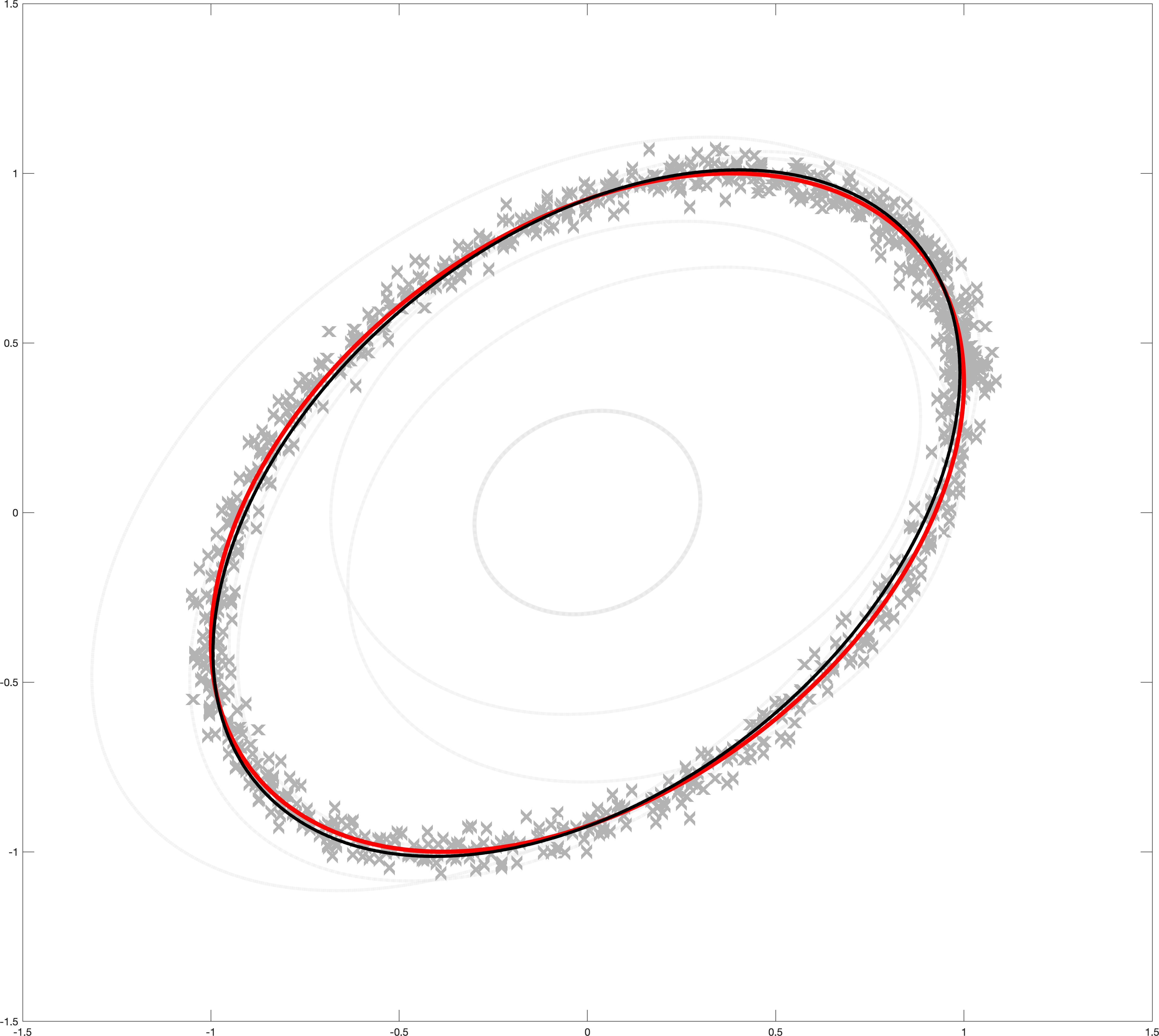
Interferometry was recently made famous due to its use in Nobel award winning detection of gravitational waves in 2015 [1]. Two 4km interferometers form the Laser Interferometer Gravitational-Wave Observatory, called LIGO for short. The measured intensity of each laser beam at time , denoted here as and , can be plotted against one another to reveal an elliptical shape as illustrated in Figure 4. This shape is essential to detecting reflector perturbations, but is typically not known. The aim is to estimate this ellipse based on observed data. We can parametrize this relationship as
| (66a) | ||||
| (66b) | ||||
where and denotes the position of the laser reflector, which is not directly measured. A suitable model for the dynamics is provided by a simple discrete-time kinematic relationship
| (67) |
where is the sample interval and is an unknown action on the system. The unknown parameters are collected as and the resulting maximum likelihood system identification problem can be expressed as (60). This problem construction is known as a blind Wiener problem [51]. We generated samples of the outputs using the above model with true parameter values indicated in Table 2. To calculate the likelihood and its gradient, we employed a particle filter with particles. A Monte-Carlo simulation with 100 runs was performed and the results are provided in Table 2. Figure 4 also provides the measured outputs for one simulation and plots the ellipse as the algorithm progresses. The final ellipse is indicated in solid black while the true ellipse is shown in red. Based on these results, it appears that Algorithm 2 appears to be performing quite well .
| QNGP Estimate | ||
|---|---|---|
7.4 MIMO Hammerstein-Wiener system
As a further example, we turn attention to the multiple-input/multiple-output (MIMO) Hammerstein-Wiener system from [51] (Section 6.2 in that paper). The system has two inputs, two outputs and 4’th order linear dynamics with saturation and deadzone static nonlinearities on the input and output channels. Full details of this system and the associated parametrization can be obtained from [51] and are not repeated here due to page limitations.
For the purposes of estimation, samples of the inputs and outputs were simulated. In this case, two different algorithms are compared:
- 1.
The SMC based Expectation-Maximisation method developed in [51], called the PSEM (particle smoother EM) approach;
- 2.
The quasi-Newton GP based solution presented in the current paper, denoted as QNGP.
For QNGP method, particles were used, and for QNGP particles were used (note that the computational complexity of the former method scales as , while the second SMC approach scales as , making the two comparable). The algorithms were terminated after iterations. The results of Monte Carlo runs for all algorithms are shown in Figures 5(a)–7. For each run, different noise realisations were used according to the distributions specified above. In each plot, the solid blue line indicates the true response, while the red lines indicate the mean (think dashed) and one standard deviation from mean (thin dashed).
This example shows that the proposed Algorithm 2 compares well to state-of-the-art methods such as PSEM. A potential benefit of the QNGP approach is that only forward filtering is required, whereas PSEM requires a SMC-based smoother, which can be challenging in general[26, 22].
8 Conclusion and future work
In this paper we have presented a new quasi-Newton algorithm for stochastic optimisation problems. The approach uses a tailored Gaussian process to model the unknown Hessian, which is then learned from gradient information as the algorithm progresses. To regulate the iterates, we developed a stochastic line-search procedure that satisfies an Armijo condition (in expectation) for early iterations, and converges to a deterministic step-length schedule as the iterations grow. The former provides a mechanism to handle poorly scaled problems while the Hessian is learned, and the latter mimics conditions required for convergence in the stochastic setting. The resulting combination is demonstrated on several challenging nonlinear system identification problems, with promising results. The method can be straightforwardly extended to handle the situation where—possibly noisy—Hessian matrices are also observed.
The GP construction assumes that the gradient is corrupted by additive Gaussian noise, and this is potentially not suitable for certain problem classes, particularly where the noise distribution has heavy tails. This allows for an extension to other processes such as the student-t process [46]. A further extension is for the case of large-scale problems, which frequently occur within the Machine Learning field. Some initial work in this direction can be found in [50].
Acknowledgements
This research is financially supported by the Swedish Research Council via the projects NewLEADS - New Directions in Learning Dynamical Systems (contract number: 621-2016-06079) and Learning flexible models for nonlinear dynamics (contract number: 2017-03807), and the Swedish Foundation for Strategic Research (SSF) via the project ASSEMBLE (contract number: RIT15-0012).
References
- [1] Benjamin P Abbott, Richard Abbott, TD Abbott, MR Abernathy, Fausto Acernese, Kendall Ackley, Carl Adams, Thomas Adams, Paolo Addesso, RX Adhikari, et al. Observation of gravitational waves from a binary black hole merger. Physical review letters, 116(6):061102, 2016.
- [2] L. Armijo. Minimization of functions having Lipschitz continuous first partial derivatives. Pacific Journal of Mathematics, 16(1):1–3, 1966.
- [3] H. Asi and J. C. Duchi. Stochastic (approximate) proximal point methods: convergence, optimality, and adaptivity. SIAM Journal on Optimization, To appear, 2019.
- [4] Dimitri P Bertsekas and John N Tsitsiklis. Neuro-dynamic programming, volume 5. Athena Scientific Belmont, MA, 1996.
- [5] R. Bollapragada, D. Mudigere, J. Nocedal, H.-J. M. Shi, and P. T. P. Tang. A progressive batching L-BFGS method for machine learning. In Proceedings of the 35th International Conference on Machine Learning (ICML), Stockholm, Sweden, 2018.
- [6] A. Bordes, L. Bottou, and P. Gallinari. SGD-QN: Careful quasi-Newton stochastic gradient descent. Journal of Machine Learning Research (JMLR), 10:1737–1754, 2009.
- [7] L. Bottou, F. E. Curtis, and J. Nocedal. Optimization methods for large-scale machine learning. SIAM Review, 60(2):223–311, 2018.
- [8] C. G. Broyden. A class of methods for solving nonlinear simultaneous equations. Mathematics of Computation, 19(92):577–593, 1965.
- [9] C. G. Broyden. Quasi-Newton methods and their application to function minimization. Mathematics of Computation, 21:368–381, 1967.
- [10] C. G. Broyden. The convergence of a class of double-rank minimization algorithms. Journal of the Institute of Mathematics and Its Applications, 6(1):76–90, 1970.
- [11] P. Del Moral. Feynman-Kac formulae: Genealogical and Interacting Particle Systems with Applications. Springer, New York, USA, 2004.
- [12] J. Duchi, E. Hazan, and Y. Singer. Adaptive subgradient methods for online learning and stochastic optimization. Journal of Machine Learning Research (JMLR), 12:2121–2159, 2011.
- [13] R. Fletcher. A new approach to variable metric algorithms. The computer journal, 13(3):317–322, 1970.
- [14] R. Fletcher. Practical methods of optimization. John Wiley & Sons, Chichester, UK, second edition, 1987.
- [15] R. Fletcher and M. J. D. Powell. A rapidly convergent descent method for minimization. The computer journal, 6(2):163–168, 1963.
- [16] D. Goldfarb. A family of variable metric updates derived by variational means. Mathematics of Computation, 24(109):23–26, 1970.
- [17] Graham C Goodwin, Peter J Ramadge, and Peter E Caines. Discrete time stochastic adaptive control. SIAM Journal on Control and Optimization, 19(6):829–853, 1981.
- [18] N. J. Gordon, D. J. Salmond, and A. F. M. Smith. Novel approach to nonlinear/non-Gaussian Bayesian state estimation. In IEE Proceedings on Radar and Signal Processing, volume 140, pages 107–113, 1993.
- [19] J. N. Hendriks, C. Jidling, A. Wills, and T. B. Schön. Evaluating the squared-exponential covariance function in Gaussian processes with integral observations. Technical report, arXiv:1812.07319, 2018.
- [20] P. Hennig. Probabilistic interpretation of linear solvers. SIAM Journal on Optimization, 25(1):234–260, 2015.
- [21] P. Hennig and M. Kiefel. Quasi-Newton methods: a new direction. Journal of Machine Learning Research (JMLR), 14:843–865, 2013.
- [22] N. Kantas, A. Doucet, S. S. Singh, J. M. Maciejowski, and N. Chopin. On particle methods for parameter estimation in state-space models. Statistical Science, 30(3):328–351, 2015.
- [23] Jack Kiefer and Jacob Wolfowitz. Stochastic estimation of the maximum of a regression function. The Annals of Mathematical Statistics, 23(3):462–466, 1952.
- [24] D. P. Kingma and J. Ba. Adam: a method for stochastic optimization. In Proceedings of the 3rd international conference on learning representations (ICLR), San Diego, CA, USA, 2015.
- [25] G. Kitagawa. A Monte Carlo filtering and smoothing method for non-Gaussian nonlinear state space models. In Proceedings of the 2nd US-Japan joint Seminar on Statistical Time Series Analysis, pages 110–131, 1993.
- [26] F. Lindsten and T. B. Schön. Backward simulation methods for Monte Carlo statistical inference. Foundations and Trends in Machine Learning, 6(1):1–143, 2013.
- [27] L. Ljung. Asymptotic behavior of the extended Kalman filter as a parameter estimator for linear systems. IEEE Transactions on Automatic Control, AC–24(1):36–50, February 1979.
- [28] L. Ljung and T. Söderström. Theory and Practice of Recursive Identification. The MIT Press series in Signal Processing, Optimization, and Control. The MIT Press, Cambridge, Massachusetts, 1983.
- [29] Lennart Ljung. Analysis of recursive stochastic algorithms. IEEE transactions on automatic control, 22(4):551–575, 1977.
- [30] Lennart Ljung. Strong convergence of a stochastic approximation algorithm. The Annals of Statistics, pages 680–696, 1978.
- [31] Lennart Ljung, Georg Pflug, and Harro Walk. Stochastic approximation and optimization of random systems, volume 17. Birkhäuser, 2012.
- [32] Liangchen Luo, Yuanhao Xiong, and Yan Liu. Adaptive gradient methods with dynamic bound of learning rate. In International Conference on Learning Representations (ICLR), New Orleans, LA, USA, 2019.
- [33] J. R. Magnus and H. Neudecker. The elimination matrix: some lemmas and applications. SIAM Journal on Algebraic Discrete Methods, 1(4):422–449, 1980.
- [34] M. Mahsereci and P. Hennig. Probabilistic line searches for stochastic optimization. Journal of Machine Learning Research (JMLR), 18(119):1–59, 2017.
- [35] S. Malik and M. K. Pitt. Particle filters for continuous likelihood evaluation and maximisation. Journal of Econometrics, 165(2):190–209, 2011.
- [36] A. Mokhtari and A. Ribeiro. RES: regularized stochastic BFGS algorithm. IEEE Transactions on Signal Processing, 62(23):6089–6104, 2014.
- [37] E. Moulines and F. Bach. Non-asymptotic analysis of stochastic approximation algorithms for machine learning. In Advances in Neural Information Processing Systems (NIPS), Granada, Spain, 2011.
- [38] J. Nocedal and S. J. Wright. Numerical Optimization. Springer Series in Operations Research. Springer, New York, USA, second edition, 2006.
- [39] M. K. Pitt, R. dos Santos Silva, R. Giordani, and R. Kohn. On some properties of Markov chain Monte Carlo simulation methods based on the particle filter. Journal of Econometrics, 171(2):134–151, 2012.
- [40] G. Poyiadjis, A. Doucet, and S.S. Singh. Particle approximations of the score and observed information matrix in state space models with application to parameter estimation. Biometrika, 98(1):65–80, 2011.
- [41] C. E. Rasmussen and C. K. I. Williams. Gaussian processes for machine learning. MIT Press, 2006.
- [42] H. Robbins and S. Monro. A stochastic approximation method. Annals of Mathematical Statistics, 22(3):400–407, 1951.
- [43] T. B. Schön, F. Lindsten, J. Dahlin, J. Wågberg, A. C. Naesseth, A. Svensson, and L. Dai. Sequential Monte Carlo methods for system identification. In Proceedings of the 17th IFAC Symposium on System Identification (SYSID), Beijing, China, October 2015.
- [44] T. B. Schön, A. Wills, and B. Ninness. System identification of nonlinear state-space models. Automatica, 47(1):39–49, January 2011.
- [45] N. N. Schraudolph, J. Yu, and S. Günter. A stochastic quasi-Newton method for online convex optimization. In Proceedings of the 11th international conference on Artificial Intelligence and Statistics (AISTATS), 2007.
- [46] A. Shah, A. G. Wilson, and Z. Ghahramani. Student-t processs as alternatives to Gaussian processes. In Proceedings of the 17th international conference on artificial intelligence and statistics (AISTATS), Reykjavik, Iceland, May 2014.
- [47] D. F. Shanno. Conditioning of quasi-Newton methods for function minimization. Mathematics of Computation, 24(111):647–656, 1970.
- [48] James C Spall. Introduction to stochastic search and optimization: estimation, simulation, and control, volume 65. John Wiley & Sons, 2005.
- [49] L. Stewart and P. McCarty. The use of Bayesian belief networks to fuse continuous and discrete information for target recognition and discrete information for target recognition, tracking, and situation assessment. In Proceedings of SPIE Signal Processing, Sensor Fusion and Target Recognition, volume 1699, pages 177–185, 1992.
- [50] A. Wills and T. B. Schön. Stochastic quasi-Newton with adaptive step lengths for large-scale problems. arXiv:1802.04310, 2018.
- [51] A. Wills, T. B. Schön, L. Ljung, and B. Ninness. Identification of Hammerstein-Wiener models. Automatica, 49(1):70–81, 2013.
- [52] A. G. Wills and T. B. Schön. On the construction of probabilistic Newton-type algorithms. In Proceedings of the 56th IEEE Conference on Decision and Control (CDC), Melbourne, Australia, December 2017.
- [53] P. Wolfe. Convergence conditions for ascent methods. SIAM Review, 11(2):226–235, 1969.
- [54] P. Wolfe. Convergence conditions for ascent methods II: some corrections. SIAM Review, 13(2):185–188, 1971.
Appendix A The stochastic Armijo condition
All expectation below are conditioned on the variables . This conditioning is dropped from the notation in order to improve readability. The required expectation is
| (68) |
and recall that
| (69a) | ||||
| (69b) | ||||
| (69c) | ||||
| (69d) | ||||
Assume that and . Since is assumed twice continuously differentiable on , then employing Taylor’s theorem results in
| (70) |
for some . Hence, using (1) and (70) then (68) becomes
which reduces to
Let and , then division on both sides by results in
| (71) |
where . Since both and then , and . Therefore, for small enough, then (71) is satisfied for