Magnetorotational core collapse of possible GRB progenitors. I. Explosion mechanisms.
Abstract
We investigate the explosion of stars with zero-age main-sequence masses between 20 and 35 and varying degrees of rotation and magnetic fields including ones commonly considered progenitors of gamma-ray bursts (GRBs). The simulations, combining special relativistic magnetohydrodynamics, a general relativistic approximate gravitational potential, and two-moment neutrino transport, demonstrate the viability of different scenarios for the post-bounce evolution. Having formed a highly massive proto-neutron star (PNS), several models launch successful explosions, either by the standard supernova mechanism based on neutrino heating and hydrodynamic instabilities or by magnetorotational processes. It is, however, quite common for the PNS to collapse to a black hole (BH) within a few seconds. Others might produce proto-magnetar-driven explosions. We explore several ways to describe the different explosion mechanisms. The competition between the timescales for advection of gas through the gain layer and heating by neutrinos provides an approximate explanation for models with insignificant magnetic fields. The fidelity of this explosion criterion in the case of rapid rotation can be improved by accounting for the strong deviations from spherical symmetry and mixing between pole and equator. We furthermore study an alternative description including the ram pressure of the gas falling through the shock. Magnetically driven explosions tend to arise from a strongly magnetised region around the polar axis. In these cases, the onset of the explosion corresponds to the equality between the advection timescale and the timescale for the propagation of Alfvén waves through the gain layer.
Keywords:
Supernovae: general - gamma-ray bursts: general1 Introduction
The collapse of the core of a massive star of more than about 8 solar masses at the end of its hydrostatic evolution is the starting point for a complex sequence of events with many possible outcomes (Janka et al. 2016; Müller 2016, for reviews, see, e.g.,). The post-collapse evolution depends strongly on factors such as the mass and metallicity of the progenitor, its rotation and magnetic field, and potentially on the individual realization of stochastic processes such as hydrodynamic instabilities. During the subsequent period of up to several seconds, neutrinos streaming out of the proto neutron star (PNS) transfer energy to the gas behind the stalled shock wave and, together with hydrodynamic instabilities, and possibly other effects such as rotation and magnetic fields, favour shock revival. For a successful core-collapse supernova (CCSN) explosion to occur, they have to unbind at least parts of the matter surrounding the PNS and overcome the continuous infall of matter at high velocities towards the PNS. The properties of the explosion such as mass, composition, velocity, energy, and geometry of the ejecta depend strongly on the progenitor and on the relative importance of different processes contributing to shock revival. This view is corroborated by observations of a wide variety of CCSNe ranging from low-luminosity events to very energetic ones characterized by high expansion velocities and pronounced global asymmetries (Woosley & Bloom 2006; Cano et al. 2017; Moriya et al. 2018, see, e.g.).
We are interested in the core collapse of stars in a regime where all of the aforementioned evolutionary paths overlap. The goal is to study the physics of explosions of rapidly rotating stars at different metallicities, with different magnetic fields and initial masses and to explore the conditions for the development of long GRB engines. More specifically, we focus on the following issues:
- 1.
Do stars commonly considered likely long GRB progenitors explode in CCSNe?
- 2.
If so, what mechanism produces the shock revival and what are the characteristics of the explosion?
We aim to model stars likely to produce high-mass PNSs while at the same time close to the threshold between successful explosion and failed shock revival. Based on the aforementioned considerations, we select several stars of and (Woosley et al. 2002; Woosley & Heger 2006; Woosley & Heger 2007) that, while differing in their metallicity, and, in case of stars that were evolved including the effects of rotation and magnetic fields, also the mass loss rates, are all close to the explosion threshold.
Our progenitors differ by their mass, structure, rotation and magnetic field from those studied most extensively in supernova theory. Consequently, we expect deviations from the standard scenario for explosions driven by neutrino heating that is aided by hydrodynamic instabilities (Janka 2012, for a review, see, e.g.). In particular, rotation and possibly magnetic fields are likely to contribute to the explosion mechanism. Rapid rotation may lead to global asymmetries of the shock wave, and of the neutrino emission, which translate into the formation of bipolar outflows (Obergaulinger & Aloy 2017). These effects are most pronounced when rotation is combined with a strong magnetic field that can tap into the rotational energy, as has been demonstrated in multi-dimensional simulations with varying degrees of approximations regarding the microphysics (Bisnovatyi-Kogan et al. 1976; Müller & Hillebrandt 1979; Symbalisty 1984; Akiyama et al. 2003; Kotake et al. 2004; Thompson et al. 2005; Moiseenko et al. 2006; Obergaulinger et al. 2006a; Obergaulinger et al. 2006b; Dessart et al. 2007; Burrows et al. 2007; Winteler et al. 2012; Sawai et al. 2013; Mösta et al. 2014; Mösta et al. 2015, see, e.g.). The dynamic relevance of the magnetic field depends crucially on the ratio of the magnetic energy to the kinetic energy, which in most, though not all, typical pre-collapse cores is expected to be rather small. Hence, processes that amplify the seed field such as flux-freezing compression, winding by the differential rotation, or dynamos driven by the MRI or hydrodynamic instabilities are important ingredients to the overall picture (Akiyama et al. 2003; Obergaulinger et al. 2009; Masada et al. 2012; Mösta et al. 2015; Guilet & Müller 2015; Masada et al. 2015; Rembiasz et al. 2016b; Rembiasz et al. 2016a; Sawai & Yamada 2016; Guilet et al. 2017). Explosions partially modified or predominantly driven by these processes have been invoked to explain several very energetic and aspherical events associated to hypernovae (Wheeler et al. 2002; Maeda & Nomoto 2003; Dessart et al. 2008; Tominaga 2009; Dessart et al. 2012; Mazzali et al. 2014; Wang et al. 2015; Tchekhovskoy & Giannios 2015; Metzger et al. 2015; Chen et al. 2016).
In order to undertake the previously mentioned point (ii), we compare the evolution across numerical simulations, where we vary the rotation profiles and the magnetic fields of our pre-collapse cores. Our simulations are based on a state-of-the-art code combining high-order methods for solving the hyperbolic terms of the MHD and transport equations with a post-Newtonian treatment of gravity, as well as a spectral two-moment neutrino transport including corrections due to the velocity (Doppler shifts, aberration) and the gravitation field (gravitational blue/redshift) and the relevant reactions between neutrinos and matter. The rather long simulation times we want to reach (various seconds post-bounce) and the variety of models we need to explore limit us to consider only two low-resolution three-dimensional (3D) models, which are prototypes of collapsar- and PM-forming central engines. These cases present qualitatively the same behaviour in 3D than in 2D. Encouraged by the similarity of the results, but aware of the fact that the final answers can only come from unrestricted 3D models, we explore many other cases employing axisymmetric models.
2 Physics and numerics
The simulations were performed using the neutrino-MHD code presented in Just et al. 2015. With respect to the description of the algorithms, implementation, and tests given there (Rembiasz et al. 2017, and in) and to the previous application in simulations of magnetized core collapse (Obergaulinger et al. 2014), we have made several modifications for the purpose of running the present set of models. These modifications have already been used in closely related publications (Obergaulinger & Aloy 2017; Aloy & Obergaulinger 2019, Paper II hereafter), as well as in the exploration of magneto-rotational collapse of lower mass and solar metallicity progenitors (Obergaulinger et al. 2018). Below we detail all these modifications for the sake of completness.
The MHD system and the hyperbolic part of neutrino transport are solved in a finite-volume discretization in spherical coordinates, , assuming axisymmetry. We employ the constrained-transport method for avoiding a non-zero divergence of the magnetic field (Londrillo & del Zanna 2004) and use high-resolution shock-capturing methods combining high-order reconstruction (Suresh & Huynh 1997, the monotonicity-preserving method of order (MP5) of) and approximate Riemann solvers (for MHD, HLLC, see Mignone & Bodo 2006, for the neutrinos, HLL). We employ an explicit -order Runge-Kutta time integrator for all terms but the stiff source terms, which our code integrates implicitly (Just et al. 2015, for the implementation, see).
In the following, we will use natural units, where both the speed of light in vacuum, , and the gravitational constant are taken to be . Furthermore, roman indices , and run along the three spatial dimensions, , while annotates the species number.
2.1 Special relativistic MHD
Here, in contrast to our earlier work based on Newtonian MHD, we solve the equations of special relativistic MHD, i.e. the conservation laws for relativistic mass density, , partial densities of charged particles (electrons and protons), , and of a set of chemical elements, , relativistic momentum and energy density, and , respectively, and magnetic field, ,11 1 We express all 3-vectors in orthonormal bases, so that covariant and contravariant components are interchangeable.
| (1) | |||||
| (2) | |||||
| (3) | |||||
| (4) | |||||
| (5) | |||||
| (6) | |||||
| (7) |
The operator () contains the determinant of the spatial metric, , which does not depend on time. The fluxes are functions of the primitive variables: velocity, , and Lorentz factor, , rest-mass density, , electron fraction, , and gas pressure, .
The relations between conserved and primitive variables are
| (8) | |||||
| (9) | |||||
| (10) |
where () is the square of the magnetic field four vector, whose temporal and spatial components are, respectively
| (11) | |||||
| (12) |
For recovering the primitive variables, we use the same techniques as in Leismann et al. 2005 or Cerdá-Durán et al. 2008.
Since the relations inverting Eqs. (8)-(10) are not explicit, the momentum and energy fluxes are given in terms of a combination of conserved and primitive variables:
| (13) | |||||
| (14) |
with being the Kroneker delta. The other quantities appearing in the MHD equations are the lapse function, , and the source terms accounting for the exchange of lepton number, momentum, and energy between matter and neutrinos, , and , respectively. The source terms denoted with the subscript are the integrals over neutrino energy, summed over all neutrino flavours of the spectral neutrino-matter interaction terms, which we will discuss below.
In the stars with , the gas pressure is determined by the equation of state (EOS) of Lattimer & Swesty 1991 with a nuclear incompressibility of (LS220 hereafter) for densities above . At lower densities, we use an EOS containing contributions of electrons and positrons, photons, and baryons and the flashing scheme of Rampp & Janka 2002. The general way in which this scheme changes the nuclear composition of the gas is represented by the set of source terms . We employ the same low-density EOS in the models with , but a different high-density EOS, viz. SFHo of Steiner et al. 2013. Because, this EOS is tabulated for a wider range of densities, we switch between it and the low-density EOS at a lower density of . We note that the maximum baryonic mass (in the non-rotating and zero temperature limit) is for both EoSs (LS220 and SFHo).
We compute the gravitational potential, , according to version ’A’ of the post-Newtonian TOV potentials of Marek et al. 2006. To ensure consistency with the gravitational terms in the equations of neutrino transport (see below), we include the lapse in the spatial derivatives. Since we do not model gravity by a general relativistic 3+1 metric, we define the lapse function based on the classical gravitational potential, , as .
2.2 Neutrino transport
We treat the neutrino transport in the two-moment framework closed by the maximum-entropy Eddington factor (Cernohorsky & Bludman 1994). As in Obergaulinger & Aloy 2017 and Obergaulinger et al. 2018, we include the effects of gravity in the neutrino-transport equations in the -plus formulation of Endeve et al. 2012:
| (15) | |||||
| (16) | |||||
where and are the second and third moment of the neutrino distribution function, respectively, and is the acceleration. The momentum equation involves the third moment, for which we use the approximation given in Just et al. 2015. The terms involving that appear in addition to the ones contained in our earlier work are implemented in an analogous fashion to the formally very similar expressions in the velocity-dependent terms see (Just et al. 2015, for details, see).
2.3 Neutrino-matter interaction
The most important change with respect to the basic set of reactions from Obergaulinger et al. 2014 consists in the addition of pair processes, electron-positron annihilation and nucleonic bremsstrahlung, in the implementation of which we follow Pons et al. 1998 and Hannestad & Raffelt 1998, respectively. Hence, neutrinos of all flavours are produced in our simulations (Obergaulinger et al. 2014, in contrast to the ones of). The other reactions included are: (i) nucleonic absorption, emission, and scattering with the corrections due to weak magnetism and recoil; (ii) nuclear absorption, emission, and scattering; (iii) inelastic scattering off electrons.
3 Initial models and parameters
| star | ||||||
|---|---|---|---|---|---|---|
| 35OC | 28.1 | 2.4 | 2.0 | 3.0 | 2.0 | 0.1 |
| 35OB | 21.2 | 3.2 | 2.2 | 2.8 | 1.5 | 0.05 |
| s20 | 14.7 | 5.8 | 1.5 | 1.7 | ||
| z35 | 35.0 | 2.2 | 2.3 | 3.2 |
As we focus in particular on the effects of rotation and magnetic fields, it should be pointed out that all progenitor models are the result of spherically symmetric stellar evolution calculations. Some of them (models 35OB/C, see below) include approximate prescriptions for rotational dynamos and the feedback of the magnetic field on the stellar structure, whereas others do not incorporate them at all. In the former case, we could base the pre-collapse distributions of angular velocity and magnetic field on the stellar-evolution models. For the latter class of models, we add different distributions of the angular velocity and the magnetic field to the spherically symmetric pre-collapse stellar configurations. For the sake of comparison, we employ the same technique for additional simulations of the former models. We finally note that some of the simulations have been presented already (Obergaulinger & Aloy 2017; Obergaulinger et al. 2018), but some of the models have been evolved further in time. Here, we present a more comprehensive investigation of the processes that lead to a successful explosion or lack thereof.
We use the progenitor model 35OC, which was computed by Woosley & Heger 2006 as a model for a rapidly rotating star of zero-age main-sequence mass including the redistribution of angular momentum by magnetic fields according to the theoretical framework of Spruit 2002. We used another model from the same series of progenitors, model 35OB, which was constructed assuming a stronger mass loss than model 35OC, leading to a lower pre-collapse mass and a slower rotating iron core. The group of pre-collapse models computed without rotation and magnetic fields consists of two progenitors with solar metallicity and (Woosley & Heger 2007, model s20) and one with zero metallicity and (Woosley et al. 2002, model z35). The properties of these four stars are summarised in Tab. 1.
We map the pre-collapse structure of the core (computed in one spatial dimension), viz. the hydrodynamic variables such as density, electron fraction, temperature, and rotational velocity, onto our simulation grid. The magnetic field of the model is the result of MHD instabilities. Hence, it is not a global, e.g. dipole field encompassing the entire star, but rather confined to several shells. It is given in terms of the absolute values of the toroidal and a poloidal component as functions of radius only. Because we lack detailed information on the orientation of the field vectors as well as the angular distribution of the field strength, we treat the magnetic field as an additional parameter of our models. We simulate a series of models based on the field as given by the pre-collapse model and an additional series of models in which we replace the field by a global dipole field and a toroidal component. Assessing the impact of multipolar magnetic topologies on the post-collapse outcome is beyond the scope of this paper, but we refer interested readers to the detailled study of Bugli et al. 2019. In the former series of models, we set the -component of the initial field proportional to the toroidal component of the stellar-evolution model,
| (17) |
and compute the -component from its poloidal component
| (18) |
where and are dimensionless parameters. The -component follows directly from the solenoidal condition. In the latter series of models, in which we lack of magnetic fields in the progenitor or we replace the stellar evolution field by a large-scale magnetic dipole, we compute the poloidal components from a vector potential, (Suwa et al. 2007, e.g.). The -component of is given in terms of two parameters, and ,
| (19) |
and add a toroidal component proportional to ,
| (20) |
Within each of the two series, we vary the normalization of the poloidal and toroidal components, and, in the first series, also their angular distribution. In order to assess the importance of rotation, we add a version of the same model with an artificially modified (either reduced or increased) angular velocity.
All models were simulated on spherical grids. In the case of axially symmetric models, the mesh consisted of zones in -direction and radial zones with a width given in terms of a parameter
| (21) |
Compared to other simulations in the literature, the central grid spacing is relatively coarse, but it is comparable with the values m used by, e.g. Dimmelmeier et al. 2002. We do, however, not see any of the commonly observed artefacts of an insufficient radial resolution such as a possible expansion of the PNS surface. We attribute this fact to our use of high-order reconstruction schemes, which, as shown by Rembiasz et al. 2017 greatly reduce the numerical errors w.r.t. lower-order schemes. For an assessment of the behaviour of this code and its dependence on different assumptions and approximations for the neutrino physics as well as on the grid resolution, see Just_et_al__2018__ArXive-prints__Core-collapsesupernovasimulationsinoneandtwodimensions:comparisonofcodesandapproximations.
As a result of the setup expressed by Eq. 21, the grid width is uniform inside a certain radius and increases outside of this radius linearly with in such a manner that the zones have an aspect ratio very close to unity. In addition, we apply a coarsening scheme close to the origin in order to increase the time step allowed by the CFL condition and to obtain effective zones of aspect ratio , there, too. To save computing time, we simulated the collapse of the models (during which angular resolution is not crucial) in axisymmetry in lower resolution (the same radial grid, but ) and mapped to the standard grid shortly before bounce.
In energy space, we used energy bins distributed logarithmically between and . This may seem a rather low resolution, but we made sure by several series of spherically symmetric tests that our choice does not affect the results.
The models and their most important properties described in the following are introduced in Tab. 2.
| name | star | rotation | field | fate | BH |
| 35OC-RO | 35OC | Or | Or | MR | |
| 35OC-RO2 | 35OC | Or | MR | ||
| 35OC-Rp2 | 35OC | Or | MR | ||
| 35OC-Rp3 | 35OC | Or | MR | ||
| 35OC-Rp4 | 35OC | Or | MR | ||
| 35OC-Rw | 35OC | Or | - | ? | |
| 35OC-Rs | 35OC | Or | MR | ||
| 35OC-Sw | 35OC | ||||
| 35OC-RRw | 35OC | Or | - | ||
| 35OC-RO-TOV | 35OC | Or | Or | MR | |
| 35OB-RO | 35OB | Or | Or | - | |
| 35OB-RRw | 35OB | Or | |||
| s20-1 | s20 | R | a(10,11) | ||
| s20-2 | s20 | a(0.1) | a(10,11) | ||
| s20-3 | s20 | a(1.0) | a(11,11) | MR | |
| s20-2noB | s20 | a(0.1) | 0 | ||
| s20-3noB | s20 | a(1.0) | 0 | ||
| z35-Sw | z35.0 | a(0.5) | a(8,10) | ||
| z35-Rw | z35.0 | a(1.0) | a(8,10) | - |
4 Results
In the following, we will present a general outline of the dynamics of the models, characterising them according to the aforementioned evolutionary paths (Sect. 4.1). This presentation will be followed by a deeper look at several effects that shape the evolution of the cores (Sect. 4.2). We conclude this section with an analysis of the results in the light of a few conditions that have been suggested for shock revival (Sect. 4.3).
4.1 Overview
| Model | ||||||||||||||||||||||||
|---|---|---|---|---|---|---|---|---|---|---|---|---|---|---|---|---|---|---|---|---|---|---|---|---|
| s20-2 | ||||||||||||||||||||||||
| s20-3 | ||||||||||||||||||||||||
| 35OC-RO | ||||||||||||||||||||||||
| 35OC-RO2 | ||||||||||||||||||||||||
| 35OC-Rp2 | ||||||||||||||||||||||||
| 35OC-Rp3 | ||||||||||||||||||||||||
| 35OC-Rp4 | ||||||||||||||||||||||||
| 35OC-RRw | ||||||||||||||||||||||||
| 35OC-Rs | ||||||||||||||||||||||||
| 35OC-Rw | ||||||||||||||||||||||||
| 35OC-Sw | ||||||||||||||||||||||||
| 35OB-RO | ||||||||||||||||||||||||
| 35OB-RRw | ||||||||||||||||||||||||
| z35-Rw | ||||||||||||||||||||||||
| z35-Sw | ||||||||||||||||||||||||
Owing to their wide range of progenitor conditions, we find among our models very distinct evolutionary paths. Where they fall in this characterisation is summarised in Tab. 2. The path of a given model is not a function of the progenitor mass only, but is crucially affected by the detailed structure, in particular the compactness of the core (O’Connor & Ott 2011, see), its rotational energy, and its magnetisation (Obergaulinger & Aloy 2017). Varying only the rotational profile or only the magnetic field strength can completely change the evolution of a core. Of course, it should be noted that while a variation of only one property of a stellar model is possible in the idealised setting of a numerical study, it would in reality entail a major adaption of all aspects of the structure of the star. Hence, some of our modifications are a bit artificial and, thus, should not be treated as predictions for the evolution of a particular star of a given mass and rotational and magnetic energy but rather as a parameter study to tackle the impact of individual processes. Besides, the progenitors we employ are the result of one-dimensional stellar evolution models, which incorporate rotation and the dynamical effects of magnetic fields with a limited accuracy. In most cases, these models employ parameterizations of key effects such as mass-loss or the braking action of magnetic fields. Relatively small variations in these parameters result in changes of the pre-collapse magnetic field and angular velocity distribution, which we attempt to mimic with our parametrized variations of these structural properties.
We show an overview of some of the most important global quantities characterising the evolution of the models (PNS mass, maximum shock radius, diagnostic explosion energy, ejecta mass) in Figs. 1–3. Furthermore, Tab. 3 summarises properties of the models at the point of explosion.
4.1.1 Neutrino-driven explosions
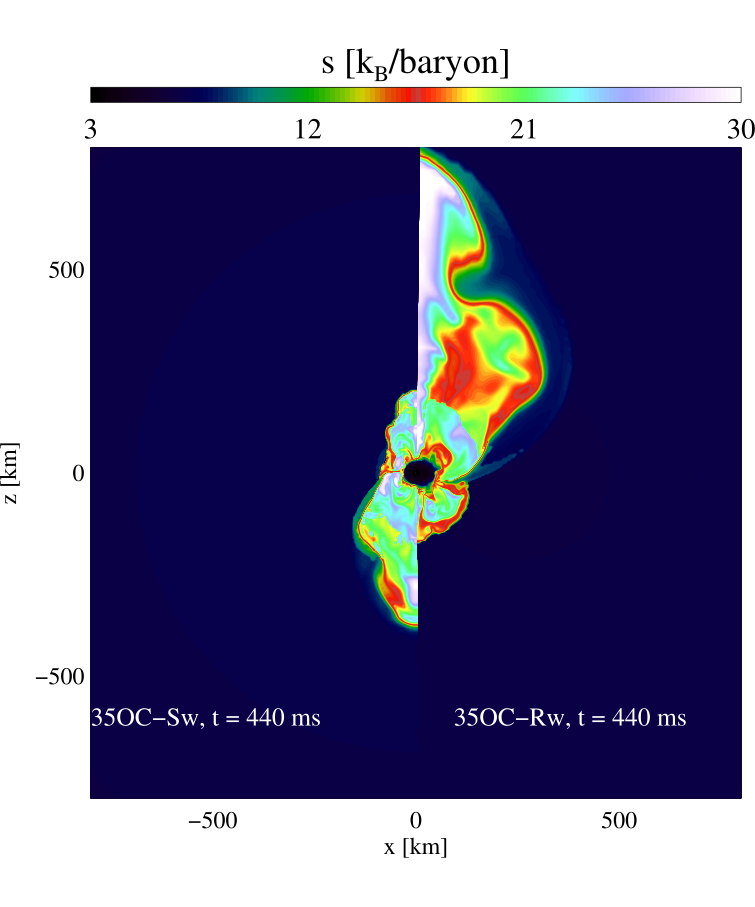
Some of our models achieve shock revival by neutrino heating aided by non-spherical gas flows. In some of them, rotation causes important modifications w.r.t. to the standard scenario for SN. Examples for the first (purely neutrino driven) and second (neutrino-rotationally driven) scenario are models 35OC-Sw and 35OC-Rw, respectively.
Most models launch an explosion within a few hundred milliseconds post-bounce after a phase of pronounced activity of hydrodynamic instabilities in the gain layer (Tab. 3). Based on the predominance of structures of angular extents of several tens of degrees in the post-shock flow as well as in the deformations of the shock surface, we characterise the models as dominated by convection rather than by the standing accretion shock instability (SASI). Magnetic fields are amplified in the gain layer and in the PNS, but do not grow sufficiently as to affect the shock revival. For both moderately and rapidly rotating models, the supernova shock wave starts to expand at high latitudes and the explosions take the form of wide uni- or bipolar outflows along the symmetry axis (Fig. 4), into which a fraction of the matter falling onto the PNS is redirected, mostly through downflows at low latitudes. The precise geometry of the downflows as well as the angular width of the outflows and their fluxes of energy and mass can fluctuate strongly with time.
Models of this class display a wide range of (diagnostic) explosion energies and ejecta masses. Most have energies a bit less than the canonical SN explosion of , but a few (models 35OC-Sw and 35OC-Rw; see Fig. 2) exceed that value by the end of the simulation and the growth of the energy indicates that others (e.g. models s20-2, Fig. 1, and 35OB-RO, Fig. 3) are likely to do so shortly after the end of the simulations.
We note that a successful explosion and the formation of a BH are not mutually exclusive. Downflows increasing the PNS mass may coexist with gas ejected in a very asymmetric manner. Hence, we encounter BH formation among exploding models such as model 35OC-Sw. A discussion of the possible connection of such a scenario to the engines of long GRBs within the collapsar model as well as the activity of proto-magnetars as an alternative route to GRBs is performed in a companion study (Paper II).
Finally, although successful explosions are the most common outcome, several models, e.g. model s20-1/2noB/3noB, fail to achieve shock revival within the simulation time. The failure, if definite, will ultimately lead to the collapse of the PNS to a BH, similar to the findings of Pan et al. 2018; Chan et al. 201822 2 We note that the final collapse of the PNS to a BH may be affected by the choice of EOS (Aloy et al. 2019, see). In a few cases, we could follow the evolution long enough to reach this point, while in others the PNS mass grows too slowly for collapse to occur within the simulation time of up to more than 2 seconds. As the sequence of models with the progenitor s20 shows, shock revival may fail at slow as well as rapid rotation. In the latter case, the reduction of the accretion luminosity due to very deformed PNSs can be a decisive factor in avoiding an explosion.
The extremely rapidly rotating models 35OB-RRw and z35-Rw (see Fig. 3) constitute cases at the boundary between successful shock revival and failed explosions. Their very high rotational energy causes them to develop extremely oblate cores whose neutrinospheres extend to more than 100 km in the equatorial plane. As a consequence, the gas falling towards the centre settles down at comparably high radii, releasing less gravitational binding energy. The neutrino luminosity is, hence, smaller than in models with less flattened PNSs, which reduces the prospects of neutrino-driven shock revival. Their shock waves start to expand rather gradually at late times (more than a second after bounce) and the post-shock gas achieves comparably small positive energies around . Whether these energies are sufficient for the shock to reach the stellar surface after the potential collapse of the very massive PNSs to BHs is unclear, and would require much longer computational times to be assessed.
4.1.2 Magnetorotationally driven explosions
Various processes can amplify the seed magnetic field of the core such as compression by the radial flow, differential rotation, and hydromagnetic instabilities with the MRI potentially playing a very important role. We defer a detailed discussion of its development to a follow-up study focusing on the processes in the PNS and, for the current analysis, start with the observation that several models develop strong magnetic fields by a combination of the aforementioned effects.
A sufficiently strong magnetisation may lead to explosions driven by Maxwell stresses (with rotational contributions of different degree of importance), which can set in earlier than their essentially non-magnetic counterparts and may considerably exceed those in terms of the explosion energies, such as in models 35OC-Rs, 35OC-RO2, 35OC-Rp2, 35OC-Rp3, 35OC-Rp4, and 35OC-RO compared to the weaker magnetised version, 35OC-Rw. Also s20-3 belongs to this set of models.
Even more than for weakly magnetised models, bipolar explosion morphologies are characteristic for strongly magnetised ones. In particular the most intense magnetic fields are able to accelerate collimated jets with moderately relativistic flow speeds of up to . The explosions tend to be the more energetic the stronger the magnetic field is, with model 35OC-Rs as the most violent explosion reaching a diagnostic explosion energy of within less than one second. The strong explosions partially suppress the accretion of gas onto the PNSs, which therefore grow slower than for weaker magnetic fields. The suppression is most evident for models 35OC-Rs and 35OC-Rp4, where the PNS mass ceases to grow after (Fig. 2). Models 35OC-Rp2 and 35OC-Rp3 develop a local maximum at about the same time (), but then they grow again after s. In the case of model 35OC-Rp2 a second local maximum () is reached at s postbounce, while model 35OC-Rp3 displays an ongoing PNS mass growth by the end of the computed time (s). The behaviour of model 35OC-Rs after the maximum is explained in terms of the morphological changes that the PNS undergoes. It changes its shape from a prolate ellipsoid to a toroid at s (note the local minimum in the green line of the upper panel of Fig. 2). These two configurations display morphologies akin to the A and C types found by, e.g. Studzińska et al. 2016 for differentially rotating polytropes, respectively. Indeed our results suggest that transitions between different types of differentially rotating quasi-equilibrium models may be produced as a result of the accretion/ejection of mass onto/from the PNS outermost layers. Note that the strong decrease of the in model 35OC-Rs is possible as a combination of two facts. Firstly, the angular momentum redistribution resulting from the magnetic stress acting on this extremely magnetized initial configuration and, second, because these magnetic fields revert the accretion of mass onto the PNS, yielding a mass ejection (see the fast increase of the ejecta mass after the local maximum of is reached; Fig. 2).
4.2 Elements of the dynamics
In order to understand the dynamics, we will explore how various processes shaping their evolution differ across the range of initial models.
4.2.1 Mass accretion
We present the evolution of the total, i.e. angularly integrated, mass flux through the shock wave, , of all models in Fig. 5. The variations in this quantity reflect the structure of the progenitor star. The more or less sudden drops in correlate with the different shells of the progenitor star and the interfaces between them. A further decrease can be noted after the onset of an explosion as the shock wave propagates out into shells of lower density and encounters a reduced mass flux.
Our models exhibit the following values of after the accretion of the first stellar interface: for model s20-1, we find after , for model 35OC-Sw, between and the collapse to a BH, for model 35OB-RRw, after , and for model z35-Sw, after . Suwa et al. 2016 investigated the mass accretion history of an extended set of progenitors, compared to which our models show fairly high values. Their analysis, limited to models without magnetic fields, would suggest that rather high neutrino luminosities are required to trigger explosions in our models. A first conclusion from this comparison is that strong magnetic fields circumvent the condition on the neutrino luminosities as they are able to launch an explosion at mass accretion rates far exceeding those in which models with weak or vanishing fields undergo shock revival. The most prominent examples are model 35OC-Rs, and 35OC-RO2 exploding before the accretion of the surface of the -core at mass accretion rates around , but also models s20-3, and 35OC-RO start their explosions slightly before the strong decrease in the mass accretion rate. Compared to model s20-3, the slower rotation and weaker magnetic fields of model s20-2 seem to go into the same direction, enabling an explosion at a phase in which the other models of the same progenitor (models s20-1, s20-2noB, s20-3noB) fail to explode.
4.2.2 Neutrino emission
The time evolution of the total, i.e. angle-integrated, neutrino luminosities of our models, shown in the left panels of Fig. 6, correlates with the dynamics in several ways:
- 1.
After the neutrino burst emitted at bounce, all neutrino flavours maintain high luminosities whose precise values depend on the mass accretion rate. Models of progenitors s20 (top left panel) and 35OC (middle left panel), e.g. exhibit high luminosities until and , respectively. After that, the decreases of occurring when an interface between two shells falls onto the PNS correspond to notable decreases in the emission of neutrinos.
- 2.
The variation of the luminosities among models of a series with the same progenitor, but different rotation and magnetic field can be relatively minor as in the group of models corresponding to the s20 stellar progenitor or considerable as for model series 35OC. In the former case, the main factor distinguishing between the neutrino light curves is the beginning of an explosion, which leads, by virtue of the decreased mass accretion rate, to a lower neutrino emission. Among the models of group 35OC, on the other hand, the one with slowest rotation, 35OC-Sw, surpasses the neutrino luminosities of the rapid rotators with a delayed explosion (35OC-Rw and 35OC-RO) by about at . They in turn exceed the early exploding models 35OC-RO2 and 35OC-Rs by about the same factor. The inverse correlation between rotational velocity and neutrino emission is also observed for the other two groups of models.
We combine the two quantities discussed so far and display the evolution of the models in the phase space of mass accretion rate and combined electron neutrino and anti-neutrino luminosities in the right panels of Fig. 6 similarly to previous studies (Burrows & Goshy 1993; Murphy & Burrows 2008; Nordhaus et al. 2010; Fernández 2012; Hanke et al. 2012; Janka 2012; Suwa et al. 2016; Ertl et al. 2016). As in general the mass accretion rate decreases with time, the models traverse the diagrams from the right to the left. Their trajectories are represented by solid lines and symbols before and after the onset of an explosion, respectively. Hence, the point where a line ends marks the conditions at the revival of the shock wave (henceforth, revival luminosities and mass accretion rates). A relation between the mass accretion rate and a critical luminosity required for launching an explosion should show up in the distribution of the end points of the trajectories.
However, we do not find any evidence for any such direct relation. On the contrary, explosions seem to occur almost randomly across the entire space of parameters. Several models explode at moderate . Within this group, however, the revival luminosities differ significantly. We point, e.g. to models s20-2, 35OC-Sw, z35-Sw, and 35OB-RO with revival luminosities differing by a factor of about two Tab. 3. The connection between the --trajectories and the actual evolution of the models is complicated further by the fact that some models fail to explode at values of and that correspond to the shock revival in others. We refer to, e.g. models s20-1 and s20-2noB that, in contrast to model s20-2 with a very similar trajectory, do not explode when reaching values around and .
The consideration of strong magnetic fields further complicates finding a distinction between exploding and non-exploding models in this space of parameters. The early explosions of, e.g. models 35OC-Rs/O/O2 or s20-3 occurs at large . While the revival luminosities are large as well, they are exceeded by the values of non-exploding models at the same mass accretion rates.
To view the interplay of the two processes of accretion and heating by neutrinos from a different perspective, we consider the time scales for advection through the gain layer, , and heating, (Janka 2001; Thompson et al. 2005; Murphy & Burrows 2008, see, e.g.). The former is given by , where and are the radial extent of the gain layer and the volume average of the radial velocity of the gas inside the gain layer, respectively. An alternative definition for the advection time scale can be the ratio of the mass in the gain layer and the mass accretion rate through the shock wave (Summa et al. 2016; O’Connor & Couch 2018, e.g.). For averages over the entire gain layer, our formulation yields results that are equivalent to the alternative definition. However, the generalisation of the version based on the flow speeds to a multi-dimensional form seems more straightforward than a formula involving the total mass in the gain layer, which is a global rather than angle-dependent quantity. This property motivated us to adopt it rather than the one based on the masses and mass flows.
We define as the time required for neutrinos depositing energy at a rate , averaged over the entire volume of the gain layer, , i.e.
| (22) |
to raise the total energy (gravitational plus MHD energy including internal, magnetic, and kinetic contributions) of the gas in the gain layer, , above zero ( is the average gravitational potential and is the mass contained in the gain layer), i.e.
| (23) |
One-dimensional models undergo shock revival if neutrino heating is faster than advection, i.e. if . This criterion is also applicable in multi-dimensional models, where deviations from spherical symmetry such as hydrodynamic instabilities increase the advection time, making an explosion more likely than in spherical symmetry.
We show the evolution of the total energy and the ratio between the two time scales in Fig. 7 (see also Tab. 3). For the non-exploding models of the s20 group, i.e. s20-1, s20-2noB, and s20-3noB, never becomes positive and heating is usually slower than advection. Though may occasionally reach unity, it tends to oscillate around moderate values . For model s20-3, the explosions set in about before gets positive when the timescale ratio is around , i.e. at a value which in other models does not suffice for shock revival. Shock revival also coincides with a rapid increase of . It is, however, problematic to unambiguously define the onset of the explosion. The shock starts to expand at at the south pole. The basic structure from which the explosion emerges, viz. a strongly magnetised polar region, is then already formed. Its presence might be an argument for identifying the onset of the explosion with this point, even though the shock propagates outwards rather slowly at first. The subsequent increase of the timescale ratio, which exceeds 1 when the maximum shock radius is , is caused mostly by a rising advection timescale, i.e. by the very shock expansion itself. The heating timescale, on the other hand, follows during this phase closely that of the non-exploding models s20-1 and s20-2noB. We take this observation as an indication that the growth of is a consequence of the beginning of the explosion rather than its origin.
Likewise, the shock revival of models with the progenitor 35OC may precede the moment in which the entire gain layer achieves positive total energies by several 100 ms. Their explosions cannot be characterised by a critical value of . Shock runaway may occur at values as low as (35OC-RO2). If the explosions discussed so far all occur at , models 35OC-Sw and z35-Sw do not launch an explosion until has grown considerably beyond unity, which happens well before reaching .
In models 35OC-Sw and z35-Sw, the onset of the shock runaway also coincides with an increase of the ratio of the heating and advection timescales. Triggered by the drop of the mass accretion rate, the former model launches a failed attempt to explode that culminates at , during which exceeds unity. The gain layer energy, however, remains negative during this stage. Only afterwards, a sustained shock expansion starts. When the maximum (i.e. polar) shock radius begins to grow, we find . The shock expansion picks up speed very quickly while grows beyond unity. Model z35-Sw develops a brief shock expansion at , again caused by the lower mass accretion rate, leading to , which, however, is insufficient for an explosion. In this model, the outflow launching happens at , around the same time as changes sign and .
The final two models, extreme rotators both, behave very differently from the ones discussed so far. Except for its very final stage, model 35OB-RRw maintains and both before the shock runaway and even during the final rapid shock expansion. Model z35-Rw shows a similar evolution of the shock radius, though with a faster expansion during the second phase and a more gradual one at the end. The gain layer remains always bound at all times, but, in contrast to model 35OB-RRw, after .
We are, thus led to the conclusion that a examination of the global mass accretion rates, luminosities, advection and heating times alone does not yield a consistent picture of the conditions for an explosion. Finally, we point out that the magnetic effects and the non-spherical geometry of the explosion are main factors in the inconsistency of the explosions of these and similar models with the global explosion conditions of mass accretion rate and neutrino luminosity or advection and heating times.
4.2.3 Rotation
The radial infall during collapse and after bounce concentrates the angular momentum of the progenitor in the central regions. Consequently, the rotational energy of most PNSs of our models increases beyond within a few 100 ms after bounce (see Fig. 8). Such high values represent a few per cent of the gravitational energy of the PNS. Though the models should avoid the parameter range of dynamical bar-mode instability, we cannot rule out that they would develop secular instabilities if the constraint of axisymmetry were dropped.33 3 It is, however, remarkable that none of the 3D (low-resolution) versions of the prototype models 35OC-RO and 35OC-Rs have developed these instabilities. The exceptions are the initially slower rotators models s20-1, s20-2, s20-2noB, and 35OC-Sw.
Mass accretion slows down at late times, in particular after the start of an explosion. Moreover, due to the negative radial gradient of the angular velocity, each newly accreted shell of mass adds relatively less rotational energy than its immediate predecessor. The rate at which the addition of rotational energy occurs, thus, depends on the angular velocity profile of the shells, with outer layers, where the gradients are steepest, contributing less. Consequently, the angular momentum of the PNS grows slower after a few hundred ms than early on.
Very high rotational energies, , cause significant flattening of the PNS. The most extreme case is that of model z35-Rw. At , the equatorial layers of the PNS extend to around 100 km at the equator compared to less than 20 km at the poles. Thus, matter accreted onto the core ends up at high radii in an equatorial bulge.
The fast rotation induces a strong latitudinal variation of the neutrino emission (Kotake et al. 2004). In the most extreme cases (35OB-RRw, z35-Rw), the neutrino flux (or isotropic equivalent neutrino luminosity) of electron-type flavours at the poles can exceed that at the equator by a factor of more than 5. We show the time evolution of the isotropic equivalent neutrino luminosities of all flavours in Fig. 9. The emission along the rotational axis remains very strong for a long time, whereas the emission in the equatorial direction is much weaker and gradually decreases. The neutrino flux anysotropy helps breking the spherical symmetry and hence, contributes to the success in the outflow launching (Obergaulinger & Aloy 2017).
The global rotational energies show a similar evolution in models with the more complex rotational profiles given by stellar evolution progenitors instead of the simpler profiles such as models 35OC-Rw and 35OB-RO. Both models with the -profiles taken from the stellar-evolution calculations, 35OB-RO, and weak magnetic fields, 35OC-Rw, show moderate centrifugal flattening of the PNS, at least during the first 1.5 s after bounce. The rotational profile is, like in model z35-Rw, roughly cylindrical.
4.2.4 Hydrodynamic instabilities


Though their impact should not be discarded, the magnetic fields are not the main drivers in the explosions of models s20-2, 35OC-Sw, and 35OC-Rw. The three models develop explosions when the mass accretion rates have dropped considerably, and at different total neutrino luminosities. The ratio between advection and heating time scales at the beginning of shock runaway also differs significantly between them (see Tab. 3). Most notably, even weak magnetic fields significantly improve the collimation of the SN ejecta, which adopts the typical geometry of bipolar jets at sufficiently long times post bounce (see the two rightmost panels of Fig. 10).
Besides rotation, the gain layer is chiefly affected by hydrodynamic instabilities creating meridional flows. In model 35OC-Rw, the dominant modes have angular extents of several tens of degrees, generating eddies of roughly equal radial and lateral extents (see Fig. 10 at ). These eddies are thus more typical for convective modes than for the SASI. However, we also find coherent north-south sloshing modes of the shock surface until in model 35OC-Rw with large and small shock radii oscillating between the north and south poles that show up in the alternating pattern of blue-green and red-yellow colours in Fig. 11.
The pattern becomes weaker after , and the shock recedes at the equator while it stabilizes at the poles until starting to expand there rapidly at . The SASI oscillations coupling regions in an entire hemisphere (see, e.g. the large arc of hot gas extending from the polar cap of the PNS to regions close to the equator in Fig. 10) and, to a lesser degree, the smaller-scale convective eddies lead to an enhanced mixing of fluid elements across different latitudes.
While in non-rotating models a main effect of non-radial instabilities lies in an increase of the dwell time in the neutrino-heating region, we find here an opposite process. The lateral motions induced by convection and the SASI reduce the time a fluid element spends in the polar region. Consequently, they effectively reduce neutrino heating, which achieves its highest efficiency at the poles and delays the onset of the explosion until well after the two time scales are equal locally.
As we show in Fig. 11, the shock wave is highly asymmetric both before and at the onset of the explosion. Until , the asymmetry is caused largely by sloshing modes of the SASI, which then give way to a global pole-to-equator asphericity as the shock is revived along the polar axis. Shortly before shock revival (), the shock wave has an axis ratio around . Within the next 50 ms, the axis ratio increases to . The asymmetry translates into pronounced latitudinal variations of, e.g., pressure along the shock wave. Nagakura et al. 2013 analysed the effect of such fluctuations on the conditions for shock revival. We can quantify the fluctuations in terms of the radial velocity of the pattern speed of the shock front, . In the time leading up to the shock revival, we find variations of the order of , where denotes the angular average of . Expressed in terms of the post-shock pressure , the (analogously defined) variation reaches values of . Such values are consistent with the critical fluctuations for inducing shock expansion found by Nagakura et al. 2013.
As mentioned above, the presence of weak or moderate magnetic fields in the stellar progenitor translates into the development of collimated bipolar ejecta. This ejecta is modulated by the specific dynamics of hydrodynamical instabilities which introduce a fairly large degree of stochasticity over a long time and fluctuations of the speed of the ejecta and the associated fluxes of energy and mass. As Fig. 12 shows, the radial velocity immediately outside the neutrinosphere is more fluctuating than in model 35OC-RO (which contains an initially the same rotational energy but a larger magnetic energy; Fig. 13, bottom panel). The generation of the outflow even ceases occasionally and instead falls back towards the core (see around and at the north pole). These interruptions of the jet occur when the accretion stream in the course of its stochastic change of location shifts from the equatorial regions to the pole and squeezes the outflow. We point to Fig. 10 for exemplifying the contrast between the low-entropy downflow at the north and the high-entropy outflow at the south pole, respectively. At other times, the impact of the hydrodynamic instabilities is less pronounced, but nevertheless notable fluctuations of the velocity (Fig. 12, bottom subpanel) and of the energy flux at the jet base as well as higher radii are present in this model. The latter quantity varies both on short and long time scales by up to an order of magnitude. As a consequence, the explosion energy and mass do not grow as steadily as in model 35OC-RO, though they reach values similar to those of the stronger magnetised, earlier exploding model 35OC-RO (Fig. 2).
The great variability of jet formation contributes to a rather complex morphology of the ejecta (see in Fig. 10). They consist of the two main components, viz. beam and cocoon. Both, however, are usually wider and their cross sections change more along the axis than in more magnetised models (compare Figs. 10 and 14). Particularly strong modifications develop at times when the injection is interrupted in one hemisphere as, e.g. at . As a result, the northern and southern polar outflows are much more asymmetric than in case of model 35OC-RO. Whether this north/south-asymmetry is maintained until the ejecta breaks out of the surface of the stellar progenitor is still uncertain (further episodes of interrupted injection may develop after ). However, the two polar outflows are made out of unbound matter, which will probably emerge asymmetrically from the stellar surface. Other models with a magnetic field strength below that of the original stellar model (e.g. model 35OC-Sw) also display a qualitatively similar north/south-asymmetry in the outflows, which is likely a distinctive property of outflows generated from pre-supernova progenitors with substellar magnetisation.
4.2.5 Magnetically driven explosions


The generation of such a column of strong, i.e. super-equipartition, magnetic field along the rotational axis in models like s20-3 and 35OC-Rs/RO/RO2/Rp2/3/4 leads to the formation of polar outflows. We show the structure of the ensuing explosion for the least (35OC-RO) and most (35OC-Rs) extreme of our models in Fig. 14 and the evolution of the velocity along the polar axis in Fig. 13.
In both cases, the shock wave starts to expand along the axis long before the weak-field version of the same progenitor, model 35OC-Rw, achieves shock revival. The prototypical case of model 35OC-Rs even launches the explosion without the shock wave ever stagnating along the pole. We note that the shock wave stagnates at lower latitudes where the magnetic field is weaker.
Neutrino heating does not play an important role in model 35OC-Rs. Instead, the high positive radial velocities of the gas are driven by a magnetic field that is locally in or above equipartition not only with the flow, but also with the gas pressure. The heads of the outflows reach a radius of at only after bounce. Already relatively early on after the explosion is launched (), the outflow is narrowly collimated. It maintains a similar aspect ratio for the rest of the simulation (Fig. 14; ).
The jets are dominated by the magnetic field whose energy exceeds both internal and kinetic energies considerably. The ratio between gas pressure and magnetic pressure and the Alfvén number of the flow take local values as low as and , respectively. The dominance of the magnetic field persists during the entire time we simulated. As the jet reaches higher radii, its interior can be separated into two regions of sub-Alfvénic and super-Alfvénic speeds inside and outside of a transition that fluctuates between radii of several 100 and several 1000 km, respectively, for model 35OC-RO (see Fig. 13 showing where the outflows are generated and how fluid elements propagate along the polar axis). The (radial) outflow velocity (top panel of Fig. 13) varies significantly in the former region following the dynamics of the field. Only after passing into the super-Alfvénic region do fluid elements consistently show high positive velocities.
Because the forces corresponding to the extremely strong fields act on shorter time scales than the neutrino heating, the thermodynamical state of the gas is not altered significantly by neutrinos. As a consequence, the early phase of the outflow is characterised by low entropies and low electron fractions. These properties have important implications for the nucleosynthetic yields of the explosions, similarly to the results of, e.g. Winteler et al. 2012; Nishimura et al. 2015; Nishimura et al. 2017; Halevi & Mösta 2018 finding r-process nucleosynthesis in magnetically driven outflows. We note that recent studies of the chemical evolution of the Galaxy suggest that a substantial fraction of the r-process elements are formed by sources other than binary mergers involving neutron stars, with strongly magnetised classes of stellar core collapse being the most likely additional site (Siegel__2019__arXive-prints__GW170817--thefirstobservedneutronstarmergeranditskilonova:implicationsfortheastrophysicalsiteofther-process; Côté et al. 2019).
Model 35OC-RO represents a transition between the class of MHD-driven jets and that of neutrino-driven explosions. The shock wave starts to expand along the north and south poles at . Shortly after the start of shock runaway (, panel (b) of Fig. 14), we find radially expanding high-entropy regions at high latitudes, whereas the equatorial region is dominated by a roughly spherical gain layer in which non-spherical instabilities produce bubbles of moderate extent that appear, merge, and dissipate in a fast succession of events, but that fail to generate a runaway of the shock.
The success of polar, as opposed to equatorial, shock revival is rooted in a combination of a column oriented along the polar axis in which the magnetic field reaches equipartition with the kinetic energy, and the pronounced anisotropy of the neutrino emission caused by the rotational flattening of the PNS and, in particular, the neutrinospheres. In a geometry similar to that found by Burrows et al. 2007; Takiwaki et al. 2009; Takiwaki & Kotake 2011, the poloidal and toroidal components of the magnetic field are roughly equal over the largest part of the magnetic column. In a narrow region at its centre, however, the radial component dominates. Its importance is more pronounced for stronger initial fields, as we show in Fig. 16 shows. In the model 35OC-RO (left), the explosion starts from the south polar region at where the poloidal field is fairly strong. Model 35OC-Rs (right part) exhibits a strong poloidal field at the centre of the bipolar outflows in both hemispheres. For the influence of the field geometry, see the work by Sawai et al. 2005; Bugli et al. 2019.

In the phase leading up to the onset of explosion, the deformation is moderate, and so is the pole-to-equator difference of the neutrino fluxes. Nevertheless, this moderate degree of asymmetry (at , the neutrino flux along the poles exceeds that at the equator by about ) is sufficient to focus the neutrino flux into cones around the poles where it contributes to the local heating of the gas and to reverting the infall. The neutrino heating as well as the magnetic driving of the outflows are affected indirectly by a reduced activity of hydrodynamic instabilities compared to model 35OC-Rw and, thus, less mixing between different latitudes. The difference is caused by the stronger magnetic field whose tension, resisting bending by the flow, partially suppresses the non-radial flows. This effect can be seen in the less pronounced sloshing mode of the shock radius (compare Fig. 15 to Fig. 11; shock sloshing is characterized by zig-zagging patterns of red-to-yellow shades in these figures). The reduction can also be traced in a mean -component of the velocity in the gain layer that has only about 2 thirds of the energy of model 35OC-Rw.
4.3 Interpretation
As we have discussed above, the competition between the timescales of advection and neutrino heating based on the angular averages of the stellar structure only provides a rough explanation of the success or failure of the explosion. We reiterate its most notable properties and limitations:
- •
Most models show a correlation between shock revival and an increase of the ratio between advection and heating times.
- •
The start of shock runaway and the exact moment at which may, however, be separated by a significant time. Quite commonly, the former precedes the latter, although it also may be the other way round such as in models 35OB-RO and 35OB-RRw, where both timescales are equal for about 200 ms and almost 1 s before the explosions finally set in.
- •
In several models, the rise of is not caused by more efficient neutrino heating, but is a secondary effect of an expansion of the shock wave and, consequently, the rise of , as an explosion is launched by magnetic stresses.
- •
The angularly averaged values of the advection and heating times cannot account for the very asymmetric geometry of the fastest rotators, causing large differences between the polar and equatorial neutrino emission.
In the following, we will explore several modifications and alternatives to this criterion in order to account for the effects of the deformation of the core by rotation and for the magnetic fields.
4.3.1 Angle-dependent analysis


Instead of angular integrals/averages of the relevant quantities, we perform an analysis of the advection and heating times on each -angle separately. We compute the local advection and heating timescales, , by replacing the angular averages in the definitions of the variables by the corresponding angle-dependent quantities, e.g.:
| (24) | |||||
| (25) |
The radial extent of the gain layer, , the radial average of the radial velocity over the gain layer at a given angle , , and the radial integrals of the total energy and the neutrino heating, and , are necessarily more noisy than their integral versions. Nevertheless, they allow for several important observations, for which we refer to the subpanels marked as in Fig. 17. For several models, we display, from left to right, the time evolution of the shock radius (the grey shades denoting the minimum and maximum shock radii), the integral advection, heating, and Alfvén timescales (the latter will be introduced below), and, as functions of time and latitude, the logarithm of , of the ratio between advection and Alfvén timescales, and of the Bernoulli parameter (see below).
The angle-dependent analysis reveals that the conditions most favourable for explosions are developing at the axes (note the reddish regions at in Fig. 17). The enhancement of w.r.t. the equator and the angular averages is most notable for rapidly rotating models. We point in particular to model 35OC-Rw (top row). Already about 200 ms before the shock starts its rapid runaway, neutrino heating is faster than mass accretion along both axes, while lower latitudes show the opposite behaviour. As described above, the pole-to-equator contrast is a consequence of the concentration of the neutrino emission towards high latitudes caused by the strong deformation of the PNS. During this phase, the shock wave does not recede, but shows pronounced oscillations, which are largest at the pole. Hence, the local analysis seems to predict a much earlier explosion, while the equality between the angularly averaged timescales (the intersection of the black and red lines in the second subpanel) lags the onset of explosion. An appropriate description of the explosion mechanism should therefore combine local and global elements.
The time of explosion of model 35OB-RO coincides well with the transition of both the global, , and the local, , ratio of timescales to values exceeding unity, though polar regions of the model exhibit already quite early without an explosion setting in. For the faster rotating model 35OC-RRw, on the other hand, the discrepancy between the local and global timescale ratios and the start of the explosion are more pronounced due to the higher concentration of the neutrino emission towards the poles. Equality between the global advection and heating time scales is achieved after the shock wave has already reached a maximum radius of around 1000 km, while the polar regions exhibit favourable conditions for shock revival long before that.
Both versions of the timescale criterion fail in the strongest magnetised models (see panels for model 35OC-Rs and, to a lesser degree, 35OC-RO). Their explosions develop without exceeding unity even at the poles. The timescale ratio increases beyond unity only afterwards as the advection time increases during the shock expansion.
4.3.2 Specific enthalpy
At its core, the criterion based on the timescales of advection and neutrino heating is based on an estimate of the total energy: an explosion is likely if the post-shock matter gains energy sufficiently fast to reach positive total energy, i.e. to become gravitationally unbound. In its global version, the control volume in which the gas has to adquire positive energy is the entire gain layer, whereas the local version checks under individual angles in a ray-by-ray manner. Many of our models, however, indicate that the positivity of the total energy is not sufficient for shock revival. We find unbound regions of sometimes quite large extent in the gain layers of several models without the accretion shock becoming unstable and turning into an explosion. These bubbles may persist for a long time and remain at roughly the same location, usually at high latitudes, albeit with changing sizes and geometries.
The requirement on the positive total energy comes short in one important aspect: it does not account for the ram pressure of the infalling matter. For the shock wave to be reverted, the post-shock gas not only has to achieve positive energy, but it has to be capable of reverting the infall of the outer layers. We thus turn to another, related version of describing the explosion conditions. We first note that a fluid element falling adiabatically in a gravitational field conserves the Bernoulli parameter or total specific enthalpy,
| (26) |
If the gas is subject to an external heating source such as neutrinos, the internal energy increases at a rate , where . For an ideal gas with an adiabatic index , this change corresponds to an increase of the gas pressure at a rate and, thus, increases at a rate . In this view, an explosion might develop if the fluid element increases its while falling through the gain layer such as to exceed the specific ram pressure of the pre-shock gas, . For a better comparison to the discussion above, we introduce a new timescale, , as the time it takes for heating to increase the total enthalpy in the gain layer to a value corresponding to the pre-shock ram pressure. In its angle-dependent form, it is implicitly given by:
| (27) |
We surmise that is favourable for shock revival, and, hereafter, we shall say that a model fulfills the Bernouilli or enthalpy criterion when .
We show the ratio in the second of the time-latitude subpanels of Fig. 17. Compared to the original timescale analysis, the space-time regions where the Bernoulli criterion is fulfilled are considerably smaller. Hence, this modification is less prone to overestimate the tendency of the gain layer to produce shock revival. To show this, we refer in particular to the case of models 35OB-RO, 35OC-Rw, and 35OC-RRw which exhibit smaller regions indicating shock revival when applying the Bernoulli criterion than for the timescale comparison. We note that models exploding predominantly by magnetic stresses again differ from neutrino-driven explosion by requiring only marginal fulfilment of the Bernoulli criterion, as the white rather than red regions at the poles of models 35OC-RO, and 35OC-Rs demonstrate.
4.3.3 Timescales including the magnetic field
The failure of the local and global analysis of to explain the explosions of the models with strongest magnetic fields is a direct consequence of the predominantly magnetic nature of these explosions. We could connect them to the appearance of very strong magnetic fields along the polar axis where the flow has sub-Alfvénic speeds. This connection suggests to introduce another timescale, that associated to the propagation of Alfvén waves through the gain layer. Hence, we define the Alfvén timescale as
| (28) |
where is the Alfvén speed and indicates a radial average over the gain region at angle . We propose that a magnetically driven explosion can be triggered if the ratio between the advection and the Alfvén times exceeds unity. Such a situation would correspond to energetic equipartition between the magnetic field and the velocity. Hence the magnetic pressure would be strong enough to counteract the infall of the gas and turn it into an explosion. We note that we compute the Alfvén timescale from the total magnetic field. An alternative definition might be based on only, e.g., the poloidal or toroidal components. However, as we discuss in Sect. 4.2.5, the two components tend to be of the same order in the regions where the explosion is initiated. Hence, such a timescale based on one component only would not affect the outcome of the analysis.
Our results support this proposition: models 35OC-RO and 35OC-Rs exhibit at the poles when the shock starts its rapid expansion, as we show in third time-latitude subpanels of Fig. 17 where , corresponding to red colours, at when the explosion sets in. We note that a global version of this criterion based on the angularly averaged values, , does not produce reasonable results for these rather collimated explosions in which the rapid launch at the poles is largely disconnected from the dynamics at lower latitudes.
We compute a combined timescale from the magnetic and the heating times,
| (29) |
and show the result in the fourth time-latitude subpanels of Fig. 17. By construction, if and differ by a large factor, is equal to the lesser of the two. Hence, it agrees with in models 35OC-Rw, 35OB-RO, and 35OC-RRw and with for model 35OC-Rs. In model 35OC-RO, on the other hand, is significantly less than either of the other two. Consequently, it equals the advection timescale earlier than those, leading to a better agreement with the onset of shock expansion. This improvement is most notable for the angle-dependent quantity, whereas the angularly averaged version achieves equality with after the shock starts to expand along the poles. Thus, the criterion , though not completely perfect, is the best among the global criteria to describe when favourable explosion conditions develop in the gain layer.
4.3.4 Mixing
As we have seen above, some models are adequately described by the angle-dependent timescale analysis, while others are better described by global quantities. In general, however, the best description seems to be a mixture between the global and the angle-dependent one as locally at the poles can exceed unity for a long time without leading to an explosion. Such a behaviour is more common among models whose explosions are driven by neutrinos rather than by magnetic fields; among the former group, it particularly affects rapidly rotating models.
We attribute the possible mismatch between the local timescale ratio and the actual onset of the explosion to the intensity of lateral mixing throughout the gain layer. If fluid elements are exchanged between the polar regions where heating is most effective and the equatorial ones where it is less intense, the heating efficiency may be reduced significantly compared to the case where a fluid element entering the gain layer at the pole always stays there and is, hence, always exposed to strong heating. Essentially, the heating received at the poles is diluted across a wider range of angles.
We propose to account for the mixing by blurring the neutrino heating timescale across a domain in the angular direction whose extent depends on the lateral velocity and across the dwell time of a fluid element in the gain layer, . During that time, the fluid element will on average be displaced in -direction by a distance which we estimate as , where we average the -component over the gain layer at a fixed angle, , where the integrals are to be taken over the gain layer. As a consequence, its effective neutrino heating rate is an average of those inside this domain. Given and at time and angle , we compute averages of the heating timescale over and , where is the mean radius of the gain layer. We will refer to the blurred version of the heating timescale as . We combine this quantity with to define the timescale in the same way as in (29), i.e.,
| (30) |
Note that we do not apply the same blurring procedure to the Alfvén timescale because we find that the magnetic forces launching an MHD explosion act mostly along the (radial) field lines without spreading across a wider range of latitudes. The right time-latitude subpanels of Fig. 17 presents the resulting ratio .
Neutrino heating is most important for models 35OC-Rw, 35OC-RRw, 35OB-RO and to a certain degree also 35OC-RO. Mixing reduces the maxima of along the poles. This effect is most notable in the reduced extent of the reddish regions in models 35OC-Rw (before ) and 35OC-RRw (before ). The reduction, underscoring that very localised heating may be ineffective at reviving the shock, improves the consistency between the (local) ratio of timescales and the evolution of the shock radii.
Stronger magnetic stresses partially suppress lateral motions and hence mixing. Thus, mixing leads to only minor changes to the ratio of timescales. The strongest magnetised models such as model 35OC-Rs are less affected by lateral mixing. The blurred timescale ratio gives essentially the same results as the original one. Model 35OC-RO gain represents an intermediate case in which mixing is less important than in the models with weaker magnetic fields. We therefore conclude that the criterion is the best performing on all the local criteria, underpinning the relevance of lateral mixing in the gain layer.
4.4 Outlook: three-dimensional models
While performing and analyzing the simulations presented in this article, we began to simulate a limited number of models in unrestricted three-dimensional geometry in order to explore how much the condition of axisymmetry distorts the evolution of the models. The physics of the simulations is the same as in the axisymmetric versions, while computing time restrictions allowed only for a lower grid resolution of in and -directions, respectively. We note that we defer a full analysis of the models to a later instant after having completed more of them and also after the influence of the reduced grid resolution has been assessed. For now, we only present a brief summary of the evolution of models 35OC-RO and 35OC-Rs, which run well into the explosion.
We present the evolution of global properties of the models in Fig. 18 and show their structure in Fig. 19. Most importantly, both simulations produce explosions qualitatively similar to the axisymmetric models. There is, however, a trend to explode slightly later in 3D than in 2D models. Model 35OC-Rs explodes promptly after bounce, driven by the magnetorotational stresses (see the panel of Fig. 18). The delay until shock revival of model 35OC-RO is about 300 ms, i.e. ms later than the axisymmetric version of the model (Tab. 3). Like in 2d, the mass of the unbound ejecta and their (diagnostic) explosion energy increase very quickly for model 35OC-Rs. The strong explosion very rapidly inhibits further accretion onto the PNS, causing its mass to stay below (Fig. 18). Model 35OC-RO explodes less violently in 3D. Both ejecta mass and explosion energy seem to level off already before 0.6 s, though a longer simulation time would be required to test this statement. The PNS achieves a higher mass of () in the axisymmetric version of model 35OC-RO-3d (35OC-Rs-3d). For model 35OC-RO-3d, if the flat trend at late times were to be extrapolated, a collapse to a BH seems unlikely in this case, compared to the late evolution observed in model 35OC-RO. We observe that there is a subtle trend to increase the PNS mass starting for s in model 35OC-RO-3d, which renders the previous extrapolation a bit uncertain. Furthermore, the growth of the PNS mass may display a non-monotonic behavior, depending on a complex interplay between accretion and magnetic field growth in the PNS and in the surrounding layers, as we have observed in many axisymmetric variants of the stellar core 35OC (see, e.g. Fig. 2). Thus, on the very basis of the computed evolution we cannot disregard that a BH forms also for model 35OC-RO-3d. Note that the qualitative existence of a global maximum in the PNS is independent of the dimensionality of the model, though the maximum mass attained by model 35OC-Rs-3d is smaller than that of model 35OC-Rs. Anyway, in none of the two cases (35OC-Rs and 35OC-Rs-3d) the formation of a BH is likely.
In both 3D models, the explosion geometry is characterised by bipolar outflows directed along the rotational axis (Fig. 19). Magnetic fields are the most important (35OC-RO-3d) or the sole (35OC-Rs-3d) driving force of the explosion. While non-axisymmetric structures develop and lead to, e.g. spiral patterns in the accretion onto the PNS, we do not observe a disruption of the outflows by kink modes as found by Mösta et al. 2014. Hence, we tentatively suggest that our axisymmetric models reasonably approximate the dynamics of the cores at least at a qualitative level.

5 Summary and conclusions
We followed the evolution of the cores of several rotating and magnetised stars of zero-age-main-sequence masses and of different metallicities after the onset of collapse to a PNS in multi-dimensional simulations. Our main goal was to study potential CCSN explosions at masses that are significantly higher than the more commonly investigated range of masses. Those of initial models with are, like many stars in this regime, characterized by a fairly compact density profile, for which they can be expected to lie in the transition between stars likely to revive the stalled supernova shock wave and stars whose high rates of mass accretion onto the shock wave prevent an explosion (O’Connor & Ott 2011). Such a marginal situation might, in principle, allow for various different evolutionary paths depending on variations in the pre-collapse cores. Therefore, we aimed at exploring this range of possible outcomes by comparing three pre-collapse models taken from stellar evolution calculations and, within each model, varying the rotational profile and magnetic field. We note that the stellar evolution models in two of our initial models, 35OC and 35OB of Woosley & Heger 2006, explicitly include rotation and magnetic fields, albeit in a spherical approximation, whereas we artificially added angular momentum and magnetic fields to the third core, z35 of Woosley et al. 2002.
We approached these issues by performing state-of-the-art axisymmetric simulations coupling special-relativistic MHD with a neutrino-transport scheme based on the two-moment formulation of the spectral transport equation (see Sect. 2).
We simulated 19 models in axial symmetry: five versions of core s20, ten of core 35OC, and two each of cores 35OB and z35. In models 35OC and 35OB, most simulations used the original rotational profile of the stellar-evolution calculations, but a few control models were run with decreased and increased angular velocities. Some of the simulations of each core were run with the original magnetic field, others with an artificial magnetic field of mixed poloidal-toroidal topology and different normalization. The simulations of cores s20 and z35, which contain neither rotation nor magnetic fields, use a rotational profile inspired by that of 35OB and artificial magnetic fields. Simulations were run until the cores collapsed to a BH or, if failing to do so, for long times of several seconds.
Our main results can be summarized as follows:
- •
Despite the high compactness of all of the cores, most of our simulations yield successful explosions. In most cases, the shock revival occurs within a fairly short time (around half a second) after bounce. The explosion occurs when the PNS has accreted the entire inner core up to an interface where the density jumps by a factor of a few and, hence, the ram pressure of the infalling gas decreases. The location of the interface depends on the specific core; for models 35OC and 35OB, it is a mass coordinate of and , respectively. Consequently, the PNS has a mass fairly close to the maximum mass allowed by the EOS already at the time when the explosion sets in.
- •
Except for the strongest magnetic fields, the stalled shock is revived chiefly by neutrino heating.
- •
All explosions possess an asymmetric, prolate geometry. This tendency is most pronounced for model 35OC-Rs, combining the rapid rotation of star model 35OC with a strong dipolar magnetic field, which develops a collimated, mildly relativistic magnetorotational explosion immediately after bounce.
- •
However, magnetic fields are not necessary for an asymmetric explosion as all rapid rotators that explode at all do so in a prolate way. In their case, the asymmetry is caused by a large pole-to-equator difference of the neutrino heating. Centrifugal forces lead to a strong flattening of the PNS that focuses the neutrino emission into the polar direction, where consequently the conditions for shock revival are most favourable.
- •
Besides causing a predominantly polar neutrino emission, rapid rotation tends to reduce the total neutrino luminosity because the centrifugal force halts mass accretion at a higher radius and, thus, less gravitational energy is released. In the most extreme cases, the reduction is sufficient to prevent an explosion. We note that this is not the case for any of the models computed with the original rotational profile obtained from stellar evolution. Hence, whether any realistic core undergoes such an evolution remains to be seen.
- •
Our models comprise a broad range of explosion energies up to several for model 35OC-Rs and ejecta masses of up to half a solar mass. In many of them, these values have not yet reached saturation at the end of the simulation. Ongoing prolongations of some of the models presented here, show explosion energies , broadly compatible with the energy released by hydrogen-poor superluminous supernovae (Kasen & Bildsten 2010; Woosley 2010; Chatzopoulos et al. 2013; Nicholl et al. 2013; Greiner et al. 2015, e.g.) or hypernovae (Iwamoto et al. 1998; Soderberg et al. 2006, e.g.).
- •
We propose several ways to characterise the explosion mechanisms at work in our models. The explosion criterion based on the balance between the advection and the neutrino-heating timescales (Janka 2001; Thompson et al. 2005; Murphy & Burrows 2008, see, e.g.) in the gain layer yields an approximate agreement with the onset of explosion for many models, when evaluated globally by integrating or averaging all relevant quantities from pole to pole. The exceptions are the strongest magnetised models. Furthermore, a modification in which we compute the two timescales locally as a function of latitude accounts better for the deviations from spherical symmetry due to rapid rotation, in particular the flattening of the neutrinosphere and the enhancement of the neutrino heating near the poles. The agreement can be further improved by including the effects of lateral mixing between different angles, which limits the times a fluid element can be exposed to the most intense heating close to the poles.
- •
The explosion criterion based on these two timescales corresponds to the condition that the total (MHD plus gravitational) energy of the gas in the gain layer be positive, i.e. the gas be unbound, for an explosion to develop. Our models, however, show sometimes large unbound regions long before the shock is revived. A way to account for this delay would be to consider the Bernoulli parameter, i.e. the specific total enthalpy, of the gas and compare it to the specific ram pressure ahead of the shock. If a fluid element reaches a Bernoulli parameter exceeding the specific ram pressure while it falls through the gain layer an explosion is possible. Since the former increases due to neutrino heating, the final explosion criterion is similar to that based on the advection and heating timescales. However, by raising the threshold for shock revival, it agrees better with several simulations where the latter criterion is overly optimistic.
- •
These two ways of analysing the explosion do not explicitly include magnetic fields. Thus, their agreement with magnetorotational explosions is rather bad. In our axisymmetric models, this kind of explosion develops out of a column of strong radial field located at the poles that connects the PNS to the immediate post-shock layers. The shock runaway starts when the Alfvén speed exceeds the advection velocity. Hence, we add an additional criterion by comparing the advection timescale to the timescale for the propagation of Alfvén waves through the gain layer. Magnetorotational explosions start once the former exceeds the latter. We note that the magnetic column suppresses angular motions flows, therefore the inclusion of lateral mixing as in the other two criteria is not required.
- •
We have verified that the most salient properties of a limited set of models also stand in 3D. We find that the 3D versions of models which possess the same rotational profile as the stellar evolution progenitors and either the same or larger magnetic fields, yield explosions with rather similar qualitative properties. A more quantitative analysis has been postponed to when we have higher resolution versions of the 3D models computed over longer post-bounce times.
We terminate by addressing the main limitations of the present study. The most important drawback is certainly the restriction of axisymmetry. The amplification of magnetic fields, the dynamics of the explosion, and the development of several instabilities can be quite different in three-dimensional geometry. Among the effects depending on three-dimensional dynamics, we note in particular the spiral modes of the SASI (Blondin & Shaw 2007; Fernández 2010; Hanke et al. 2013; Guilet & Fernández 2014, e.g.), MRI-driven turbulence and the possible dynamos (Mösta et al. 2015; Guilet & Müller 2015; Masada et al. 2015; Sawai & Yamada 2016; Guilet et al. 2017), and the low- instability of differentially rotating cores (Ott et al. 2005; Kuroda et al. 2014; Takiwaki et al. 2016, e.g.). The first three-dimensional simulations run so far, albeit at reduced grid resolution, show outflows that develop similarly to the axisymmetric versions of the same models and thus seem to alleviate the concerns, but some caution remains appropriate before drawing overarching conclusions from the so far limited number of models. We will gradually increase the number of simulations, though the required very long evolutionary times will remain a limiting factor. In comparison, our use of an approximate pseudo-GR potential instead of full GR seems of minor importance. Hence, our efforts for improving upon this work should concentrate on simulating models in full three-dimensional geometry, for which we are planning to address selected issues in different stages of the evolution.
Finally, we stress that we have improved previously existing criteria to understand the physical conditions at the onsed of the explosion of high-mass stars. The combination of Alfvén and heating time scales, suitably blured to account for the mixing properties in the gain layer outperforms any of the previously existing explosion criteria. It accomodates the very wide range of potential explosion dynamics in high-mass stars (including rotation and magnetic fields), specially, in CCSNe produced in highly compact cores.
6 Acknowledgements
This work has been supported by the Spanish Ministry of Economy Finance (AYA2015-66899-C2-1-P) and the Valencian Community (PROMETEOII/2014-069). MO acknowledges support from the European Research Council under grant EUROPIUM-667912, and from the the Deutsche Forschungsgemeinschaft (DFG, German Research Foundation) – Projektnummer 279384907 – SFB 1245. We also thank the support from the COST Actions PHAROS CA16214 and GWverse CA16104. The computations were performed under grants AECT-2016-1-0008, AECT-2016-2-0012, AECT-2016-3-0005, AECT-2017-1-0013, AECT-2017-2-0006, AECT-2017-3-0007, AECT-2018-1-0010, AECT-2018-2-0003, AECT-2018-3-0010, and AECT-2019-1-0009 of the Spanish Supercomputing Network on clusters Pirineus of the Consorci de Serveis Universitaris de Catalunya (CSUC), Picasso of the Universidad de Málaga, and MareNostrum of the Barcelona Supercomputing Centre, respectively, and on the clusters Tirant and Lluisvives of the Servei d’Informàtica of the University of Valencia.
References
- Akiyama et al. (2003) Akiyama S., Wheeler J. C., Meier D. L., Lichtenstadt I., 2003, ApJ, 584, 954
- Aloy & Obergaulinger (2019) Aloy M. Á., Obergaulinger M., 2019, MNRASsubmitted (Paper II)
- Aloy et al. (2019) Aloy M. A., Ibáñez J. M., Sanchis-Gual N., Obergaulinger M., Font J. A., Serna S., Marquina A., 2019, MNRAS, 484, 4980
- Bisnovatyi-Kogan et al. (1976) Bisnovatyi-Kogan G. S., Popov I. P., Samokhin A. A., 1976, Ap&SS, 41, 287
- Blondin & Shaw (2007) Blondin J. M., Shaw S., 2007, ApJ, 656, 366
- Bugli et al. (2019) Bugli M., Guilet J., Obergaulinger M., Cerdá-Durán P., Aloy M. Á., 2019, arXiv e-prints, p. arXiv:1909.02824
- Burrows & Goshy (1993) Burrows A., Goshy J., 1993, ApJ, 416, L75
- Burrows et al. (2007) Burrows A., Dessart L., Livne E., Ott C. D., Murphy J., 2007, ApJ, 664, 416
- Cano et al. (2017) Cano Z., Wang S.-Q., Dai Z.-G., Wu X.-F., 2017, Advances in Astronomy, 2017, 8929054
- Cerdá-Durán et al. (2008) Cerdá-Durán P., Font J. A., Antón L., Müller E., 2008, A&A, 492, 937
- Cernohorsky & Bludman (1994) Cernohorsky J., Bludman S. A., 1994, ApJ, 433, 250
- Chan et al. (2018) Chan C., Müller B., Heger A., Pakmor R., Springel V., 2018, ApJ, 852, L19
- Chatzopoulos et al. (2013) Chatzopoulos E., Wheeler J. C., Vinko J., Horvath Z. L., Nagy A., 2013, ApJ, 773, 76
- Chen et al. (2016) Chen K.-J., Woosley S. E., Sukhbold T., 2016, ApJ, 832, 73
- Côté et al. (2019) Côté B., et al., 2019, ApJ, 875, 106
- Dessart et al. (2007) Dessart L., Burrows A., Livne E., Ott C. D., 2007, ApJ, 669, 585
- Dessart et al. (2008) Dessart L., Burrows A., Livne E., Ott C. D., 2008, ApJ, 673, L43
- Dessart et al. (2012) Dessart L., Hillier D. J., Waldman R., Livne E., Blondin S., 2012, MNRAS, 426, L76
- Dimmelmeier et al. (2002) Dimmelmeier H., Font J. A., Müller E., 2002, A&A, 388, 917
- Endeve et al. (2012) Endeve E., Cardall C. Y., Mezzacappa A., 2012, preprint (arXiv:1212.4064)
- Ertl et al. (2016) Ertl T., Janka H.-T., Woosley S. E., Sukhbold T., Ugliano M., 2016, ApJ, 818, 124
- Fernández (2010) Fernández R., 2010, ApJ, 725, 1563
- Fernández (2012) Fernández R., 2012, ApJ, 749, 142
- Greiner et al. (2015) Greiner J., et al., 2015, Nature, 523, 189
- Guilet & Fernández (2014) Guilet J., Fernández R., 2014, MNRAS, 441, 2782
- Guilet & Müller (2015) Guilet J., Müller E., 2015, MNRAS, 450, 2153
- Guilet et al. (2017) Guilet J., Bauswein A., Just O., Janka H.-T., 2017, MNRAS, 471, 1879
- Halevi & Mösta (2018) Halevi G., Mösta P., 2018, MNRAS, 477, 2366
- Hanke et al. (2012) Hanke F., Marek A., Müller B., Janka H.-T., 2012, ApJ, 755, 138
- Hanke et al. (2013) Hanke F., Müller B., Wongwathanarat A., Marek A., Janka H.-T., 2013, ApJ, 770, 66
- Hannestad & Raffelt (1998) Hannestad S., Raffelt G., 1998, ApJ, 507, 339
- Iwamoto et al. (1998) Iwamoto K., Mazzali P. A., Nomoto K. e. a., 1998, Nature, 395, 672
- Janka (2001) Janka H.-T., 2001, A&A, 368, 527
- Janka (2012) Janka H.-T., 2012, Annual Review of Nuclear and Particle Science, 62, 407
- Janka et al. (2016) Janka H.-T., Melson T., Summa A., 2016, Annual Review of Nuclear and Particle Science, 66, 341
- Just et al. (2015) Just O., Obergaulinger M., Janka H.-T., 2015, MNRAS, 453, 3386
- Just et al. (2018) Just O., Bollig R., Janka H. T., Obergaulinger M., Glas R., Nagataki S., 2018, MNRAS, 481, 4786
- Kasen & Bildsten (2010) Kasen D., Bildsten L., 2010, ApJ, 717, 245
- Kotake et al. (2004) Kotake K., Sawai H., Yamada S., Sato K., 2004, ApJ, 608, 391
- Kuroda et al. (2014) Kuroda T., Takiwaki T., Kotake K., 2014, Phys. Rev. D, 89, 044011
- Lattimer & Swesty (1991) Lattimer J. M., Swesty F. D., 1991, Nuclear Physics A, 535, 331
- Leismann et al. (2005) Leismann T., Antón L., Aloy M. A., Müller E., Martí J. M., Miralles J. A., Ibáñez J. M., 2005, A&A, 436, 503
- Londrillo & del Zanna (2004) Londrillo P., del Zanna L., 2004, JCP, 195, 17
- Maeda & Nomoto (2003) Maeda K., Nomoto K., 2003, ApJ, 598, 1163
- Marek et al. (2006) Marek A., Dimmelmeier H., Janka H.-T., Müller E., Buras R., 2006, A&A, 445, 273
- Masada et al. (2012) Masada Y., Takiwaki T., Kotake K., Sano T., 2012, ApJ, 759, 110
- Masada et al. (2015) Masada Y., Takiwaki T., Kotake K., 2015, ApJ, 798, L22
- Mazzali et al. (2014) Mazzali P. A., McFadyen A. I., Woosley S. E., Pian E., Tanaka M., 2014, MNRAS, 443, 67
- Metzger et al. (2015) Metzger B. D., Margalit B., Kasen D., Quataert E., 2015, MNRAS, 454, 3311
- Mignone & Bodo (2006) Mignone A., Bodo G., 2006, MNRAS, 368, 1040
- Moiseenko et al. (2006) Moiseenko S. G., Bisnovatyi-Kogan G. S., Ardeljan N. V., 2006, MNRAS, 370, 501
- Moriya et al. (2018) Moriya T. J., Sorokina E. I., Chevalier R. A., 2018, Space Sci. Rev., 214, 59
- Mösta et al. (2014) Mösta P., et al., 2014, ApJ, 785, L29
- Mösta et al. (2015) Mösta P., Ott C. D., Radice D., Roberts L. F., Schnetter E., Haas R., 2015, Nature, 528, 376
- Müller (2016) Müller B., 2016, PASA, 33, e048
- Müller & Hillebrandt (1979) Müller E., Hillebrandt W., 1979, A&A, 80, 147
- Murphy & Burrows (2008) Murphy J. W., Burrows A., 2008, ApJ, 688, 1159
- Nagakura et al. (2013) Nagakura H., Yamamoto Y., Yamada S., 2013, ApJ, 765, 123
- Nicholl et al. (2013) Nicholl M., et al., 2013, Nature, 502, 346
- Nishimura et al. (2015) Nishimura N., Takiwaki T., Thielemann F.-K., 2015, ApJ, 810, 109
- Nishimura et al. (2017) Nishimura N., Sawai H., Takiwaki T., Yamada S., Thielemann F. K., 2017, ApJ, 836, L21
- Nordhaus et al. (2010) Nordhaus J., Burrows A., Almgren A., Bell J., 2010, ApJ, 720, 694
- O’Connor & Couch (2018) O’Connor E. P., Couch S. M., 2018, ApJ, 854, 63
- O’Connor & Ott (2011) O’Connor E., Ott C. D., 2011, ApJ, 730, 70
- Obergaulinger & Aloy (2017) Obergaulinger M., Aloy M. Á., 2017, MNRAS, 469, L43
- Obergaulinger et al. (2006a) Obergaulinger M., Aloy M. A., Müller E., 2006a, A&A, 450, 1107
- Obergaulinger et al. (2006b) Obergaulinger M., Aloy M. A., Dimmelmeier H., Müller E., 2006b, A&A, 457, 209
- Obergaulinger et al. (2009) Obergaulinger M., Cerdá-Durán P., Müller E., Aloy M. A., 2009, A&A, 498, 241
- Obergaulinger et al. (2014) Obergaulinger M., Janka H.-T., Aloy M. A., 2014, MNRAS, 445, 3169
- Obergaulinger et al. (2018) Obergaulinger M., Just O., Aloy M. A., 2018, Journal of Physics G Nuclear Physics, 45, 084001
- Ott et al. (2005) Ott C. D., Ou S., Tohline J. E., Burrows A., 2005, ApJ, 625, L119
- Pan et al. (2018) Pan K.-C., Liebendörfer M., Couch S. M., Thielemann F.-K., 2018, ApJ, 857, 13
- Pons et al. (1998) Pons J. A., Miralles J. A., Ibañez J. M. A., 1998, A&AS, 129, 343
- Rampp & Janka (2002) Rampp M., Janka H.-T., 2002, A&A, 396, 361
- Rembiasz et al. (2016a) Rembiasz T., Guilet J., Obergaulinger M., Cerdá-Durán P., Aloy M. A., Müller E., 2016a, MNRAS, 460, 3316
- Rembiasz et al. (2016b) Rembiasz T., Obergaulinger M., Cerdá-Durán P., Aloy M., Müller E., 2016b, Journal of Physics: Conference Series, 719, 012009
- Rembiasz et al. (2017) Rembiasz T., Obergaulinger M., Cerdá-Durán P., Aloy M.-Á., Müller E., 2017, ApJS, 230, 18
- Sawai & Yamada (2016) Sawai H., Yamada S., 2016, ApJ, 817, 153
- Sawai et al. (2005) Sawai H., Kotake K., Yamada S., 2005, ApJ, 631, 446
- Sawai et al. (2013) Sawai H., Yamada S., Suzuki H., 2013, ApJ, 770, L19
- Siegel (2019) Siegel D. M., 2019, European Physical Journal A, 55, 203
- Soderberg et al. (2006) Soderberg A. M., et al., 2006, Nature, 442, 1014
- Spruit (2002) Spruit H. C., 2002, A&A, 381, 923
- Steiner et al. (2013) Steiner A. W., Hempel M., Fischer T., 2013, ApJ, 774, 17
- Studzińska et al. (2016) Studzińska A. M., Kucaba M., Gondek-Rosińska D., Villain L., Ansorg M., 2016, MNRAS, 463, 2667
- Summa et al. (2016) Summa A., Hanke F., Janka H.-T., Melson T., Marek A., Müller B., 2016, ApJ, 825, 6
- Suresh & Huynh (1997) Suresh A., Huynh H., 1997, JCP, 136, 83
- Suwa et al. (2007) Suwa Y., Takiwaki T., Kotake K., Sato K., 2007, PASJ, 59, 771
- Suwa et al. (2016) Suwa Y., Yamada S., Takiwaki T., Kotake K., 2016, ApJ, 816, 43
- Symbalisty (1984) Symbalisty E. M. D., 1984, ApJ, 285, 729
- Takiwaki & Kotake (2011) Takiwaki T., Kotake K., 2011, ApJ, 743, 30
- Takiwaki et al. (2009) Takiwaki T., Kotake K., Sato K., 2009, ApJ, 691, 1360
- Takiwaki et al. (2016) Takiwaki T., Kotake K., Suwa Y., 2016, MNRAS, 461, L112
- Tchekhovskoy & Giannios (2015) Tchekhovskoy A., Giannios D., 2015, MNRAS, 447, 327
- Thompson et al. (2005) Thompson T. A., Quataert E., Burrows A., 2005, ApJ, 620, 861
- Tominaga (2009) Tominaga N., 2009, ApJ, 690, 526
- Wang et al. (2015) Wang S. Q., Wang L. J., Dai Z. G., Wu X. F., 2015, ApJ, 799, 107
- Wheeler et al. (2002) Wheeler J. C., Meier D. L., Wilson J. R., 2002, ApJ, 568, 807
- Winteler et al. (2012) Winteler C., Käppeli R., Perego A., Arcones A., Vasset N., Nishimura N., Liebendörfer M., Thielemann F.-K., 2012, ApJ, 750, L22
- Woosley (2010) Woosley S. E., 2010, ApJ, 719, L204
- Woosley & Bloom (2006) Woosley S. E., Bloom J. S., 2006, ARA&A, 44, 507
- Woosley & Heger (2006) Woosley S. E., Heger A., 2006, ApJ, 637, 914
- Woosley & Heger (2007) Woosley S. E., Heger A., 2007, Phys. Rep., 442, 269
- Woosley et al. (2002) Woosley S. E., Heger A., Weaver T. A., 2002, Reviews of Modern Physics, 74, 1015