Beating to rotational transition of a clamped active ribbon-like filament
Abstract
We present a detailed study of a clamped ribbon-like filament under a compressive active force using Brownian dynamics simulations. We show that a clamped ribbon-like filament is able to capture beating as well as rotational motion under the compressive force. The nature of oscillation is governed by the torsional rigidity of the filament. The frequency of oscillation is almost independent of the torsional rigidity. The beating of the filament gives butterfly shape trajectory of the free-end monomer, whereas rotational motion yields a circular trajectory on a plane. The binormal correlation and the principal component analysis reveal the butterfly, elliptical, and circular trajectories of the free end monomer. We present a phase diagram for different kinds of motion in the parameter regime of compressive force and torsional rigidity.
I Introduction
Understanding the collective dynamics of active agents are much on focus in recent years. These active agents, such as mammalian heard, birds flock, colonies of microorganisms such as bacteria, collection of biological cells, and synthetic micro-swimmers, span a broad spectrum of length scales and timescales Marchetti et al. 2013; Elgeti et al. 2015; Bechinger et al. 2016; Lauga and Powers 2009; Cates 2012; Ramaswamy 2010; Brennen and Winet 1977; Palacci et al. 2010; Jiang et al. 2010; Bricard et al. 2013; Geyer et al. 2018. Though the elements of these active systems bear vast diversity in both individual character as well as in mutual interactions, one can capture much of the essential physics utilizing minimal models Romanczuk et al. 2012; Bechinger et al. 2016; Lauga 2007; Cates and Tailleur 2013; Vicsek et al. 1995; Toner and Tu 1995. A subset of such minimal models is active filaments Ghosh and Gov 2014; Eisenstecken et al. 2016; Jiang and Hou 2014; Isele-Holder et al. 2015; Laskar and Adhikari 2017; Anand and Singh 2018; Isele-Holder et al. 2016; Anand and Singh 2019, which help to gain an understanding of a large class of problems involving elongated self-propelling elements Brennen and Winet 1977. It is well known that a filament with finite flexibility, when constrained at one end, shows interesting oscillatory dynamics Chelakkot et al. 2014; Jayaraman et al. 2012; Laskar et al. 2013; De Canio et al. 2017; Elgeti and Gompper 2013; Chakrabarti and Saintillan 2019; Ling et al. 2018. In studies which consider fluid mediated interactions, such oscillations are consequence of hydrodynamic instability Laskar et al. 2013. Interestingly, in ‘dry’ systems where the fluid mediated interactions are not present, such oscillations arise as a result of an elastic instability, via ‘follower forces’ Chelakkot et al. 2014; Fatehiboroujeni et al. 2018.
A simple experimental realization of active filaments would be a linear chain of connected active particles, each of them propels along the local tangent of the chain Ghosh and Gov 2014; Eisenstecken et al. 2016; Jiang and Hou 2014; Isele-Holder et al. 2015; Laskar and Adhikari 2017; Anand and Singh 2018; Isele-Holder et al. 2016. The control parameter here is the self-propulsion speed of active particles, which causes compressive stress along the filament. These kind of active stresses have been observed in the system of microtubules and molecular motors, where a motor slides over the filament and causes motility. A collection of these filaments and motors on the surface shows various emergent phases and defects Doostmohammadi et al. 2018; Ndlec et al. 1997; Schaller et al. 2010; Sanchez et al. 2012. If we impose translational and rotational restrictions on one end of the filament, beyond a threshold propulsion speed, the compressive stress causes the filament to buckle. The imposed restriction provides a coupling between the filament shape and the active compressive stresses, which results oscillation of the filament with a fixed frequency. Interestingly, the filament’s oscillations caused by this mechanism have many qualitative similarities to the oscillations of eukaryotic flagellum Lindemann and Lesich 2010; Lindemann 2004; Sleigh 1968; Vilfan et al. 2019. The beating motion of eukaryotic flagella and cilia has significant functions in biology, in the context of locomotion of microorganisms, micro-scale fluid pumping in various organelles, development of embryos, etc Fulford and Blake 1986; Nonaka et al. 2002; Sawamoto et al. 2006; Shields et al. 2010. Though eukaryotic flagella and cilia are highly complex in the structure, recent experiments suggest similar oscillations in much simpler in vitro systems Sanchez et al. 2011. More recently, experiments on the filaments made of synthetic active particles have shown flagella-like beating motion Nishiguchi et al. 2018. These recent advances in the development of artificial systems that mimic flagellar oscillations strengthen the possibility of experimental realization of micropumps based on the flagellar beating Dreyfus et al. 2005. For designing an artificial system that mimics flagellar oscillations, the follower force mechanism is a natural candidate. It is therefore essential to systematically characterize the various dynamical regimes of models that provide oscillatory dynamics in the elastic filaments.
Previous studies have well characterized the dynamical regimes of oscillations in two-dimensions. However, a systematic analysis of the dynamics as a function of various mechanical control parameters is still lacking. Further, to analyze a filament in 3D, one has to consider the torsional rigidity of the filament in addition to the bending rigidity. Here, we study the beating motion of a composite filament, realized by connecting three semi-flexible filaments in parallel using elastic spring potentials. The ribbon-like arrangement naturally provides torsional rigidity to the filament. In this article, we study the dynamics of an active ribbon-like filament in three dimensions. The filament model includes both bending and torsional rigidities, whose strength we can control using parameters of the rigidity potential. Our analysis reveals the influence of activity and ratio of bending and torsional rigidities of the filament on its dynamics.
The article is organized as follows: The simulation model of the clamped ribbon is discussed in section II. All the results are presented in section III. Results are concluded in the summary section IV.
II Model
We consider a thin ribbon made of a parallel assembly of three stiff protofilaments (see Fig. 1a). Each protofilament consists monomers with spatial position , connected by harmonic potential of the rest length . To arrange the protofilaments into a ribbon, we also connect the monomers of adjacent protofilaments via quadratic elastic potentials. Each monomer is connected to its immediate neighbors (to its left and to its right) of the neighboring protofilaments via a harmonic potential of the rest length . Additionally, we also implement diagonal connections between monomers of different protofilaments via harmonic potential of rest length (see Fig. 1). This way, each monomer is connected to maximum eight other monomers in the ribbon. This arrangement ensures an equilibrium distance between the center-lines of a pair of adjacent protofilaments to be , same as the equilibrium bond length in a protofilament.
The bond potential energy is expressed as ,
| (1) |
Here, is the spring constant and is the bond vector between a pair of monomers. The summation in and are over nearest neighbors and next nearest neighbors of monomer. We impose two bending potentials to restrict curvatures in two directions. The first bending potential suppresses angular fluctuations between tangent vectors of each protofilament, such that for the ribbon,
| (2) |
where is the tangent vector of the protofilament. We impose another bending potential between three monomers of different protofilaments, which have the same height from the clamped end at equilibrium. The form of potential energy is
| (3) |
where , is the vector connecting monomers of the protofilements and . Apart from the bending, we also impose a torsional potential energy in a simplified manner. This is treated as the bending potential, which penalize the angular displacement between vectors () on the effective bi-normal direction of the ribbon, such that , therefore the torsion energy is given as
| (4) |
To impose self-avoidance among protofilaments, we implement excluded volume interaction between monomers via WCA potential such that the pair of monomers () separated by a distance , if and zero otherwise. The activity causes a compressive stress on the ribbon by applying a force on the monomers of the centre protofilament, of the form as , where is the strength of active force Anand and Singh 2018; Isele-Holder et al. 2015; Chelakkot et al. 2014.

The equation of motion for a monomer of the filament in the overdamped limit is,
| (5) |
here is the friction coefficient, is white noise with zero mean, and is total potential energy of the filament, given as . The viscous drag and the noise are related through the fluctuation-dissipation relation, . We use Euler integration technique to solve the equation of motion with integration step size to be in the range of to . We arrange the protofilaments in the direction with to be the vertical direction. Thus, the plane is fixed as plane of the ribbon, whereas plane is the beating plane, which will be discussed in the latter sections. First two monomers of each protofilaments at the basal end of the ribbon (see Fig. 1-b) are clamped in the vertical direction.
The physical parameters such as, frequency , various energies, forces, time, bending and spring constants, and various lengths are presented in units of the bond length , diffusion coefficient of a monomer , and thermal energy . Each protofilament consists of monomers, thus total monomers for the ribbon. The parameters are chosen as, , , and time is in units of . The spring and bending parameters are taken to be , and , respectively. The torsion parameter is varied in the range from to . The strength of torsion parameter is expressed in terms of ratio of torsion to bending rigidities given as . Thus, corresponds to small torsional rigidity and corresponds to large torsional rigidity. Even when , the model has a non-zero torsional resistance due to the elastic force between the protofilaments. However in this specific model, acts as a useful control parameter to tune the torsional rigidity, which can be directly quantified by measuring the bi-normal persistence length () from the relaxation of bi-normal vector of the ribbon, Giomi and Mahadevan 2010. Here, binormal vector at monomer is presented as with where arc length varies in dimensionless unit from to , and is always taken at the basal end, i.e., . We obtain that is linear function of (see Fig. SI-1a). The strength of active force is represented in terms of a dimensionless (Péclet) number , which we vary from to in our simulations. Each physical quantity is averaged over 40 independent realizations. The hydrodynamic interactions among the monomers of the protofilaments are neglected here for the simplicity of calculation.

III Results
A straight vertically clamped ribbon goes through buckling transition when the load or compressive force density is larger than a critical value. It is well known that for an active filament in 2D, the buckling transition leads to an oscillatory motion since the local active force follows the local tangent Chelakkot et al. 2014; Sarkar and Thakur 2017; Yang et al. 2018; Saggiorato et al. 2017. However, in the case of a ribbon, the torsional rigidity contributes an additional elastic component which acts against induced deformations. This factor modifies the periodic oscillations observed in filaments without torsional rigidity and leads to new dynamical states. We systematically study the filament’s dynamics as a function of by varying the torsional contribution to total elasticity by changing the parameter . For a sufficiently large , we observe in-plane periodic oscillations (Fig 1-b) in the limit of large torsional rigidity , whereas for negligible torsional rigidity, we observe out-of-plane, circular oscillations (Fig 1-c). Further analysis reveals that the free end of ribbon exhibits butterfly and elliptical trajectories for the intermediate values of . We also quantify these phases by calculating binormal correlations and the distribution of the angle made by the clamped-to-end vector to the vertical axis.
III.1 Periodic motion of filament
To quantify oscillation of ribbon for large and to calculate the frequency, we record the time-series data of the deflection of the end in the direction. For planar oscillations (when ), the deflection provides the oscillation amplitude of the end segment, whereas in the case of non-planar oscillations (when ) this quantity is useful to analyse the oscillation cycles. In Fourier space, the peak of the power-spectrum of this time-series provides the frequency and ascertains the oscillatory behavior of the filament (Fig. 2). The peak identifies the oscillation frequency () for the corresponding time-series data. We estimate for different strengths of as well as for different torsion parameters. We find that grows with and follows the scaling relation as reported earlier Chelakkot et al. 2014; Sarkar and Thakur 2017. Interestingly, shows a weak dependence on the torsion rigidity parameter . As reflected in Fig. 2, the values of oscillation frequencies are nearly same for a given for all values of .
Our analysis reveals that the scaling behavior is retained even for non-planar oscillations when . The same scaling behavior is obtained in planar beating of a filament in 2D, also due to follower force mechanism Chelakkot et al. 2014. In the case of 2D filament, the scaling behavior can be derived from a balance of energy dissipation due to viscous friction and the energy input from active forces over a characteristic length-scale and a characteristic time . Here the time-scale is given by the period of oscillation. The length-scale is the bending length-scale which scales as . Therefore, the scaling indicates that the oscillations in deflection is same as bending oscillations observed in 2D filaments. To check the presence of additional active oscillations other than bending at , we compute the time evolution of (i) the azimuthal angle of the filament end during the rotational motion and ii) the local torsional parameter and calculate their oscillation frequency (SI). However, all these frequencies coincide with the bending frequency. Our analysis confirms that the bending oscillation are the dominant mode of oscillation which controls all other types of oscillations in the system.


III.2 Trajectory of Periodic motion
The power spectrum of clamped-to-free end distance confirms the periodic nature of the motion and the scaling relation of with . We further extend our analysis to distinguish in-plane and out-of-plane motion in detail by quantifying the trajectory of oscillations. We first calculate the angle between clamped-to-free end vector of the ribbon and the vertical axis (y-axis) such that, , where is the unit vector along clamped-to-free end of the ribbon. For a perfectly straight ribbon along the vertical axis, is zero. However in equilibrium, thermal fluctuations cause weak bending about the vertical axis thus leading to non-zero, albeit small value for average . Thus, for , the distribution of () displays a maximum around (in radian) as shown in (Fig 3). In the case of , the active compressive force causes the filament to bend more, leading to a larger and a significantly different P(). When , we observe a gradual shift in the peak position of with , which saturates around at large values of (Fig. 3-a). A single peak in and a well defined , as evident from the power-spectral density, confirms that the end-to-end vector of the ribbon follows a cone with an average angle in the absence of torsional rigidity (). This is also visible from the simulation video (SI-MOVIE-1). For high torsional rigidity i.e. , the distribution is qualitatively different for in comparison with ribbon with (see Fig. 3). In this case, is nearly uniformly distributed in a wide range of , and this range broadens with an increase in . The broad and nearly uniform distribution of indicates a planar motion of the clamped-to-free end vector and suggests a planar beating motion of the ribbon as observed in the case of 2D filaments (see SI-MOVIE-2). To unveil the role of , we plot for various ’s at a fixed in the inset of Fig. 3. We observe that the peak in distribution broadens with in the range of to . A peak at becomes almost flat for , which suggests the transition in its motion.
Two asymptotic limits in terms of torsional rigidity are and . Here, we observe an out-of-plane, rotational motion () where the end of the ribbon follows a circular trajectory in the plane or an in-plane (), beating motion of the ribbon in the plane. However when , we observe a series of complex dynamical phase of the ribbon. We analyse these phases by characterizing the trajectory of the end-segment with the help of principal component analysis Jolliffe 2005; Werner et al. 2014 (PCA). Here the coordinates of the end monomer of the middle filament are transformed according to PCA Jolliffe 2005; Stephens et al. 2008; Ma et al. 2014. We find two of the principal coordinates and , which corresponds to the eigenvectors of the largest eigenvalues of the covariance matrix. The magnitude of these two eigenvalues dominates over the others. These two eigenvalues contribute nearly in the sum of squares of all eigenvalues. In such a case, dynamics can be expressed in terms of these two eigenmodes. Thus, PCA can help us to identify a predominant plane of motion of the free end.


Figure 4 displays the distribution of transformed coordinates of end monomer in and space for various range of at fixed . Thus, it shows a continuous change in trajectory from a circular to an elliptical shape with an increase in , and then to a butterfly shape at large ( see Fig. 4 a,b, and c). The transition from the circular motion to the butterfly motion is mediated by the distortion of a circular to an elliptical shape with torsion rigidity in the range of to . The change in the trajectory is linked with the kind of dynamical phases of the ribbon. The circular trajectory illustrates the rotational motion, whereas the butterfly shape assists our claim of a planar motion of the filament in the range of higher torsional rigidity. In the intermediate regime of , transition from beating to rotational motion leads to a large scale transformation of the trajectory.
The shapes in Fig. 4 can be understood from the oscillation frequencies of PCA components and phase difference between their periodic motions as very much similar to Lissajous figures. Here two dominant principal components can be assumed as and . In case of and , the phase space of and becomes a circle/ellipse, which we see in Fig. 4-a and b. Similarly, for the parameters and it traces the butterfly shape on and plane as shown in Fig. 4-c in the beating phase.
III.3 Binormal Correlation
Our analysis of the ribbon trajectory shows that the out-of-plane dynamics of the ribbon is suppressed in the limit of . For a given , the effective torsional rigidity of the ribbon in equilibrium can be estimated by measuring the binormal vector correlation . The correlation of binormal vector decays exponentially along the contour for , i.e., , where is the effective binormal persistence length Giomi and Mahadevan 2010; Golestanian and Liverpool 2000; Liverpool et al. 1998.
Now, we quantify the effect of active, compressive force on the binormal-binormal correlation of a clamped ribbon, by calculating for various values of and . We find that is qualitatively different for non-zero at in comparison to the passive ribbon, as it shows oscillatory behavior as a function of (see Fig. 5-a). The oscillatory behavior in persists even for non-zero values of , until . Spatial oscillations in indicates twist deformations Golestanian and Liverpool 2000; Giomi and Mahadevan 2010. As the appearance of these oscillations coincides with the out-of-plane movement of the ribbon, we deduce that the out-of-plane movement of the ribbon is accompanied by significant twisting of the ribbon. Therefore, one can use as another indicator for the out-of-plane dynamics of the ribbon. For , we find decays exponentially with even at large , indicating negligible twisting of the ribbon. The ribbon displays in-plane oscillations in this regime as Fig. 5-b illustrates.
III.4 Dynamical Phases


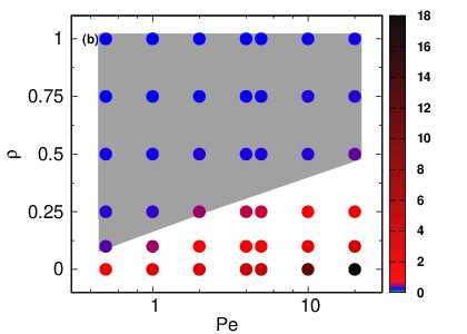
In the previous section, we have identified the nature of the dynamics of the ribbon through its terminus as a function and . Here, we summarize dynamics of the clamped active ribbon in the parameter space of and . The in-plane-motion is accompanied by a significant planar bending of the ribbon, whereas the out-of-plane dynamics causes twisting of the ribbon. We quantify these states by calculating two local geometric quantities, the bending parameter () and the twisting parameter (). The local bending parameter is given as , where is the tangent vector of the protofilament. The local torsional parameter , where is the local binormal vector as shown in the Fig.1-a. We plot the and in the form of a kymograph, which provides the spatio-temporal variation of the respective quantities in Fig.6. For , the bending kymograph indicates propagation of the bending waves from the basal end to the free end of the filament for both and , indicating that the local bending energy of the ribbon oscillates periodically for both in-plane and out-of-plane oscillations. However, the torsional kymograph shows no pattern in the case of planar oscillations when , whereas it indicates propagation of periodic ‘twisting waves’ in the case of out-of-plane oscillations when .
The spatio-temporal pattern formed by both torsional and bending parameters confirms the presence of out-of-plane motion for and beating motion for large values of . In order to quantitatively distinguish between in-plane and out-of-plane dynamics of the ribbon, we define a global torsional parameter . It is evident from Fig. 7-a that remains close to zero in a planar motion, but becomes a large number for out-of-plane movements. We find that increases linearly for small , and (see Fig. 7-a). In the limit of , is almost constant with and exhibits negligible change. Thus, serves as a good indicator for the out of plane motion of the ribbon.
We use the magnitude of geometric parameter as a parameter to quantify the out-of-plane movement in the parameter space of and . Figure 7-b displays a phase diagram for dynamical phases with help of color map, which shows variation in in different phases. In the diagram, we only indicate those points which provide oscillatory dynamics, i.e., only the values of larger than the critical value. The grey shaded area corresponds to in-plane beating motion, whereas the unshaded region corresponds to the rotational phase. From the phase curve, it shows the large global torsional parameter in the rotational phase (red) and small in the beating phase (blue).
III.5 Role of anisotropic friction
Hydrodynamic interactions are ignored in our simulation, however it plays an important role for the active matter and self-propelled systems Pooley et al. 2007; Yang et al. 2008; Brumley et al. 2014. In case of the rod-like filament, friction is anisotropic in the presence of hydrodynamic interactions. Our approach assumes friction to be isotropic thus diffusion too. To verify the universality of our results, we incorporate anisotropic friction to be in the same framework of our simulations, in the absence of hydrodynamic interactions. Thus, the friction parallel and perpendicular to the bond-vectors are taken to be , similar to a filament in solvent Tirado et al. 1984; Doi and Edwards 1988. This effectively modifies diffusivity of the filament in both directions, and mimics the role of hydrodynamics in a very averaged manner. We present here results for at , and , and vary Péclet number to study the behavior of the filament with new protocol.

We present the oscillation frequency of the filament in Fig. 8 under assumption of anisotropic friction. It displays that oscillation frequency varies with power law as with exponent similar to the isotropic friction case, for and . Although values of the oscillation frequencies are different than the isotropic case, however the characteristic features of the results are same. The beating phase and rotational motion is also observed here, thus the results presented in this article are consistent with the anisotropic friction of the filament.
IV Summary and conclusions
In this article, we have presented a systematic study of the dynamics of an active ribbon, clamped at one end which oscillates due to the follower force mechanism. We have identified the mechanical regime in which the modelled ribbon mimics the flagellar motion. We have also analyzed both in-plane and out-of-plane oscillatory motions of the ribbon. The torsion parameter acts as a control parameter in the model, which dictates the transition from in-plane to out-of-plane movement.
We have characterized the periodic oscillations of the ribbon by three different measurements. First, we have calculated the oscillation frequency, which follows the scaling relation for all values of the torsional parameter . We observed only a weak dependence of on . The qualitative difference in the oscillations is manifested in the distributions of angle between clamped-to-free end vector and vertical axis. While the planar beating motion is linked to a broad distribution of angle , the rotational motion leads to a peak about an angle . The width of the distribution increases with . Third, we have visualized the transition from in-plane to out-of-plane motion by analyzing the trajectories of the free-end segment of the ribbon on the PCA transformed planes. By this, we have shown that the trajectory of the free end of the ribbon exhibits intricate dynamical patterns, including butterfly, elliptical, and circular trajectories.
Finally, we have identified the regions in the parameter space defined by and , where different types of oscillations take place. For this purpose, we have estimated the binormal correlation and a geometric torsional parameter . Oscillations in identifies the rotation of the filament. Our analysis reveals that the planar beating and the rotational motion depend on torsional rigidity of the ribbon (via ) as well as the compressive force (via ). For small values of , filament shows rotational motion for all values of , whereas at large the ribbon exhibits beating motion. At the intermediate values of , the oscillatory behavior depends crucially on the magnitude of . We have also shown that torsional energy shows periodic oscillations as a consequence of the rotation of the filament, which disappears in beating phase, whereas planar bending energy always exhibits periodic behavior.
Our study provides an insight into how the oscillatory dynamics of a beating filament changes qualitatively by altering the strength of internal elastic elements. This study helps to design the synthesis of artificial flagella/cilia to be used in micro-scale structures. Although the internal driving mechanism of natural flagella/cilia are fundamentally different, our study hints at the importance of the arrangement of the structural elements in determining their planar beating dynamics. We also show that by tuning the torsional rigidity of a beating filament, one can qualitatively alter the oscillatory pattern of a filament. An eukaryotic flagellum beats due to the active stress generated on the axoneme by molecular motors Lindemann and Lesich 2010; Lindemann 2004; Brokaw 1971; Cibert and Heck 2004. Simulation models including explicit coarse-grained motors acting on the assembly of filaments may provide more insights into dynamical states of the axoneme. It’s worth to consider such systems in the future studies in a more intricate manner.
V Acknowledgements
The computation work is carried out at HPC facility in IISER Bhopal. SPS acknowledges DST SERB Grant No. YSS/2015/000230 for financial support. RC acknowledges DST SERB for financial support via Ramanujan fellowship No. SB/S2/RJN-051/2015.
References
- Marchetti et al. (2013) M. C. Marchetti, J. F. Joanny, S. Ramaswamy, T. B. Liverpool, J. Prost, M. Rao, and R. A. Simha, Rev. Mod. Phys. 85, 1143 (2013).
- Elgeti et al. (2015) J. Elgeti, R. G. Winkler, and G. Gompper, Reports on progress in physics 78, 056601 (2015).
- Bechinger et al. (2016) C. Bechinger, R. Di Leonardo, H. Löwen, C. Reichhardt, G. Volpe, and G. Volpe, Reviews of Modern Physics 88, 045006 (2016).
- Lauga and Powers (2009) E. Lauga and T. R. Powers, Reports on Progress in Physics 72, 096601 (2009).
- Cates (2012) M. E. Cates, Reports on Progress in Physics 75, 042601 (2012).
- Ramaswamy (2010) S. Ramaswamy, Annual Review of Condensed Matter Physics 1, 323 (2010).
- Brennen and Winet (1977) C. Brennen and H. Winet, Annual Review of Fluid Mechanics 9, 339 (1977).
- Palacci et al. (2010) J. Palacci, C. Cottin-Bizonne, C. Ybert, and L. Bocquet, Physical Review Letters 105, 088304 (2010).
- Jiang et al. (2010) H.-R. Jiang, N. Yoshinaga, and M. Sano, Physical review letters 105, 268302 (2010).
- Bricard et al. (2013) A. Bricard, J.-B. Caussin, N. Desreumaux, O. Dauchot, and D. Bartolo, Nature 503, 95 (2013).
- Geyer et al. (2018) D. Geyer, A. Morin, and D. Bartolo, Nature materials 17, 789 (2018).
- Romanczuk et al. (2012) P. Romanczuk, M. Bär, W. Ebeling, B. Lindner, and L. Schimansky-Geier, The European Physical Journal Special Topics 202, 1 (2012).
- Lauga (2007) E. Lauga, Physical Review E 75, 041916 (2007).
- Cates and Tailleur (2013) M. Cates and J. Tailleur, EPL (Europhysics Letters) 101, 20010 (2013).
- Vicsek et al. (1995) T. Vicsek, A. Czirók, E. Ben-Jacob, I. Cohen, and O. Shochet, Phys. Rev. Lett. 75, 1226 (1995).
- Toner and Tu (1995) J. Toner and Y. Tu, Phys. Rev. Lett. 75, 4326 (1995).
- Ghosh and Gov (2014) A. Ghosh and N. Gov, Biophysical journal 107, 1065 (2014).
- Eisenstecken et al. (2016) T. Eisenstecken, G. Gompper, and R. Winkler, Polymers 8, 304 (2016).
- Jiang and Hou (2014) H. Jiang and Z. Hou, Soft Matter 10, 1012 (2014).
- Isele-Holder et al. (2015) R. E. Isele-Holder, J. Elgeti, and G. Gompper, Soft matter 11, 7181 (2015).
- Laskar and Adhikari (2017) A. Laskar and R. Adhikari, New Journal of Physics 19, 033021 (2017).
- Anand and Singh (2018) S. K. Anand and S. P. Singh, Physical Review E 98, 042501 (2018).
- Isele-Holder et al. (2016) R. E. Isele-Holder, J. Jäger, G. Saggiorato, J. Elgeti, and G. Gompper, Soft Matter 12, 8495 (2016).
- Anand and Singh (2019) S. K. Anand and S. P. Singh, Soft Matter 15, 4008 (2019).
- Chelakkot et al. (2014) R. Chelakkot, A. Gopinath, L. Mahadevan, and M. F. Hagan, Journal of The Royal Society Interface 11, 20130884 (2014).
- Jayaraman et al. (2012) G. Jayaraman, S. Ramachandran, S. Ghose, A. Laskar, M. S. Bhamla, P. B. S. Kumar, and R. Adhikari, Phys. Rev. Lett. 109, 158302 (2012).
- Laskar et al. (2013) A. Laskar, R. Singh, S. Ghose, G. Jayaraman, P. B. S. Kumar, and R. Adhikari, Scientific Reports 3, 1964 (2013).
- De Canio et al. (2017) G. De Canio, E. Lauga, and R. E. Goldstein, Journal of The Royal Society Interface 14, 20170491 (2017).
- Elgeti and Gompper (2013) J. Elgeti and G. Gompper, Proceedings of the National Academy of Sciences 110, 4470 (2013).
- Chakrabarti and Saintillan (2019) B. Chakrabarti and D. Saintillan, Physical Review Fluids 4, 043102 (2019).
- Ling et al. (2018) F. Ling, H. Guo, and E. Kanso, Journal of the Royal Society Interface 15, 20180594 (2018).
- Fatehiboroujeni et al. (2018) S. Fatehiboroujeni, A. Gopinath, and S. Goyal, Journal of Computational and Nonlinear Dynamics 13, 121005 (2018), ISSN 1555-1415.
- Doostmohammadi et al. (2018) A. Doostmohammadi, J. Ignés-Mullol, J. M. Yeomans, and F. Sagués, Nature communications 9, 3246 (2018).
- Ndlec et al. (1997) F. Ndlec, T. Surrey, A. C. Maggs, and S. Leibler, Nature 389, 305 (1997).
- Schaller et al. (2010) V. Schaller, C. Weber, C. Semmrich, E. Frey, and A. R. Bausch, Nature 467, 73 (2010).
- Sanchez et al. (2012) T. Sanchez, D. T. Chen, S. J. DeCamp, M. Heymann, and Z. Dogic, Nature 491, 431 (2012).
- Lindemann and Lesich (2010) C. B. Lindemann and K. A. Lesich, J Cell Sci 123, 519 (2010).
- Lindemann (2004) C. B. Lindemann, Biology of the Cell 96, 681 (2004).
- Sleigh (1968) M. Sleigh, in Symposia of the Society for Experimental Biology (1968), vol. 22, pp. 131–150.
- Vilfan et al. (2019) A. Vilfan, S. Subramani, E. Bodenschatz, R. Golestanian, and I. Guido, Nano Letters 19, 3359 (2019), pMID: 30998020.
- Fulford and Blake (1986) G. R. Fulford and J. R. Blake, Journal of theoretical Biology 121, 381 (1986).
- Nonaka et al. (2002) S. Nonaka, H. Shiratori, Y. Saijoh, and H. Hamada, Nature 418, 96 (2002).
- Sawamoto et al. (2006) K. Sawamoto, H. Wichterle, O. Gonzalez-Perez, J. A. Cholfin, M. Yamada, N. Spassky, N. S. Murcia, J. M. Garcia-Verdugo, O. Marin, J. L. Rubenstein, et al., Science 311, 629 (2006).
- Shields et al. (2010) A. R. Shields, B. L. Fiser, B. A. Evans, M. R. Falvo, S. Washburn, and R. Superfine, Proceedings of the National Academy of Sciences 107, 15670 (2010), ISSN 0027-8424.
- Sanchez et al. (2011) T. Sanchez, D. Welch, D. Nicastro, and Z. Dogic, Science 333, 456 (2011).
- Nishiguchi et al. (2018) D. Nishiguchi, J. Iwasawa, H.-R. Jiang, and M. Sano, New Journal of Physics 20, 015002 (2018).
- Dreyfus et al. (2005) R. Dreyfus, J. Baudry, M. L. Roper, M. Fermigier, H. A. Stone, and J. Bibette, Nature 437, 862 (2005).
- Giomi and Mahadevan (2010) L. Giomi and L. Mahadevan, Physical review letters 104, 238104 (2010).
- Sarkar and Thakur (2017) D. Sarkar and S. Thakur, The Journal of chemical physics 146, 154901 (2017).
- Yang et al. (2018) Q.-s. Yang, Q.-w. Fan, Z.-l. Shen, Y.-q. Xia, W.-d. Tian, and K. Chen, The Journal of chemical physics 148, 214904 (2018).
- Saggiorato et al. (2017) G. Saggiorato, L. Alvarez, J. F. Jikeli, U. B. Kaupp, G. Gompper, and J. Elgeti, Nature Communications 8, 1415 (2017).
- Jolliffe (2005) I. Jolliffe, Principal Component Analysis (American Cancer Society, 2005), ISBN 9780470013199.
- Werner et al. (2014) S. Werner, J. C. Rink, I. H. Riedel-Kruse, and B. M. Friedrich, PloS one 9, e113083 (2014).
- Stephens et al. (2008) G. J. Stephens, B. Johnson-Kerner, W. Bialek, and W. S. Ryu, PLoS computational biology 4, e1000028 (2008).
- Ma et al. (2014) R. Ma, G. S. Klindt, I. H. Riedel-Kruse, F. Jülicher, and B. M. Friedrich, Physical review letters 113, 048101 (2014).
- Golestanian and Liverpool (2000) R. Golestanian and T. B. Liverpool, Physical Review E 62, 5488 (2000).
- Liverpool et al. (1998) T. B. Liverpool, R. Golestanian, and K. Kremer, Physical review letters 80, 405 (1998).
- Pooley et al. (2007) C. Pooley, G. Alexander, and J. Yeomans, Physical review letters 99, 228103 (2007).
- Yang et al. (2008) Y. Yang, J. Elgeti, and G. Gompper, Physical Review E 78, 061903 (2008).
- Brumley et al. (2014) D. R. Brumley, K. Y. Wan, M. Polin, and R. E. Goldstein, Elife 3, e02750 (2014).
- Tirado et al. (1984) M. M. Tirado, C. L. Martínez, and J. G. de la Torre, The Journal of chemical physics 81, 2047 (1984).
- Doi and Edwards (1988) M. Doi and S. F. Edwards, The theory of polymer dynamics, vol. 73 (oxford university press, 1988).
- Brokaw (1971) C. J. Brokaw, Journal of Experimental Biology 55, 289 (1971).
- Cibert and Heck (2004) C. Cibert and J.-V. Heck, Cell motility and the cytoskeleton 59, 153 (2004).
Supplementary Text
The binormal persistence length () of the ribbon for various torsional strength is displayed in the Fig. SI-1. It is estimated from the binormal-binormal correlation given as, . Interestingly, the persistence length varies linearly with . The increase in the persistence length suggests the strengthening of torsional rigidity of the ribbon with .


The ratio of mean of amplitudes of the periodic motion on the x-z plane defined as (the direction along beating plane, and perpendicular to the beating plane) as shown in Fig. SI-1-b. If this ratio is small, it suggests amplitude in x-direction is much more than that in -direction, and the trajectory is linear along -axis. If this ratio is close to one, it suggests that amplitudes in x-direction and in -direction are same, and the trajectory can be circular. For lower values of , i.e. , amplitudes is close to one, therefore shape of trajectory is nearly circular. Further, intermediate value of gives elliptical trajectory. For , grows from a small value to one, and eventually reaches to the transition towards the butterfly to elliptical trajectory. For the higher torsion ratio, i.e., , is very small suggesting motion is on the x-y plane only, this suggests end-monomer moves nearly along the x-axis. With , shifts progressively towards the higher values. The trajectory of the end monomer may become circular again in the large compressive force limit. This also confirms that the transition between beating to rotation is not sudden, it changes continuously with increasing compressive force. As Fig. SI-1-b suggests, transition from beating to rotation follows the path of butterfly to circular via elliptical trajectory.


We present here the discussion and the quantification of oscillation frequency through deflection of the ribbon in x-direction. The deflection is caused by bending of the filament, therefore measured frequency in this way quantifies only bending oscillations. Further, we analyse the oscillation frequency via the azimuthal angle of the ribbon’s terminus end. This quantity can provide out-of plane oscillations at small . In this limit, i.e., at the oscillation of azimuthal angle coincides with the oscillation in x-deflection as illustrated in Fig. SI-2-a. When , we observe local oscillations in the torsional parameter as given in Fig. 6-c of the main text. The frequency of oscillations in bending energy is computed by the Fourier transformation of the time evolution of for different values of . Similarly, we also obtain frequency from oscillation in torsional energy . Frequencies from torsional and azimuthal’s angle coincides with the bending frequency Fig. SI-2-b.