Implicit Progressive-Iterative Approximation for Curve and Surface Reconstruction
Abstract
Implicit curve and surface reconstruction attracts the attention of many researchers and gains a wide range of applications, due to its ability to describe objects with complicated geometry and topology. However, extra zero-level sets or spurious sheets arise in the reconstruction process makes the reconstruction result challenging to be interpreted and damage the final result. In this paper, we proposed an implicit curve and surface reconstruction method based on the progressive-iterative approximation method, named implicit progressive-iterative approximation (I-PIA). The proposed method elegantly eliminates the spurious sheets naturally without requiring any explicit minimization procedure, thus reducing the computational cost greatly and providing high-quality reconstruction results. Numerical examples are provided to demonstrate the efficiency and effectiveness of the proposed method.
Keywords:
Implicit curve and surface, Curve and surface fitting, Progressive-iterative approximation.1 Introduction
Implicit representation and parametric representation are two common representation techniques in geometric design. With parametric representations, it is difficult to fit a data set with complicated geometry, and parametrization is always a challenging problem. Without requiring any parametrization, the implicit function can describe an object with complicated geometry and supply flexible and smooth surface representation. Thus, implicit surface reconstruction receives great attention due to its capability to create an object with complicated topology and geometry.
However, the extra zero-level sets generated in the implicit curve and surface reconstruction procedure make the reconstruction results challenging to be interpreted and damage the resulting curve and surface. To eliminate the extra zero-level sets, regularization terms are usually required to be added in the objective functions of minimization problems for implicit curve and surface reconstruction. For example, Liu [1] incorporated the total variation of implicit representation to reduce the appearance of the extra zero-level sets as minimum as possible. In Refs. [2, 3, 4, 5], tension terms are added in the minimization problem to get rid of extra zero-level sets and avoid a singular system of equations. Because the forms of the regularization terms are usually complicated, their addition to the objective functions seriously affects the efficiency of the implicit curve and surface reconstruction algorithms.
On the other hand, progressive-iterative approximation (PIA) is a series of efficient data fitting methods with intuitive geometric meaning. They have been extensively employed in parametric curve and surface fitting, and subdivision curve and surface fitting [6, 7, 8, 9, 10, 11, 12, 13, 14, 15], but never been used in implicit curve and surface reconstruction. In this paper, we developed a progressive-iterative approximation method for implicit curve and surface reconstruction, named implicit progressive-iterative approximation (I-PIA). We proved the convergence of I-PIA, and showed that the I-PIA method itself naturally solves a minimization problem with a regularization term, without any extra computation effort. Therefore, not only the I-PIA method can eliminate the extra level sets, but, more importantly, it can improve the reconstruction efficiency of the implicit curves and surfaces. Lots of numerical examples illustrated in this paper show that, by I-PIA, the implicit curve and surface reconstruction time is improved one to three orders of magnitude, compared with the state-of-the-art implicit curve and surface reconstruction methods. In conclusion, the main contributions of this paper include:
- 1.
I-PIA naturally solves a minimization problem with a regularization term in its iteration procedure, without any extra computation effort.
- 2.
No extra zero-level sets exist in the iteration of I-PIA, so the reconstruction result by I-PIA is very clear.
- 3.
The implicit curve and surface reconstruction time by I-PIA is improved at least one to three orders of magnitude, compared with the state-of-the-art methods.
The structure of this paper is as follows. In Section 1.1, we reviewed some related work. Preliminary definitions and statements of the problems are given in Section 2. In Section 3, we presented the I-PIA method for implicit curve and surface reconstruction. Experimental results and discussions are given in Section 4. Finally, we conclude the paper in Section 5.
1.1 Related work
In this section, some work related to implicit curve and surface reconstruction and progressive iterative approximation (PIA) will be briefly reviewed.
Implicit curve and surface reconstruction: Most implicit surface reconstruction algorithms blend local implicit primitives to represent surfaces based on the idea developed by Blinn [16]. Muraki [17] developed the Blobby model to fit a very complicated data set by blending implicit primitives. Hoppe et al. [18] proposed a surface reconstruction algorithm based on the locally defined signed distance function. Curless and Levoy [19] used the volumetric representation consisting of a cumulative weighted signed distance function. Carr et al. [20] proposed a fast method for fitting and evaluating Radial basis functions (RBFs) to model a large data set.
So far, many schemata had been considered to reduce the amount of storage cost in implicit reconstruction. Morse [21] proposed using compactly supported radial basis functions to reduce the computational cost and memory requirement, which allows reconstructing surface from large data-sets that are impractical from the previous method like [22]. Furthermore, Refs. [23, 24] consider compactly supported RBF to reduce the computational cost and improve the efficiency of the reconstruction process. Pan et al. [25] incorporated a low-rank tensor approximation technique and reduced the storage requirement efficiently.
Ohtake et al. [26] proposed a multi-level partition of unity (MPU) representation to reconstruct surface models from a huge set of points. Wang et al. [27] presented a surface reconstruction algorithm based on the implicit PHT-spline, which reconstructs a surface from a large point cloud efficiently. The Poisson surface reconstruction proposed by Kazhdan et al. [28] expresses the surface reconstruction as a Poisson problem and approximates the indicator function of the surface. Moreover, screened Poisson surface reconstruction was presented to avoid the over-smoothing by incorporating the positional constraints in the optimization problem [29].
Progressive iterative approximation (PIA): PIA is widely used for its ability to fit data efficiently. PIA method elegantly generates a sequence of curves/surfaces by refining the control points of blending curves/surfaces, and the data points are interpolated by the limit of the sequence. Both the numbers of control points and data points are required to be equal in the classical PIA. With the recent advancement of the big data era, it is infeasible to fit large-scale data points by PIA. To overcome this drawback, Lin and Zhang [13] developed an extended PIA (EPIA) method, which allows the number of data points to be higher than the number of control points. Progressive and iterative approximation for least square fitting (LSPIA) [8] is another elegant PIA method, which allows the number of data points to be higher than the number of control points, and its limit is the least square fitting result to a given data set.
Initially, Qi et al. [30] and de Boor [31] discovered the property of PIA for uniform cubic B-spline curve. Later, Lin et al. [12] showed that non-uniform B-spline curve and surface have PIA property. Moreover, PIA property holds for curves and surfaces with normalized totally positive (NTP) basis [14]. Also Rational B-spline curve and surface posses this property [32]. Lu [15] proposed a weighted PIA technique to increase the convergence rate of the PIA method. For more details, a comprehensive overview of PIA is provided in [33].
As stated above, some PIA methods have been developed for both parametric curve and surface fitting, and subdivision curve and surface fitting, but never been used in implicit curve and surface reconstruction.
2 Definitions and preliminaries
In this section, statement of the problems, definition of implicit B-spline curve and surface are given. Specifically, the following problems will be handled in this paper.
Implicit curve reconstruction problem: Given a collection of unorganized data points in the two-dimensional space,
| (1) |
with a set of associated oriented unit normals , find a function so that the zero level sets of , i.e., , fit the unorganized point set (1).
Implicit surface reconstruction problem: Given a collection of unorganized data points in the three-dimensional space,
| (2) |
with a set of associated oriented unit normals , find a function so that the zero level sets of , i.e., , fit the unorganized point set (2).
Let be a bivariate tensor-product B-spline function of bi-degree defined over some domain [1, 5]:
| (3) |
where are the control coefficients and are the B-spline basis functions with some given knot sequences. We consider the bi-cubic B-spline functions, i.e. with uniform knot sequences. The implicit B-spline curve reconstructed by fitting the data point set (1) is given by
| (4) |
Similarly define the trivariate tensor product B-spline function on some domain as [1, 5]:
| (5) |
where are the control coefficients, and are the B-spline basis functions. In our implementation, the tri-cubic B-spline function is employed. Analogously, the implicit B-spline surface reconstructed by fitting the data point set (2) is,
| (6) |
For simplicity, we only present the method for implicit curve reconstruction in the following, and that for the implicit surface reconstruction is similar. Actually, the implicit curve is reconstructed by minimizing the sum of the squared algebraic distances [2], i.e.,
| (7) |
where are the coefficients of the tensor product B-spline function. However, in the implicit curve and surface reconstruction problem, the minimization problem (7) is usually underdetermined, i.e., the number of unknowns is larger than that of the data points, thus leading to extra zero level sets in the reconstruction results.
To make the undetermined problem (7) determined, and eliminate the extra zero level sets, global regularization terms are added in the minimization problem (7) [2, 3, 4, 5]. However, the addition of the regularization terms seriously affects the efficiency of implicit curve and surface reconstruction. In this paper, we developed the I-PIA method for implicit curve and surface reconstruction, which solves the minimization problem with regularization terms naturally, and improves the efficiency of implicit curve and surface reconstruction significantly, while eliminating the extra zero level sets.
3 Implicit progressive iterative approximation
In this section, we will develop the I-PIA iteration method for the implicit curve and surface reconstruction, and prove its convergence.
3.1 I-PIA for implicit curve reconstruction
Given the unorganized data point set (1), with a set of associated oriented unit normals , we want to reconstruct an implicit curve from the data point set. To avoid the trivial solution, we need to add extra offset points to the data point set (1). The offset points are generated along the normal vector at small distance [20, 34, 4], i.e.,
Let be the value of the implicit function at the offset points, i.e.,
Define the initial implicit B-spline function as follows:
| (8) |
where the initial control coefficients are taken as .
Let be the difference vectors for the data points, which can be calculated as,
Moreover, let be the difference vectors for the control coefficients, defined as,
where, is a weight, and its selection method is explained in Remark 3.1. The new coefficients are obtained by:
and the new implicit B-spline curve,
Likewise, suppose we have obtained the -th implicit curves after the -th iteration, and let,
| (9) |
| (10) |
From the above iterative procedure, we generate a series of implicit B-spline functions .
Now, arrange the control coefficients to a vector in the lexicographic order, i.e.,
and let,
According to (9), we have
Then, the I-PIA (9) for implicit curve reconstruction can be represented in the matrix form,
| (11) | |||||
where, is the collocation matrix of the basis functions (arranged in the lexicographical order),
on the point sequence , i.e.,
| (12) |
Remark 3.1
3.2 I-PIA for implicit surfaces reconstruction
The I-PIA iterative method for the implicit curve reconstruction can be easily extended to implicit surface reconstruction. In the following, the details of I-PIA for implicit surface reconstruction will be presented.
Given the unorganized data point set (2), with a set of associated oriented unit normals , we want to reconstruct an implicit surface from the data point set. To avoid the trivial solution, extra offset point should be added to the data point set (2). The offset points are generated along the normal vector at small distance [20, 34, 4], i.e.,
Moreover, let be the value of the implicit function at the offset points, i.e.,
Define the initial B-spline implicit function as follows:
where . Let be the difference vectors for the data points, calculated by,
Then, the difference vectors for the control coefficients can be constructed as,
where, is a weight, and its selection method is explained in Remark 3.2. Similar as the curve case, we can get the new coefficients,
and the new implicit B-spline surface,
| (13) |
Likewise, suppose we have obtained the -th implicit B-spline surface after the -th iteration, and let,
| (14) |
| (15) |
In this way, a series of implicit B-spline surface is generated.
Similar as the curve case in Section 3.1, arranging the control coefficients
to a vector in the lexicographic order, i.e.,
and letting,
The I-PIA (14) for implicit surface reconstruction can be represented in the matrix form,
| (16) | |||||
where, is the collocation matrix of the basis functions (arranged in the lexicographical order),
on the point sequence , i.e.,
| (17) |
Remark 3.2
3.3 Convergence analysis
As shown above, the I-PIA iteration method for implicit curve reconstruction (11) and that for implicit surface reconstruction (16) can be represented in a unified form, i.e.,
| (18) |
The matrices in Eqs. (11) and (16) hold some common properties:
- Property 1:
The matrix is positive semi-definite. So, its eigenvalues are nonnegative real numbers.
- Property 2:
The matrix is singular. In the implicit B-spline curve and surface reconstruction, the number of data points (suppose it is ) is less than that of the control coefficients of implicit curve and surface (suppose ), i.e, . Because the order of the matrix is , its rank is at most . So the rank of the matrix is at most (). It means that the matrix is singular.
- Property 3:
The eigenvalues of satisfy . This is because the choice of the weight , as well as Properties 1 and 2.
Remark 3.3
According to Property 2, the matrix is singular. Suppose the dimension of its zero eigenspace is . Then, the rank of the matrices and is,
On the other hand, the implicit curve and surface reconstruction problem can be formulated as solving the following least-squares fitting problem,
| (19) |
where is an unknown vector, and are the same as in Eq. (18). As pointed out by Property 2, the coefficient matrix is singular. So, if the solution of the least-square fitting system (19) exists, it has infinite solutions, which usually leads to extra zero-level sets. Therefore, to eliminate the extra zero-level sets and get desirable results, it is required to solve the constrained minimization problem,
| (20) |
where, is the Euclidean norm, or its variants. In the following, we will show that, the I-PIA iterative method (18) converges to the solution of the constrained minimization problem (20).
Theorem 3.4
Proof: By Remark 3.3, . Because the matrix is both a normal matrix and a positive semi-definite matrix, its eigen decomposition and singular value decomposition are the same,
| (21) |
where is an orthogonal matrix, and are both the eigen values and singular values of the matrix . Then, the M-P inverse of is,
Therefore, we have,
Due to Eq. (21), it holds,
where are the eigen values of the matrix . Based on Property 3, they satisfy . Therefore,
| (22) |
Note that the linear system has solutions, if and only if [35],
| (23) |
Then, subtracting from both sides of Eq. (18), leads to,
So, together with Eqs. (22) and (23), we have,
Therefore,
which are the solutions of the singular linear system (note that can take an arbitrary value). Among them, is the one with minimum Euclidean norm. So, when the initial value , the I-PIA iterative format converges to , the solution of the singular linear system with the minimum Euclidean norm. It is the solution of the constrained minimization problem (20).


4 Experiments and discussion
Several experiments have been carried out to evaluate the performance of I-PIA. All the experiments are performed in MATLAB on a PC with an Intel-core i7 @ 3.6 GHz processor and 16 GB of RAM. The results and discussions specifically focus on the following areas: effectiveness, robustness to inaccurate distance field, hole filling, non-uniform sampling and noisy data, porous surface (open surface), and fine details. The statistical of I-PIA, as well as the comparison with the state-of-the-art method [1], is listed in Tables 1 and 2.
4.1 Effectiveness
As stated above, the extra zero-level sets generated in the implicit curve and surface reconstruction procedure make the reconstruction results challenging to be interpreted, and the elimination of extra zero-level sets is the main problem in designing implicit curve and surface reconstruction method. With the I-PIA developed in this paper, no extra zero-level set appears in the reconstruction procedure. To show the effectiveness of I-PIA in the reconstruction of implicit curves and surfaces without the appearance of extra level sets, we test our algorithm on planar curves and 3D surfaces. The initial control coefficients are taken as zero. After every iteration, the control coefficients are updated and refined by the difference vectors for the control coefficient, and the resulting implicit curve/surface will approach the given data sets closer than the previous implicit curve/surface.
Fig. 1 shows the reconstruction process of two data sets. Similarly, Fig. 2 illustrates the reconstruction process of two data sets. From the results presented in Fig. 1 and Fig. 2, we can see that no extra zero-level sets exist in the reconstruction process of the and data sets.


4.2 Robustness to inaccurate distance field
The auxiliary offset points appended to the data points helps to orient the surface and avoid the appearance of artifacts in curve and surface reconstruction [20, 1]. The I-PIA algorithm is insensitive to the distance values assigned at the offset points, thus robust to the inaccurate distance field. The first row of Fig. 3 illustrates the reconstruction of a data sets with synthesis offset points. The function values on the offset points are assigned in a random strategy. That is, the preassigned values are selected as uniformly distributed random numbers in for the outside offsets and for the inside offset, respectively, where , as demonstrated in Figs. 3(b)- 3(e). The results show that I-PIA can still reconstruct the given data sets in a corrupted distance field.
Moreover, given a data points set, we generate two sets of offset points inside and outside the data points set respectively. However, the distance values are assigned in reverse order, i.e., larger distance values are given to nearer offset points, and smaller distance values are given to far offset points. As illustrated in Figs. 3(f) and 3(h), from inside to outside, the distance values of the four sets of offset points are . The curves is robustly reconstructed using I-PIA, and demonstrated in Figs. 3(g) and 3(i).
4.3 Holes filling
Holes and missing data often arise in the point cloud generated by scanning devices. Fig. 4 (a)–(c) depicts the reconstructed surfaces of elephant, fertility, and bunny respectively, in which some portions of the data points are removed to creates holes and gaps. The reconstructed surfaces are illustrated in the first row, and the second row shows the reconstructed surfaces with the data points superimposed. As can be seen, I-PIA successfully filled the holes and gaps. Thus, I-PIA performs well in filling holes and missing data.


4.4 Non-uniform sampling and noisy data
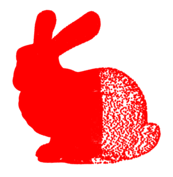
In this section, we demonstrates the capability of I-PIA in handling non-uniform sampling and noisy data. In Fig. 5, the original point cloud of the bunny model is illustrated. In Fig. 5, the right part of the bunny model is down-sampled, and of the original data points are removed. Moreover, in Fig. 5, the data points are disturbed by noise. However, by I-PIA, the input point clouds in Fig. 5 and Fig. 5 do not cause artifacts in the reconstructed surfaces in Fig. 5 and Fig. 5, respectively.
The features and details of the reconstructed surface by I-PIA depends on the mesh grid used. If the density of the input point cloud is reduced, I-PIA can still reconstruct the surface with fine details and features if the mesh grid is refined. Fig. 6 shows the reconstructed surfaces from the point clouds of the model armadillo with different density, where Fig. 6 is the original point cloud, and Fig. 6 is the law density point cloud with points of the original point cloud. While the reconstructed surface from the original point cloud, which is based on a coarse grid , is illustrated in Fig. 6, the reconstructed surface from the low density point cloud, based on a fine grid , is demonstrated in Fig. 6. It can be seen that, though the density of the point cloud is lower than that of the original one, the reconstructed surface with finer grid captures more details and features.



4.5 Open surface (Porous surface)
I-PIA can perform well for the reconstruction of the open surfaces. Fig. 7 depict the reconstructed surface of gyroid, a kind of porous surface. From left to right of Fig. 7, there are the given point cloud, reconstructed surface, and reconstructed surface with the given data superimposed, respectively. It can be seen that the implicit B-spline surface reconstructed by I-PIA conforms to the given point cloud well.


4.6 Fine details
To show the level of quality of the surfaces reconstructed by our algorithm, we enlarged some parts of Buddha and BU in Fig. 8. The features of the models are correctly recovered using I-PIA.
| Model | Number of data point | Grid size | Maximum Error | Time | |
|---|---|---|---|---|---|
| Flower | 509 | 2.924–3 | 1.88 | ||
| Coons curve | 780 | 1.2524–3 | 2.05 | ||
| Dolphin | 371 | 3.2457–3 | 1.67 | ||
| Butterfly | 508 | 2.8881–3 | 1.79 |
| Model | Data point | Grid size | Maximum Error | Method in [1] | I-PIA | ||
|---|---|---|---|---|---|---|---|
| Time | Time | ||||||
| Double-torus | 766 | 1.0574–3 | 90.07 | 3.61 | |||
| Torus | 10100 | 3.0412–6 | 189.13 | 8.22 | |||
| Gyroid | 36627 | 4.8708–6 | 11149.28 | 34.26 | |||
| Elephant | 52100 | 9.6839–4 | 2773.65 | 44.55 | |||
| Bunny | 35947 | 9.5983–2 | 26428.69 | 88.24 | |||
| Fertility | 241607 | 9.5989–5 | 25298.49 | 902.35 | |||
| Armadillo | 51892 | 1.9831–2 | 24hr | 2732.32 | |||
| Buddha | 80000 | 7.4594–2 | 24hr | 1835.73 | |||
| Bu | 70000 | 1.1899–3 | 24hr | 2028.01 |
4.7 Performance
Table 1 summarizes the running time performance of I-PIA on different planner curves. Table 2 shows the comparison of running time performance of I-PIA and the state-of-the-art method in [1]. The computational cost of [1] is higher than that of I-PIA, because in each iteration of the method in [1], a linear system needs to be solved, while I-PIA avoids solving the linear system. The surface reconstructions of Armadillo, Buddha, and BU are not completed in 24 hours using the method in [1]. In summary, the implicit curve and surface reconstruction time by I-PIA is improved at least one to three orders of magnitude, compared with the state-of-the-art method in [1].
5 Conclusions
In this paper, we proposed a novel approach for implicit curve and surface reconstruction based on the progressive-iterative approximation method, named I-PIA. I-PIA solves the minimization problem with regularization terms naturally without any extra computation effort. Thus, it not only avoids the spurious sheets and artifacts but also reduces the computational cost effectively. Several kinds of experiments presented demonstrate that I-PIA is robust to inaccurate distance field, data holes, non-uniform sampling and point noise, and thus produces high-quality reconstruction results.
Acknowledgments
This work is supported by the National Natural Science Foundation of China under Grant No.61872316, and the National Key R&D Plan of China under Grant No.2016YFB1001501.
References
- [1] Y. Liu, Y. Song, Z. Yang, J. Deng, Implicit surface reconstruction with total variation regularization, Computer Aided Geometric Design 52 (2017) 135–153.
- [2] B. Jüttler, A. Felis, Least-squares fitting of algebraic spline surfaces, Advances in Computational Mathematics 17 (1-2) (2002) 135–152.
- [3] M. Rouhani, A. D. Sappa, Implicit B-spline fitting using the 3L algorithm, in: 2011 18th IEEE International Conference on Image Processing, IEEE, 2011, pp. 893–896.
- [4] M. Rouhani, A. D. Sappa, E. Boyer, Implicit B-spline surface reconstruction, IEEE Transactions on Image Processing 24 (1) (2014) 22–32.
- [5] Z. Yang, J. Deng, F. Chen, Fitting unorganized point clouds with active implicit B-spline curves, The Visual Computer 21 (8-10) (2005) 831–839.
- [6] Z. Chen, X. Luo, L. Tan, B. Ye, J. Chen, Progressive interpolation based on Catmull-Clark subdivision surfaces, Computer Graphics Forum 27 (7) (2008) 1823–1827.
- [7] F.-H. F. Cheng, F.-T. Fan, S.-H. Lai, C.-L. Huang, J.-X. Wang, J.-H. Yong, Loop subdivision surface based progressive interpolation, Journal of Computer Science and Technology 24 (1) (2009) 39–46.
- [8] C. Deng, H. Lin, Progressive and iterative approximation for least squares B-spline curve and surface fitting, Computer-Aided Design 47 (2014) 32–44.
- [9] C. Deng, W. Ma, Weighted progressive interpolation of Loop subdivision surfaces, Computer-Aided Design 44 (5) (2012) 424–431.
- [10] H. Lin, Local progressive-iterative approximation format for blending curves and patches, Computer Aided Geometric Design 27 (4) (2010) 322–339.
- [11] H. Lin, Q. Cao, X. Zhang, The convergence of least-squares progressive iterative approximation with singular iterative matrix, arXiv preprint arXiv:1707.09109.
- [12] H. Lin, G. Wang, C. Dong, Constructing iterative non-uniform B-spline curve and surface to fit data points, Science in China Series: Information Sciences 47 (3) (2004) 315–331.
- [13] H. Lin, Z. Zhang, An extended iterative format for the progressive-iteration approximation, Computers & Graphics 35 (5) (2011) 967–975.
- [14] H.-W. Lin, H.-J. Bao, G.-J. Wang, Totally positive bases and progressive iteration approximation, Computers & Mathematics with Applications 50 (3-4) (2005) 575–586.
- [15] L. Lu, Weighted progressive iteration approximation and convergence analysis, Computer Aided Geometric Design 27 (2) (2010) 129–137.
- [16] J. F. Blinn, A generalization of algebraic surface drawing, ACM Transactions on Graphics (TOG) 1 (3) (1982) 235–256.
- [17] S. Muraki, Volumetric shape description of range data using “blobby model”, ACM SIGGRAPH Computer Graphics 25 (4) (1991) 227–235.
- [18] H. Hoppe, T. DeRose, T. Duchamp, J. McDonald, W. Stuetzle, Surface reconstruction from unorganized points, ACM SIGGRAPH Computer Graphics 26 (2) (1992) 71–78.
- [19] B. Curless, M. Levoy, A volumetric method for building complex models from range images, in: Proceedings of the 23rd Annual Conference on Computer Graphics and Interactive Techniques, ACM, 1996, pp. 303–312.
- [20] J. C. Carr, R. K. Beatson, J. B. Cherrie, T. J. Mitchell, W. R. Fright, B. C. McCallum, T. R. Evans, Reconstruction and representation of 3D objects with radial basis functions, in: Proceedings of the 28th Annual Conference on Computer Graphics and Interactive Techniques, SIGGRAPH ’01, ACM, 2001, pp. 67–76.
- [21] B. S. Morse, T. S. Yoo, P. Rheingans, D. T. Chen, K. R. Subramanian, Interpolating implicit surfaces from scattered surface data using compactly supported radial basis functions, in: ACM SIGGRAPH 2005 Courses, ACM, 2005, p. 78.
- [22] G. Turk, J. F. O’brien, Variational implicit surfaces, Technical Report GIT-GUV-99-15, Georgia Institute of Technology.
- [23] N. Kojekine, I. Hagiwara, V. Savchenko, Software tools using CSRBFs for processing scattered data, Computers & Graphics 27 (2) (2003) 311–319.
- [24] Y. Ohtake, A. Belyaev, H.-P. Seidel, Multi-scale and adaptive CS-RBFS for shape reconstruction from clouds of points, in: Advances in Multiresolution for Geometric Modelling, Springer, 2005, pp. 143–154.
- [25] M. Pan, W. Tong, F. Chen, Compact implicit surface reconstruction via low-rank tensor approximation, Computer-Aided Design 78 (2016) 158–167.
- [26]
Y. Ohtake, A. Belyaev, M. Alexa, M. Alexa, G. Turk, H.-P. Seidel, Multi-level
partition of unity implicits, ACM Trans. Graph. 22 (3) (2003) 463–470.
URL http://doi.acm.org/10.1145/882262.882293 - [27] J. Wang, Z. Yang, L. Jin, J. Deng, F. Chen, Parallel and adaptive surface reconstruction based on implicit PHT-splines, Computer Aided Geometric Design 28 (8) (2011) 463–474.
- [28] M. Kazhdan, M. Bolitho, H. Hoppe, Poisson surface reconstruction, in: Proceedings of the Fourth Eurographics Symposium on Geometry Processing, Vol. 7, 2006, pp. 61–70.
- [29] M. Kazhdan, H. Hoppe, Screened poisson surface reconstruction, ACM Transactions on Graphics (ToG) 32 (3) (2013) 29.
- [30] D. Qi, Z. Tian, Y. Zhang, J. Feng, The method of numeric polish in curve fitting, Acta Mathematica Sinica 18 (3) (1975) 173–184.
- [31] C. de Boor, How does Agee’s smoothing method work, in: Proceedings of the 1979 army numerical analysis and computers conference, ARO Report, 1979, pp. 79–3.
- [32] S. Limin, W. Renhong, An iterative algorithm of NURBS interpolation and approximation, Journal of Mathematical Research and Exposition 26 (4) (2006) 735–743.
- [33] H. Lin, T. Maekawa, C. Deng, Survey on geometric iterative methods and their applications, Computer-Aided Design 95 (2018) 40–51.
- [34] G. E. Fasshauer, Meshfree approximation methods with MATLAB, Vol. 6, World Scientific, 2007.
- [35] M. James, The generalised inverse, The Mathematical Gazette 62 (420) (1978) 109–114.