On a relation between harmonic measure and hyperbolic distance on planar domainsThanks: I thank Professor D. Betsakos, my thesis advisor, for his help and advice during the preparation of this work, and the Onassis Foundation for the scholarship I receive during my Ph.D. studies.

Christina Karafyllia Address: Department of Mathematics, Aristotle University of Thessaloniki, 54124, Thessaloniki, Greece Email address: karafyllc@math.auth.gr

Abstract.

Let $\psi$ be a conformal map of $\mathbb{D}$ onto an unbounded domain and, for $\alpha>0$ , let ${F_{\alpha}}=\left\{{z\in\mathbb{D}:\left|{\psi\left(z\right)}\right|=\alpha}\right\}$ . If $\omega_{\mathbb{D}}\left({0,{F_{\alpha}}}\right)$ denotes the harmonic measure at $0$ of $F_{\alpha}$ and $d_{\mathbb{D}}{\left({0,{F_{\alpha}}}\right)}$ denotes the hyperbolic distance between $0$ and $F_{\alpha}$ in $\mathbb{D}$ , then an application of the Beurling-Nevanlinna projection theorem implies that ${\omega_{\mathbb{D}}}\left({0,{F_{\alpha}}}\right)\geq\frac{2}{\pi}{e^{-{d_{\mathbb{D}}}\left({0,{F_{\alpha}}}\right)}}$ . Thus a natural question, first stated by P. Poggi-Corradini, is the following: Does there exist a positive constant $K$ such that for every $\alpha>0$ , ${\omega_{\mathbb{D}}}\left({0,{F_{\alpha}}}\right)\leq K{e^{-{d_{\mathbb{D}}}\left({0,{F_{\alpha}}}\right)}}$ ? In general, we prove that the answer is negative by means of two different examples. However, under additional assumptions involving the number of components of $F_{\alpha}$ and the hyperbolic geometry of the domain $\psi\left(\mathbb{D}\right)$ , we prove that the answer is positive.

Key words and phrases:

Harmonic measure, Extremal length, Conformal mapping, Hyperbolic distance, Domain decomposition method, Hardy space

2010 Mathematics Subject Classification

Primary 30C85, 30F45, 31A15

1 Introduction

We will give an answer to a question of P. Poggi-Corradini ([17, p. 36]) about an inequality relating harmonic measure and hyperbolic distance. For a domain $D$ , a point $z\in D$ and a Borel subset $E$ of $\overline{D}$ , let ${\omega_{D}}\left({z,E}\right)$ denote the harmonic measure at $z$ of $\overline{E}$ with respect to the component of $D\backslash{\overline{E}}$ containing $z$ . The function ${\omega_{D}}\left({\cdot,E}\right)$ is exactly the solution of the generalized Dirichlet problem with boundary data $\varphi={1_{E}}$ (see [1, ch. 3], [8, ch. 1] and [19, ch. 4]). The hyperbolic distance between two points $z,w$ in the unit disk $\mathbb{D}$ (see [1, ch. 1], [2, p. 11-28]) is defined by

{d_{\mathbb{D}}}\left({z,w}\right)=\log\frac{{1+\left|{\frac{{z-w}}{{1-z\bar{w}}}}\right|}}{{1-\left|{\frac{{z-w}}{{1-z\bar{w}}}}\right|}}.

It is conformally invariant and thus it can be defined on any simply connected domain $D\neq\mathbb{C}$ as follows: If $f$ is a Riemann map of $\mathbb{D}$ onto $D$ and $z,w\in D$ , then ${d_{D}}\left({z,w}\right)={d_{\mathbb{D}}}\left({{f^{-1}}\left(z\right),{f^{-1}}\left(w\right)}\right)$ . Also, for a set $E\subset D$ , we define ${d_{D}}\left({z,E}\right):=\inf\left\{{{d_{D}}\left({z,w}\right):w\in E}\right\}$ .

The Hardy space with exponent $p$ , $p>0$ , and norm ${\left\|\cdot\right\|_{p}}$ (see [5, p. 1-2], [8, p. 435-441]) is defined to be

{H^{p}}\left(\mathbb{D}\right)=\left\{{f\in H\left(\mathbb{D}\right):\left\|f\right\|_{p}^{p}=\mathop{\sup}\limits_{0<r<1}\int_{0}^{2\pi}{{{\left|{f\left({r{e^{i\theta}}}\right)}\right|}^{p}}d\theta<+\infty}}\right\},

where $H\left(\mathbb{D}\right)$ denotes the family of all holomorphic functions on $\mathbb{D}$ . The fact that a function $f$ belongs to ${H^{p}}\left(\mathbb{D}\right)$ imposes a restriction on the growth of $f$ and this restriction is stronger as $p$ increases. If $\psi$ is a conformal map on $\mathbb{D}$ , then $\psi\in{H^{p}}\left(\mathbb{D}\right)$ for all $p<1/2$ ([5, p. 50]). Harmonic measure and hyperbolic distance are both conformally invariant and many Euclidean estimates are known for them. Thus, expressing the ${H^{p}}$ -norms of a conformal map $\psi$ on $\mathbb{D}$ in terms of harmonic measure and hyperbolic distance, we are able to obtain information about the growth of the function by looking at the geometry of its image region $\psi\left({\mathbb{D}}\right)$ . Indeed, if $\psi$ is a conformal map on $\mathbb{D}$ and ${F_{\alpha}}=\left\{{z\in\mathbb{D}:\left|{\psi\left(z\right)}\right|=\alpha}\right\}$ for $\alpha>0$ , then (see [17, p. 33])

(1.1)

\psi\in{H^{p}}\left(\mathbb{D}\right)\Leftrightarrow\int_{1}^{+\infty}{{\alpha^{p-1}}{\omega_{\mathbb{D}}}\left({0,{F_{\alpha}}}\right)d\alpha}<+\infty.

Now observe that if $E\subset{{\overline{\mathbb{D}}\backslash\left\{0\right\}}}$ , then ${\omega_{\mathbb{D}}}\left({0,E}\right)$ and ${d_{\mathbb{D}}}\left({0,E}\right)$ can be related by means of a special case of Beurling-Nevanlinna projection theorem (see [1, p. 43-44], [4, p. 43], [8, p. 105] and [19, p. 120]) which is stated as follows: Let $E\subset{{\overline{\mathbb{D}}\backslash\left\{0\right\}}}$ be a closed, connected set intersecting the unit circle. Let ${E^{*}}=\left\{{-\left|z\right|:z\in E}\right\}=\left({-1,}\right.\left.{-{r_{0}}}\right]$ , where ${r_{0}}=\min\left\{{\left|z\right|:z\in E}\right\}$ . Then,

{\omega_{\mathbb{D}}}\left({0,E}\right)\geq{\omega_{\mathbb{D}}}\left({0,{E^{*}}}\right)=\frac{2}{\pi}\arcsin\frac{{\left({1-{r_{0}}}\right)}}{{\left({1+{r_{0}}}\right)}}.

If $\psi$ is a conformal map of $\mathbb{D}$ onto an unbounded domain and ${F_{\alpha}}=\left\{{z\in\mathbb{D}:\left|{\psi\left(z\right)}\right|=\alpha}\right\}$ for $\alpha>0$ , then

{d_{\mathbb{D}}}\left({0,{F_{\alpha}}}\right)=\inf\left\{{{d_{\mathbb{D}}}\left({0,z}\right):z\in{F_{\alpha}}}\right\}=\log\frac{{1+{r_{0}}}}{{1-{r_{0}}}},

where ${r_{0}}=\min\left\{{\left|z\right|:z\in{F_{\alpha}}}\right\}$ . Thus, the Beurling-Nevanlinna projection theorem implies that

(1.2)

{\omega_{\mathbb{D}}}\left({0,{F_{\alpha}}}\right)\geq\frac{2}{\pi}\arcsin\frac{{\left({1-{r_{0}}}\right)}}{{\left({1+{r_{0}}}\right)}}=\frac{2}{\pi}\arcsin{e^{-{d_{\mathbb{D}}}\left({0,{F_{\alpha}}}\right)}}\geq\frac{2}{\pi}{e^{-{d_{\mathbb{D}}}\left({0,{F_{\alpha}}}\right)}}.

Poggi-Corradini observed that, in general, the opposite inequality fails. But for a sector domain ([17, p. 34-35]),

{{\omega_{\mathbb{D}}}\left({0,{F_{\alpha}}}\right)\leq K{e^{-{d_{\mathbb{D}}}\left({0,{F_{\alpha}}}\right)}}}.

So, taking all these results into consideration, he set the following questions ([17, p. 36]):

Question 1.1.

{\omega_{\mathbb{D}}}\left({0,{F_{\alpha}}}\right)\leq K{e^{-{d_{\mathbb{D}}}\left({0,{F_{\alpha}}}\right)}}?

Question 1.2.

More generally, is it true that

\psi\in{H^{p}}\left({\mathbb{D}}\right)\Leftrightarrow\int_{1}^{+\infty}{{\alpha^{p-1}}{e^{-{d_{\mathbb{D}}}\left({0,{F_{\alpha}}}\right)}}d\alpha}<+\infty?

In Section 4 we give a negative answer to the first question by mapping, through a conformal map $\psi$ , $\mathbb{D}$ onto the simply connected domain $D$ of Fig. 2. Its special feature is that as $\alpha\to+\infty$ , the number of components of $\psi\left({{F_{\alpha}}}\right)$ tends to infinity. This in conjunction with the fact that ${d_{D}}\left({0,\psi\left({{F_{\alpha}}}\right)}\right)$ is related to one component of $\psi\left({{F_{\alpha}}}\right)$ whereas ${\omega_{D}}\left({0,\psi\left({{F_{\alpha}}}\right)}\right)$ is related to the whole $\psi\left({{F_{\alpha}}}\right)$ , made us believe that the choice of $D$ would give a negative answer to the Question 1.1 and so it did.

Refer to caption — Figure 1. The simply connected domain $D$ .

Consequently, a natural query would be whether the answer to the Question 1.1 is positive in case the number of components of $\psi\left({{F_{\alpha}}}\right)$ is bounded from above by a positive constant for every $\alpha>0$ . However, in Section 5 we prove by mapping $\mathbb{D}$ onto the simply connected domain $D^{\prime}$ of Fig. 2, that the answer is again negative. This is due to the fact that the hyperbolic distance between $\psi\left({{F_{\alpha}}}\right)$ and the geodesic, $\psi\left({{\Gamma_{\alpha}}}\right)$ , joining the endpoints of $\psi\left({{F_{\alpha}}}\right)$ in $D^{\prime}$ tends to infinity, as $\alpha\to+\infty$ . These results lead us to set sufficient conditions on the domain $\psi\left({\mathbb{D}}\right)$ in order to give a positive answer to the Question 1.1.

In Section 2 we introduce some preliminary notions and results such as the domain decomposition method studied by N. Papamichael and N.S. Stylianopoulos (see [14], [15], [16]). In Section 3 we present some lemmas required for the proof of the theorem which is stated and proved in Section 4 and gives a negative answer to the Question 1.1 through the study of the domain of Fig. 2. In Section 5 we consider a different kind of domain (see Fig. 2) and prove that the answer is still negative. Having these results in mind we finally set the sufficient conditions to give a positive answer to the Question 1.1. First note that if $\psi$ is a conformal map of $\mathbb{D}$ onto an unbounded domain $D$ and ${F_{\alpha}}=\left\{{z\in\mathbb{D}:\left|{\psi\left(z\right)}\right|=\alpha}\right\}$ for $\alpha>0$ , then $\psi\left({{F_{\alpha}}}\right)$ is a countable union of open arcs in $D$ which are the intersection of $D$ with the circle $\left\{{z\in\mathbb{C}:\left|z\right|=\alpha}\right\}$ and have two distinct endpoints on $\partial D$ . Thus, the preimage of every such arc is also an arc in $\mathbb{D}$ with two distinct endpoints on $\partial\mathbb{D}$ (see Proposition 2.14 [18, p. 29]). So, in Section 6 we prove the following theorem:

Theorem 1.1.

Let $\psi$ be a conformal map of $\mathbb{D}$ onto an unbounded simply connected domain $D$ and let ${F_{\alpha}}=\left\{{z\in\mathbb{D}:\left|{\psi\left(z\right)}\right|=\alpha}\right\}$ for $\alpha>0$ . If $N\left(\alpha\right)$ denotes the number of components of $F_{\alpha}$ and ${F_{\alpha}}^{j}$ denotes each of these components for $j=1,2,\ldots,N\left(\alpha\right)$ , then we set $z_{\alpha}^{j},{z_{\alpha}^{j}}^{\prime}$ be the endpoints of ${F_{\alpha}}^{j}$ on $\partial\mathbb{D}$ and ${{\Gamma}_{\alpha}}^{j}$ be the geodesic joining $z_{\alpha}^{j}$ to ${z_{\alpha}^{j}}^{\prime}$ in $\mathbb{D}$ for $j=1,2,\ldots,N\left(\alpha\right)$ . Suppose that the following conditions are satisfied:

(1)

There exists a positive constant $c_{1}$ such that $N\left(\alpha\right)\leq{c_{1}}$ for every $\alpha>0$ .
(2)

There exists a positive constant $c_{2}$ such that $\psi\left({{F_{\alpha}}^{j}}\right)\subset\left\{{z\in D:{d_{D}}\left({z,\psi\left({{\Gamma_{\alpha}}^{j}}\right)}\right)<{c_{2}}}\right\}$ for every $\alpha>0$ and every $j\in\left\{{1,2,\ldots,N\left(\alpha\right)}\right\}$ .

Then there exists a positive constant $K$ such that for every $\alpha>0$ ,

{\omega_{\mathbb{D}}}\left({0,{F_{\alpha}}}\right)\leq K{e^{-{d_{\mathbb{D}}}\left({0,{F_{\alpha}}}\right)}}.

Remark 1.1.

The direction “ $\Rightarrow$ ” in Question 1.2 is a simple consequence of (1.1) and (1.2). So, the question actually concerns the other direction. The domain $D$ does not give an answer because by Theorem 4.1 in [9, p. 239], which gives the Hardy number of an unbounded starlike region with respect to $z=0$ , we derive that the corresponding Riemann map belongs in ${H^{p}}\left(\mathbb{D}\right)$ for every $p>0$ . So, (1.1) implies that

\int_{1}^{+\infty}{{\alpha^{p-1}}{\omega_{\mathbb{D}}}\left({0,{F_{\alpha}}}\right)d\alpha}<+\infty

for every $p>0$ .

Remark 1.2.

The domain $D^{\prime}$ does not give an answer to the Question 1.2 because we have found that $\omega_{\mathbb{D}}\left({0,{F_{\alpha}}}\right)$ decreases very rapidly so that

\int_{1}^{+\infty}{{\alpha^{p-1}}{\omega_{\mathbb{D}}}\left({0,{F_{\alpha}}}\right)d\alpha}<+\infty

for every $p>0$ . This follows from calculations which we don’ t present here.

2 Preliminary results and notations

2.1 Minda’s reflection principle

Concerning the hyperbolic metric we use the following theorem known as Minda’s Reflection Principle [12, p. 241]. First, note that, if $\Gamma$ is a straight line (or circle), then $R$ is one of the half-planes (or the disk) determined by $\Gamma$ and ${\Omega^{*}}$ is the reflection of a hyperbolic region $\Omega$ in $\Gamma$ .

Theorem 2.1.

Let $\Omega$ be a hyperbolic region in $\mathbb{C}$ and $\Gamma$ be a straight line or circle with $\Omega\cap\Gamma\neq\emptyset$ . If $\Omega\backslash R\subset\Omega^{*}$ , then

{\lambda_{{\Omega^{*}}}}\left(z\right)\leq{\lambda_{\Omega}}\left(z\right)

for all $z\in\Omega\backslash\overline{R}$ . Equality holds if and only if $\Omega$ is symmetric about $\Gamma$ .

2.2 Quasi-hyperbolic distance

The hyperbolic distance between $z_{1},z_{2}\in D$ can be estimated by the quasi-hyperbolic distance, ${\delta_{D}}\left({z_{1},z_{2}}\right)$ , which is defined by

{\delta_{D}}\left({{z_{1}},{z_{2}}}\right)=\mathop{\inf}\limits_{\gamma:{z_{1}}\to{z_{2}}}\int_{\gamma}{\frac{{\left|{dz}\right|}}{{d\left({z,\partial D}\right)}}},

where the infimum ranges over all the paths connecting $z_{1}$ to $z_{2}$ in $D$ and $d\left({z,\partial D}\right)$ denotes the Euclidean distance of $z$ from $\partial D$ . Then it is proved that $\left({{1\mathord{\left/{\vphantom{12}}\right.\kern-1.2pt}2}}\right){\delta_{D}}\leq{d_{D}}\leq 2{\delta_{D}}$ (see [2, p. 33-36], [17, p. 8]).

2.3 Extremal length

Another conformally invariant quantity which plays a central role in the proof of Section 4 is the extremal length. We present the definition and the properties we need as they are stated in [1, ch. 4], [4, p. 361-385], [6, ch. 7], [8, ch. 4], [11, p. 88-100] and [13, ch. 2].

Definition 2.1.

Let $\left\{C\right\}$ be a family of curves and $\rho\left(z\right)\geq 0$ be a measurable function defined in $\mathbb{C}$ . We say $\rho\left(z\right)$ is admissible for $\left\{C\right\}$ and denote by $\rho\in\adm\left\{C\right\}$ , if for every rectifiable $C\in\left\{C\right\}$ , the integral $\int_{C}{\rho\left(z\right)\left|{dz}\right|}$ exists and $1\leq\int_{C}{\rho\left(z\right)\left|{dz}\right|}\leq+\infty$ . The extremal length of $\left\{C\right\}$ , $\lambda\left\{C\right\}$ , is defined by

\frac{1}{{\lambda\left\{C\right\}}}=\mathop{\inf}\limits_{\rho\in adm\left\{C\right\}}\int\int{{\rho^{2}}\left(z\right)dxdy}.

Note that if all curves of $\left\{C\right\}$ lie in a domain $D$ , we may take ${\rho\left(z\right)=0}$ outside $D$ . The conformal invariance is an immediate consequence of the definition (see [6, p. 90]). As a typical example (see [4, p. 366], [8, p. 131]), we mention the case in which $R$ is a rectangle with sides of length $a$ and $b$ and $\left\{C\right\}$ is the family of curves in $R$ joining the opposite sides of length $a$ . Then $\lambda\left\{C\right\}=\frac{b}{a}$ . Next we state two basic properties of extremal length that we will need (see [1, p. 54-55], [4, p. 363], [6, p. 91], [8, p. 134-135], [13, p. 79]).

Theorem 2.2.

If $\left\{{C^{\prime}}\right\}\subset\left\{C\right\}$ or every $C^{\prime}\in\left\{{C^{\prime}}\right\}$ contains a $C\in\left\{{C}\right\}$ , then $\lambda\left\{C\right\}\leq\lambda\left\{{C^{\prime}}\right\}.$

Theorem 2.3 (The serial rule).

Let $\left\{{B_{n}}\right\}$ be mutually disjoint Borel sets and each $C_{n}\in\left\{{C_{n}}\right\}$ be in $B_{n}$ . If $\left\{{C}\right\}$ is a family of curves such that each $C$ contains at least one $C_{n}$ for every $n$ , then

\lambda\left\{C\right\}\geq\sum\limits_{n}{\lambda\left\{{{C_{n}}}\right\}}.

Sometimes it is more convenient to use the more special notion of extremal distance. Let $D$ be a plane domain and $E_{1},E_{2}$ be two disjoint closed sets on $\partial D$ . If $\left\{{C}\right\}$ is the family of curves in $D$ joining $E_{1}$ to $E_{2}$ , then the extremal length $\lambda_{D}\left\{C\right\}$ is called the extremal distance between $E_{1}$ and $E_{2}$ with respect to $D$ and is denoted by ${\lambda_{D}}\left({{E_{1}},{E_{2}}}\right)$ .

2.4 Domain decomposition method

In case of quadrilaterals, the opposite inequality in the serial rule has been studied by N. Papamichael and N.S. Stylianopoulos by means of a domain decomposition method for approximating the conformal modules of long quadrilaterals (see [14], [15], [16]). Before stating the theorem we need, we present the required notation.

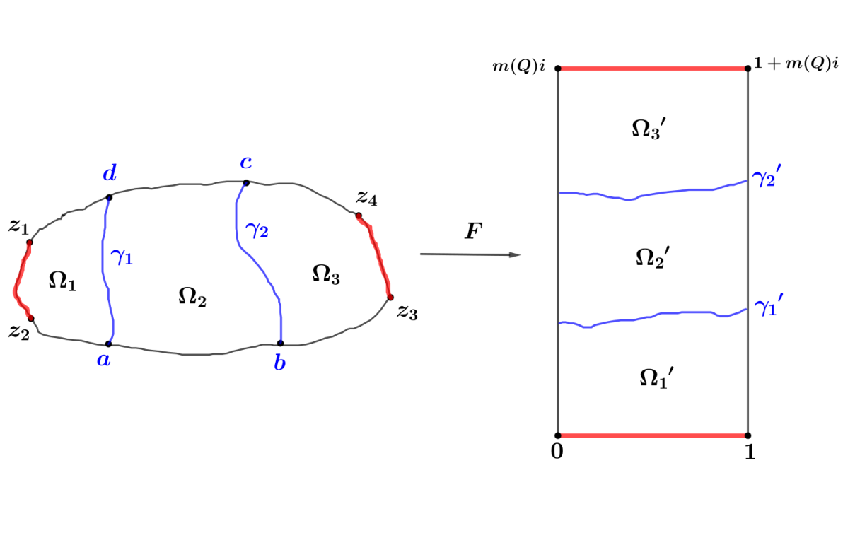
Let $\Omega$ be a Jordan domain in $\mathbb{C}$ and consinder a system consisting of $\Omega$ and four distinct points $z_{1},z_{2},z_{3},z_{4}$ in counterclockwise order on its boundary $\partial\Omega$ . Such a system is said to be a quadrilateral $Q$ and is denoted by

Q:=\left\{{\Omega;{z_{1}},{z_{2}},{z_{3}},{z_{4}}}\right\}.

The conformal module $m\left(Q\right)$ of $Q$ is the unique number for which $Q$ is conformally equivalent to the rectangular quadrilateral

Q^{\prime}:=\left\{{R_{m\left(Q\right)};0,1,1+m\left(Q\right)i,m\left(Q\right)i}\right\},

where $R_{m\left(Q\right)}=\left\{{x+yi:0<x<1,0<y<m\left(Q\right)}\right\}$ (see Fig. 3). Note that $m\left(Q\right)$ is conformally invariant and it is equal to the extremal distance between the boundary arcs $\left({z_{1}},{z_{2}}\right)$ and $\left({z_{3}},{z_{4}}\right)$ of $\Omega$ . So, $\Omega$ and $Q:=\left\{{\Omega;{z_{1}},{z_{2}},{z_{3}},{z_{4}}}\right\}$ will denote respectively the original domain and the corresponding quadrilateral. Moreover, ${\Omega_{1}},{\Omega_{2}},\ldots,$ and ${Q_{1}},{Q_{2}},\ldots,$ will denote the principle subdomains and corresponding component quadrilaterals of the decomposition under consideration. Now consider the situation of Fig. 3, where the decomposition of $Q:=\left\{{\Omega;{z_{1}},{z_{2}},{z_{3}},{z_{4}}}\right\}$ is defined by two non-intersecting arcs $\gamma_{1},\gamma_{2}$ that join respectively two distinct points $a$ and $b$ on the boundary arc $\left({{z_{2}},{z_{3}}}\right)$ to two points $d$ and $c$ on the boundary arc $\left({{z_{4}},{z_{1}}}\right)$ . These two arcs subdivide $\Omega$ into three non-intersecting subdomains denoted by ${\Omega_{1}},{\Omega_{2}}$ and ${\Omega_{3}}$ . In addition, the arc $\gamma_{1}$ subdivides $\Omega$ into $\Omega_{1}$ and another subdomain denoted by ${\Omega_{2,3}}$ , i.e. we take

{\overline{\Omega}_{2,3}}={\overline{\Omega}_{2}}\cup{\overline{\Omega}_{3}}.

Similarly, we say that $\gamma_{2}$ subdivides $\Omega$ into $\Omega_{1,2}$ and $\Omega_{3}$ , i.e. we take

{\overline{\Omega}_{1,2}}={\overline{\Omega}_{1}}\cup{\overline{\Omega}_{2}}.

Finally, we use the notations $Q_{1},Q_{2},Q_{3},Q_{1,2}$ and $Q_{2,3}$ to denote, respectively, the quadrilaterals corresponding to the subdomains $\Omega_{1},\Omega_{2},\Omega_{3},\Omega_{1,2}$ and $\Omega_{2,3}$ , i.e.

Q_{1}:=\left\{{\Omega_{1};{z_{1}},{z_{2}},a,d}\right\},\;Q_{2}:=\left\{{\Omega_{2};d,a,b,c}\right\},\;Q_{3}:=\left\{{\Omega_{3};c,b,z_{3},z_{4}}\right\}

and

Q_{1,2}:=\left\{{\Omega_{1,2};{z_{1}},{z_{2}},b,c}\right\},\;Q_{2,3}:=\left\{{\Omega_{2,3};d,a,z_{3},z_{4}}\right\}.

The following theorem was proved by Papamichael and Stylianopoulos in [15, p. 221-222]; see also [7, p. 454-455].

Theorem 2.4.

Consider the decomposition and the notations illustrated in Fig. 3. With the terminology defined above, we have

\left|{m\left(Q\right)-\left({m\left({{Q_{1,2}}}\right)+m\left({{Q_{2,3}}}\right)-m\left({{Q_{2}}}\right)}\right)}\right|\leq 8.82{e^{-\pi m\left({{Q_{2}}}\right)}},

provided that $m\left({{Q_{2}}}\right)\geq 3$ .

Remark 2.1.

Papamichael and Stylianopoulos proved Theorem 2.4 in case $\Omega$ is a Jordan domain. However, it follows from the proof that the theorem is still valid if $\Omega$ is a simply connected domain and its boundary sets $\left({{z_{1}},{z_{2}}}\right)$ and $\left({{z_{3}},{z_{4}}}\right)$ are arcs of prime ends.

2.5 Beurling’s estimates for harmonic measure

A basic property of extremal distance is its connection to harmonic measure as the following theorems, due mainly to Beurling, state (see [3, p. 280], [4, p. 369-372], [8, p. 143-146] and [11, p. 100]).

Theorem 2.5.

Let $D$ be a simply connected domain in $\mathbb{C}$ and $E$ consist of a finite number of arcs lying on $\partial D$ . Fix $z_{0}\in D$ and choose a curve $\gamma_{0}$ that contains $z_{0}$ , lies in $D$ and joins two points of $\partial D$ so that $\gamma_{0}$ bounds with $\partial D$ a domain $D_{0}$ and $z_{0}$ can be joined to $E$ inside $D\backslash{D_{0}}$ (see Fig. 4). If ${\lambda_{D\backslash{D_{0}}}}\left({{\gamma_{0}},E}\right)>2$ , then

{\omega_{D}}\left({{z_{0}},E}\right)\leq 3\pi{e^{-\pi{\lambda_{D\backslash{D_{0}}}}\left({{\gamma_{0}},E}\right)}}.

Theorem 2.6.

Let $D$ be a simply connected domain in $\mathbb{C}$ and $E$ be an arc (of prime ends) on $\partial D$ . Fix $z_{0}\in D$ and map $D$ onto $\mathbb{D}$ by the conformal map $f$ so that ${f\left({{z_{0}}}\right)=0}$ and $f\left(E\right)=\left\{{{e^{i\theta}}:\theta\in\left[{-t,t}\right]}\right\}$ for some $t\in\left[{0,\pi}\right]$ . If ${\gamma_{E}}:={f^{-1}}\left({\left[{-1,0}\right]}\right)$ , then there exists an absolute positive constant $C$ such that

{\omega_{D}}\left({{z_{0}},E}\right)\geq C{e^{-\pi{\lambda_{D}}\left({{\gamma_{E}},E}\right)}}.

3 Auxilary lemmas

Let $\Omega$ be a simply connected domain of the form illustrated in Fig. 5. Note that the positive numbers ${\alpha_{0}},{\alpha_{1}},{\alpha_{2}},\ldots,$ are the real parts of the tips of the horizontal boundary segments of $\Omega$ . We consider the straight line crosscuts $l_{1},l$ of Fig. 5 so that $l$ lies on the vertical line passing through the midpoint of $\left[{{\alpha_{0}},{\alpha_{1}}}\right]$ and $l_{1}$ lies on the vertical line passing through the midpoint of $\left[{{\alpha_{0}},\frac{{{\alpha_{0}}+{\alpha_{1}}}}{2}}\right]$ . We decompose $\Omega$ by means of the straight line crosscuts $l_{1},l,{l_{1}}^{\prime}$ into four subdomains $\Omega_{1},\Omega_{2},\Omega_{3},\Omega_{4}$ so that $\Omega_{3}$ is the reflection of $\Omega_{2}$ in $l$ .

Lemma 3.1.

With the notation above, let $Q=\left\{{\Omega;{z_{1}},0,{z_{2}},{z_{3}}}\right\}$ . According to the terminology introduced in Section 2, we have for the decomposition defined by $l$ ,

0\leq m\left(Q\right)-\left({m\left({{Q_{1,2}}}\right)+m\left({{Q_{3,4}}}\right)}\right)\leq 26.46{e^{-\pi m\left({{Q_{2}}}\right)}},

provided that $m\left({{Q_{2}}}\right)\geq 3$ .

Proof.

Since $\left[{{z_{1}},0}\right]$ and $\left[{{z_{2}},{z_{3}}}\right]$ are arcs of prime ends, there exists a conformal map $F$ of $Q$ onto $F\left(Q\right)=\left\{{{R_{m\left(Q\right)}};0,1,1+m\left(Q\right)i,m\left(Q\right)i}\right\}$ , where ${R_{m\left(Q\right)}}=\left\{{x+yi:0<x<1,0<y<m\left(Q\right)}\right\}$ . By symmetry we have that ${m\left({{Q_{2,3}}}\right)=2m\left({{Q_{2}}}\right)\geq 6}$ . So, applying Theorem 2.4 we get

\left|{m\left(Q\right)-\left({m\left({{Q_{1,2,3}}}\right)+m\left({{Q_{2,3,4}}}\right)-m\left({{Q_{2,3}}}\right)}\right)}\right|\leq 8.82{e^{-\pi m\left({{Q_{2,3}}}\right)}}

or equivalently

(3.1)

\left|{m\left(Q\right)-\left({m\left({{Q_{1,2,3}}}\right)+m\left({{Q_{2,3,4}}}\right)-2m\left({{Q_{2}}}\right)}\right)}\right|\leq 8.82{e^{-2\pi m\left({{Q_{2}}}\right)}}.

Now consider the quadrilateral $Q_{2,3,4}$ . Since $m\left({{Q_{3}}}\right)=m\left({{Q_{2}}}\right)\geq 3$ , by applying Theorem 2.4, we deduce that

\left|{m\left(Q_{2,3,4}\right)-\left({m\left({{Q_{2,3}}}\right)+m\left({{Q_{3,4}}}\right)-m\left({{Q_{3}}}\right)}\right)}\right|\leq 8.82{e^{-\pi m\left({{Q_{3}}}\right)}}

or equivalently

(3.2)

\left|{m\left(Q_{2,3,4}\right)-\left({m\left({{Q_{2}}}\right)+m\left({{Q_{3,4}}}\right)}\right)}\right|\leq 8.82{e^{-\pi m\left({{Q_{2}}}\right)}}.

Similarly, consider the quadrilateral $Q_{1,2,3}$ . Since $m\left({{Q_{2}}}\right)\geq 3$ , by applying Theorem 2.4, we deduce that

\left|{m\left(Q_{1,2,3}\right)-\left({m\left({{Q_{1,2}}}\right)+m\left({{Q_{2,3}}}\right)-m\left({{Q_{2}}}\right)}\right)}\right|\leq 8.82{e^{-\pi m\left({{Q_{2}}}\right)}}

or equivalently

(3.3)

\left|{m\left(Q_{1,2,3}\right)-\left({m\left({{Q_{2}}}\right)+m\left({{Q_{1,2}}}\right)}\right)}\right|\leq 8.82{e^{-\pi m\left({{Q_{2}}}\right)}}.

By relations (3.1), (3.2), (3.3) and the serial rule

{m\left(Q\right)\geq m\left({{Q_{1,2}}}\right)+m\left({{Q_{3,4}}}\right)},

we finally get

0\leq m\left(Q\right)-\left({m\left({{Q_{1,2}}}\right)+m\left({{Q_{3,4}}}\right)}\right)\leq 26.46{e^{-\pi m\left({{Q_{2}}}\right)}}.

∎

In the following lemma we use the notation $D\left({0,\alpha}\right)$ to denote the disk with center at 0 and radius $\alpha$ .

Lemma 3.2.

Let $\Omega$ be a simply connected domain of the form illustrated in Fig. 6 and $E$ be an arc of prime ends on $\partial\Omega\cap\partial D\left({0,\alpha}\right)$ . If $f$ is the conformal map of $\Omega$ onto $\mathbb{D}$ such that $f\left(0\right)=0$ and $f\left(E\right)=\left\{{{e^{i\theta}}:\theta\in\left[{-t,t}\right]}\right\}$ for some ${t\in\left[{0,\pi}\right]}$ , then

\gamma\subset\overline{D}\left({0,\alpha_{0}}\right),

where $\gamma:={f^{-1}}\left({\left[{-1,0}\right]}\right)$ .

Proof.

Set $C=\left\{{\alpha_{0}{e^{i\theta}}:\theta\in\left[{\frac{\pi}{2},2\pi}\right]}\right\}$ and ${z_{0}}={f^{-1}}\left({-1}\right)$ . Since $D\left({0,\alpha_{0}}\right)\subset\Omega$ , by Corollary 4.3.9 [19, p. 102] and conformal invariance of harmonic measure, we have

{\omega_{\mathbb{D}}}\left({0,f\left(C\right)}\right)={\omega_{\Omega}}\left({0,C}\right)\geq{\omega_{D\left({0,\alpha_{0}}\right)}}\left({0,C}\right)=\frac{3}{4}.

This, in conjunction with the fact that $f\left(C\right)\cap f\left(E\right)=\emptyset$ and $f\left(C\right)$ is a connected arc of $\partial\mathbb{D}$ , implies that

\left\{{{e^{i\theta}}:\theta\in\left[{\frac{\pi}{2},\frac{{3\pi}}{2}}\right]}\right\}\subset f\left(C\right).

So, ${z_{0}}={f^{-1}}\left({-1}\right)\in C$ . Now suppose that $\gamma\not\subset\overline{D}\left({0,\alpha_{0}}\right)$ . Then $\gamma$ contains a curve $\gamma_{0}$ lying in $\Omega\backslash D\left({0,\alpha_{0}}\right)$ with endpoints $z_{1},z_{2}\in\partial{D\left({0,\alpha_{0}}\right)}$ (see Fig. 8, 8).

Since $\gamma$ is the hyperbolic geodesic joining $0$ to ${z_{0}}$ in $\Omega$ , $\gamma_{0}$ is the hyperbolic geodesic joining $z_{1}$ to ${z_{2}}$ in $\Omega$ . Notice that $\Omega$ is a hyperbolic region in $\mathbb{C}$ such that $\Omega\cap\partial D\left({0,\alpha_{0}}\right)\neq\emptyset$ and $\Omega\backslash D\left({0,\alpha_{0}}\right)\subset\Omega^{*}$ , where $\Omega^{*}$ is the reflection of $\Omega$ in the circle $\partial D\left({0,\alpha_{0}}\right)$ . So, applying Theorem 2.1 we get

{\lambda_{{\Omega^{*}}}}\left(z\right)<{\lambda_{\Omega}}\left(z\right),\;z\in{\gamma_{0}}

and thus

\int_{{\gamma_{0}}^{*}}{{\lambda_{\Omega}}\left({{z^{*}}}\right)\left|{d{z^{*}}}\right|}<\int_{{\gamma_{0}}}{{\lambda_{\Omega}}\left(z\right)\left|{dz}\right|},

where ${\gamma_{0}}^{*}$ is the reflection of $\gamma_{0}$ in $\partial D\left({0,\alpha_{0}}\right)$ . But this leads to contradiction because $\gamma_{0}$ is the hyperbolic geodesic joining $z_{1}$ to ${z_{2}}$ in $\Omega$ . So, $\gamma\subset\overline{D}\left({0,\alpha_{0}}\right)$ . Note that the same result could come from Jørgensen’ s theorem that closed disks in $\Omega$ are strictly convex in the hyperbolic geometry of $\Omega$ (see [20]).

∎

Lemma 3.3.

Let $\Omega,\gamma,E$ be as in Lemma 3.2 and ${z_{1}},{z_{2}},{z_{3}}$ be the points illustrated in Fig. 9. Take $r_{1},r_{2}$ so that $\alpha_{0}<{r_{1}}<{r_{2}}<{\alpha_{1}}$ and $\log\frac{{{r_{2}}}}{{{r_{1}}}}\geq\frac{{3\pi}}{2}$ . Decomposing $Q=\left\{{{\Omega\backslash\gamma};{z_{1}},{z_{1}},{z_{2}},{z_{3}}}\right\}$ as in Fig. 9, with the terminology introduced in Section 2, we have

\left|{m\left(Q\right)-\left({m\left({{Q_{1,2}}}\right)+m\left({{Q_{2,3}}}\right)-m\left({{Q_{2}}}\right)}\right)}\right|\leq 8.82{e^{-\pi m\left({{Q_{2}}}\right)}}.

In the notation $Q=\left\{{{\Omega\backslash\gamma};{z_{1}},{z_{1}},{z_{2}},{z_{3}}}\right\}$ , by the pair of points ${z_{1}},{z_{1}}$ , we mean the two different prime ends supported at the point ${z_{1}}$ .

Proof.

First, applying the conformal map $f\left(z\right)=\LOG z$ (principal branch of the logarithm) on the quadrilateral ${Q_{2}}=\left\{{{\Omega_{2}};{r_{1}}i,{r_{1}},{r_{2}},{r_{2}}i}\right\}$ we take the rectangular quadrilateral

f\left({{Q_{2}}}\right)=\left\{{f\left({{\Omega_{2}}}\right);\log{r_{1}}+\frac{\pi}{2}i,\log{r_{1}},\log{r_{2}},\log{r_{2}}+\frac{\pi}{2}i}\right\},

where $f\left({{\Omega_{2}}}\right)=\left\{{x+yi:\log{r_{1}}<x<\log{r_{2}},0<y<{\pi\mathord{\left/{\vphantom{\pi 2}}\right.\kern-1.2pt}2}}\right\}$ . Because of the conformal invariance of modules and our assumption about $r_{1},r_{2}$ ,

m\left({{Q_{2}}}\right)=m\left(f\left({{Q_{2}}}\right)\right)=\frac{{\log\left({{{{r_{2}}}\mathord{\left/{\vphantom{{{r_{2}}}{{r_{1}}}}}\right.\kern-1.2pt}{{r_{1}}}}}\right)}}{{{\pi\mathord{\left/{\vphantom{\pi 2}}\right.\kern-1.2pt}2}}}\geq 3.

Since the boundary sets $\left({{z_{1}},0,{z_{1}}}\right)$ and $E$ are arcs of prime ends, there exists a conformal map $F$ of $Q$ onto

Q^{\prime}=\left\{{R_{m\left(Q\right)};0,1,1+m\left(Q\right)i,m\left(Q\right)i}\right\},

where $R_{m\left(Q\right)}=\left\{{x+yi:0<x<1,0<y<m\left(Q\right)}\right\}$ . Since $m\left({{Q_{2}}}\right)\geq 3$ , Theorem 2.4 implies that

\left|{m\left(Q\right)-\left({m\left({{Q_{1,2}}}\right)+m\left({{Q_{2,3}}}\right)-m\left({{Q_{2}}}\right)}\right)}\right|\leq 8.82{e^{-\pi m\left({{Q_{2}}}\right)}}.

∎

4 The first example

Theorem 4.1.

There exists an unbounded simply connected domain $D$ with the following properties: Let $\psi$ be a conformal map of $\mathbb{D}$ onto $D$ with $\psi\left(0\right)=0$ . If ${F_{\alpha}}=\left\{{z\in\mathbb{D}:\left|{\psi\left(z\right)}\right|=\alpha}\right\}$ for $\alpha>0$ , then

(1)

the number of components of $\psi\left({F_{\alpha}}\right)$ tends to infinity as $\alpha\to+\infty$ and
(2)

$\forall K>0$ $\exists\alpha$ such that

${\omega_{\mathbb{D}}}\left({0,{F_{\alpha}}}\right)\geq K{e^{-{d_{\mathbb{D}}}\left({0,{F_{\alpha}}}\right)}}.$

Proof.

Step 1: If $\alpha_{0}=1,\;\alpha_{1}={e^{4\pi}},\;\alpha_{2}={e^{8\pi}},\ldots,\alpha_{n}={e^{4n\pi}},\ldots$ , let $D$ be the simply connected domain of Fig. 10, namely

D=\mathbb{C}\backslash\bigcup\limits_{k=0}^{3}{\left[{{\alpha_{0}}{e^{i\frac{{k\pi}}{2}}},+\infty}\right)}\backslash\bigcup\limits_{l=1}^{+\infty}{\bigcup\limits_{k=0}^{{2^{l+1}}-1}{\left[{{\alpha_{l}}{e^{i\frac{\pi}{{{2^{l}}}}\left({\frac{1}{2}+k}\right)}},+\infty}\right)}},

with the notation $\left[{r{e^{i\theta}},+\infty}\right)=\left\{{s{e^{i\theta}}:s\geq r}\right\}$ .

The Riemann Mapping Theorem implies that there exists a conformal map $\psi$ from $\mathbb{D}$ onto $D$ such that $\psi\left(0\right)=0$ . Let $N\left(\alpha\right)$ be the number of components of $\psi\left({{F_{\alpha}}}\right)=D\cap\partial D\left({0,\alpha}\right)$ , then we have

N\left(\alpha\right)=\left\{\begin{array}[]{l}1,\;\;\;\;\;\;\;if\;\alpha\in\left({0,{\alpha_{0}}}\right)\\ {2^{2}},\;\;\;\;\;if\;\alpha\in\left[{{\alpha_{0}},{\alpha_{1}}}\right)\\ {2^{3}},\;\;\;\;\;if\;\alpha\in\left[{{\alpha_{1}},{\alpha_{2}}}\right)\\ \vdots\\ {2^{n+2}},\;if\;\alpha\in\left[{{\alpha_{n}},{\alpha_{n+1}}}\right)\\ \vdots\end{array}\right.

Step 2: We fix a real number $\alpha$ such that $\alpha>{\alpha_{1}}$ and $\alpha\neq{\alpha_{n}}$ for every $n\in\mathbb{N}$ . Then there exists a fixed number $n\in\mathbb{N}$ such that $\alpha\in\left({{\alpha_{n}},{\alpha_{n+1}}}\right)$ and thus $N\left(\alpha\right)={2^{n+2}}$ . Since hyperbolic distance is conformally invariant we have

(4.1)

{e^{-{d_{\mathbb{D}}}\left({0,{F_{\alpha}}}\right)}}={e^{-{d_{D}}\left({0,\psi\left({{F_{\alpha}}}\right)}\right)}}={e^{-{d_{D}}\left({0,{\psi\left({F_{\alpha}^{*}}\right)}}\right)}},

where ${\psi\left({F_{\alpha}^{*}}\right)}$ is a component of $\psi\left({{F_{\alpha}}}\right)$ containing a point $z_{0}$ for which

{d_{D}}\left({0,\psi\left({{F_{\alpha}}}\right)}\right)=\inf\left\{{{d_{D}}\left({0,z}\right):z\in\psi\left({{F_{\alpha}}}\right)}\right\}={d_{D}}\left({0,{z_{0}}}\right).

Due to the symmetry of $D$ , we may assume without loss of generality that ${\psi\left({F_{\alpha}^{*}}\right)}$ lies on the first quartile $P=\left\{{z\in\mathbb{C}:\IM z>0,\;\RE z>0}\right\}$ . By relation (1.2) of Section 1, we infer that

{e^{-{d_{\mathbb{D}}}\left({0,{F_{\alpha}^{*}}}\right)}}\leq\frac{\pi}{2}{\omega_{\mathbb{D}}}\left({0,{F_{\alpha}^{*}}}\right)

which in conjunction with the conformal invariance gives

(4.2)

{e^{-{d_{D}}\left({0,{\psi\left({F_{\alpha}^{*}}\right)}}\right)}}\leq\frac{\pi}{2}{\omega_{D}}\left({0,{\psi\left({F_{\alpha}^{*}}\right)}}\right).

Moreover, by Theorem 2.5 we deduce that

(4.3)

{\omega_{D}}\left({0,{\psi\left({F_{\alpha}^{*}}\right)}}\right)\leq 3\pi{e^{-\pi{\lambda_{D^{\prime}}}\left({\gamma,{\psi\left({F_{\alpha}^{*}}\right)}}\right)}},

where $\gamma$ is the arc of the circle passing through the points $0,\;1,\;i$ such that $\gamma$ connects $i$ to $1$ and $\gamma\cap P=\emptyset$ and $D^{\prime}$ is the subdomain of $D$ bounded by $\gamma$ , $\left[{1,\alpha}\right],\;\left[{i,\alpha i}\right],\;P\cap\partial D\left({0,\alpha}\right)$ and $\partial D\cap P\cap D\left({0,\alpha}\right)$ (see Fig. 12). If $\gamma_{0}=\partial\mathbb{D}\cap\overline{P}$ and $D^{\prime\prime}$ is the subdomain of $D^{\prime}$ bounded by $\gamma_{0}$ , $\left[{1,\alpha}\right],\;\left[{i,\alpha i}\right]\;P\cap\partial D\left({0,\alpha}\right)$ and $\partial D\cap P\cap D\left({0,\alpha}\right)$ (see Fig. 12), then by Theorem 2.2 we have

(4.4)

{\lambda_{D^{\prime}}}\left({\gamma,{\psi\left({F_{\alpha}^{*}}\right)}}\right)\geq{\lambda_{D^{\prime\prime}}}\left({{\gamma_{0}},{\psi\left({F_{\alpha}^{*}}\right)}}\right).

Combining the relations (4.1), (4.2), (4.3) and (4.4), we obtain

(4.5)

{e^{-{d_{\mathbb{D}}}\left({0,{F_{\alpha}}}\right)}}\leq\frac{{3{\pi^{2}}}}{2}{e^{-\pi{\lambda_{D^{\prime\prime}}}\left({{\gamma_{0}},{\psi\left({F_{\alpha}^{*}}\right)}}\right)}}.

Next we consider the crosscuts ${\gamma_{1}},{\gamma_{2}},{\gamma_{3}},\ldots,{\gamma_{n-1}}$ of $D^{\prime\prime}$ , where for $j=1,2,3,\ldots,n-1$ , $\gamma_{j}$ is an arc of the circle with center at $0$ and radius equal to the midpoint of ${\left[{{\alpha_{j}},{\alpha_{j+1}}}\right]}$ as illustrated in Fig. 13.

Setting

m\left({{Q_{1}}}\right):={\lambda_{D^{\prime\prime}}}\left({{\gamma_{0}},{\gamma_{1}}}\right),\;m\left({{Q_{2}}}\right):={\lambda_{D^{\prime\prime}}}\left({{\gamma_{1}},{\gamma_{2}}}\right),\ldots,\;m\left({{Q_{n}}}\right):={\lambda_{D^{\prime\prime}}}\left({{\gamma_{n-1}},{\psi\left({F_{\alpha}^{*}}\right)}}\right),

by the serial rule we deduce that

(4.6)

{\lambda_{D^{\prime\prime}}}\left({{\gamma_{0}},{\psi\left({F_{\alpha}^{*}}\right)}}\right)\geq m\left({{Q_{1}}}\right)+m\left({{Q_{2}}}\right)+\ldots+m\left({{Q_{n}}}\right)

and thus by (4.5) and (4.6),

(4.7)

{e^{-{d_{\mathbb{D}}}\left({0,{F_{\alpha}}}\right)}}\leq\frac{{3{\pi^{2}}}}{2}{e^{-\pi\left({m\left({{Q_{1}}}\right)+m\left({{Q_{2}}}\right)+\ldots+m\left({{Q_{n}}}\right)}\right)}}.

Step 3: Since harmonic measure is conformally invariant and $N\left(\alpha\right)={2^{n+2}}$ , we have

{\omega_{\mathbb{D}}}\left({0,{F_{\alpha}}}\right)={\omega_{D}}\left({0,\psi\left({{F_{\alpha}}}\right)}\right)=\sum\limits_{j=1}^{N\left(\alpha\right)}{{\omega_{D}}\left({0,\psi{{\left({{F_{\alpha}}}\right)}^{j}}}\right)}\geq N\left(\alpha\right){\omega_{D}}\left({0,\psi{{\left({{F_{\alpha}}}\right)}^{m}}}\right)={2^{n+2}}{\omega_{D}}\left({0,\psi{{\left({{F_{\alpha}}}\right)}^{m}}}\right),

where ${\psi{{\left({{F_{\alpha}}}\right)}^{j}}}$ , $j=1,2,3,\ldots,N(\alpha)$ , are the components of ${\psi{{\left({{F_{\alpha}}}\right)}}}$ and

{\omega_{D}}\left({0,\psi{{\left({{F_{\alpha}}}\right)}^{m}}}\right)=\min\left\{{{\omega_{D}}\left({0,\psi{{\left({{F_{\alpha}}}\right)}^{j}}}\right):j\in\left\{{1,2,3,\ldots,N(\alpha)}\right\}}\right\}.

If $D^{*}$ is the subdomain of $D$ bounded by $\left[{\frac{1}{2},\alpha}\right],\;\left[{\frac{1}{2}i,\alpha i}\right],\;\partial D\left({0,\frac{1}{2}}\right)\backslash P,\;\partial D\left({0,\alpha}\right)\cap P$ and $\partial D\cap D\left({0,\alpha}\right)\cap P$ as illustrated in Fig. 14, then applying Corollary 4.3.9 [19, p. 102] we obtain

{\omega_{D}}\left({0,\psi{{\left({{F_{\alpha}}}\right)}^{m}}}\right)\geq{\omega_{{D^{*}}}}\left({0,\psi{{\left({{F_{\alpha}}}\right)}^{m}}}\right)

and hence

(4.8)

{\omega_{\mathbb{D}}}\left({0,{F_{\alpha}}}\right)\geq{2^{n+2}}{\omega_{{D^{*}}}}\left({0,\psi{{\left({{F_{\alpha}}}\right)}^{m}}}\right).

Step 4: If $h_{m}$ is the conformal map of $D^{*}$ onto $\mathbb{D}$ such that ${h_{m}}\left(0\right)=0$ and ${h_{m}}\left({\psi{{\left({{F_{\alpha}}}\right)}^{m}}}\right)=\left\{{{e^{i\theta}}:\theta\in\left[{-t,t}\right]}\right\}$ for some $t\in\left[{0,\pi}\right]$ and ${\gamma_{m}}:=h_{m}^{-1}\left({\left[{-1,0}\right]}\right)$ , then by Theorem 2.6 there exists a positive constant $C_{0}$ such that

(4.9)

{\omega_{{D^{*}}}}\left({0,\psi{{\left({{F_{\alpha}}}\right)}^{m}}}\right)\geq{C_{0}}{e^{-\pi{\lambda_{{D^{*}}}}\left({{\gamma_{m}},\psi{{\left({{F_{\alpha}}}\right)}^{m}}}\right)}}.

Furthermore, by Lemma 3.2 we infer that ${\gamma_{m}}\subset\overline{D}\left({0,\frac{1}{2}}\right)$ . So, taking the crosscuts ${\gamma_{0}}=\overline{{D^{*}}}\cap\partial\mathbb{D}$ and ${\gamma_{0}}^{\prime}=\overline{{D^{*}}}\cap\partial D\left({0,{e^{{{3\pi}\mathord{\left/{\vphantom{{3\pi}2}}\right.\kern-1.2pt}2}}}}\right)$ of $D^{*}$ (see Fig. 16, 16) and applying Lemma 3.3 we obtain

(4.10)

{\lambda_{{D^{*}}}}\left({{\gamma_{m}},\psi{{\left({{F_{\alpha}}}\right)}^{m}}}\right)\leq 8.82{e^{-3\pi}}-3+{\lambda_{{D^{*}}}}\left({{\gamma_{m}},{\gamma_{0}}^{\prime}}\right)+{\lambda_{{D^{*}}}}\left({{\gamma_{0}},\psi{{\left({{F_{\alpha}}}\right)}^{m}}}\right).

where ${\lambda_{{D^{*}}}}\left({{\gamma_{0}},{\gamma_{0}}^{\prime}}\right)=3$ and ${\lambda_{{D^{*}}}}\left({{\gamma_{m}},{\gamma_{0}}^{\prime}}\right)$ is bounded from above by a positive constant $C_{1}$ for every $\alpha>0$ and every $m$ (see [4, p. 370-371] for a similar estimate). By relations (4.8), (4.9) and (4.10), we get

(4.11)

{\omega_{\mathbb{D}}}\left({0,{F_{\alpha}}}\right)\geq{2^{n+2}}{C_{0}}{e^{\left({3-8.82{e^{-3\pi}}}\right)\pi}}{e^{-{C_{1}}\pi}}{e^{-\pi{\lambda_{{D^{*}}}}\left({{\gamma_{0}},\psi{{\left({{F_{\alpha}}}\right)}^{m}}}\right)}}.

Step 5: Now we concentrate on ${e^{-\pi{\lambda_{{{D^{*}}}}}\left({{\gamma_{0}},\psi{{\left({{F_{\alpha}}}\right)}^{m}}}\right)}}$ or equivalently on ${e^{-\pi{\lambda_{D^{\prime\prime}}}\left({{\gamma_{0}},\psi{{\left({{F_{\alpha}}}\right)}^{m}}}\right)}}$ . First we take the crosscuts $\gamma_{1}^{m},\gamma_{2}^{m},\gamma_{3}^{m},\ldots,\gamma_{n-1}^{m}$ of $D^{\prime\prime}$ , where, for $j=1,2,3,\ldots,n-1$ , $\gamma_{j}^{m}$ is an arc of the circle with center at $0$ and radius equal to the midpoint of ${\left[{{\alpha_{j}},{\alpha_{j+1}}}\right]}$ as illustrated in Fig. 17, and set

m\left({{Q_{1}^{m}}}\right):={\lambda_{D^{\prime\prime}}}\left({{\gamma_{0}},{\gamma_{1}^{m}}}\right),\;m\left({{Q_{2}^{m}}}\right):={\lambda_{D^{\prime\prime}}}\left({{\gamma_{1}^{m}},{\gamma_{2}^{m}}}\right),\ldots,\;m\left({{Q_{n}^{m}}}\right):={\lambda_{D^{\prime\prime}}}\left({{\gamma_{n-1}^{m}},{\psi\left({F_{\alpha}}\right)^{m}}}\right).

Applying the conformal map $f\left(z\right)=\LOG z$ on $D^{\prime\prime}$ we take $f\left({D^{\prime\prime}}\right),f\left({{\gamma_{0}}}\right),f\left({\psi{{\left({{F_{\alpha}}}\right)}^{m}}}\right)$ and $f\left({\gamma_{1}^{m}}\right),\ldots,f\left({\gamma_{n-1}^{m}}\right),f\left({Q_{1}^{m}}\right),\ldots,f\left({Q_{n}^{m}}\right)$ illustrated in Fig. 18. The conformal invariance of extremal length implies that for every $j=1,2,3,\ldots,n$ ,

{\lambda_{D^{\prime\prime}}}\left({{\gamma_{0}},\psi{{\left({{F_{\alpha}}}\right)}^{m}}}\right)={\lambda_{f\left({D^{\prime\prime}}\right)}}\left({f\left({{\gamma_{0}}}\right),f\left({\psi{{\left({{F_{\alpha}}}\right)}^{m}}}\right)}\right),\;m\left({Q_{j}^{m}}\right)=m\left({f\left({Q_{j}^{m}}\right)}\right).

This leads us to consider the crosscuts ${l_{1}},{l_{1}}^{\prime},{l_{2}},{l_{2}}^{\prime},\ldots,{l_{n-1}},{l_{n-1}}^{\prime}$ of $f\left({D^{\prime\prime}}\right)$ so that, for $j=1,2,\ldots,n-1$ , each of $l_{j}$ is a segment which lies on a vertical line passing through the midpoint of $\left[{f\left({{\alpha_{j}}}\right),\frac{{f\left({{\alpha_{j}}}\right)+f\left({{\alpha_{j+1}}}\right)}}{2}}\right]=\left[{4j\pi,2\left({2j+1}\right)\pi}\right]$ and ${l_{j}}^{\prime}$ is the reflection of $l_{j}$ in $f\left({\gamma_{j}^{m}}\right)$ (see Fig. 18). Now let $R_{j}$ be the rectangle formed by ${\partial f\left({D^{\prime\prime}}\right)}$ and ${l_{j}},f\left({\gamma_{j}^{m}}\right)$ for $j=1,2,3,\ldots,n-1$ as illustrated in Fig 18. Since

$\displaystyle m\left({{R_{1}}}\right)$	$\displaystyle=$	$\displaystyle\frac{{{\pi}}}{{{\pi\mathord{\left/{\vphantom{\pi 4}}\right.\kern-1.2pt}4}}}={2^{2}}>3$
$\displaystyle m\left({{R_{2}}}\right)$	$\displaystyle=$	$\displaystyle\frac{{{\pi}}}{{{\pi\mathord{\left/{\vphantom{\pi 8}}\right.\kern-1.2pt}8}}}={2^{3}}$
$\displaystyle m\left({{R_{n-1}}}\right)$	$\displaystyle=$	$\displaystyle\frac{{{\pi}}}{{{\pi\mathord{\left/{\vphantom{\pi{{2^{n}}}}}\right.\kern-1.2pt}{{2^{n}}}}}}={2^{n}},$

we can apply Lemma 3.1 successively and obtain

$\displaystyle 0\leq{\lambda_{D^{\prime\prime}}}\left({{\gamma_{0}},\psi{{\left({{F_{\alpha}}}\right)}^{m}}}\right)-\left({m\left({Q_{1}^{m}}\right)+m\left({{{\left({Q_{1}^{m}}\right)}^{c}}}\right)}\right)$	$\displaystyle\leq$	$\displaystyle 26.46{e^{-\pi m\left({{R_{1}}}\right)}}$
$\displaystyle 0\leq m\left({{{\left({Q_{1}^{m}}\right)}^{c}}}\right)-\left({m\left({Q_{2}^{m}}\right)+m\left({{{\left({Q_{2}^{m}}\right)}^{c}}}\right)}\right)$	$\displaystyle\leq$	$\displaystyle 26.46{e^{-\pi m\left({{R_{2}}}\right)}}$
$\displaystyle 0\leq m\left({{{\left({Q_{n-2}^{m}}\right)}^{c}}}\right)-\left({m\left({Q_{n-1}^{m}}\right)+m\left({{{\left({Q_{n-1}^{m}}\right)}^{c}}}\right)}\right)$	$\displaystyle\leq$	$\displaystyle 26.46{e^{-\pi m\left({{R_{n-1}}}\right)}},$

where ${m\left({{{\left({Q_{j}^{m}}\right)}^{c}}}\right)}$ denotes the extremal length between $\gamma_{j}^{m}$ and $\psi{\left({{F_{\alpha}}}\right)^{m}}$ in $D^{\prime\prime}$ for every $j=1,2,\ldots,n-1$ and thus ${m\left({{{\left({Q_{n-1}^{m}}\right)}^{c}}}\right)=m\left({Q_{n}^{m}}\right)}$ . Adding the inequalites above, we deduce that

0\leq{\lambda_{D^{\prime\prime}}}\left({{\gamma_{0}},\psi{{\left({{F_{\alpha}}}\right)}^{m}}}\right)\leq 26.46\sum\limits_{j=1}^{n-1}{{e^{-\pi m\left({{R_{j}}}\right)}}}+m\left({Q_{1}^{m}}\right)+m\left({Q_{2}^{m}}\right)+\ldots+m\left({Q_{n}^{m}}\right),

where $m\left({{R_{j}}}\right)={2^{j+1}}$ . So,

{e^{-\pi{\lambda_{D^{\prime\prime}}}\left({{\gamma_{0}},\psi{{\left({{F_{\alpha}}}\right)}^{m}}}\right)}}\geq{e^{-26.46\pi\sum\limits_{j=1}^{n-1}{{e^{-{2^{j+1}}\pi}}}}}{e^{-\pi\left({m\left({Q_{1}^{m}}\right)+m\left({Q_{2}^{m}}\right)+\ldots+m\left({Q_{n}^{m}}\right)}\right)}}.

Since the series ${\sum\limits_{j=1}^{+\infty}{{e^{-{2^{j+1}}\pi}}}}$ converges to a positive real number $l$ , we obtain

{e^{-\pi{\lambda_{D^{\prime\prime}}}\left({{\gamma_{0}},\psi{{\left({{F_{\alpha}}}\right)}^{m}}}\right)}}\geq{C_{2}}{e^{-\pi\left({m\left({Q_{1}^{m}}\right)+m\left({Q_{2}^{m}}\right)+\ldots+m\left({Q_{n}^{m}}\right)}\right)}},

where $C_{2}:={e^{-26.46\pi l}}$ . But due to the symmetry of $D$ , we notice that the sum

m\left({Q_{1}^{m}}\right)+m\left({Q_{2}^{m}}\right)+\ldots+m\left({Q_{n}^{m}}\right)

is independent of $m$ and thus

m\left({Q_{1}^{m}}\right)+m\left({Q_{2}^{m}}\right)+\ldots+m\left({Q_{n}^{m}}\right)=m\left({{Q_{1}}}\right)+m\left({{Q_{2}}}\right)+\ldots+m\left({{Q_{n}}}\right).

This leads us to the relation

(4.12)

{e^{-\pi{\lambda_{D^{\prime\prime}}}\left({{\gamma_{0}},\psi{{\left({{F_{\alpha}}}\right)}^{m}}}\right)}}\geq{C_{2}}{e^{-\pi\left({m\left({{Q_{1}}}\right)+m\left({{Q_{2}}}\right)+\ldots+m\left({{Q_{n}}}\right)}\right)}}.

Combining the relations (4.11) and (4.12) we finally obtain

(4.13)

{\omega_{\mathbb{D}}}\left({0,{F_{\alpha}}}\right)\geq{2^{n+2}}{C_{0}}{C_{2}}{e^{\left({3-8.82{e^{-3\pi}}}\right)\pi}}{e^{-{C_{1}}\pi}}{e^{-\pi\left({m\left({{Q_{1}}}\right)+m\left({{Q_{2}}}\right)+\ldots+m\left({{Q_{n}}}\right)}\right)}}.

Step 6: Now suppose there exists a positive constant $K$ such that for every $\alpha>0$ ,

(4.14)

{\omega_{\mathbb{D}}}\left({0,{F_{\alpha}}}\right)\leq K{e^{-{d_{\mathbb{D}}}\left({0,{F_{\alpha}}}\right)}}.

Setting

{C_{3}}:=\frac{{3{\pi^{2}}}}{2}\frac{K}{{{{C_{0}}{C_{2}}}}}{e^{{C_{1}}\pi}}{e^{-\left({3-8.82{e^{-3\pi}}}\right)\pi}}

and using (4.7), (4.13) and (4.14), we infer that

{2^{n+2}}{e^{-\pi\left({m\left({{Q_{1}}}\right)+m\left({{Q_{2}}}\right)+\ldots+m\left({{Q_{n}}}\right)}\right)}}\leq{C_{3}}{e^{-\pi\left({m\left({{Q_{1}}}\right)+m\left({{Q_{2}}}\right)+\ldots+m\left({{Q_{n}}}\right)}\right)}}

or equivalently

(4.15)

{2^{n+2}}\leq{C_{3}}

for every $n\in\mathbb{N}$ . Finally, taking limits in (4.15) as $n\to+\infty$ , that is $\alpha\to+\infty$ , we obtain the contradiction

\mathop{\lim}\limits_{n\to+\infty}{2^{n+2}}\leq{C_{3}}<+\infty.

So, $\forall K>0$ $\exists\alpha$ such that

{\omega_{\mathbb{D}}}\left({0,{F_{\alpha}}}\right)\geq K{e^{-{d_{\mathbb{D}}}\left({0,{F_{\alpha}}}\right)}}.

∎

5 The second example

The main feature of $D$ which plays a central role in the proof of Theorem 4.1 is that as $\alpha\to+\infty$ , the number of components of $\psi\left({{F_{\alpha}}}\right)$ tends to infinity. Next we prove that even if the number of components of $\psi\left({{F_{\alpha}}}\right)$ is bounded from above by a positive constant for every $\alpha>0$ , the answer to the Question 1.1 is still negative. To verify this, we need the following lemma whose proof is straightforward and thus is omitted.

Lemma 5.1.

Let $\Gamma$ be the geodesic between two points $z_{1},z_{2}\in\partial{\mathbb{D}}$ in $\mathbb{D}$ . Then

{e^{-{d_{\mathbb{D}}}\left({0,\Gamma}\right)}}\leq{\omega_{\mathbb{D}}}\left({0,\Gamma}\right)\leq\frac{4}{\pi}{e^{-{d_{\mathbb{D}}}\left({0,\Gamma}\right)}}.

Theorem 5.1.

There exists an unbounded simply connected domain $D$ with the following properties: Let $\psi$ be a conformal map of $\mathbb{D}$ onto $D$ . If ${F_{\alpha}}=\left\{{z\in\mathbb{D}:\left|{\psi\left(z\right)}\right|=\alpha}\right\}$ for $\alpha>0$ , then

(1)

$\psi\left({{F_{\alpha}}}\right)$ is a connected set for every $\alpha>0$ and
(2)

$\forall K>0$ $\exists\alpha$ such that

${\omega_{\mathbb{D}}}\left({0,{F_{\alpha}}}\right)\geq K{e^{-{d_{\mathbb{D}}}\left({0,{F_{\alpha}}}\right)}}.$

Proof.

Let $D$ be the simply connected domain of Fig. 19, namely

D=\left\{{z\in\mathbb{C}\backslash\overline{\mathbb{D}}:\left|{\Arg{z}}\right|<1}\right\}\backslash\bigcup\limits_{n=1}^{+\infty}{\left\{{z\in\partial D\left({0,{e^{n}}}\right):\frac{1}{{{40^{n}}}}\leq\left|{\Arg{z}}\right|<1}\right\}}.

The Riemann Mapping Theorem implies that there exists a conformal map $\psi$ from $\mathbb{D}$ onto $D$ such that $\psi\left(0\right)={e^{\frac{1}{4}}}$ . Let ${\alpha_{n}}={e^{n-\frac{1}{{{{40}^{n}}}}}}$ for every $n\in\mathbb{N}$ and take the arcs ${\partial D\left({0,{\alpha_{n}}}\right)\cap\overline{D}}$ as illustrated in Fig. 19. Now fix a number $n>1$ . If ${\Gamma_{{\alpha_{n}}}}$ is the geodesic joining ${\psi^{-1}}\left({{\alpha_{n}}{e^{i}}}\right)$ to ${\psi^{-1}}\left({{\alpha_{n}}{e^{-i}}}\right)$ in $\mathbb{D}$ and $S_{{\alpha_{n}}}$ denotes the arc of $\partial\mathbb{D}$ between ${\psi^{-1}}\left({{\alpha_{n}}{e^{-i}}}\right)$ and ${\psi^{-1}}\left({{\alpha_{n}}{e^{i}}}\right)$ (see Fig. 20), then by Lemma 5.1 and [4, p. 370] we get

{\omega_{\mathbb{D}}}\left({0,{F_{{\alpha_{n}}}}}\right)\geq{\omega_{\mathbb{D}}}\left({0,{S_{{\alpha_{n}}}}}\right)=\frac{1}{2}{\omega_{\mathbb{D}}}\left({0,{\Gamma_{{\alpha_{n}}}}}\right)\geq\frac{1}{2}{e^{-{d_{\mathbb{D}}}\left({0,{\Gamma_{{\alpha_{n}}}}}\right)}}=\frac{1}{2}{e^{-{d_{D}}\left({{e^{\frac{1}{4}}},\psi\left({{\Gamma_{{\alpha_{n}}}}}\right)}\right)}}.

Since $\psi$ preserves the geodesics and $D$ is symmetric with respect to the real axis, we deduce that ${d_{D}}\left({{e^{\frac{1}{4}}},\psi\left({{\Gamma_{{\alpha_{n}}}}}\right)}\right)={d_{D}}\left({{e^{\frac{1}{4}}},{b_{n}}}\right)$ , where ${{b_{n}}\in\left({{e^{n-1}},{e^{n}}}\right)}$ . So,

(5.1)

{\omega_{\mathbb{D}}}\left({0,{F_{{\alpha_{n}}}}}\right)\geq\frac{1}{2}{e^{-{d_{D}}\left({{e^{\frac{1}{4}}},{b_{n}}}\right)}}.

Notice that if ${g_{D}}\left({{e^{\frac{1}{4}}},z}\right)$ denotes the Green’s function for $D$ (see [8, p. 41-43], [19, p. 106-115]), then

{d_{D}}\left({{e^{\frac{1}{4}}},z}\right)=\log\frac{{1+{e^{-{g_{D}}\left({{e^{\frac{1}{4}}},z}\right)}}}}{{1-{e^{-{g_{D}}\left({{e^{\frac{1}{4}}},z}\right)}}}}

(see [2, p. 12-13] and [19, p. 106]). Consider the conformal map $h\left(z\right)=\LOG z$ of $D$ onto $D^{\prime}:=h\left(D\right)$ (see Fig. 21). For every $\alpha{{}^{\prime}_{n}}\in\psi\left({{F_{{\alpha_{n}}}}}\right)\backslash\left\{{{\alpha_{n}}}\right\}$ , we infer, by a symmetrization result, that

{{g_{D}}\left({{e^{\frac{1}{4}}},{\alpha_{n}}}\right)={g_{D^{\prime}}}\left({\frac{1}{4}},\log{{\alpha_{n}}}\right)\geq{g_{D^{\prime}}}\left({{\frac{1}{4}},\log{\alpha{{}^{\prime}_{n}}}}\right)={g_{D}}\left({{e^{\frac{1}{4}}},\alpha{{}^{\prime}_{n}}}\right)},

(see Lemma 9.4 [10, p. 659]). Since

f\left(x\right)=\log\frac{{1+{e^{-x}}}}{{1-{e^{-x}}}}

is a decreasing function on $\left({0,+\infty}\right)$ , we have that ${d_{D}}\left({{e^{\frac{1}{4}}},\psi\left({{F_{{\alpha_{n}}}}}\right)}\right)={d_{D}}\left({{e^{\frac{1}{4}}},{\alpha_{n}}}\right)$ . Thus,

(5.2)

{e^{-{d_{\mathbb{D}}}\left({0,{F_{{\alpha_{n}}}}}\right)}}={e^{-{d_{D}}\left({{e^{\frac{1}{4}}},\psi\left({{F_{{\alpha_{n}}}}}\right)}\right)}}={e^{-{d_{D}}\left({{e^{\frac{1}{4}}},{\alpha_{n}}}\right)}}.

Next we prove that $b_{n}<\alpha_{n}$ . Since $b_{n}$ lies on the geodesic $\psi\left({{{\Gamma}_{{\alpha_{n}}}}}\right)$ , we have that ${\omega_{D}}\left({{b_{n}},\psi\left({{S_{{\alpha_{n}}}}}\right)}\right)=\frac{1}{2}$ . Denoting by $D\left({n,1}\right)=\left\{{z\in\mathbb{C}:\left|{z-n}\right|<1}\right\}$ , the conformal invariance of harmonic measure implies that

{\omega_{D}}\left({{\alpha_{n}},\psi\left({{S_{{\alpha_{n}}}}}\right)}\right)={\omega_{D^{\prime}}}\left({\log{\alpha_{n}},h\circ\psi\left({{S_{{\alpha_{n}}}}}\right)}\right)\geq{\omega_{D\left({n,1}\right)}}\left({\log{\alpha_{n}},\left\{{n+iy:\frac{1}{{{{40}^{n}}}}\leq\left|y\right|\leq 1}\right\}}\right),

where the last term, through a translation and a rotation (see Fig. 22), can be expressed by

{\omega_{D\left({n,1}\right)}}\left({\log{\alpha_{n}},\left\{{n+iy:\frac{1}{{{{40}^{n}}}}\leq\left|y\right|\leq 1}\right\}}\right)={\omega_{\mathbb{D}}}\left({\frac{1}{{{{40}^{n}}}},\left\{{iy:\frac{1}{{{{40}^{n}}}}\leq\left|y\right|\leq 1}\right\}}\right).

Applying Beurling-Nevanlinna projection theorem [1, p. 43], we get

{\omega_{\mathbb{D}}}\left({\frac{1}{{{{40}^{n}}}},\left\{{iy:\frac{1}{{{{40}^{n}}}}\leq\left|y\right|\leq 1}\right\}}\right)\geq{\omega_{\mathbb{D}}}\left({\frac{1}{{{{40}^{n}}}},\left[{-1,-\frac{1}{{{{40}^{n}}}}}\right]}\right)\geq{\omega_{\mathbb{D}}}\left({\frac{1}{{40}},\left[{-1,-\frac{1}{{40}}}\right]}\right),

where

{\omega_{\mathbb{D}}}\left({\frac{1}{{40}},\left[{-1,-\frac{1}{{40}}}\right]}\right)=\frac{2}{\pi}\arcsin{\left({\frac{{1-\frac{1}{{40}}}}{{1+\frac{1}{{40}}}}}\right)^{2}}=0.719987303>0.7

Therefore,

{\omega_{D}}\left({{\alpha_{n}},\psi\left({{S_{{\alpha_{n}}}}}\right)}\right)>0.7>0.5={\omega_{D}}\left({{b_{n}},\psi\left({{S_{{\alpha_{n}}}}}\right)}\right)

which implies that $b_{n}<\alpha_{n}$ and thus

(5.3)

{e^{-{d_{D}}\left({{e^{\frac{1}{4}}},{\alpha_{n}}}\right)}}={e^{-{d_{D}}\left({{e^{\frac{1}{4}}},{b_{n}}}\right)}}{e^{-{d_{D}}\left({{b_{n}},{\alpha_{n}}}\right)}}.

Now suppose there exists a positive constant $K$ such that for every $\alpha>0$ ,

(5.4)

{\omega_{\mathbb{D}}}\left({0,{F_{\alpha}}}\right)\leq K{e^{-{d_{\mathbb{D}}}\left({0,{F_{\alpha}}}\right)}}.

Combining the relations (5.1), (5.2), (5.3) and (5.4), we infer that

\frac{1}{2}{e^{-{d_{D}}\left({{e^{\frac{1}{4}}},{b_{n}}}\right)}}\leq{\omega_{\mathbb{D}}}\left({0,{F_{{\alpha_{n}}}}}\right)\leq K{e^{-{d_{\mathbb{D}}}\left({0,{F_{{\alpha_{n}}}}}\right)}}=K{e^{-{d_{D}}\left({{e^{\frac{1}{4}}},{b_{n}}}\right)}}{e^{-{d_{D}}\left({{b_{n}},{\alpha_{n}}}\right)}}

(5.5)

{e^{{d_{D}}\left({{b_{n}},{\alpha_{n}}}\right)}}\leq 2K

for every $n>1$ . However, using the quasi-hyperbolic distance defined in Section 2, we get

(5.6)	$\displaystyle{d_{D}}\left({{b_{n}},{\alpha_{n}}}\right)$	$\displaystyle=$	$\displaystyle{d_{D^{\prime}}}\left({\log{b_{n}},\log{\alpha_{n}}}\right)\geq\frac{1}{2}{\delta_{D^{\prime}}}\left({\log{b_{n}},\log{\alpha_{n}}}\right)=\frac{1}{2}\int_{{{\mathop{\log{b_{n}}}}}}^{\log{\alpha_{n}}}{\frac{{dx}}{{d\left({x,\partial D^{\prime}}\right)}}}$
		$\displaystyle\geq$	$\displaystyle\frac{1}{2}\int_{\log{b_{n}}}^{\log{\alpha_{n}}}{\frac{{dx}}{{\sqrt{{{\left({\frac{1}{{{40^{n}}}}}\right)}^{2}}+{{\left({n-x}\right)}^{2}}}}}}=\left.{-\frac{1}{2}\arcsinh\left({{40^{n}}\left({n-x}\right)}\right)}\right\|_{\log{b_{n}}}^{\log{\alpha_{n}}}$
		$\displaystyle=$	$\displaystyle-\frac{1}{2}\arcsinh\left({1}\right)+\frac{1}{2}\arcsinh\left({{40^{n}}\left({n-\log b_{n}}\right)}\right)$
		$\displaystyle\geq$	$\displaystyle-\frac{1}{2}\arcsinh\left({{1}}\right)+\frac{1}{2}\arcsinh\left({{40^{n}}k}\right),$

where $k$ is a positive constant whose existence comes from the fact that for every $n>1$ ,

n-\log{b_{n}}\geq\log{\alpha_{n}}-\log{b_{n}}

and

{\omega_{D^{\prime}}}\left({\log{b_{n}},h\circ\psi\left({{S_{{\alpha_{n}}}}}\right)}\right)=\frac{1}{2}<0.7<{\omega_{D^{\prime}}}\left({\log{\alpha_{n}},h\circ\psi\left({{S_{{\alpha_{n}}}}}\right)}\right),

as we proved before. Finally, taking limits in (5.6) as $n\to+\infty$ , we obtain the contradiction to the relation (5.5),

\mathop{\lim}\limits_{n\to+\infty}{d_{D}}\left({{b_{n}},{\alpha_{n}}}\right)=+\infty.

So, $\forall K>0$ $\exists\alpha$ such that

{\omega_{\mathbb{D}}}\left({0,{F_{\alpha}}}\right)\geq K{e^{-{d_{\mathbb{D}}}\left({0,{F_{\alpha}}}\right)}}.

∎

6 Proof of Theorem 1.1

Proof.

Because of the assumption (1) and the additivity of harmonic measure we may assume that $N\left(\alpha\right)=1$ . We map conformally $\mathbb{D}$ onto the strip $S=\left\{{z\in\mathbb{C}:\left|{{\mathop{\IM z}\nolimits}}\right|<1}\right\}$ so that

0\mapsto{z_{0}}\in i\mathbb{R}^{+},\;{\Gamma_{\alpha}}\mapsto\mathbb{R}.

Let ${F_{\alpha}}^{\prime}$ be the image of ${F_{\alpha}}$ . By assumption (2), there exists a positive constant $c=c\left(c_{2}\right)$ such that $c<\left|{{z_{0}}}\right|$ and ${F_{\alpha}}^{\prime}\subset\left\{{z\in S:\left|{{\mathop{\IM z}\nolimits}}\right|<c}\right\}$ for every $\alpha>0$ (see Fig. 23).

Set ${S_{1}}=\left\{{z\in S:{\mathop{\IM z}\nolimits}=c}\right\}$ and ${S_{2}}=\left\{{z\in S:{\mathop{\IM z}\nolimits}=-c}\right\}$ . Then we have

(6.1)

{\omega_{\mathbb{D}}}\left({0,{F_{\alpha}}}\right)={\omega_{S}}\left({{z_{0}},{F_{\alpha}}^{\prime}}\right)\leq{\omega_{S}}\left({{z_{0}},{S_{1}}}\right).

Notice that by symmetry, for every $z\in S_{1}$ ,

{\omega_{S}}\left({z,{S_{2}}}\right)={\omega_{S}}\left({ic,{S_{2}}}\right)=\frac{{1-c}}{{1+c}},

where the second equality comes from [19, p. 100]. Therefore, the strong Markov property for harmonic measure (see [3, p. 282]) implies that

{\omega_{S}}\left({{z_{0}},{S_{2}}}\right)=\int_{{S_{1}}}{{\omega_{S}}\left({z,{S_{2}}}\right){\omega_{S}}\left({{z_{0}},dz}\right)}={\omega_{S}}\left({{z_{0}},{S_{1}}}\right){\omega_{S}}\left({ic,{S_{2}}}\right)

(6.2)

{\omega_{S}}\left({{z_{0}},{S_{1}}}\right)=\frac{{1+c}}{{1-c}}\;{\omega_{S}}\left({{z_{0}},{S_{2}}}\right).

Combining the relations (6.1) and (6.2), we get

(6.3)

{\omega_{\mathbb{D}}}\left({0,{F_{\alpha}}}\right)\leq\frac{{1+c}}{{1-c}}\;{\omega_{S}}\left({{z_{0}},{S_{2}}}\right)\leq\frac{{1+c}}{{1-c}}\;{\omega_{S}}\left({{z_{0}},\mathbb{R}}\right).

Conformal invariance and Lemma 5.1 imply that

{\omega_{S}}\left({{z_{0}},\mathbb{R}}\right)\leq\frac{4}{\pi}{e^{-{d_{S}}\left({{z_{0}},\mathbb{R}}\right)}}

which in conjunction with (6.3) leads to

(6.4)

{\omega_{\mathbb{D}}}\left({0,{F_{\alpha}}}\right)\leq\frac{4}{\pi}\frac{{1+c}}{{1-c}}\;{e^{-{d_{S}}\left({{z_{0}},\mathbb{R}}\right)}}\leq\frac{4}{\pi}\frac{{1+c}}{{1-c}}\;{e^{-{d_{S}}\left({{z_{0}},{S_{1}}}\right)}}.

But

(6.5)		$\displaystyle{d_{S}}\left({{z_{0}},{S_{2}}}\right)$	$\displaystyle=$	$\displaystyle{d_{S}}\left({{z_{0}},-ic}\right)={d_{S}}\left({{z_{0}},ic}\right)+{d_{S}}\left({ic,-ic}\right)$
(6.5)			$\displaystyle=$	$\displaystyle{d_{S}}\left({{z_{0}},S_{1}}\right)+{d_{S}}\left({-ic,ic}\right),$

where by [2, p. 31],

(6.6)

{d_{S}}\left({-ic,ic}\right)=\int_{-\frac{{c\pi}}{2}}^{\frac{{c\pi}}{2}}{\frac{{dt}}{{\cos t}}}=\log\frac{{1+\sin\left({{{c\pi}\mathord{\left/{\vphantom{{c\pi}2}}\right.\kern-1.2pt}2}}\right)}}{{1-\sin\left({{{c\pi}\mathord{\left/{\vphantom{{c\pi}2}}\right.\kern-1.2pt}2}}\right)}}.

Combining the relations (6.5) and (6.6), we infer that

-{d_{S}}\left({{z_{0}},{S_{1}}}\right)=-{d_{S}}\left({{z_{0}},{S_{2}}}\right)+\log\frac{{1+\sin\left({{{c\pi}\mathord{\left/{\vphantom{{c\pi}2}}\right.\kern-1.2pt}2}}\right)}}{{1-\sin\left({{{c\pi}\mathord{\left/{\vphantom{{c\pi}2}}\right.\kern-1.2pt}2}}\right)}}\leq-{d_{S}}\left({{z_{0}},{F_{\alpha}}^{\prime}}\right)+\log\frac{{1+\sin\left({{{c\pi}\mathord{\left/{\vphantom{{c\pi}2}}\right.\kern-1.2pt}2}}\right)}}{{1-\sin\left({{{c\pi}\mathord{\left/{\vphantom{{c\pi}2}}\right.\kern-1.2pt}2}}\right)}}.

This together with (6.4) give

{\omega_{\mathbb{D}}}\left({0,{F_{\alpha}}}\right)\leq\frac{4}{\pi}\frac{{1+c}}{{1-c}}\frac{{1+\sin\left({{{c\pi}\mathord{\left/{\vphantom{{c\pi}2}}\right.\kern-1.2pt}2}}\right)}}{{1-\sin\left({{{c\pi}\mathord{\left/{\vphantom{{c\pi}2}}\right.\kern-1.2pt}2}}\right)}}\;{e^{-{d_{S}}\left({{z_{0}},{F_{\alpha}}^{\prime}}\right)}}=\frac{4}{\pi}\frac{{1+c}}{{1-c}}\frac{{1+\sin\left({{{c\pi}\mathord{\left/{\vphantom{{c\pi}2}}\right.\kern-1.2pt}2}}\right)}}{{1-\sin\left({{{c\pi}\mathord{\left/{\vphantom{{c\pi}2}}\right.\kern-1.2pt}2}}\right)}}\;{e^{-{d_{\mathbb{D}}}\left({0,{F_{\alpha}}}\right)}}.

Thus, setting $K:=\frac{4}{\pi}\frac{{1+c}}{{1-c}}\frac{{1+\sin\left({{{c\pi}\mathord{\left/{\vphantom{{c\pi}2}}\right.\kern-1.2pt}2}}\right)}}{{1-\sin\left({{{c\pi}\mathord{\left/{\vphantom{{c\pi}2}}\right.\kern-1.2pt}2}}\right)}}$ , we finally get that for every $\alpha>0$ ,

{\omega_{\mathbb{D}}}\left({0,{F_{\alpha}}}\right)\leq K{e^{-{d_{\mathbb{D}}}\left({0,{F_{\alpha}}}\right)}}.

∎

References

[1] L.V. Ahlfors (1973) Conformal invariants: topics in geometric function theory. McGraw-Hill, New York. Cited by: §1, §1, §2.3, §2.3, §5.
[2] A.F. Beardon and D. Minda (2007) The hyperbolic metric and geometric function theory. Quasiconformal mappings and their applications, pp. 9–56. Cited by: §1, §2.2, §5, §6.
[3] D. Betsakos (1998) Harmonic measure on simply connected domains of fixed inradius. Ark. Mat. 36, pp. 275–306. Cited by: §2.5, §6.
[4] A. Beurling (1989) The collected works of arne beurling. Birkhäuser, Boston. Cited by: §1, §2.3, §2.3, §2.5, §4, §5.
[5] P.L. Duren (1970) Theory of $H^{p}$ spaces. Academic Press, New York-London. Cited by: §1, §1.
[6] W.H.J. Fuchs (1967) Topics in the theory of functions of one complex variable. Van Nostrand, Princeton-Toronto-London. Cited by: §2.3, §2.3.
[7] D. Gaier and W. Hayman (1991) On the computation of modules of long quadrilaterals. Constr. Approx. 7, pp. 453–467. Cited by: §2.4.
[8] J.B. Garnett and D.E. Marshall (2005) Harmonic measure. Cambridge University Press, Cambridge. Cited by: §1, §1, §1, §2.3, §2.3, §2.5, §5.
[9] L.J. Hansen (1970) Hardy classes and ranges of functions. Michigan Math. J. 17, pp. 235–248. Cited by: Remark 1.1.
[10] W.K. Hayman (1989) Subharmonic functions. Academic press, London. Cited by: §5.
[11] P. Koosis (1992) The logarithmic integral ii. Cambridge University Press, Cambridge. Cited by: §2.3, §2.5.
[12] D. Minda (1987) Inequalities for the hyperbolic metric and applications to geometric function theory. Lecture Notes in Math. 1275, pp. 235–252. Cited by: §2.1.
[13] M. Ohtsuka (1970) Dirichlet problem, extremal length and prime ends. Van Nostrand, New York. Cited by: §2.3, §2.3.
[14] N. Papamichael and N.S. Stylianopoulos (1991) A domain decomposition method for conformal mapping onto a rectangle. Constr. Approx. 7, pp. 349–379. Cited by: §1, §2.4.
[15] N. Papamichael and N.S. Stylianopoulos (1992) A domain decomposition method for approximating the conformal modules of long quadrilaterals. Numer. Math. 62, pp. 231–234. Cited by: §1, §2.4, §2.4.
[16] N. Papamichael and N.S. Stylianopoulos (2010) Numerical conformal mapping. World Scientific Publishing Co. Pte. Ltd., Hackensack. Cited by: §1, §2.4.
[17] P. Poggi-Corradini (1996) Geometric models, iteration and composition operators. Ph.D. Thesis, University of Washington. Cited by: §1, §1, §1, §1, §2.2.
[18] C. Pommerenke (1992) Boundary behaviour of conformal maps. Springer-Verlag, Berlin. Cited by: §1.
[19] T. Ransford (1995) Potential theory in the complex plane. Cambridge University Press, Cambridge. Cited by: §1, §1, §3, §4, §5, §5, §6.
[20] V. J. rgensen (1956) On an inequality for the hyperbolic measure and its applications in the theory of functions. Math. Scand. 4, pp. 113–124. Cited by: §3.