跳到论文正文
W Papers独立论文阅读器 arXiv:1908.11737 论文正文 计算阅读时间 · 0%
引用这篇论文根据当前论文元数据生成,正式投稿前建议核对。


License: arXiv.org perpetual non-exclusive license
arXiv:1908.11737v1 [cond-mat.stat-mech] 28 Aug 2019

Lévy walk revisited: Hermite polynomial expansion approachPreprint: APS/123-QED

Pengbo Xu1 Affiliation: 1School of Mathematics and Statistics, Gansu Key Laboratory of Applied Mathematics and Complex Systems, Lanzhou University, Lanzhou 730000, P.R. China    Weihua Deng1 Affiliation: 1School of Mathematics and Statistics, Gansu Key Laboratory of Applied Mathematics and Complex Systems, Lanzhou University, Lanzhou 730000, P.R. China    Trifce Sandev2,3,4 Affiliation: 1School of Mathematics and Statistics, Gansu Key Laboratory of Applied Mathematics and Complex Systems, Lanzhou University, Lanzhou 730000, P.R. China Affiliation: 2Radiation Safety Directorate, Partizanski odredi 143, P.O. Box 22, 1020 Skopje, Macedonia Affiliation: 3Institute of Physics, Faculty of Natural Sciences and Mathematics, Ss. Cyril and Methodius University, P.O. Box 162, 1001 Skopje, Macedonia Affiliation: 4Research Center for Computer Science and Information Technologies, Macedonian Academy of Sciences and Arts, Bul. Krste Misirkov 2, 1000 Skopje, Macedonia
Abstract

Integral transform method (Fourier or Laplace transform, etc) is more often effective to do the theoretical analysis for the stochastic processes. However, for the time-space coupled cases, e.g., Lévy walk or nonlinear cases, integral transform method may fail to be so strong or even do not work again. Here we provide Hermite polynomial expansion approach, being complementary to integral transform method. Some statistical observables of general Lévy walks are calculated by the Hermite polynomial expansion approach, and the comparisons are made when both the integral transform method and the newly introduced approach work well.

pacs
02.50.-r, 05.30.Pr, 02.50.Ng, 05.40.-a, 05.10.Gg

I Introduction

Currently, it is universally acknowledged that anomalous diffusions are ubiquitous in the natural world Golding and Cox 2006; Metzler and Klafter 2000. In general the diffusion can be classified according to the relation between the mean squared displacement (MSD) and time tt, that is ⟨x2​(t)⟩∼tα\big<x^{2}(t)\big>\sim t^{\alpha} with 0<α<10<\alpha<1, α=1\alpha=1, and α>1\alpha>1 respectively corresponding to subdiffusion, normal diffusion, and superdiffusion Metzler and Klafter 2000. Two popular models of describing anomalous diffusions are random walks Weiss 1994 and Langevin pictures Coffey et al. 2004; Deng and Zhang 2019. The continuous time random walk (CTRW) is composed of two random variables: waiting time and jump length. When the first moment of waiting time and/or second moment of jump length diverge(s), the CTRW usually models anomalous diffusion, and the probability density function (PDF) of positions satisfies the fractional Fokker-Planck equation Metzler and Klafter 2000; Cartea and del Castillo-Negrete 2007; Metzler et al. 2014. While the CTRW has its equivalent Langevin picture Fogedby 1994, the CTRW and Langevin picture also have their own particular advantages or disadvantages in describing anomalous diffusion; for example, it is more convenient to use Langevin picture to model anomalous diffusion under external potential. Sometimes, the Fokker-Planck equation of Langevin picture can be conveniently obtained by means of subordination Magdziarz et al. 2007.

In the framework of CTRW, if the second moment of the jump length diverges and the average waiting time is finite, the process is Lévy flight Metzler and Klafter 2000. While Lévy flight can effectively describe many physical phenomena, its divergent second moment implies infinite speed of particles, making the process less physical in some sense. To remedy this weak point of Lévy flight, the time and space coupled random walk is introduced, named as Lévy walk Zaburdaev et al. 2015. The most popular method to analyze the PDFs of Lévy walk and CTRW model is integral transform, e.g., Laplace or Fourier transform. However, for Lévy walk, the drawbacks of this kind of method begin to emerge. For example, the explicit expression of the inverse Fourier transform of the PDF can not be obtained due to the coupled space and time. By using the special properties of Hermite polynomials, we build the Hermite polynomial expansion approach, which can effectively deal with many cases that the integral transform method cannot. So, Hermite polynomial expansion approach is complementary to integral transform method, and in this paper we will use it to discuss more general Lévy walks.

For the original one dimensional Lévy walk, in each step, its velocity is taken as a constant v0v_{0}, the walking time τ\tau is a random variable obeying a specified distribution, and its motion is symmetric. In fact, the distribution of the direction of motion, as a random variable, plays an important role, especially in higher dimensions Zaburdaev et al. 2016. The ordinary Lévy walk generally displays superdiffusion or normal diffusion. One of the conclusions obtained in this paper is that Lévy walk can also show subdiffusion. A general Lévy walk introduced in Zaburdaev et al. 2015 is that the velocity itself (not only the direction) can be considered as a random variable Zaburdaev et al. 2008. Another generalization is the Lévy walk with multiple internal states Xu and Deng 2018. It seems to be a natural assumption that the larger in distance or longer in time a particle moves in one step, the smaller the velocity is. In Dentz et al. 2015, the authors take the walking length of each step as τα\tau^{\alpha}, where τ\tau is the walking duration of each step. In this paper, we will consider a more general form, in which the velocity is a function of walking distance or walking time in each step, and the equivalence between taking the velocity as a general function of moving distance and as function of moving time will also be built up. Besides, we discuss the Lévy walk with its velocity depending on the current position; in this case, the integral transform method does not work again and we resort to Hermite polynomial expansion approach.

The rest of the paper is organized as follows. In Sec. II, we first establish the Hermite polynomials to approach the Lévy walk with constant velocity, and verify the new method by comparing the PDF and MSD with the ones obtained by directly performing Fourier and Laplace transforms. Then based on the Hermite polynomial series, the iteration equations for the density of first passage time are given as well. In Sec. III, we mainly consider the Lévy walk with its velocity being a function of walking length or walking time of each step. We build the model and analyze it through different ways. According to some specific examples of this kind of Lévy walk, the interesting phenomena are observed. It turns out that when v⁡(ρ)=1/ρv(\rho)=1/\rho the Lévy walk will always show normal diffusion no matter how to choose the walking length distribution. Then in Sec. IV, Hermite polynomial expansion approach is used to deal with the Lévy walk with its velocity depending on the current position. We conclude the paper with summation in Sec. V.

II Introducing Hermite polynomial expansion approach by analyzing classical Lévy walk

Taking the classical Lévy walk as a toy model, we introduce the Hermite polynomial expansion approach and establish its analysis framework. The velocity of the Lévy walk is taken as a constant denoted by v0v_{0}. And we consider the one dimensional symmetric case. Thus for q⁡(x,t)q(x,t)–the density of the particle just arriving at position xx at time tt and having a chance to change the moving direction, there exists the well-known equation

q⁡(x,t)=12​∫0tq⁡(x−v0​τ,t−τ)​ϕ​(τ)​𝑑τ+12∫0tq(x+v0τ,t−τ)ϕ(τ)dτ+P0(x)δ(t),\begin{split}q(x,t)=&\frac{1}{2}\int_{0}^{t}q(x-v_{0}\tau,t-\tau)\phi(\tau)d\tau\\ &+\frac{1}{2}\int_{0}^{t}q(x+v_{0}\tau,t-\tau)\phi(\tau)d\tau+P_{0}(x)\delta(t),\end{split} (1)

where P0​(x)P_{0}(x) represents the distribution of the initial position and ϕ⁡(τ)\phi(\tau) still denotes the walking time density. In this section we simply take P0​(x)=δ​(x)P_{0}(x)=\delta(x), where δ⁡(x)\delta(x) is Dirac delta function. For the density function of finding the particle at position xx at time tt, denoted by P⁡(x,t)P(x,t), there is the equation

P⁡(x,t)=12​∫0tq⁡(x−v0​τ,t−τ)​Ψ​(τ)​𝑑τ+12∫0tq(x+v0τ,t−τ)Ψ(τ)dτ,\begin{split}P(x,t)=&\frac{1}{2}\int_{0}^{t}q(x-v_{0}\tau,t-\tau)\Psi(\tau)d\tau\\ &+\frac{1}{2}\int_{0}^{t}q(x+v_{0}\tau,t-\tau)\Psi(\tau)d\tau,\end{split} (2)

where Ψ⁡(τ)\Psi(\tau) represents the survival probability defined as

Ψ⁡(τ)=∫τ∞ϕ⁡(τ′)​d​τ′.\Psi(\tau)=\int_{\tau}^{\infty}\phi(\tau^{\prime})d\tau^{\prime}. (3)

Considering that the Hermite polynomials form an orthogonal basis of the Hilbert space with the inner product ⟨f,g⟩=∫−∞∞f(x)g¯(x)e−x2dx\big<f,g\big>=\int_{-\infty}^{\infty}f(x)\bar{g}(x)e^{-x^{2}}dx, here we assume that q⁡(x,t)q(x,t) and P⁡(x,t)P(x,t) can be, respectively, decomposed as

q⁡(x,t)\displaystyle q(x,t) =∑n=0∞Hn​(x)​Tn​(t)​exp⁡(−x2),\displaystyle=\sum_{n=0}^{\infty}H_{n}(x)T_{n}(t)\exp(-x^{2}), (4)
P⁡(x,t)\displaystyle P(x,t) =∑n=0∞Hn​(x)​T~n​(t)​exp⁡(−x2),\displaystyle=\sum_{n=0}^{\infty}H_{n}(x)\tilde{T}_{n}(t)\exp(-x^{2}), (5)

where Hn​(x),n=0,1,⋯H_{n}(x),n=0,1,\cdots, represent the Hermite polynomials. Substituting (4) into (1) leads to

∑n=0∞Hn​(x)​Tn​(t)​exp⁡(−x2)=12​∑n=0∞∫0tHn​(x−v0​τ)​exp⁡[−(x−v0​τ)2]​Tn​(t−τ)​ϕ​(τ)​𝑑τ+12∑n=0∞∫0tHn(x+v0τ)exp[−(x+v0τ)2]Tn(t−τ)ϕ(τ)dτ+P0​(x)​δ​(t).\begin{split}&\sum_{n=0}^{\infty}H_{n}(x)T_{n}(t)\exp(-x^{2})\\ &=\frac{1}{2}\sum_{n=0}^{\infty}\int_{0}^{t}H_{n}(x-v_{0}\tau)\exp[-(x-v_{0}\tau)^{2}]T_{n}(t-\tau)\phi(\tau)d\tau\\ &+\frac{1}{2}\sum_{n=0}^{\infty}\int_{0}^{t}H_{n}(x+v_{0}\tau)\exp[-(x+v_{0}\tau)^{2}]T_{n}(t-\tau)\phi(\tau)d\tau\\ &+P_{0}(x)\delta(t).\end{split} (6)

Utilizing the properties of Hn​(x)H_{n}(x) shown in (96) and (98), multiplying Hm​(x),m=0,1,⋯,nH_{m}(x),m=0,1,\cdots,n on both sides of (6), and considering

∫−∞∞Hn​(x−v0​τ)​Hm​(x)​exp⁡[−(x−v0​τ)2]​𝑑x=∫−∞∞Hn​(y)​exp⁡(−y2)​Hm​(y+v0​τ)​𝑑y=∫−∞∞Hn​(y)​exp⁡(−y2)​∑k=0mm!​(2​v0​τ)m−k​Hk​(y)k!​(m−k)!​dy,\begin{split}&\int_{-\infty}^{\infty}H_{n}(x-v_{0}\tau)H_{m}(x)\exp[-(x-v_{0}\tau)^{2}]dx\\ &=\int_{-\infty}^{\infty}H_{n}(y)\exp(-y^{2})H_{m}(y+v_{0}\tau)dy\\ &=\int_{-\infty}^{\infty}H_{n}(y)\exp(-y^{2})\sum_{k=0}^{m}\frac{m!(2v_{0}\tau)^{m-k}H_{k}(y)}{k!(m-k)!}dy,\end{split} (7)

there exists

π​2m​m!​Tm​(t)=12​∑k=0mm!k!​(m−k)!​∫0tπ​2k​k!​[(2​v0​τ)m−k+(−2​v0​τ)m−k]​Tk​(t−τ)​ϕ​(τ)​𝑑τ+Hm​(0)​δ​(t).\sqrt{\pi}2^{m}m!T_{m}(t)=\frac{1}{2}\sum_{k=0}^{m}\frac{m!}{k!(m-k)!}\int_{0}^{t}\sqrt{\pi}2^{k}k!\big[(2v_{0}\tau)^{m-k}+(-2v_{0}\tau)^{m-k}\big]T_{k}(t-\tau)\phi(\tau)d\tau+H_{m}(0)\delta(t). (8)

Taking Laplace transform defined as g^​(s)=ℒt→s​{g⁡(t)}=∫0∞e−s​t​g​(t)​𝑑t\hat{g}(s)=\mathcal{L}_{t\rightarrow s}\{g(t)\}=\int_{0}^{\infty}e^{-st}g(t)dt on both sides of (8), then we obtain the iteration relation of {T^m​(s)}\{\hat{T}_{m}(s)\} as

π​2m​m!​T^m​(s)=12​∑k=0mπ​2k​m!(m−k)!​[(2​v0)m−k+(−2​v0)m−k]​ℒτ→s​{τm−k​ϕ​(τ)}​T^k​(s)+Hm​(0).\sqrt{\pi}2^{m}m!\hat{T}_{m}(s)=\frac{1}{2}\sum_{k=0}^{m}\frac{\sqrt{\pi}2^{k}m!}{(m-k)!}\big[(2v_{0})^{m-k}+(-2v_{0})^{m-k}\big]\mathcal{L}_{\tau\rightarrow s}\big\{\tau^{m-k}\phi(\tau)\big\}\hat{T}_{k}(s)+H_{m}(0). (9)

Then T^m​(s)\hat{T}_{m}(s) can be obtained from the iteration relation (9). Here we show the results of T^0​(s)\hat{T}_{0}(s) and T^2​(s)\hat{T}_{2}(s) as examples, which will be used in the following. Considering H0​(x)=1H_{0}(x)=1 and some other values of Hn​(x)H_{n}(x) at x=0x=0 shown in (97), we obtain

T^0​(s)=1π​(1−ϕ^​(s)).\hat{T}_{0}(s)=\frac{1}{\sqrt{\pi}(1-\hat{\phi}(s))}. (10)

Taking m=2m=2 in (9) leads to

23​π​T^2​(s)=π​(2​v0)2​ϕ′′​(s)​T^0​(s)+23​π​ϕ^​(s)​T^2​(s)+H2​(0).\begin{split}2^{3}\sqrt{\pi}\hat{T}_{2}(s)=&\sqrt{\pi}(2v_{0})^{2}\phi^{\prime\prime}(s)\hat{T}_{0}(s)+2^{3}\sqrt{\pi}\hat{\phi}(s)\hat{T}_{2}(s)\\ &+H_{2}(0).\end{split} (11)

Further utilizing (10) results in

T^2​(s)=ϕ^​(s)+2​v02​ϕ^′′​(s)−14​π​(ϕ^​(s)−1)2.\hat{T}_{2}(s)=\frac{\hat{\phi}(s)+2v_{0}^{2}\hat{\phi}^{\prime\prime}(s)-1}{4\sqrt{\pi}(\hat{\phi}(s)-1)^{2}}. (12)

It should be noted that T^m​(s)=0\hat{T}_{m}(s)=0 for odd mm.

Then we begin to build up the relation between T^m​(s)\hat{T}_{m}(s) and T~^m​(s)\hat{\tilde{T}}_{m}(s), which will constitute P⁡(x,t)P(x,t). According to (2) and (5), similarly we have the iteration relation of {T~^m​(s)\hat{\tilde{T}}_{m}(s)} as

T~^m​(s)=12​∑k=0m1(m−k)!​[v0m−k+(−v0)m−k]⋅ℒτ→s​{τm−k​Ψ​(τ)}​T^k​(s).\begin{split}\hat{\tilde{T}}_{m}(s)=&\frac{1}{2}\sum_{k=0}^{m}\frac{1}{(m-k)!}\big[v_{0}^{m-k}+(-v_{0})^{m-k}\big]\\ &\cdot\mathcal{L}_{\tau\rightarrow s}\big\{\tau^{m-k}\Psi(\tau)\big\}\hat{T}_{k}(s).\end{split} (13)

It can be calculated that

T~^0​(s)=T^0​(s)​Ψ^​(s)=1π​s,\displaystyle\hat{\tilde{T}}_{0}(s)=\hat{T}_{0}(s)\hat{\Psi}(s)=\frac{1}{\sqrt{\pi}s}, (14)
T~^2​(s)=(ϕ^​(s)+2​v02​ϕ^′′​(s)−1)​Ψ^​(s)4​π​(ϕ^​(s)−1)2+v02​Ψ^′′​(s)2​π​(1−ϕ^​(s)).\displaystyle\hat{\tilde{T}}_{2}(s)=\frac{(\hat{\phi}(s)+2v_{0}^{2}\hat{\phi}^{\prime\prime}(s)-1)\hat{\Psi}(s)}{4\sqrt{\pi}(\hat{\phi}(s)-1)^{2}}+\frac{v_{0}^{2}\hat{\Psi}^{\prime\prime}(s)}{2\sqrt{\pi}(1-\hat{\phi}(s))}. (15)

According to (95), we have the Fourier transform, which is defined as g¯​(k)=ℱ⁡{g⁡(x)}=∫−∞∞e−i​k​x​g​(x)​𝑑x\bar{g}(k)=\mathcal{F}\{g(x)\}=\int_{-\infty}^{\infty}e^{-ikx}g(x)dx,

ℱ⁡{Hn​(x)​exp⁡(−x2)}=π​(−i​k)n​exp⁡(−k24).\mathcal{F}\{H_{n}(x)\exp(-x^{2})\}=\sqrt{\pi}(-ik)^{n}\exp\bigg(-\frac{k^{2}}{4}\bigg). (16)

Thus P¯^​(k,s)=∑n=0∞π​(−i​k)n​exp⁡(−k24)​T~^n​(s)\hat{\bar{P}}(k,s)=\sum_{n=0}^{\infty}\sqrt{\pi}(-ik)^{n}\exp\big(-\frac{k^{2}}{4}\big)\hat{\tilde{T}}_{n}(s). Since P¯^​(k=0,s)=π​T~^0​(s)=1s\hat{\bar{P}}(k=0,s)=\sqrt{\pi}\hat{\tilde{T}}_{0}(s)=\frac{1}{s}, we conclude that the PDF is normalized. From (13), it can be noted that T~^m​(s)=0\hat{\tilde{T}}_{m}(s)=0 for odd mm. Therefore

P¯​(k,t)=∑n=0∞T~2​n​(t)​(−1)n​π​k2​n​exp⁡(−k24);\begin{split}\bar{P}(k,t)&=\sum_{n=0}^{\infty}\tilde{T}_{2n}(t)(-1)^{n}\sqrt{\pi}k^{2n}\exp\bigg(-\frac{k^{2}}{4}\bigg);\end{split} (17)

and according to

⟨xm​(t)⟩=(i)m​dmd​km​P​(k,t)|k=0,\big<x^{m}(t)\big>=(i)^{m}\frac{d^{m}}{dk^{m}}P(k,t)\bigg|_{k=0}, (18)

it can be noted that the odd order moment is 00, which is reasonable since the process is symmetric and starts at x=0x=0. In the following we will verify our results by using them to solve the PDF and MSD of Lévy walk. According to Zaburdaev et al. 2015, the Fourier-Laplace transform of the PDF of Lévy walks has the form

P¯^​(k,s)=Ψ^​(s+i​k​v0)+Ψ^​(s−i​k​v0)2−[ϕ^​(s+i​k​v0)+ϕ^​(s−i​k​v0)].\hat{\bar{P}}(k,s)=\frac{\hat{\Psi}(s+ikv_{0})+\hat{\Psi}(s-ikv_{0})}{2-[\hat{\phi}(s+ikv_{0})+\hat{\phi}(s-ikv_{0})]}. (19)

First, it can be simply shown that the first two terms of (17) can also be obtained from (19). In fact, inserting (14) and (15) into (17) leads to

P¯^​(k,s)=1sexp(−k24)−k2[(ϕ^​(s)+2​v02​ϕ^′′​(s)−1)​Ψ^​(s)4​(ϕ^​(s)−1)2+v02​Ψ^′′​(s)2​(1−ϕ^​(s))]exp(−k24)+∑n=2∞(−1)nπk2​n⋅T~^2​n​(s)​exp⁡(−k24),\begin{split}\hat{\bar{P}}(k,s)=&\frac{1}{s}\exp\left(-\frac{k^{2}}{4}\right)-k^{2}\bigg[\frac{(\hat{\phi}(s)+2v_{0}^{2}\hat{\phi}^{\prime\prime}(s)-1)\hat{\Psi}(s)}{4(\hat{\phi}(s)-1)^{2}}\\ &+\frac{v_{0}^{2}\hat{\Psi}^{\prime\prime}(s)}{2(1-\hat{\phi}(s))}\bigg]\exp\left(-\frac{k^{2}}{4}\right)+\sum_{n=2}^{\infty}(-1)^{n}\sqrt{\pi}k^{2n}\\ &\cdot\hat{\tilde{T}}_{2n}(s)\exp\bigg(-\frac{k^{2}}{4}\bigg),\end{split} (20)

the first two terms of which can be directly obtained by doing the Taylor expansion of the expression in square bracket at k=0k=0 of

P¯^​(k,s)=[Ψ^​(s+i​k​v0)+Ψ^​(s−i​k​v0)2−[ϕ^​(s+i​k​v0)+ϕ^​(s−i​k​v0)]​exp⁡(k24)]⋅exp⁡(−k24).\begin{split}\hat{\bar{P}}(k,s)=&\left[\frac{\hat{\Psi}(s+ikv_{0})+\hat{\Psi}(s-ikv_{0})}{2-[\hat{\phi}(s+ikv_{0})+\hat{\phi}(s-ikv_{0})]}\exp\left(\frac{k^{2}}{4}\right)\right]\\ &\cdot\exp\left(-\frac{k^{2}}{4}\right).\end{split} (21)

Next we turn to the discussion of MSD. From (17) and (18), there exists

⟨x2​(s)⟩=ℒt→s{⟨x2(t)⟩}=π2​T~^0​(s)+2​π​T~^2​(s)=12​s+(ϕ^​(s)+2​v02​ϕ^′′​(s)−1)​Ψ^​(s)2​(ϕ^​(s)−1)2+v02​Ψ^′′​(s)(1−ϕ^​(s)).\begin{split}&\big<x^{2}(s)\big>\\ &=\mathcal{L}_{t\rightarrow s}\{\big<x^{2}(t)\big>\}\\ &=\frac{\sqrt{\pi}}{2}\hat{\tilde{T}}_{0}(s)+2\sqrt{\pi}\hat{\tilde{T}}_{2}(s)\\ &=\frac{1}{2s}+\frac{(\hat{\phi}(s)+2v_{0}^{2}\hat{\phi}^{\prime\prime}(s)-1)\hat{\Psi}(s)}{2(\hat{\phi}(s)-1)^{2}}+\frac{v_{0}^{2}\hat{\Psi}^{\prime\prime}(s)}{(1-\hat{\phi}(s))}.\end{split} (22)

Specifically, if we consider the flight time with the power law density, i.e., ϕ⁡(τ)=α/(τ0​(1+τ/τ0)1+α)\phi(\tau)=\alpha/(\tau_{0}(1+\tau/\tau_{0})^{1+\alpha}), where τ0>0\tau_{0}>0 and α>0\alpha>0. According to Zaburdaev et al. 2015, the corresponding asymptotic Laplace transform when α≠1,2\alpha\neq 1,2 is

ϕ^​(s)∼1−τ0α−1​s−τ0α​Γ​(1−α)​sα+τ02(α−2)​(α−1)​s2.\hat{\phi}(s)\sim 1-\frac{\tau_{0}}{\alpha-1}s-\tau_{0}^{\alpha}\Gamma(1-\alpha)s^{\alpha}+\frac{\tau_{0}^{2}}{(\alpha-2)(\alpha-1)}s^{2}. (23)

Substituting (23) into (22) recovers the well-know results of long time tt: for 0<α<10<\alpha<1, ⟨x2​(t)⟩∼(1−α)​v02​t2\big<x^{2}(t)\big>\sim(1-\alpha)v_{0}^{2}t^{2}; for 1<α<21<\alpha<2, ⟨x2​(t)⟩∼2​v02​(α−1)(3−α)​(2−α)​t3−α\big<x^{2}(t)\big>\sim\frac{2v_{0}^{2}(\alpha-1)}{(3-\alpha)(2-\alpha)}t^{3-\alpha}; for α>2\alpha>2, ⟨x2​(t)⟩∼2​v02α−2​t\big<x^{2}(t)\big>\sim\frac{2v_{0}^{2}}{\alpha-2}t. Another representative flight time distribution is the tempered α\alpha stable one, which has the form c​e−λ​x​fα​(x)ce^{-\lambda x}f_{\alpha}(x) with 0<α<10<\alpha<1 and λ>0\lambda>0, and fα​(x)f_{\alpha}(x) represents the one-sided α\alpha stable Lévy distribution. Its Laplace transform is e−[(s+λ)α−λα]e^{-[(s+\lambda)^{\alpha}-\lambda^{\alpha}]}Gajda and Magdziarz 2010, the insertion of which into (22) results in: for small tt (large ss),

⟨x2​(s)⟩∼2​v02​(1−α​exp⁡(λα−sα)​sα)s3∼2​v02s3,\big<x^{2}(s)\big>\sim\frac{2v_{0}^{2}(1-\alpha\exp(\lambda^{\alpha}-s^{\alpha})s^{\alpha})}{s^{3}}\sim\frac{2v_{0}^{2}}{s^{3}}, (24)

that is ⟨x2​(t)⟩∼v02​t2\big<x^{2}(t)\big>\sim v^{2}_{0}t^{2}; while for long time tt (small ss),

⟨x2​(s)⟩∼(1+α⁡(−1+λα))​v02λ​s2,\big<x^{2}(s)\big>\sim\frac{(1+\alpha(-1+\lambda^{\alpha}))v_{0}^{2}}{\lambda s^{2}}, (25)

that is ⟨x2​(t)⟩∼(1+α⁡(−1+λα))​v02​tλ\big<x^{2}(t)\big>\sim\frac{(1+\alpha(-1+\lambda^{\alpha}))v_{0}^{2}t}{\lambda}. Another recently introduced tempered walking time density is Sandev et al. 2018

ϕ^​(s)=11+s​(s+λ)μ−1​[1+(s+λ)−δ]α,\hat{\phi}(s)=\frac{1}{1+s(s+\lambda)^{\mu-1}[1+(s+\lambda)^{-\delta}]^{\alpha}}, (26)

where 0<δ<μ<10<\delta<\mu<1, 0<α<10<\alpha<1, and λ\lambda is still the tempered parameter. After substituting this walking time distribution into (22), we can still obtain that the MSD transfers from t2t^{2} for short time into tt for long time.

From the above discussions, one can note that the Hermite polynomial expansion approach solves the issues that the integral transform methods work for. The Hermite polynomial expansion approach can also solve some problems that the integral transform methods can not (or very hard to) deal with, e.g., the density of first passage time.

II.1 Iteration equations for the density of first passage time

First passage time is one of the most important statistical quantities Krüsemann et al. 2014; Deng et al. 2017. It can be considered as the time that the particle first get out of the domain Ω\Omega. From Dybiec and Sokolov 2015, the following equation connects the density of the first passage time f⁡(t)f(t) and the survival probability S⁡(t):=∫ΩP⁡(x,t)​𝑑xS(t):=\int_{\Omega}P(x,t)dx,

F⁡(t):=∫0tf⁡(u)​𝑑u=1−S⁡(t),F(t):=\int_{0}^{t}f(u)du=1-S(t), (27)

that is f⁡(t)=−dd​t​S​(t)f(t)=-\frac{d}{dt}S(t). For Lévy walk, the density of the first passage time is very hard to calculate, because of the challenge of performing inverse Fourier transform. However, it can be solved by using Hermite polynomials approach. Here we simply consider the domain Ω\Omega as an interval [−L,L][-L,L]. Then by noticing (17), there exists

S⁡(t)=∫−LLP⁡(x,t)​𝑑x=L​∑n=0∞(−1)n​21+n​(2​n−1)!!⋅1F1(12+n;32;−L2)T~2​n(t),\begin{split}S(t)=&\int_{-L}^{L}P(x,t)dx\\ =&L\sum_{n=0}^{\infty}(-1)^{n}2^{1+n}(2n-1)!!\\ &\cdot~_{1}F_{1}\left(\frac{1}{2}+n;\frac{3}{2};-L^{2}\right)\tilde{T}_{2n}(t),\end{split} (28)

where F11​(a,b,z){}_{1}F_{1}(a;b;z) represents the confluent hypergeometric function defined as

1F1(a;b;z)=∑n=0∞a(n)​znb(n)​n!_{1}F_{1}(a;b;z)=\sum_{n=0}^{\infty}\frac{a^{(n)}z^{n}}{b^{(n)}n!} (29)

with

a(0)=1,a(n)=a(a+1)(a+2)⋯(a+n−1).\begin{split}a^{(0)}&=1,\\ a^{(n)}&=a(a+1)(a+2)\cdots(a+n-1).\end{split}

Thus we conclude that the density of the first passage time f⁡(t)f(t) for Lévy walk satisfies the following equations in the Laplace domain

f^​(s)=1−s​S^​(s),S^​(s)=L∑n=0∞(−1)n21+n(2n−1)!!1F1(12+n;32;−L2)T~^2​n(s),T~^m​(s)=12​∑k=0m1(m−k)!​[v0m−k+(−v0)m−k]​ℒτ→s​{τm−k​Ψ​(τ)}​T^k​(s),π​2m​m!​T^m​(s)=12​∑k=0mπ​2k​m!(m−k)!​[(2​v0)m−k+(−2​v0)m−k]​ℒτ→s​{τm−k​ϕ​(τ)}​T^k​(s)+Hm​(0).\begin{split}\hat{f}(s)&=1-s\hat{S}(s),\\ \hat{S}(s)&=L\sum_{n=0}^{\infty}(-1)^{n}2^{1+n}(2n-1)!!_{1}F_{1}\left(\frac{1}{2}+n;\frac{3}{2};-L^{2}\right)\hat{\tilde{T}}_{2n}(s),\\ \hat{\tilde{T}}_{m}(s)&=\frac{1}{2}\sum_{k=0}^{m}\frac{1}{(m-k)!}\big[v_{0}^{m-k}+(-v_{0})^{m-k}\big]\mathcal{L}_{\tau\rightarrow s}\big\{\tau^{m-k}\Psi(\tau)\big\}\hat{T}_{k}(s),\\ \sqrt{\pi}2^{m}m!\hat{T}_{m}(s)&=\frac{1}{2}\sum_{k=0}^{m}\frac{\sqrt{\pi}2^{k}m!}{(m-k)!}\big[(2v_{0})^{m-k}+(-2v_{0})^{m-k}\big]\mathcal{L}_{\tau\rightarrow s}\big\{\tau^{m-k}\phi(\tau)\big\}\hat{T}_{k}(s)+H_{m}(0).\end{split} (30)

Currently, we only give the equations that the distribution of first passage time satisfies, and in the future, we will further consider how to asymptotically solve these equations.

III Lévy walk with velocity depending on walking length or walking time of each step

This section focuses on symmetric Lévy walk with velocity depending on the distance or time of each step, denoted as ρ\rho or τ\tau, respectively. We first build up the models to describe these two kinds of Lévy walks. Essentially, they are equivalent, which will be shown in the following discussions.

III.1 Lévy walk with velocity depending on the distance of each step

We consider the symmetric one dimensional Lévy walk with velocity v=v⁡(ρ)v=v(\rho) instead of a constant, where ρ\rho represents the walking length of a step with the density λ⁡(ρ)\lambda(\rho). Thus the flight time τ=ρv⁡(ρ)=f⁡(ρ)\tau=\frac{\rho}{v(\rho)}=f(\rho) satisfies the density ϕ⁡(τ)=λ⁡(f−1​(τ))⋅|[f−1​(τ)]′|\phi(\tau)=\lambda(f^{-1}(\tau))\cdot|[f^{-1}(\tau)]^{\prime}| under the assumption that f⁡(ρ)f(\rho) is strictly monotone. Then the density of the particles just reaching position xx at time tt right after some steps, denoted as q⁡(x,t)q(x,t), satisfies the equation

q⁡(x,t)=12​∫0∞d​ρ​∫0t[q⁡(x−ρ,t−τ)+q⁡(x+ρ,t−τ)]⋅δ⁡(ρ−f−1​(τ))​ϕ​(τ)​d​τ+P0​(x)​δ​(t),\begin{split}&q(x,t)\\ &=\frac{1}{2}\int_{0}^{\infty}d\rho\int_{0}^{t}\big[q(x-\rho,t-\tau)+q(x+\rho,t-\tau)\big]\\ &~~~\cdot\delta(\rho-f^{-1}(\tau))\phi(\tau)d\tau+P_{0}(x)\delta(t),\end{split} (31)

where P0​(x)​δ​(t)P_{0}(x)\delta(t) represents the initial condition. Then we can also find the relation between the PDF P⁡(x,t)P(x,t), representing the probability of finding particles at position xx at time tt, and q⁡(x,t)q(x,t) as

P⁡(x,t)=12​∫0∞d​ρ​∫0t[q⁡(x−ρ,t−τ)+q⁡(x+ρ,t−τ)]⋅δ⁡(ρ−f−1​(τ))​∫τ∞ϕ⁡(η)​dη​dτ.\begin{split}&P(x,t)\\ &=\frac{1}{2}\int_{0}^{\infty}d\rho\int_{0}^{t}\big[q(x-\rho,t-\tau)+q(x+\rho,t-\tau)\big]\\ &~~~\cdot\delta(\rho-f^{-1}(\tau))\int_{\tau}^{\infty}\phi(\eta)d\eta d\tau.\end{split} (32)

The integral ∫τ∞ϕ⁡(η)​𝑑η\int_{\tau}^{\infty}\phi(\eta)d\eta in (32) can be equivalently considered as the survival probability in the ordinary Lévy walk Zaburdaev et al. 2015. By the Hermite polynomial expansion approach, inserting (4) into (31) leads to

π​2m​m!​T^m​(s)=12∑k=0mπ​2k​m!(m−k)!ℒτ→s{[(2f−1(τ))m−k+(−2f−1(τ))m−k]ϕ(τ)}T^k(s)+Hm(0).\begin{split}&\sqrt{\pi}2^{m}m!\hat{T}_{m}(s)\\ &=\frac{1}{2}\sum_{k=0}^{m}\frac{\sqrt{\pi}2^{k}m!}{(m-k)!}\mathcal{L}_{\tau\rightarrow s}\big\{\big[(2f^{-1}(\tau))^{m-k}\\ &~~~+(-2f^{-1}(\tau))^{m-k}\big]\phi(\tau)\big\}\hat{T}_{k}(s)+H_{m}(0).\end{split} (33)

The T^m​(s)\hat{T}_{m}(s) can be obtained from the above iteration relation, such as,

T^0​(s)=1π​(1−ϕ​(s)),T^2​(s)=ℒτ→s​{(f−1​(τ))2​ϕ​(τ)}2​π​(1−ϕ⁡(s))2−14​π​(1−ϕ⁡(s)).\begin{split}\hat{T}_{0}(s)&=\frac{1}{\sqrt{\pi}(1-\phi(s))},\\ \hat{T}_{2}(s)&=\frac{\mathcal{L}_{\tau\rightarrow s}\{(f^{-1}(\tau))^{2}\phi(\tau)\}}{2\sqrt{\pi}(1-\phi(s))^{2}}-\frac{1}{4\sqrt{\pi}(1-\phi(s))}.\end{split} (34)

Similarly, the {T~^m​(s)}\{\hat{\tilde{T}}_{m}(s)\} can be got from (5) and (32) as

2m​T~m​(t)=12∑k=0m2k(m−k)!∫0t[(2f−1(τ))m−k+(−2f−1(τ))m−k]Tk(t−τ)∫τ∞ϕ(η)dηdτ.\begin{split}&2^{m}\tilde{T}_{m}(t)\\ &=\frac{1}{2}\sum_{k=0}^{m}\frac{2^{k}}{(m-k)!}\int_{0}^{t}\big[(2f^{-1}(\tau))^{m-k}\\ &~~~+(-2f^{-1}(\tau))^{m-k}\big]T_{k}(t-\tau)\int_{\tau}^{\infty}\phi(\eta)d\eta d\tau.\end{split} (35)

Taking Laplace transform of (35) results in

T~^m​(s)=12∑k=0m1(m−k)!T^k(s)ℒτ→s{[(−f−1(τ))m−k+(f−1(τ))m−k]∫τ∞ϕ(η)dη},\begin{split}&\hat{\tilde{T}}_{m}(s)\\ &=\frac{1}{2}\sum_{k=0}^{m}\frac{1}{(m-k)!}\hat{T}_{k}(s)\mathcal{L}_{\tau\rightarrow s}\bigg\{\big[(-f^{-1}(\tau))^{m-k}\\ &~~~+(f^{-1}(\tau))^{m-k}\big]\int_{\tau}^{\infty}\phi(\eta)d\eta\bigg\},\end{split} (36)

which leads to

T~^0​(s)=1π​s,T~^2​(s)=M^12​π​(1−m^0)+m^12​π​s​(1−m^0)−14​π​s\begin{split}\hat{\tilde{T}}_{0}(s)&=\frac{1}{\sqrt{\pi}s},\\ \hat{\tilde{T}}_{2}(s)&=\frac{\hat{M}_{1}}{2\sqrt{\pi}(1-\hat{m}_{0})}+\frac{\hat{m}_{1}}{2\sqrt{\pi}s(1-\hat{m}_{0})}-\frac{1}{4\sqrt{\pi}s}\end{split} (37)

with

m^0=ℒτ→s​{λ⁡[f−1​(τ)]​|[f−1​(τ)]′|},m^1=ℒτ→s​{[f−1​(τ)]2​λ​[f−1​(τ)]​|[f−1​(τ)]′|},M^1=ℒτ→s​{[f−1​(τ)]2​∫τ∞λ⁡[f−1​(η)]​|[f−1​(η)]′|​dη}.\begin{split}\hat{m}_{0}&=\mathcal{L}_{\tau\rightarrow s}\{\lambda[f^{-1}(\tau)]|[f^{-1}(\tau)]^{\prime}|\},\\ \hat{m}_{1}&=\mathcal{L}_{\tau\rightarrow s}\{[f^{-1}(\tau)]^{2}\lambda[f^{-1}(\tau)]|[f^{-1}(\tau)]^{\prime}|\},\\ \hat{M}_{1}&=\mathcal{L}_{\tau\rightarrow s}\Big\{[f^{-1}(\tau)]^{2}\int_{\tau}^{\infty}\lambda[f^{-1}(\eta)]|[f^{-1}(\eta)]^{\prime}|d\eta\Big\}.\end{split} (38)

Then the MSD in Laplace space is

⟨x2​(s)⟩=π2​T~^0​(s)+2​π​T~^2​(s)=m^1s⁡(1−m^0)+M^11−m^0.\begin{split}\big<x^{2}(s)\big>&=\frac{\sqrt{\pi}}{2}\hat{\tilde{T}}_{0}(s)+2\sqrt{\pi}\hat{\tilde{T}}_{2}(s)\\ &=\frac{\hat{m}_{1}}{s(1-\hat{m}_{0})}+\frac{\hat{M}_{1}}{1-\hat{m}_{0}}.\end{split} (39)

Next, we derive (39) by integral transform method. Taking Fourier transform of (31) w.r.t. xx leads to

q¯​(k,t)=12​∫0t(exp⁡(i​f−1​(τ)​k)+exp⁡(−i​f−1​(τ)​k))​ϕ​(τ)⋅q¯​(k,t−τ)​d​τ+P¯0​(k)​δ​(t)=∫0tcos⁡(f−1​(τ)​k)​λ​(f−1​(τ))​|[f−1​(τ)]′|⋅q¯​(k,t−τ)​d​τ+P¯0​(k)​δ​(t).\begin{split}\bar{q}(k,t)=&\frac{1}{2}\int_{0}^{t}\big(\exp(if^{-1}(\tau)k)+\exp(-if^{-1}(\tau)k)\big)\phi(\tau)\\ &\cdot\bar{q}(k,t-\tau)d\tau+\bar{P}_{0}(k)\delta(t)\\ =&\int_{0}^{t}\cos(f^{-1}(\tau)k)\lambda(f^{-1}(\tau))|[f^{-1}(\tau)]^{\prime}|\\ &\cdot\bar{q}(k,t-\tau)d\tau+\bar{P}_{0}(k)\delta(t).\end{split}

Further taking Laplace transform w.r.t. tt results in

q¯^​(k,s)=ℒτ→s​{cos⁡(k​f−1​(τ))​λ​(f−1​(τ))​|[f−1​(τ)]′|}⋅q¯^​(k,s)+P¯0​(k).\begin{split}\hat{\bar{q}}(k,s)=&\mathcal{L}_{\tau\rightarrow s}\{\cos(kf^{-1}(\tau))\lambda(f^{-1}(\tau))|[f^{-1}(\tau)]^{\prime}|\}\\ &\cdot\hat{\bar{q}}(k,s)+\bar{P}_{0}(k).\end{split} (40)

On the other hand, by performing Fourier and Laplace transforms of (32), w.r.t. xx and tt, respectively, we have

P¯^​(k,s)=ℒτ→s​{cos⁡(k​f−1​(τ))​∫τ∞λ⁡(f−1​(η))​|[f−1​(η)]′|​𝑑η}⋅q¯^​(k,s)=ℒτ→s​{cos⁡(k​f−1​(τ))​∫τ∞λ⁡(f−1​(η))​|[f−1​(η)]′|​𝑑η}​P¯0​(k)1−ℒτ→s​{cos⁡(k​f−1​(τ))​λ​(f−1​(τ))​|[f−1​(τ)]′|}.\begin{split}&\hat{\bar{P}}(k,s)\\ =&\mathcal{L}_{\tau\rightarrow s}\bigg\{\cos(kf^{-1}(\tau))\int_{\tau}^{\infty}\lambda(f^{-1}(\eta))|[f^{-1}(\eta)]^{\prime}|d\eta\bigg\}\\ &\cdot\hat{\bar{q}}(k,s)\\ =&\frac{\mathcal{L}_{\tau\rightarrow s}\{\cos(kf^{-1}(\tau))\int_{\tau}^{\infty}\lambda(f^{-1}(\eta))|[f^{-1}(\eta)]^{\prime}|d\eta\}\bar{P}_{0}(k)}{1-\mathcal{L}_{\tau\rightarrow s}\{\cos(kf^{-1}(\tau))\lambda(f^{-1}(\tau))|[f^{-1}(\tau)]^{\prime}|\}}.\end{split} (41)

From (41), one can easily check the normalization of P⁡(x,t)P(x,t). In fact,

ℒτ→s​{∫τ∞λ⁡(f−1​(η))​|[f−1​(η)]′|​𝑑η}=ℒτ→s​{1−∫0τλ⁡(f−1​(η))​|[f−1​(η)]′|​𝑑η}=1s​(1−ℒτ→s​{λ⁡(f−1​(τ))​|[f−1​(τ)]′|}).\begin{split}\mathcal{L}_{\tau\rightarrow s}\bigg\{\int_{\tau}^{\infty}\lambda(f^{-1}(\eta))|[f^{-1}(\eta)]^{\prime}|d\eta\bigg\}&=\mathcal{L}_{\tau\rightarrow s}\bigg\{1-\int_{0}^{\tau}\lambda(f^{-1}(\eta))|[f^{-1}(\eta)]^{\prime}|d\eta\bigg\}\\ &=\frac{1}{s}(1-\mathcal{L}_{\tau\rightarrow s}\{\lambda(f^{-1}(\tau))|[f^{-1}(\tau)]^{\prime}|\}).\end{split} (42)

Then

P¯^​(k=0,s)=ℒτ→s​{∫τ∞λ⁡(f−1​(η))​|[f−1​(η)]′|​𝑑η}1−ℒτ→s​{λ⁡(f−1​(τ))​|[f−1​(τ)]′|}=1s,\hat{\bar{P}}(k=0,s)=\frac{\mathcal{L}_{\tau\rightarrow s}\{\int_{\tau}^{\infty}\lambda(f^{-1}(\eta))|[f^{-1}(\eta)]^{\prime}|d\eta\}}{1-\mathcal{L}_{\tau\rightarrow s}\{\lambda(f^{-1}(\tau))|[f^{-1}(\tau)]^{\prime}|\}}=\frac{1}{s}, (43)

which implies the normalization of P⁡(x,t)P(x,t). Rewriting (41) as

P¯^​(k,s)=∑j=0∞(−1)j​k2​j(2​j)!​ℒτ→s​{(f−1​(τ))2​j​∫τ∞λ⁡(f−1​(η))​|[f−1​(η)]′|​𝑑η}​P¯0​(k)1−∑j=0∞k2​j(2​j)!​ℒτ→s​{(f−1​(τ))2​j​λ​(f−1​(τ))​|[f−1​(τ)]′|}\begin{split}\hat{\bar{P}}(k,s)=\frac{\sum_{j=0}^{\infty}(-1)^{j}\frac{k^{2j}}{(2j)!}\mathcal{L}_{\tau\rightarrow s}\{(f^{-1}(\tau))^{2j}\int_{\tau}^{\infty}\lambda(f^{-1}(\eta))|[f^{-1}(\eta)]^{\prime}|d\eta\}\bar{P}_{0}(k)}{1-\sum_{j=0}^{\infty}\frac{k^{2j}}{(2j)!}\mathcal{L}_{\tau\rightarrow s}\{(f^{-1}(\tau))^{2j}\lambda(f^{-1}(\tau))|[f^{-1}(\tau)]^{\prime}|\}}\end{split} (44)

and taking P0​(x)=δ​(x)P_{0}(x)=\delta(x), the MSD of Lévy walk can be simply solved, being the same as (39).

III.2 Examples of Lévy walk with velocity depending on the length of each step

In this subsection we will consider some representative velocity functions v⁡(ρ)v(\rho) and calculate the corresponding MSDs. As for v⁡(ρ)=v0v(\rho)=v_{0}, where v0v_{0} is a constant, it can be easily verified that (41) reduces to (19). In the following, we discuss a little bit general cases, in which f⁡(ρ)f(\rho) is a strictly monotonically increasing function. The request on f⁡(ρ)f(\rho) is reasonable in the sense that the longer distance a particle walks implies the longer time it will take.

III.2.1 Being 1/ρ1/\rho for velocity function v⁡(ρ)v(\rho)

When v⁡(ρ)v(\rho) equals to 1/ρ1/\rho, the surprising result is that the MSD always grows linearly with time tt no matter what kind of walking length density λ⁡(ρ)\lambda(\rho) is. In this case, f−1​(τ)=τf^{-1}(\tau)=\sqrt{\tau}. Therefore according to (39), we have

m^1=ℒτ→s​{τ​λ​[f−1​(τ)]​f−1​(τ)′}=−dd​s​ℒτ→s​{λ⁡[f−1​(τ)]​f−1​(τ)′}=−dd​s​m0\begin{split}\hat{m}_{1}&=\mathcal{L}_{\tau\rightarrow s}\{\tau\lambda[f^{-1}(\tau)]f^{-1}(\tau)^{\prime}\}\\ &=-\frac{d}{ds}\mathcal{L}_{\tau\rightarrow s}\{\lambda[f^{-1}(\tau)]f^{-1}(\tau)^{\prime}\}\\ &=-\frac{d}{ds}m_{0}\end{split} (45)

and

M^1=ℒτ→s​{τ⁡(1−∫0τλ⁡(f−1​(η))​f−1​(η)′​𝑑η)}=−dd​s​ℒτ→s​{1−∫0τλ⁡(f−1​(η))​f−1​(η)′​𝑑η}=−dd​s​1−m0s.\begin{split}\hat{M}_{1}&=\mathcal{L}_{\tau\rightarrow s}\bigg\{\tau\bigg(1-\int_{0}^{\tau}\lambda(f^{-1}(\eta))f^{-1}(\eta)^{\prime}d\eta\bigg)\bigg\}\\ &=-\frac{d}{ds}\mathcal{L}_{\tau\rightarrow s}\bigg\{1-\int_{0}^{\tau}\lambda(f^{-1}(\eta))f^{-1}(\eta)^{\prime}d\eta\bigg\}\\ &=-\frac{d}{ds}\frac{1-m_{0}}{s}.\end{split} (46)

Then

⟨x2​(s)⟩=m1+s​M1s⁡(1−m0)=−m0′+1s​(1−m0+s​m0′)s⁡(1−m0)=1s2,\begin{split}\big<x^{2}(s)\big>&=\frac{m_{1}+sM_{1}}{s(1-m_{0})}\\ &=\frac{-m_{0}^{\prime}+\frac{1}{s}(1-m_{0}+sm_{0}^{\prime})}{s(1-m_{0})}\\ &=\frac{1}{s^{2}},\end{split} (47)

which indicates ⟨x2​(t)⟩=t\big<x^{2}(t)\big>=t, meaning normal diffusion. The result can be verified by the simulations shown in Fig. 1.

Refer to caption
Figure 1: Simulations of MSD for Lévy walk with velocity v⁡(ρ)=1/ρv(\rho)=1/\rho and different kinds of walking length distributions λ⁡(ρ)\lambda(\rho), sampling over 10410^{4} realizations. The dots with different kinds of marks represent the corresponding simulation results of Lévy walk, whose walking length distribution λ⁡(ρ)=α(1+ρ)1+α\lambda(\rho)=\frac{\alpha}{(1+\rho)^{1+\alpha}} with different regions of α\alpha, while the real line is the theoretical result, ⟨x2​(t)⟩=t\big<x^{2}(t)\big>=t.

III.2.2 Being 1/ρn1/\rho^{n} for velocity function v⁡(ρ)v(\rho)

Consider the general cases of v⁡(ρ)=1ρnv(\rho)=\frac{1}{\rho^{n}} with n>0n>0. First, let n∈Nn\in N, and then f−1​(τ)=τ11+nf^{-1}(\tau)=\tau^{\frac{1}{1+n}}. The distribution of the walking length is taken as

λ⁡(ρ)=1τ0​α(1+ρ/τ0)1+α,\lambda(\rho)=\frac{1}{\tau_{0}}\frac{\alpha}{(1+\rho/\tau_{0})^{1+\alpha}}, (48)

where τ0\tau_{0} is a constant and in this paper we simply let τ0=1\tau_{0}=1 for the convenience of calculation. Here we still need to calculate m^0\hat{m}_{0}, m^1\hat{m}_{1}, and M^1\hat{M}_{1}, respectively. According to the definition of m^0\hat{m}_{0} given in (38), first we need to calculate

m^0=ℒτ→s​{11+n​τ−n1+n​α(1+τ11+n)1+α}.\hat{m}_{0}=\mathcal{L}_{\tau\rightarrow s}\bigg\{\frac{1}{1+n}\tau^{-\frac{n}{1+n}}\frac{\alpha}{(1+\tau^{\frac{1}{1+n}})^{1+\alpha}}\bigg\}. (49)

According to A. P. Prudnikov and Marichev 1990, the Laplace transform of (49) can be presented through Meijer G-function defined in (90)

ℒτ→s​{τμ​(τ1/k+z)ν}=(12​π)k−1​(z/k)νΓ⁡(−ν)​sμ+1⋅Gk+1,kk,k+1​(1p|Δ⁡(1,−μ),Δ(k,ν+1)Δ⁡(k,0)),\begin{split}\mathcal{L}_{\tau\rightarrow s}\big\{\tau^{\mu}(\tau^{1/k}+z)^{\nu}\big\}=\bigg(\frac{1}{2\pi}\bigg)^{k-1}\frac{(z/k)^{\nu}}{\Gamma(-\nu)s^{\mu+1}}&\\ \cdot G_{k+1,k}^{k,k+1}\bigg(\frac{1}{p}\bigg|\begin{matrix}\Delta(1,-\mu)&,\Delta(k,\nu+1)\\ \Delta(k,0)&\end{matrix}\bigg)&,\end{split} (50)

where Re⁡(μ)>−1{\rm Re}(\mu)>-1, |arg⁡(z)|<π|{\rm arg}(z)|<\pi, z∈Cz\in C and Δ⁡(k,a)=ak,a+1k,…,a+k−1k\Delta(k,a)=\frac{a}{k},\frac{a+1}{k},\ldots,\frac{a+k-1}{k}. Therefore

m^0=α1+n​ℒτ→s​{τ−nn+1​(1+τ11+n)−α−1}=α1+n​(1+n)1+α(2​π)n​Γ​(1+α)​s11+n⋅Gn+2,n+1n+1,n+2​(1s|Δ⁡(1,n1+n),Δ(1+n,−α)Δ⁡(1+n,0)).\begin{split}\hat{m}_{0}=&\frac{\alpha}{1+n}\mathcal{L}_{\tau\rightarrow s}\{\tau^{-\frac{n}{n+1}}(1+\tau^{\frac{1}{1+n}})^{-\alpha-1}\}\\ =&\frac{\alpha}{1+n}\frac{(1+n)^{1+\alpha}}{(2\pi)^{n}\Gamma(1+\alpha)s^{\frac{1}{1+n}}}\\ &\cdot G_{n+2,n+1}^{n+1,n+2}\bigg(\frac{1}{s}\bigg|\begin{matrix}\Delta\big(1,\frac{n}{1+n}\big)&,\Delta(1+n,-\alpha)\\ \Delta(1+n,0)&\end{matrix}\bigg).\end{split} (51)

Here and in the following, we use the symbol 𝒪⁡[sν]:=C​sν\mathcal{O}[s^{\nu}]:=Cs^{\nu} with CC being a constant. Then basing on the representation of Meijer G-function as generalized hypergeometric functions (91) and utilizing the definition (93), we finally obtain the asymptotic behavior of m0m_{0} for large time tt (small ss)

m^0=s−11+n[s11+n(∑j=0∞𝒪[sj])+sα+n+1n+1(∑j=0∞𝒪[sj])+sα+nn+1(∑j=0∞𝒪[sj])+…+sα+1n+1(∑j=0∞𝒪[sj])]∼1+𝒪⁡[s]+𝒪⁡[sα1+n].\begin{split}\hat{m}_{0}=&s^{-\frac{1}{1+n}}\bigg[s^{\frac{1}{1+n}}\bigg(\sum_{j=0}^{\infty}\mathcal{O}[s^{j}]\bigg)+s^{\frac{\alpha+n+1}{n+1}}\bigg(\sum_{j=0}^{\infty}\mathcal{O}[s^{j}]\bigg)\\ &+s^{\frac{\alpha+n}{n+1}}\bigg(\sum_{j=0}^{\infty}\mathcal{O}[s^{j}]\bigg)+\ldots+s^{\frac{\alpha+1}{n+1}}\bigg(\sum_{j=0}^{\infty}\mathcal{O}[s^{j}]\bigg)\bigg]\\ \sim&1+\mathcal{O}[s]+\mathcal{O}[s^{\frac{\alpha}{1+n}}].\end{split} (52)

On the other hand, m1m_{1} can also be obtained from its asymptotic behavior

m^1=ℒτ→s​{τ2−n1+n​α1+n​1(1+τ11+n)1+α}=α1+n​(1+n)1+αΓ⁡(1+α)​s31+n⋅Gn+2,n+1n+1,n+2​(1s|Δ⁡(1,n−21+n),Δ(1+n,−α)Δ⁡(1+n,0))=s−3n+1[s31+n(∑j=0∞𝒪[sj])+sα+n+1n+1(∑j=0∞𝒪[sj])+sα+nn+1(∑j=0∞𝒪[sj])+…+sα+1n+1(∑j=0∞𝒪[sj])]∼∑j=0∞𝒪⁡[sj]+sα−21+n​(∑j=0∞𝒪⁡[sj]).\begin{split}&\hat{m}_{1}\\ &=\mathcal{L}_{\tau\rightarrow s}\bigg\{\tau^{\frac{2-n}{1+n}}\frac{\alpha}{1+n}\frac{1}{(1+\tau^{\frac{1}{1+n}})^{1+\alpha}}\bigg\}\\ &=\frac{\alpha}{1+n}\frac{(1+n)^{1+\alpha}}{\Gamma(1+\alpha)s^{\frac{3}{1+n}}}\\ &~~~\cdot G_{n+2,n+1}^{n+1,n+2}\bigg(\frac{1}{s}\bigg|\begin{matrix}\Delta\big(1,\frac{n-2}{1+n}\big)&,\Delta(1+n,-\alpha)\\ \Delta(1+n,0)&\end{matrix}\bigg)\\ &=s^{-\frac{3}{n+1}}\bigg[s^{\frac{3}{1+n}}\bigg(\sum_{j=0}^{\infty}\mathcal{O}[s^{j}]\bigg)+s^{\frac{\alpha+n+1}{n+1}}\bigg(\sum_{j=0}^{\infty}\mathcal{O}[s^{j}]\bigg)\\ &~~~+s^{\frac{\alpha+n}{n+1}}\bigg(\sum_{j=0}^{\infty}\mathcal{O}[s^{j}]\bigg)+\ldots+s^{\frac{\alpha+1}{n+1}}\bigg(\sum_{j=0}^{\infty}\mathcal{O}[s^{j}]\bigg)\bigg]\\ &~~~\sim\sum_{j=0}^{\infty}\mathcal{O}[s^{j}]+s^{\frac{\alpha-2}{1+n}}\bigg(\sum_{j=0}^{\infty}\mathcal{O}[s^{j}]\bigg).\end{split} (53)

Before turning to calculate M1M_{1}, we need to first calculate the integral

∫τ∞λ⁡(f−1​(η))​f−1​(η)′​dη=1−∫0τλ⁡(f−1​(η))​f−1​(η)′​𝑑η=(1+τ11+n)−α.\begin{split}\int_{\tau}^{\infty}\lambda(f^{-1}(\eta))f^{-1}(\eta)^{\prime}d\eta=&1-\int_{0}^{\tau}\lambda(f^{-1}(\eta))f^{-1}(\eta)^{\prime}d\eta\\ =&(1+\tau^{\frac{1}{1+n}})^{-\alpha}.\end{split} (54)

Then

M^1=ℒτ→s​{τ21+n​(1+τ11+n)−α}=(n+1)​αΓ⁡(α)​sn+3n+1⋅Gn+2,n+1n+1,n+2​(1s|Δ⁡(1,−21+n),Δ(1+n,1−α)Δ⁡(1+n,0))=s−n+3n+1[sn+31+n(∑j=0∞𝒪[sj])+sα+nn+1(∑j=0∞𝒪[sj])+sα+n−1n+1(∑j=0∞𝒪[sj])+…+sαn+1(∑j=0∞𝒪[sj])]∼∑j=0∞𝒪⁡[sj]+sα−n−31+n​(∑j=0∞𝒪⁡[sj]).\begin{split}&\hat{M}_{1}\\ &=\mathcal{L}_{\tau\rightarrow s}\{\tau^{\frac{2}{1+n}}(1+\tau^{\frac{1}{1+n}})^{-\alpha}\}\\ &=\frac{(n+1)\alpha}{\Gamma(\alpha)s^{\frac{n+3}{n+1}}}\\ &~~~\cdot G_{n+2,n+1}^{n+1,n+2}\bigg(\frac{1}{s}\bigg|\begin{matrix}\Delta\big(1,\frac{-2}{1+n}\big)&,\Delta(1+n,1-\alpha)\\ \Delta(1+n,0)&\end{matrix}\bigg)\\ &=s^{-\frac{n+3}{n+1}}\bigg[s^{\frac{n+3}{1+n}}\bigg(\sum_{j=0}^{\infty}\mathcal{O}[s^{j}]\bigg)+s^{\frac{\alpha+n}{n+1}}\bigg(\sum_{j=0}^{\infty}\mathcal{O}[s^{j}]\bigg)\\ &~~~+s^{\frac{\alpha+n-1}{n+1}}\bigg(\sum_{j=0}^{\infty}\mathcal{O}[s^{j}]\bigg)+\ldots+s^{\frac{\alpha}{n+1}}\bigg(\sum_{j=0}^{\infty}\mathcal{O}[s^{j}]\bigg)\bigg]\\ &\sim\sum_{j=0}^{\infty}\mathcal{O}[s^{j}]+s^{\frac{\alpha-n-3}{1+n}}\bigg(\sum_{j=0}^{\infty}\mathcal{O}[s^{j}]\bigg).\end{split} (55)

Finally, we get the asymptotic behaviour of ⟨x2​(t)⟩\big<x^{2}(t)\big> with its Laplace transform

⟨x2​(s)⟩=m1+s​M1s⁡(1−m0)∼1+𝒪⁡[sα−2n+1]𝒪⁡[s2]+𝒪⁡[sα+n+1n+1].\big<x^{2}(s)\big>=\frac{m_{1}+sM_{1}}{s(1-m_{0})}\sim\frac{1+\mathcal{O}[s^{\frac{\alpha-2}{n+1}}]}{\mathcal{O}[s^{2}]+\mathcal{O}[s^{\frac{\alpha+n+1}{n+1}}]}. (56)

Equation (56) is the asymptotic behaviour of MSD with the velocity v⁡(ρ)=1ρnv(\rho)=\frac{1}{\rho^{n}} and power law walking length distribution. When n=1n=1, then from (56) there exists

⟨x2​(s)⟩∼C1+C2​sα−22C3​s2+C4​sα+22,\big<x^{2}(s)\big>\sim\frac{C_{1}+C_{2}s^{\frac{\alpha-2}{2}}}{C_{3}s^{2}+C_{4}s^{\frac{\alpha+2}{2}}}, (57)

where after some calculations C1=C3=2(α−1)​(α−2)C_{1}=C_{3}=\frac{2}{(\alpha-1)(\alpha-2)} and C2=C4=Γ⁡(1−α2)C_{2}=C_{4}=\Gamma(1-\frac{\alpha}{2}). Then we can conclude that ⟨x2​(s)⟩∼1s2\big<x^{2}(s)\big>\sim\frac{1}{s^{2}}, i.e., ⟨x2​(t)⟩∼t\big<x^{2}(t)\big>\sim t, which also indicates that the choice of walking length distribution doesn’t influence the MSD. When n>1n>1 and α>2\alpha>2, we have

⟨x2​(s)⟩∼1𝒪⁡[s2]+𝒪⁡[sα1+n+1],\big<x^{2}(s)\big>\sim\frac{1}{\mathcal{O}[s^{2}]+\mathcal{O}[s^{\frac{\alpha}{1+n}+1}]}, (58)

implying that

⟨x2​(t)⟩∼{t,if α>n+1,tα1+n,if 2<α<n+1,\big<x^{2}(t)\big>\sim\begin{cases}t,&\mbox{if $\alpha>n+1$,}\\ t^{\frac{\alpha}{1+n}},&\mbox{if $2<\alpha<n+1$},\end{cases} (59)

which indicates this kind of Lévy walk becomes subdiffusion when 2<α<n+12<\alpha<n+1. On the other hand, if 0<α<20<\alpha<2, then α+n+11+n<2\frac{\alpha+n+1}{1+n}<2 and there exists

⟨x2​(s)⟩∼𝒪⁡[sα−21+n]𝒪⁡[s2]+𝒪⁡[sα+n+11+n]∼sα−21+n−α+n+11+n=s−3−n1+n.\big<x^{2}(s)\big>\sim\frac{\mathcal{O}[s^{\frac{\alpha-2}{1+n}}]}{\mathcal{O}[s^{2}]+\mathcal{O}[s^{\frac{\alpha+n+1}{1+n}}]}\sim s^{\frac{\alpha-2}{1+n}-\frac{\alpha+n+1}{1+n}}=s^{\frac{-3-n}{1+n}}. (60)
Refer to caption
Figure 2: Numerical simulations of MSD of Lévy walk under the conditions of n>1n>1, α>2\alpha>2, and 0<α<20<\alpha<2 by sampling over 10410^{4} realizations (in log-log scale). The circles, stars, and squares represent the simulation results of symmetric Lévy walk with velocities v⁡(ρ)=1/ρ1+nv(\rho)=1/\rho^{1+n} and walking length distributions λ⁡(ρ)=α(1+ρ)1+α\lambda(\rho)=\frac{\alpha}{(1+\rho)^{1+\alpha}}, where n=1.5n=1.5, α=3.5\alpha=3.5 (for circles), n=1.5n=1.5, α=1.5\alpha=1.5 (for stars) and n=2.5n=2.5, α=2.5\alpha=2.5 (for squares), respectively. The real, dotted, and dashed lines represent the corresponding theoretical results with the slope of 11, 2/(n+1)=2/2.52/(n+1)=2/2.5, and α/(1+n)=2.5/3.5\alpha/(1+n)=2.5/3.5.

That is

⟨x2​(t)⟩∼t21+n,\big<x^{2}(t)\big>\sim t^{\frac{2}{1+n}}, (61)

indicating a subdiffusion for n>1n>1. Here in order to let the indexes of G-function used through the calculations make sense, nn must be an integer. However according to the simulation results shown in Fig. 2, one can conclude that the results shown in (59) and (61) can be extended the domain of nn into real number that is bigger than 1. From (61), one can note that α\alpha has no influence on MSD when 0<α<20<\alpha<2 and n>1n>1. Besides it can be noted that when n≥1n\geq 1 and the velocity v⁡(ρ)=1ρnv(\rho)=\frac{1}{\rho^{n}}, the Lévy walk always show subdiffusion and normal diffusion. However when 0<n<10<n<1, from (56) it can be predicted that

⟨x2​(t)⟩∼{tif α>2,t1+2−αn+1if n+1<α<2,t21+nif α<n+1,\big<x^{2}(t)\big>\sim\begin{cases}t&\mbox{if $\alpha>2$,}\\ t^{1+\frac{2-\alpha}{n+1}}&\mbox{if $n+1<\alpha<2$,}\\ t^{\frac{2}{1+n}}&\mbox{if $\alpha<n+1$},\end{cases} (62)

implying that when 0<n<10<n<1, the Lévy walk will always show superdiffusion or normal diffusion, which is verified by the numerical simulations given in Fig. 3. All the results are summarized in Tab. 1.

Refer to caption
Figure 3: Numerical simulations of MSD of Lévy walk when 0<n<10<n<1 by sampling over 10410^{4} realizations (in log-log scale).
region of nn region of α\alpha MSD category of diffusion
0<n<10<n<1 0<α<n+10<\alpha<n+1 ∼t21+n\sim t^{\frac{2}{1+n}} superdiffusion
n+1<α<2n+1<\alpha<2 ∼t1+2−αn+1\sim t^{1+\frac{2-\alpha}{n+1}}
α>2\alpha>2 ∼t\sim t normal diffusion
n=1n=1 all α>0\alpha>0 =t=t
1<n1<n n+1<αn+1<\alpha ∼t\sim t
2<α<n+12<\alpha<n+1 ∼tα1+n\sim t^{\frac{\alpha}{1+n}} subdiffusion
0<α<20<\alpha<2 ∼t21+n\sim t^{\frac{2}{1+n}}
Table 1: MSDs classified by nn and α\alpha.

III.2.3 Being ρ/(exp⁡(ρ)−1)\rho/(\exp(\rho)-1) for velocity function v⁡(ρ)v(\rho)

We further consider the velocity function v⁡(ρ)=ρexp⁡(ρ)−1v(\rho)=\frac{\rho}{\exp(\rho)-1}, which indicates the longer distance a particle walks, the longer time it may take, and such walking duration increases exponentially with ρ\rho. Then one can easily obtain f⁡(ρ)=exp⁡(ρ)−1f(\rho)=\exp(\rho)-1, i.e., ρ=f−1​(τ)=ln⁡(1+τ)\rho=f^{-1}(\tau)=\ln(1+\tau). As for λ⁡(ρ)\lambda(\rho), we first take it to be μ​exp⁡(−μ​ρ)\mu\exp(-\mu\rho) with μ>0\mu>0. In order to obtain MSD by utilizing (39), we still need to calculate m^0\hat{m}_{0}, m^1\hat{m}_{1}, and M^1\hat{M}_{1} from (38). After calculations, there is

m^0​(s)=μ​exp⁡(s)​E1+μ​(s),\hat{m}_{0}(s)=\mu\exp(s)E_{1+\mu}(s), (63)

where Eμ​(s)E_{\mu}(s) represents the exponential integral function; and it satisfies the asymptotic behavior

m^0​(s)∼{exp⁡(s)​(1+(γ−1+ln⁡(s))​s)if μ=1,μ​exp⁡(s)​(sμ​Γ​(−μ)+1μ+s1−μ)otherwise,\hat{m}_{0}(s)\sim\begin{cases}\exp(s)(1+(\gamma-1+\ln(s))s)&\mbox{if $\mu=1$},\\ \mu\exp(s)(s^{\mu}\Gamma(-\mu)+\frac{1}{\mu}+\frac{s}{1-\mu})&\mbox{otherwise},\end{cases} (64)

where γ\gamma is Euler’s constant with approximate value 0.5772160.577216. And

m^1=2​μ​exp⁡(s)​G3,44,0​(s|μ+1,μ+1,μ+10,μ,μ,μ),M^1=2​exp⁡(s)​G3,44,0​(s|μ,μ,μ0,μ−1,μ−1,μ−1).\begin{split}\hat{m}_{1}&=2\mu\exp(s)G_{3,4}^{4,0}\bigg(s\bigg|\begin{matrix}&\mu+1,&\mu+1,&\mu+1\\ &0,&\mu,&\mu,&\mu\end{matrix}\bigg),\\ \hat{M}_{1}&=2\exp(s)G_{3,4}^{4,0}\bigg(s\bigg|\begin{matrix}&\mu,&\mu,&\mu\\ &0,&\mu-1,&\mu-1,&\mu-1\end{matrix}\bigg).\end{split} (65)

When μ=1\mu=1, for big tt there exists the asymptotic behavior in Laplace domain

⟨x2​(s)⟩∼−2​exp⁡(s)s2​(γ+ln⁡(s))∼−2s2​ln⁡(s).\big<x^{2}(s)\big>\sim-\frac{2\exp(s)}{s^{2}(\gamma+\ln(s))}\sim-\frac{2}{s^{2}\ln(s)}. (66)

When ss tends to zero, for any given positive ϵ\epsilon, s2<−s2​ln⁡(s)<s2−ϵs^{2}<-s^{2}\ln(s)<s^{2-\epsilon}. So, the MSD grows slower than tt but faster than t1−ϵt^{1-\epsilon} when tt goes to infinity; see Fig. 4.

Refer to caption
Refer to caption
Figure 4: Numerical simulations of MSD of Lévy walk with the velocity v⁡(ρ)=ρexp⁡(ρ)−1v(\rho)=\frac{\rho}{\exp(\rho)-1} by sampling over 10410^{4} realizations. The walking length distribution follows λ⁡(ρ)=exp⁡(−ρ)\lambda(\rho)=\exp(-\rho). In Figures (a) and (b), the circles represent the simulation results. The (red) solid line in Figure (a) is the theoretical result obtained from the numerical inverse Laplace transform of (66). Figure (b) tries to compare the MSD of this Lévy walk with normal diffusion, the slope of the MSD of which is one.

III.3 Some notes and discussions

In the previous subsections, we mainly focus on the Lévy walk with its velocity depending on the walking length of each step. Further, it’s natural to ask what happens if the velocity is a function of the walking duration τ\tau of each step. It can be shown that essentially they are equivalent. In fact, following the derivation of (41), when v=v⁡(τ)v=\mathrm{v}(\tau), the PDF P⁡(x,t)P(x,t) in the Fourier-Laplace space can also be obtained as

P¯^​(k,s)=ℒτ→s​{cos⁡(v⁡(τ)​τ​k)​∫τ∞ϕ⁡(η)​𝑑η}1−ℒτ→s​{cos⁡(v⁡(τ)​τ​k)​ϕ​(τ)},\hat{\bar{P}}(k,s)=\frac{\mathcal{L}_{\tau\rightarrow s}\{\cos({\mathrm{v}}(\tau)\tau k)\int_{\tau}^{\infty}\phi(\eta)d\eta\}}{1-\mathcal{L}_{\tau\rightarrow s}\{\cos(\mathrm{v}(\tau)\tau k)\phi(\tau)\}}, (67)

where ϕ⁡(τ)\phi(\tau) is the PDF of walking time for each step of moving. Considering the facts ρ=v⁡(τ)​τ\rho=\mathrm{v}(\tau)\tau and f⁡(ρ)≡τ=ρv⁡(ρ)f(\rho)\equiv\tau=\frac{\rho}{v(\rho)}, we obtain ρ=f−1​(τ)\rho=f^{-1}(\tau), and then v⁡(τ)=f−1​(τ)τ\mathrm{v}(\tau)=\frac{f^{-1}(\tau)}{\tau}. That is to say, we can transfer the v⁡(ρ)v(\rho) and λ⁡(ρ)\lambda(\rho) equivalently into v⁡(τ)\mathrm{v}(\tau) and ϕ⁡(τ)=λ⁡(f−1​(τ))​f−1​(τ)′\phi(\tau)=\lambda(f^{-1}(\tau))f^{-1}(\tau)^{\prime}.

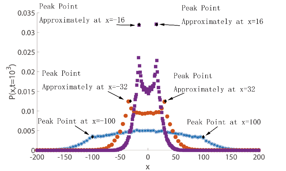
By comparing the PDFs, here we would like to make some notes on the major differences between the Lévy walk with constant velocity and with the velocity depending on the moving length ρ\rho of each step. The dotted line in Fig. 5 is for the Lévy walk with velocity v=1v=1, while the taller one is for the Lévy walk with velocity v⁡(ρ)=1/ρv(\rho)=1/\rho; their walking length density is λ⁡(ρ)=α/(1+ρ)1+α\lambda(\rho)=\alpha/(1+\rho)^{1+\alpha} with α=1.5\alpha=1.5. It can be seen that the main feature of the PDF for nonconstant v⁡(ρ)v(\rho) is the appearance of ‘U’ shape; more details, including the dependence of the shape on the parameters, will be discussed in the next paragraph. Now, we first turn to discuss the position of the high peak of the PDF. For the Lévy walk (starting from the origin) with velocity v⁡(ρ)=1/ρnv(\rho)=1/\rho^{n} and n>0n>0, or equivalently v(τ)=f−1(τ)/τ=τ−n/(n+1)\mathrm{v}(\tau)=f^{-1}(\tau)/\tau=\tau^{-n/(n+1)}, the position of the particle is ±v⁡(t)​t=±t1/(n+1)\pm\mathrm{v}(t)t=\pm t^{1/(n+1)} if the particle does not finish its first step till time tt, otherwise the farthest position that the particle can reach is bigger than t1/(n+1)t^{1/(n+1)} since t11/(n+1)+t21/(n+1)>(t1+t2)1/(n+1)t_{1}^{1/(n+1)}+t_{2}^{1/(n+1)}>(t_{1}+t_{2})^{1/(n+1)}. From the simulations shown in Fig. 6, one can note that ±t1/(n+1)\pm t^{1/(n+1)} are the positions of the high peaks of the PDF if it has.

Refer to caption
Figure 5: Comparison of the PDFs of ordinary Lévy walk and Lévy walk with the velocity v⁡(ρ)=1/ρnv(\rho)=1/\rho^{n} by sampling over 10510^{5} realizations. The flatter one is symmetric Lévy walk (at time t=103t=10^{3}) with v=1v=1 and walking length distribution λ⁡(ρ)=α/(1+ρ)1+α\lambda(\rho)=\alpha/(1+\rho)^{1+\alpha}, where α=1.5\alpha=1.5. All the parameters of the taller one with a ‘U’ shape are the same as the ones of the flatter one except v=1/ρv=1/\rho.
Refer to caption
Figure 6: (Colored online) Simulations of PDFs of symmetric Lévy walks with the velocity v=1/ρnv=1/\rho^{n} by sampling over 10510^{5} realizations at time t=103t=10^{3}. All the walking length distributions are the same, being λ⁡(ρ)=α/(1+ρ)α\lambda(\rho)=\alpha/(1+\rho)^{\alpha} with α=1.5\alpha=1.5. The velocities are chosen as v=1/ρnv=1/\rho^{n} respectively with the parameter n=0.5n=0.5 (blue stars), n=1n=1 (orange circles), and n=1.5n=1.5 (purple squares).

According to Fig. 6, it also turns out that the ‘U’ shape doesn’t always appear. More precisely, Fig. 7 shows that the shapes of PDF relate to the choice of α\alpha. For 0<α<10<\alpha<1, the ‘U’ shape always exists; for 1<α<21<\alpha<2 and n>1n>1, the ‘U’ shape can also be observed (not shown in Fig. 7); for 1<α<21<\alpha<2 and 0<n<10<n<1, the ‘U’ shape disappears, however there are still 2 sharp points at x=±t1/(n+1)x=\pm t^{1/(n+1)}, respectively; for α>2\alpha>2 and 0<n<10<n<1, the PDF turns out to be smooth. Besides from Fig. 8, it can be observed that if taking α>2\alpha>2 and n>2n>2, when tt is large enough, the ‘U’ shape gradually disappears. The above phenomena may be considered as the effect of heavy tail. When 0<α<10<\alpha<1, due to the dominant effect of heavy tail, there is a big probability that the particle hasn’t finished its first step, and it will cause peaks around the points ±v⁡(τ)​τ\pm\mathrm{v}(\tau)\tau. For the other cases, the tail becomes less heavy, so it forms a competition between α\alpha and nn.

Refer to caption
Figure 7: (Colored online) Simulations of PDFs of symmetric Lévy walks with velocity v=1/ρnv=1/\rho^{n} at time t=103t=10^{3}, by choosing different walking length distribution and sampling over 10510^{5} realizations. The walking length distributions are λ⁡(ρ)=α/(1+ρ)1+α\lambda(\rho)=\alpha/(1+\rho)^{1+\alpha} with the parameters taken as n=0.5n=0.5, t=103t=10^{3}, α=0.5\alpha=0.5 (dotted line with red squares), α=1.5\alpha=1.5 (dashed line with orange circles), and α=2.5\alpha=2.5 (real line with purple stars).
Refer to caption
Figure 8: Simulations of PDFs of symmetric Lévy walks with velocity v=1/ρ1.5v=1/\rho^{1.5} at different times by sampling over 10510^{5} realizations. The walking length distributions are the same, λ⁡(ρ)=α/(1+ρ)1+α,α=1.5\lambda(\rho)=\alpha/(1+\rho)^{1+\alpha},\alpha=1.5; while the observation times are t=104t=10^{4} and t=102t=10^{2} (the inner picture).

IV Lévy walk with velocity depending on the current position

In this section, we discuss the Lévy walk with velocity depending on the current position, i.e., v=v⁡(x)v=v(x). As a concrete example, we take v⁡(x)=v0−cτ​xv(x)=v_{0}-\frac{c}{\tau}x, where cc is a positive constant, and v0v_{0} is a non-zero constant. It seems that the integral transform method does not work for this model, and we have to resort to Hermite polynomial expansion approach. When v0=0v_{0}=0 or c=1c=1, the model will be trivial. If v0=0v_{0}=0, the particle will soon be attracted to the position x=0x=0, meaning P⁡(x,t)=δ⁡(x)P(x,t)=\delta(x) after a long time. If c=1c=1, then δ⁡(ρ+(cτ​(x−ρ)−v0)​τ)=δ⁡(x−v0​τ)\delta(\rho+(\frac{c}{\tau}(x-\rho)-v_{0})\tau)=\delta(x-v_{0}\tau). The governing equation of q⁡(x,t)q(x,t) becomes

q⁡(x,t)=∫−∞∞∫0tq⁡(x−ρ,t−τ)​ϕ​(τ)⋅δ⁡(x−v0​τ)​d​τ​d​ρ+P0​(x)​δ​(t).\begin{split}&q(x,t)\\ &=\int_{-\infty}^{\infty}\int_{0}^{t}q(x-\rho,t-\tau)\phi(\tau)\\ &~~~\cdot\delta\big(x-v_{0}\tau\big)d\tau d\rho+P_{0}(x)\delta(t).\end{split} (68)

In the following, we assume that c≠1c\neq 1 and v0≠0v_{0}\neq 0. After some calculations, there exists

q⁡(x,t)=1|c−1|​∫0tq⁡(v0​τ−xc−1,t−τ)​ϕ​(τ)​𝑑τ+P0​(x)​δ​(t).q(x,t)=\frac{1}{|c-1|}\int_{0}^{t}q\bigg(\frac{v_{0}\tau-x}{c-1},t-\tau\bigg)\phi(\tau)d\tau+P_{0}(x)\delta(t). (69)

Here we still use Hermite polynomials in (4) to approach q⁡(x,t)q(x,t). After multiplying Hm​(x)H_{m}(x) and integrating with respect to xx, we have

π​2m​m!​Tm​(t)=∑n=0∞∫0t1|c−1|​∫−∞∞Hn​(v0​τ−xc−1)​Tn​(t−τ)​Hm​(x)​𝑑x⋅ϕ⁡(τ)​d​τ+Hm​(x0)​δ​(t).\begin{split}&\sqrt{\pi}2^{m}m!T_{m}(t)\\ &=\sum_{n=0}^{\infty}\int_{0}^{t}\frac{1}{|c-1|}\int_{-\infty}^{\infty}H_{n}\bigg(\frac{v_{0}\tau-x}{c-1}\bigg)T_{n}(t-\tau)H_{m}(x)dx\\ &~~~~\cdot\phi(\tau)d\tau+H_{m}(x_{0})\delta(t).\end{split} (70)

First note that

1|c−1|​∫−∞∞Hn​(v0​τ−xc−1)​exp⁡(−(v0​τ−xτ−1)2)⋅Hm​(x)​d​x=∫−∞∞Hn​(y)​exp⁡(−y2)​Hm​(v0​τ−(c−1)​y)​dy.\begin{split}&\frac{1}{|c-1|}\int_{-\infty}^{\infty}H_{n}\left(\frac{v_{0}\tau-x}{c-1}\right)\exp\left(-\left(\frac{v_{0}\tau-x}{\tau-1}\right)^{2}\right)\\ &~~~~\cdot H_{m}(x)dx\\ &=\int_{-\infty}^{\infty}H_{n}(y)\exp(-y^{2})H_{m}(v_{0}\tau-(c-1)y)dy.\end{split} (71)

Then basing on the properties of Hermite polynomials (96), (98), and (99), the equation for Hm​(v0​τ−(c−1)​y)H_{m}(v_{0}\tau-(c-1)y) can be obtained as

Hm​(v0​τ−(c−1)​y)=∑k=0mm!k!​(m−k)!​Hk​(−(c−1)​y)​(2​v0​τ)m−k=∑k=0mm!(m−k)!​(2​v0​τ)m−k​∑i=0⌊k2⌋(1−c)k−2​i​(c2−2​c)i(k−2​i)!​i!⋅Hk−2​i​(x).\begin{split}&H_{m}(v_{0}\tau-(c-1)y)\\ &=\sum_{k=0}^{m}\frac{m!}{k!(m-k)!}H_{k}(-(c-1)y)(2v_{0}\tau)^{m-k}\\ &=\sum_{k=0}^{m}\frac{m!}{(m-k)!}(2v_{0}\tau)^{m-k}\sum_{i=0}^{\lfloor\frac{k}{2}\rfloor}\frac{(1-c)^{k-2i}(c^{2}-2c)^{i}}{(k-2i)!i!}\\ &~~~~\cdot H_{k-2i}(x).\end{split} (72)

Substituting (72) into (70) and taking Laplace transform w.r.t. tt lead to the recurrence relation

π​2m​m!​T^m​(s)=∑k=0m∑i=0⌊k2⌋m!​2m−2​i​π(m−k)!​i!​T^k−2​i​(s)⋅ℒτ→s​{(v0​τ)m−k​(1−c)k−2​i​(c2−2​c)i​ϕ​(τ)}+Hm​(x0).\begin{split}&\sqrt{\pi}2^{m}m!\hat{T}_{m}(s)\\ &=\sum_{k=0}^{m}\sum_{i=0}^{\lfloor\frac{k}{2}\rfloor}\frac{m!2^{m-2i\sqrt{\pi}}}{(m-k)!i!}\hat{T}_{k-2i}(s)\\ &~~~~\cdot\mathcal{L}_{\tau\rightarrow s}\{(v_{0}\tau)^{m-k}(1-c)^{k-2i}(c^{2}-2c)^{i}\phi(\tau)\}\\ &~~~~+H_{m}(x_{0}).\end{split} (73)

From (73), we can obtain

T^0​(s)\displaystyle\hat{T}_{0}(s) =\displaystyle= 1π​(1−ϕ^​(s)),\displaystyle\frac{1}{\sqrt{\pi}(1-\hat{\phi}(s))}, (74)
T^1​(s)\displaystyle\hat{T}_{1}(s) =\displaystyle= −x0+x0​ϕ^​(s)+v0​ϕ^′​(s)π​(ϕ^​(s)−1)​(1+(c−1)​ϕ^​(s)),\displaystyle\frac{-x_{0}+x_{0}\hat{\phi}(s)+v_{0}\hat{\phi}^{\prime}(s)}{\sqrt{\pi}(\hat{\phi}(s)-1)(1+(c-1)\hat{\phi}(s))}, (75)

and

π​23​T^2​(s)=22​π​v02​ϕ^′′​(s)​T^0​(s)−23​π​v0​(1−c)⋅ϕ^′​(s)​T^1​(s)+23​π​(1−c)2​ϕ^​(s)​T^2​(s)+2​π​(c2−2​c)​ϕ^​(s)​T^0​(s)+H2​(x0).\begin{split}\sqrt{\pi}2^{3}\hat{T}_{2}(s)=&2^{2}\sqrt{\pi}v_{0}^{2}\hat{\phi}^{\prime\prime}(s)\hat{T}_{0}(s)-2^{3}\sqrt{\pi}v_{0}(1-c)\\ &\cdot\hat{\phi}^{\prime}(s)\hat{T}_{1}(s)+2^{3}\sqrt{\pi}(1-c)^{2}\hat{\phi}(s)\hat{T}_{2}(s)\\ &+2\sqrt{\pi}(c^{2}-2c)\hat{\phi}(s)\hat{T}_{0}(s)+H_{2}(x_{0}).\end{split} (76)

Then we consider the PDF of finding the particle at position xx at time tt, which can be obtained as

P⁡(x,t)=∫−∞∞d​y​∫0tq⁡(x−y,t−τ)​Ψ​(τ)⋅δ⁡(y+(cτ​(x−y)−v0)​τ)​d​τ.\begin{split}P(x,t)=&\int_{-\infty}^{\infty}dy\int_{0}^{t}q(x-y,t-\tau)\Psi(\tau)\\ &\cdot\delta\Big(y+\Big(\frac{c}{\tau}(x-y)-v_{0}\Big)\tau\Big)d\tau.\end{split} (77)

Rewrite P⁡(x,t)P(x,t) as the form of (5). After taking Laplace transform w.r.t. tt, we have

T~^m​(s)=∑k=0m∑i=0⌊k2⌋2−2​i(m−k)!​i!​T^k−2​i​(s)⋅ℒτ→s​{(v0​τ)m−k​(1−c)k−2​i​(c2−2​c)i​Ψ​(τ)}.\begin{split}&\hat{\tilde{T}}_{m}(s)\\ &=\sum_{k=0}^{m}\sum_{i=0}^{\lfloor\frac{k}{2}\rfloor}\frac{2^{-2i}}{(m-k)!i!}\hat{T}_{k-2i}(s)\\ &~~~\cdot\mathcal{L}_{\tau\rightarrow s}\{(v_{0}\tau)^{m-k}(1-c)^{k-2i}(c^{2}-2c)^{i}\Psi(\tau)\}.\end{split} (78)

Then

T~^0​(s)=Ψ^​(s)​T^0​(s)=1π​s,T~^1​(s)=−v0​Ψ^′​(s)​T^0​(s)+(1−c)​Ψ^​(s)​T^1​(s),T~^2​(s)=12​v02​Ψ^′′​(s)​T^0​(s)−v0​(1−c)​Ψ^′​(s)​T^1​(s)+(1−c)2​Ψ^​(s)​T^2​(s)+14​(c2−2​c)​Ψ^​(s)​T^0​(s).\begin{split}\hat{\tilde{T}}_{0}(s)&=\hat{\Psi}(s)\hat{T}_{0}(s)=\frac{1}{\sqrt{\pi}s},\\ \hat{\tilde{T}}_{1}(s)&=-v_{0}\hat{\Psi}^{\prime}(s)\hat{T}_{0}(s)+(1-c)\hat{\Psi}(s)\hat{T}_{1}(s),\\ \hat{\tilde{T}}_{2}(s)&=\frac{1}{2}v_{0}^{2}\hat{\Psi}^{\prime\prime}(s)\hat{T}_{0}(s)-v_{0}(1-c)\hat{\Psi}^{\prime}(s)\hat{T}_{1}(s)\\ &~~~~+(1-c)^{2}\hat{\Psi}(s)\hat{T}_{2}(s)+\frac{1}{4}(c^{2}-2c)\hat{\Psi}(s)\hat{T}_{0}(s).\end{split} (79)

According to (5), there exists

⟨x⁡(s)⟩=π​T~^1​(s)⟨x2​(s)⟩=π2​T~^0​(s)+2​π​T~^2​(s)=12​s+2​π​T~^2​(s).\begin{split}\big<x(s)\big>&=\sqrt{\pi}\hat{\tilde{T}}_{1}(s)\\ \big<x^{2}(s)\big>&=\frac{\sqrt{\pi}}{2}\hat{\tilde{T}}_{0}(s)+2\sqrt{\pi}\hat{\tilde{T}}_{2}(s)\\ &=\frac{1}{2s}+2\sqrt{\pi}\hat{\tilde{T}}_{2}(s).\end{split} (80)

In the following, we consider different kinds of flight time distributions ϕ⁡(τ)\phi(\tau). First we investigate the power-law flight time as the form shown in (23). For 0<α<10<\alpha<1, ϕ^​(s)∼1−Γ⁡(1−α)​sα\hat{\phi}(s)\sim 1-\Gamma(1-\alpha)s^{\alpha}. After some calculations, we can obtain

⟨x⁡(s)⟩\displaystyle\big<x(s)\big> ∼\displaystyle\sim (1−α)​v0s2,\displaystyle\frac{(1-\alpha)v_{0}}{s^{2}}, (81)
⟨x2​(s)⟩\displaystyle\big<x^{2}(s)\big> ∼\displaystyle\sim (2−α)​(1−α)​v02s3.\displaystyle\frac{(2-\alpha)(1-\alpha)v_{0}^{2}}{s^{3}}. (82)

Thus the corresponding inverse Laplace transforms are

⟨x⁡(t)⟩\displaystyle\big<x(t)\big> ∼\displaystyle\sim (1−α)​v0​t,\displaystyle(1-\alpha)v_{0}t, (83)
⟨x2​(t)⟩\displaystyle\big<x^{2}(t)\big> ∼\displaystyle\sim (2−α)​(1−α)​v022​t2.\displaystyle\frac{(2-\alpha)(1-\alpha)v_{0}^{2}}{2}t^{2}. (84)

For 1<α<21<\alpha<2, ϕ^​(s)∼1−1α−1​s−Γ⁡(1−α)​sα\hat{\phi}(s)\sim 1-\frac{1}{\alpha-1}s-\Gamma(1-\alpha)s^{\alpha}, and

⟨x⁡(t)⟩\displaystyle\big<x(t)\big> =\displaystyle= (α−1)​v02−α​t2−α,\displaystyle\frac{(\alpha-1)v_{0}}{2-\alpha}t^{2-\alpha}, (85)
⟨x2​(t)⟩\displaystyle\big<x^{2}(t)\big> =\displaystyle= (α−1)​v023−α​t3−α.\displaystyle\frac{(\alpha-1)v_{0}^{2}}{3-\alpha}t^{3-\alpha}. (86)

For the exponential distribution, we simply consider the Laplace transform with the form of ϕ^​(s)=11+s\hat{\phi}(s)=\frac{1}{1+s}. Then

⟨x⁡(t)⟩\displaystyle\big<x(t)\big> =\displaystyle= v0c,\displaystyle\frac{v_{0}}{c}, (87)
⟨x2​(t)⟩\displaystyle\big<x^{2}(t)\big> =\displaystyle= 2​v02(2−c)​c2for​c<2,\displaystyle\frac{2v_{0}^{2}}{(2-c)c^{2}}~~~~\mathrm{for}~~c<2, (88)
⟨x2​(t)⟩\displaystyle\big<x^{2}(t)\big> =\displaystyle= v02​tfor​c=2,\displaystyle v_{0}^{2}t~~~~~~~~~~~~\mathrm{for}~~c=2, (89)

According to (87) and (88), it turns out that the particle has a localization. The results above are verified by the numerical simulations shown in Fig. 9.

Refer to caption
Refer to caption
Figure 9: Simulations of MSD of Lévy walk with velocity v⁡(x)=v0−cτ​xv(x)=v_{0}-\frac{c}{\tau}x. Each dot is obtained by averaging over 10410^{4} realizations. The above figure shows the simulations of MSD of Lévy walk with α=0.5\alpha=0.5, c=1.5c=1.5 (circles) and α=1.5\alpha=1.5, c=1.5c=1.5 (squares). The lower one illustrates the Lévy walk with ϕ⁡(τ)=exp⁡(−τ)\phi(\tau)=\exp(-\tau), and c=2c=2 (circles), c=1.5c=1.5 (squares in the inner figure).

V Conclusion

This paper discusses the Lévy walk with velocity depending on walking length or walking time of each step, and with velocity being a function of current position. When doing the dynamical analyses of the Lévy walk, we introduce the Hermite polynomial expansion approach, which can be effectively used to analyze the time-space coupled or nonlinear models. This approach is an important complement to integral transform method. Both the integral transform method and Hermite polynomial expansion approach work for the Lévy walk with velocity depending on walking length or walking time of each step. One of the striking results is that when v⁡(ρ)=1/ρv(\rho)=1/\rho the process will always show a normal diffusion, no matter what kind of walking length distribution is. By numerical simulations, the rich structure information of the PDF is uncovered. As for the Lévy walk with velocity being a function of current position, we use the Hermite polynomial expansion approach to do the analysis with also some interesting phenomena uncovered. This kind of orthogonal polynomial approaches will be further developed in the coming researches.

Acknowledgements

This work was supported by the National Natural Science Foundation of China under grant no. 11671182, and the Fundamental Research Funds for the Central Universities under grant no. lzujbky-2018-ot03.

Appendix A A brief introduction of Meijer G-function and generalized hypergeometric function

Here we only briefly introduce the definition and some important properties of Meijer G-function. For more details, one can refer to A. P. Prudnikov and Marichev 1990. The Meijier G-function of order (m,n,p,q)(m,n,p,q), where 0≤m≤q0\leq m\leq q and 0≤n≤p0\leq n\leq p, is defined as

Gp,qm,n​(z|(ap)(bq))≡Gp,qm,n​(z|a1,…,apb1,…,bq)=12​π​i​∫LΓ⁡[b1+s,…,bm+s,1−a1−s,…,1−an−san+1+s,…,ap+s,1−bm+1−s,…,1−bq−s]​z−s​𝑑s;G_{p,q}^{m,n}\bigg(z\bigg|\begin{matrix}(a_{p})\\ (b_{q})\end{matrix}\bigg)\equiv G_{p,q}^{m,n}\bigg(z\bigg|\begin{matrix}a_{1},\ldots,a_{p}\\ b_{1},\ldots,b_{q}\end{matrix}\bigg)=\frac{1}{2\pi i}\int_{L}\Gamma\bigg[\begin{matrix}b_{1}+s,\ldots,b_{m}+s,1-a_{1}-s,\ldots,1-a_{n}-s\\ a_{n+1}+s,\ldots,a_{p}+s,1-b_{m+1}-s,\ldots,1-b_{q}-s\end{matrix}\bigg]z^{-s}ds; (90)

where LL is a contour defined in A. P. Prudnikov and Marichev 1990. One of the most important properties of Meijer G-function is the representation of generalized hypergeometric functions

Gp,qm,n​(z|(ap)(bq))==∑k=1nΓ⁡[ak−a1,…,ak−ak−1,ak−ak+1,…,ak−an,1+b1−ak,…,1+bm−akak−bm+1,…,ak−bq,1+an+1−ak,…,1+ap−ak]​zak−1⋅Fp−1q​(1+(bq)−ak1+(ap)∗−ak,(−1)q−m−nz)\begin{split}&G_{p,q}^{m,n}\bigg(z\bigg|\begin{matrix}(a_{p})\\ (b_{q})\end{matrix}\bigg)=\\ &=\sum_{k=1}^{n}\Gamma\bigg[\begin{matrix}a_{k}-a_{1},\ldots,a_{k}-a_{k-1},a_{k}-a_{k+1},\ldots,a_{k}-a_{n},1+b_{1}-a_{k},\ldots,1+b_{m}-a_{k}\\ a_{k}-b_{m+1},\ldots,a_{k}-b_{q},1+a_{n+1}-a_{k},\ldots,1+a_{p}-a_{k}\end{matrix}\bigg]z^{a_{k}-1}\\ &~~~\cdot{{}_{q}F_{p-1}}\bigg(\begin{matrix}1+(b_{q})-a_{k}\\ 1+(a_{p})^{*}-a_{k}\end{matrix};\frac{(-1)^{q-m-n}}{z}\bigg)\end{split} (91)

under the assumptions p≥qp\geq q; aj−ak≠0,±1,±2,⋯a_{j}-a_{k}\neq 0,\pm 1,\pm 2,\cdots; j≠kj\neq k; j,k=1,2,⋯,nj,k=1,2,\cdots,n, and some requests on the contour LL. Here (ap)∗−ak≡a1−ak,⋯,ak−1−ak,ak+1−ak,⋯,ap−ak(a_{p})^{*}-a_{k}\equiv a_{1}-a_{k},\cdots,a_{k-1}-a_{k},a_{k+1}-a_{k},\cdots,a_{p}-a_{k};

Γ⁡[a1,⋯,apb1,⋯,bq]=∏k=1pΓ⁡(ak)∏l=1qΓ⁡(bl),\Gamma\bigg[\begin{matrix}a_{1},\cdots,a_{p}\\ b_{1},\cdots,b_{q}\end{matrix}\bigg]=\frac{\prod_{k=1}^{p}\Gamma(a_{k})}{\prod_{l=1}^{q}\Gamma(b_{l})}, (92)

and the function Fp−1q{}_{q}F_{p-1} in (91) represents the generalized hypergeometric function, which is defined as

pFq(a1,⋯,apb1,⋯,bq;z)=∑n=0∞(a1)n⋯(ap)n(b1)n⋯(bq)nznn!_{p}F_{q}\bigg(\begin{matrix}a_{1},\cdots,a_{p}\\ b_{1},\cdots,b_{q}\end{matrix};z\bigg)=\sum_{n=0}^{\infty}\frac{(a_{1})_{n}\cdots(a_{p})_{n}}{(b_{1})_{n}\cdots(b_{q})_{n}}\frac{z^{n}}{n!} (93)

with (a)0=1(a)_{0}=1 and (a)n=a(a+1)(a+2)⋯(a+n−1)(a)_{n}=a(a+1)(a+2)\cdots(a+n-1) for n≥1n\geq 1.

Appendix B A brief introduction to Hermite polynomials and orthogonal polynomials

For a system of polynomials fn​(x)f_{n}(x) with degree [fn​(x)]=n[f_{n}(x)]=n, if there is a function ω(x)[ω(x)≥0]\omega(x)\,[\omega(x)\geq 0] on the interval a≤x≤ba\leq x\leq b such that

∫abfn​(x)​fm​(x)​ω​(x)​𝑑x=0,\int_{a}^{b}f_{n}(x)f_{m}(x)\omega(x)dx=0, (94)

for n≠mn\neq m with n,m=0,1,2,⋯n,m=0,1,2,\cdots, then the system of polynomials fn​(x)f_{n}(x) is called orthogonal on the interval a≤x≤ba\leq x\leq b w.r.t. the weight function ω⁡(x)\omega(x) Abramowitz and Stegun 1972. Following different kinds of weight functions and/or intervals, there are the corresponding orthogonal polynomials A. P. Prudnikov and Marichev 1990; Abramowitz and Stegun 1972. One of the most important kind of orthogonal polynomials defined on (−∞,∞)(-\infty,\infty) are Hermite polynomials with the weight function ω⁡(x)=e−x2\omega(x)=e^{-x^{2}}. It can also be calculated as

Hn​(x)=(−1)n​ex2​dnd​xn​e−x2.H_{n}(x)=(-1)^{n}e^{x^{2}}\frac{d^{n}}{dx^{n}}e^{-x^{2}}. (95)

Its orthogonality is given as

∫−∞∞Hm​(x)​Hn​(x)​e−x2​𝑑x=π​2n​n!​δn,m,\int_{-\infty}^{\infty}H_{m}(x)H_{n}(x)e^{-x^{2}}dx=\sqrt{\pi}2^{n}n!\delta_{n,m}, (96)

where δn,m\delta_{n,m} is the Kronecker delta function. Here we only illustrate some of the important properties of Hermite polynomials. The values of Hermite polynomials at 00 are very useful

Hn​(0)={0if n is odd,(−2)n2​(n−1)!!if n is even,H_{n}(0)=\begin{cases}0&\mbox{if $n$ is odd},\\ (-2)^{\frac{n}{2}}(n-1)!!&\mbox{if $n$ is even},\end{cases} (97)

which indicates the recursion relation Hn​(0)=−2​(n−1)​Hn−2​(0)H_{n}(0)=-2(n-1)H_{n-2}(0). Besides the following two expressions are also important in this paper:

Hn​(x+y)=∑k=0n(nk)​Hk​(x)​(2​y)n−kH_{n}(x+y)=\sum_{k=0}^{n}\bigg(\begin{matrix}n\\ k\end{matrix}\bigg)H_{k}(x)(2y)^{n-k} (98)

and

Hn​(γ​x)=∑i=0⌊n2⌋γn−2​i​(γ2−1)i​(n2​i)​(2​i)!i!​Hn−2​i​(x),H_{n}(\gamma x)=\sum_{i=0}^{\lfloor\frac{n}{2}\rfloor}\gamma^{n-2i}(\gamma^{2}-1)^{i}\bigg(\begin{matrix}n\\ 2i\end{matrix}\bigg)\frac{(2i)!}{i!}H_{n-2i}(x), (99)

where ⌊n2⌋\lfloor\frac{n}{2}\rfloor is the biggest integer smaller than n2\frac{n}{2}.

References

  • Golding and Cox (2006) I. Golding and E. C. Cox, Physical nature of bacterial cytoplasm, Phys. Rev. Lett. 96, 098102 (2006).
  • Metzler and Klafter (2000) R. Metzler and J. Klafter, The random walk’s guide to anomalous diffusion: a fractional dynamics approach, Phys. Rep. 339, 1 (2000).
  • Weiss (1994) G. H. Weiss, Aspects and Applications of the Random Walk (North-Holland Publishing Co., Amsterdam, 1994).
  • Coffey et al. (2004) W. T. Coffey, Y. P. Kalmykov, and J. T. Waldron, The Langevin Equation (World Scientific Publishing Co. Pte. Ltd., Singapore, 2004).
  • Deng and Zhang (2019) W. H. Deng and Z. J. Zhang, High Accuracy Algorithm for the Differential Equations Governing Anomalous Diffusion (World Scientific Publishing Co. Pte. Ltd., Singapore, 2019).
  • Cartea and del Castillo-Negrete (2007) A. Cartea and D. del Castillo-Negrete, Fluid limit of the continuous-time random walk with general Lévy jump distribution functions, Phys. Rev. E 76, 041105 (2007).
  • Metzler et al. (2014) R. Metzler, J.-H. Jeon, A. G. Cherstvy, and E. Barkai, Anomalous diffusion models and their properties: non-stationarity, non-ergodicity, and ageing at the centenary of single particle tracking, Phys. Chem. Chem. Phys. 16, 24128 (2014).
  • Fogedby (1994) H. C. Fogedby, Langevin equations for continuous time Lévy flights, Phys. Rev. E 50, 1657 (1994).
  • Magdziarz et al. (2007) M. Magdziarz, A. Weron, and K. Weron, Fractional Fokker-Planck dynamics: Stochastic representation and computer simulation, Phys. Rev. E 75, 016708 (2007).
  • Zaburdaev et al. (2015) V. Zaburdaev, S. Denisov, and J. Klafter, Lévy walks, Rev. Mod. Phys. 87, 483 (2015).
  • Zaburdaev et al. (2016) V. Zaburdaev, I. Fouxon, S. Denisov, and E. Barkai, Superdiffusive dispersals impart the geometry of underlying random walks, Phys. Rev. Lett. 117, 270601 (2016).
  • Zaburdaev et al. (2008) V. Zaburdaev, M. Schmiedeberg, and H. Stark, Random walks with random velocities, Phys. Rev. E 78, 011119 (2008).
  • Xu and Deng (2018) P. B. Xu and W. H. Deng, Lévy walk with multiple internal states, J. Stat. Phys. 173, 1598 (2018).
  • Dentz et al. (2015) M. Dentz, T. Le Borgne, D. R. Lester, and F. P. J. de Barros, Scaling forms of particle densities for Lévy walks and strong anomalous diffusion, Phys. Rev. E 92, 032128 (2015).
  • Gajda and Magdziarz (2010) J. Gajda and M. Magdziarz, Fractional Fokker-Planck equation with tempered α\alpha-stable waiting times: Langevin picture and computer simulation, Phys. Rev. E 82, 011117 (2010).
  • Sandev et al. (2018) T. Sandev, W. H. Deng, and P. B. Xu, Models for characterizing the transition among anomalous diffusions with different diffusion exponents, J. Phys. A: Math. Theor. 51, 405002 (2018).
  • Krüsemann et al. (2014) H. Krüsemann, A. c. v. Godec, and R. Metzler, First-passage statistics for aging diffusion in systems with annealed and quenched disorder, Phys. Rev. E 89, 040101 (2014).
  • Deng et al. (2017) W. H. Deng, X. C. Wu, and W. L. Wang, Mean exit time and escape probability for the anomalous processes with the tempered power-law waiting times, EPL 117, 10009 (2017).
  • Dybiec and Sokolov (2015) B. Dybiec and I. M. Sokolov, Estimation of the smallest eigenvalue in fractional escape problems: Semi-analytics and fits, Comput. Phys. Comm. 187, 29 (2015).
  • A. P. Prudnikov and Marichev (1990) Y. A. B. A. P. Prudnikov and O. I. Marichev, Integral and Series (Gordon and Breach Science Publishers, New York, 1990).
  • Abramowitz and Stegun (1972) M. Abramowitz and I. A. Stegun, Handbook of Mathematical Functions with Formulas, Graphs, and Mathematical Tables (United States Department of Commerce, Washington D.C., 1972).