Giant Orbital Magnetoelectric effect and Current-induced Magnetization Switching in Twisted Bilayer Graphene

An isolated TBG can be described by coupling the top and bottom graphene layers with a twist angle $\theta$. Near the Fermi energy, the top and bottom graphene layers with the Dirac Hamiltonian at the valley $\xi$ can be described by a continuum model as Neto1; Neto2; MacDonald:

where $\mathcal{H}_{\textrm{t}/\textrm{b}}$ denotes the Hamiltonian of the top and bottom layer respectively, $a^{\left(\dagger\right)}_{\textrm{t}/\textrm{b},s,\xi}\left({\bf q}\right)$ is a two component creation (annihilation) operator creating (annihilating) electrons at the two A and B sublattices in the top/bottom graphene layer. The valley and the spin indices are denoted by $\xi=\pm 1$ and $s=\uparrow,\downarrow$ respectively. The momentum ${\bf q}={\bf k}-{\bf K}_{\xi}$ is defined relative to the original Brillouin zone corner that hosts the Dirac point at ${\bf K}_{\xi}$, $d=1.42\AA$ is the carbon-carbon bond length Neto5, the rotation matrix has the form ${\bf\hat{R}}_{\pm\frac{\theta}{2}}=\cos\frac{\theta}{2}\mp i\sigma_{y}\sin\frac{\theta}{2}$, the Fermi velocity takes the value $\hbar v_{\textrm{F}}=5.96$eV$\AA$ Neto5 and ${\bf\sigma}=\left(\sigma_{x},\sigma_{y}\right)$ denotes the Pauli matrices.

An important effect of the moiré superlattice which originates from twisting is to fold the original Brillouin zone into the mini-Brillouin zones schematically shown in Fig. 1a. Both the ${\bf K}_{+}$ and ${\bf K}_{-}$ points of the original Brillouin zone are mapped to the mini-Brillouin zone, giving rise to four-fold degenerate minbands with both valley and spin degeneracy. In the reciprocal space, the Moiré superlattice has reciprocal vectors ${\bf q}_{\textrm{b}}=\frac{8\pi\sin\frac{\theta}{2}}{3\sqrt{3}d}\left(0,-1\right)$, ${\bf q}_{\textrm{tr}}=\frac{8\pi\sin\frac{\theta}{2}}{3\sqrt{3}d}\left(\frac{\sqrt{3}}{2},\frac{1}{2}\right)$, ${\bf q}_{\textrm{tl}}=\frac{8\pi\sin\frac{\theta}{2}}{3\sqrt{3}d}\left(-\frac{\sqrt{3}}{2},\frac{1}{2}\right)$ connecting the three neighboring sites of the hexagonal receiprocal lattice. The interlayer coupling is enabled when the momentum transfer between the Bloch states at different layers matches ${\bf q}_{\textrm{b}}$, ${\bf q}_{\textrm{tr}}$ or ${\bf q}_{\textrm{tl}}$. The interlayer coupling Hamiltonian of the continuum model Neto1; Neto2; MacDonald is present in the Methods Section.

For an isolated TBG, the top and bottom graphene Hamiltonian along with the interlayer coupling respects the D₆ symmetry Hoi1; Liujun; Vishwanath; Balents; Bernevig. At the mini-Brillouin zone corner ${\bf K}^{m}_{\pm}$, two massless Dirac points emerge which are protected by the composite symmetry C${}_{2}\mathcal{T}$ where $\mathcal{T}$ is the complex conjugate operator Hoi1; Liujun; Balents; Bernevig. However, in the two recent experiments in which a ferromagnetic state has been seen, the TBG is coupled with a hBN cladding layer aligned to the TBG to less than 1 degree, which empirically appears necessary to support the ferromagnetism David; Young. In our model, the hBN substrate affects the bottom graphene layer in two aspects: 1) it breaks the C₂ symmetry and introduces the massive gap $\Delta\sigma_{z}$ to the Dirac Hamiltonian as shown in Fig. 1b; 2) it exerts strain on the bottom graphene layer and further reduces the crystal symmetry to C₁.

In this work, for simplicity we use a uniaxial strain tensor $\bm{\mathcal{E}}$ to describe the effect of strain. The strain tensor can be written as:

with $\varepsilon$ being the tunable parameter to characterize the strain induced displacement, $\nu=0.165$ the Poisson ratio for graphene Neto4, and $\phi$ the angle of the uniaxial strain relative to the zigzag direction of the bottom graphene layer. In the presence of uniaxial strain, the real space and reciprocal space are transformed as $\tilde{{\bf r}}=\left(1+\bm{\mathcal{E}}\right){\bf r}$ and $\tilde{{\bf k}}=\left(1-\bm{\mathcal{E}}^{\textrm{T}}\right){\bf k}$ respectively. Therefore the Dirac points in the bottom graphene layer are shifted from the original position ${\bf K}_{\xi}$ to $\left(1-\bm{\mathcal{E}^{\textrm{T}}}\right){\bf K}_{\xi}-\xi{\bf A}$, where ${\bf A}=\frac{\beta}{d}\left(\mathcal{E}_{xx}-\mathcal{E}_{yy},-2\mathcal{E}_{xy}\right)$ with $\beta=1.57$ being the effective gauge field from the strain Guinea. By combining the sublattice symmetry breaking and uniaxial strain effect from the hBN substrate, we are able to obtain the modified bottom graphene layer Hamiltonian as

where the momentum ${\bf q}={\bf k}-\left(1-\bm{\mathcal{E}}^{\textrm{T}}\right){\bf K}_{\xi}$ is defined relative to the uniaxial strain-deformed Brillouin zone corner, and the staggered potential introduced by the hBN substrate takes $\Delta=17$meV MenyoungLee; Jung. The staggered potential breaks the $C_{2z}$ symmetry and reduces $D_{6}$ to $D_{3}$ symmetry, while the uniaxial strain further removes all the crystal lattice symmetry and brings the TBG down to the $C_{1}$ group.

Denoting the interlayer coupling between the strained bottom layer graphene and the unstrained top layer graphene as $\tilde{\mathcal{H}}_{\textrm{int}}$, the total Hamiltonian can be written as

where $A_{s,\xi}\left({\bf q}\right)$ is a multicomponent operator and $h_{\xi}\left({\bf q}\right)$ is the Hamiltonian matrix as described in detail in the Methods Section.

The energy dispersion at each band for the TBG can then be directly obtained through diagonalizing the continuum Hamiltonian in Equation (4). For an isolated TBG, at the angle $\theta=1.20\degree$, the Hamiltonian with $\bm{\mathcal{E}}=0,\Delta=0$ gives the flat bands dispersion as shown in the dashed lines of Fig. 1b. The flat bands possess two gapless Dirac points at ${\bf K}^{m}_{\pm}$ in the mini-Brillouin zone. The energy dispersion with strain is depicted by the solid lines in Fig. 1b. The energy dispersion for the conduction band (the red band in Fig. 1b) in the whole Brillouin zone are shown in Fig. 1c and Fig. 1d for the unstrained and the strained cases respectively. It is clear from Fig. 1c that the energy dispersion $E_{s,\xi,\nu}\left({\bf k}\right)$ with spin index $s$, valley index $\xi$ and band index $\nu$ in general respects the C₃ symmetry as $E_{s,\xi,\nu}\left({\bf q}\right)=E_{s,\xi,\nu}\left({\bf\hat{R}}_{\frac{2\pi}{3}}{\bf q}\right)$. However, strain breaks the three-fold rotational symmetry as shown in Fig. 1d, in which we set $\varepsilon=0.1\%$ and the strain is applied along the direction of the zigzag edge of the bottom layer graphene ($\phi=0$ in Equation (2)).

With the Hamiltonian in Equation (4), we can calculate the Berry curvature $\Omega^{z}_{s,\xi,\nu}\left({\bf q}\right)$ and the orbital magnetic moment in the out-of-plane direction $m^{z}_{s,\xi,\nu}\left({\bf q}\right)$ of each Bloch state:

and

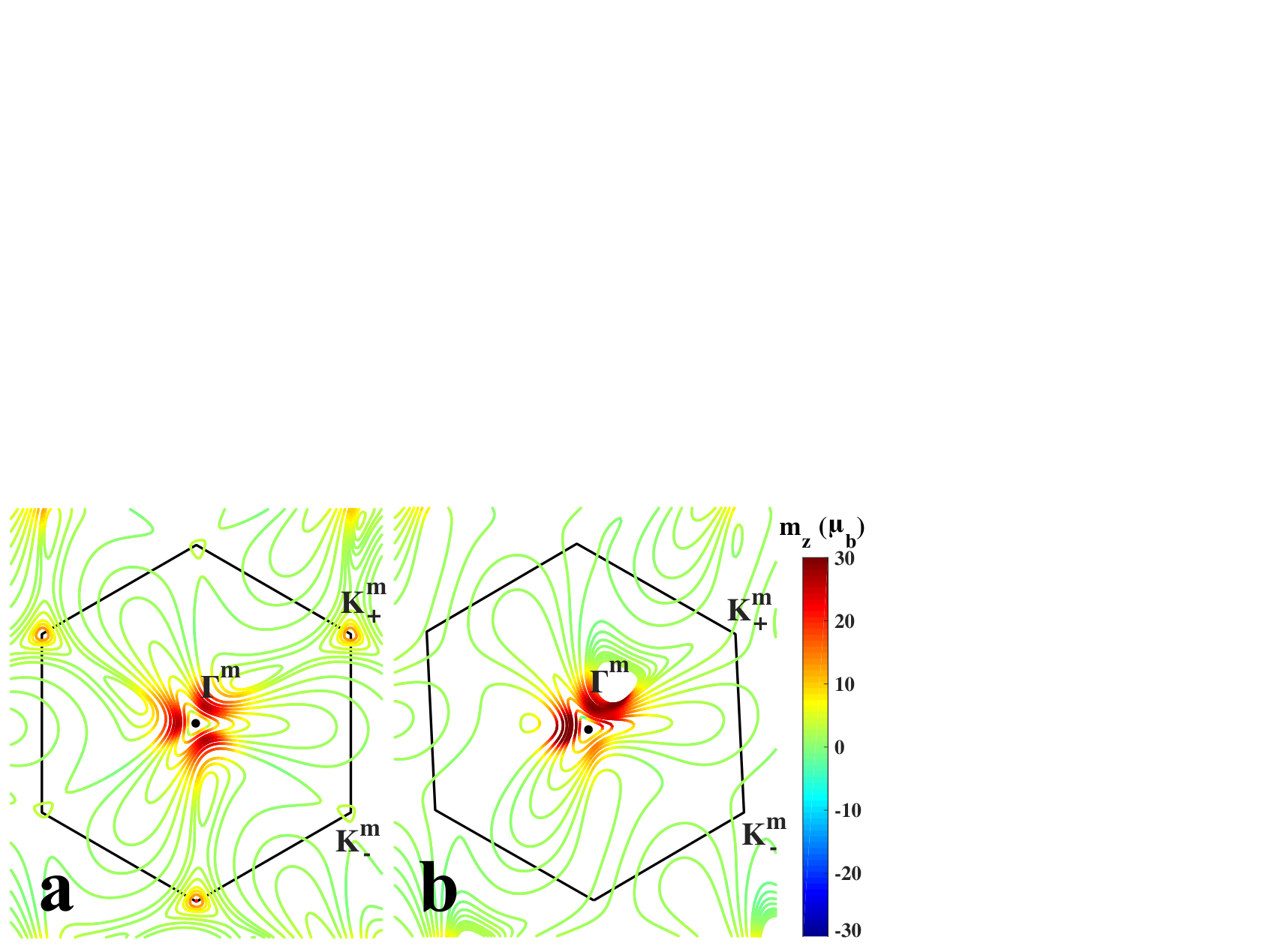
For an isolated TBG, the Berry curvature and the magnetic moment are non-zero only at the Dirac point. In the absence of strain but in the presence of the staggered potential which is set to be $\Delta=17$meV, the distribution of the orbital magnetic moment in the mini-Brillouin zone is shown in Fig. 2a. It respects the C₃ symmetry as $m^{z}_{s,\xi,\nu}\left({\bf q}\right)=m^{z}_{s,\xi,\nu}\left({\bf\hat{R}}_{\frac{2\pi}{3}}{\bf q}\right)$. The orbital magnetic moments are particularly large around ${\bf K}^{\textrm{m}}_{\xi}$ and ${\bf\Gamma}^{\textrm{m}}$ in the mini-Brillouin zone, where the flat band hybridizes with adjacent bands. The strength of the orbital magnetic moments can reach about $30\mu_{\textrm{b}}$ with $\mu_{\textrm{b}}=\frac{e\hbar}{2m_{\textrm{e}}}$ the Bohr magneton. In the presence of strain, the C_3z symmetry of $m^{z}$ is broken as shown in Fig. 2b. If time-reversal symmetry is preserved, the orbital magnetic moment has the constraint $m^{z}_{s,+,\nu}\left({\bf q}\right)=-m^{z}_{s,-,\nu}\left(-{\bf q}\right)$, so that no net magnetization is allowed. However, due to the C₃ symmetry breaking, applying a current would create an imbalance in the magnetic moment distribution and thus a net out-of-plane magnetization Wenyu1 as demonstrated in the next section.

In quasi-two-dimensional materials with finite magnetoelectric response, the electric field induced magnetization can be described as:

with $i,j=x,y$, and $\alpha_{ij}$ the magnetoelectric susceptibility. As shown in Ref. Wenyu1; Wenyu2, the general forms of the components of the magnetoelectric susceptibility tensor $\alpha_{ij}$ can be determined by the crystal symmetry of the material. The general forms of $\alpha_{ij}$ for point groups D₆, C₃ and C₁ which are relevant to TBG are shown in Table 1. It is clear from Table 1 that it is possible to generate an out-of-plane magnetization by in-plane electric fields only if the crystal point group symmetry is reduced to C₁.

To calculate $\alpha_{ij}$ for TBG, we can use the linear response theory which gives Joel; JingMa:

where $\int_{{\bf q}}\equiv\frac{1}{\left(2\pi\right)^{2}}\int_{\textrm{BZ}}d{\bf q}$, $f\left(E\right)$ is the Fermi Dirac distribution function, $v^{j}_{s,\xi,\nu}=\partial_{q_{j}}E_{s,\xi,\nu}\left({\bf q}\right)$ is the group velocity, $\tau$ is the effective scattering time, and the total magnetic moment ${\bf M}_{s,\xi,\nu}\left({\bf q}\right)={\bf m}_{s,\xi,\nu}\left({\bf q}\right)+{\bf S}_{s,\xi,\nu}\left({\bf q}\right)$ is composed of both the orbital magnetic moment ${\bf m}_{s,\xi,\nu}\left({\bf q}\right)$ and the spin magnetic moment ${\bf S}_{s,\xi,\nu}=\bra{u_{s,\xi,\nu}\left({\bf q}\right)}\frac{1}{2}g\mu_{\textrm{b}}\bm{\sigma}\ket{u_{s,\xi,\nu}\left({\bf q}\right)}$ with the Lande g factor $g=2$.

To be specific, we apply a uniaxial strain with $\varepsilon=0.1\%$ along the zig-zag edge direction of the bottom layer graphene. The orbital magnetization in the Brillouin zone in the presence of strain is shown in Fig. 2b. The resultant magnetoelectric susceptibility can then be evaluated assuming the electron scattering time to be $\tau=10$ps Polini. For the conduction band $\nu=\textrm{c}$, the magnetoelectric susceptibility $\alpha_{zx},\alpha_{zy}$ is shown in Fig. 3a as a function of the Fermi energy, where the Cartesian coordinate is set to have the $x$ axis along the angular bisector between the two zig-zag directions of the top and bottom graphene layers. The magnetoelectric susceptibility is maximized near the energy with the largest density of states. Interestingly, $\alpha_{zx},\alpha_{zy}$ are still very large even when the density of states is very low. This is because the orbital magnetizations carried by the Bloch states near ${\bf\Gamma}^{m}$ are very large as a result of the Berry curvatures of the flat bands. This allows a large magnetization to be induced by a small current. As shown in the Supplemental Fig. 2, the current-induced orbital magnetization can be even stronger when strain is increased.

Assuming an external electric field of $10^{4}$V/m, we obtain the out-of-plane magnetization under different electric field directions as shown in Fig. 3b, where the increasing radius in the polar plot denotes the Fermi energy increases from the conduction band bottom to the top. The magnetization can reach $0.02\mu_{\textrm{b}}/$nm², $1\sim 2$ orders larger than in the largest Rashba spin-orbit coupling materials such as Au (111) surfaces and Bi/Ag bilayers Johansson1; Johansson2. The current-induced magnetization is anisotropic with respect to the direction of the current and it switches sign under reversal of the electric field. It is important to note that the current-induced magnetization discussed here can appear at a general filling factor even absent spontaneous ferromagnetism in the sample. This current-induced magnetization should be observable experimentally through optical Kerr effects as in the case of transition metal dichalcogenides Fai.

TBG in the non-interacting limit possess valley and spin degeneracy for each flat band Neto1; Neto2; MacDonald; Hoi1; Liujun; Bernevig; Balents. However, near the magic angles, the narrow band width at the Fermi level magnifies the role of interactions, and interaction-driven spontaneous symmetry breaking is observed experimentally David; Young. Specifically, at $3/4$ filling of the conduction band in hBN-aligned TBG with inter-graphene twist angle $1.20\degree$ David a giant anomalous Hall effect of order $h/e^{2}$ has been reported; and for TBG with twist angle $1.15\degree$ Young, quantized anomalous Hall effect has been reported, in both cases at zero external magnetic field. Hysteresis in the Hall conductance under out-of-plane magnetic fields suggests spontaneous ferromagnetism with out-of-plane magnetization.

The presence of net magnetization as revealed by anomalous Hall resistance David; Young indicates that the spin and/or valley degeneracies are lifted, possibly by interactions Hoi1; MacDonald2; Bultinck; Yahui1; Yahui2. As a result, there are four bands (which originated from the four-fold degenerate conduction band in Fig. 1b) labeled by the spin indices $s=\uparrow,\downarrow$ and valley indices $\xi=\pm 1$ available for the electrons to fill as shown in Fig. 4a and Fig. 4b. To take into account the simplest possible spin and valley polarization phenomenologically, the dispersion of the four bands is written as $E_{s,\xi,\textrm{c}}\left({\bf q}\right)=E_{\textrm{c}}\left(\xi{\bf q}\right)-\mu_{s,\xi}$ where $E_{\textrm{c}}\left(\xi{\bf q}\right)$ describes the original conduction band dispersion from valley $\xi$ without interaction and $\mu_{s,\xi}$ is the spin- and valley-dependent energy shift due to interactions.

At filling factor 3/4, if the three bands with lower energy are completely filled as depicted in Fig. 4a, the TBG should display the quantum anomalous Hall effect. At the same filling factor 3/4, the top two bands could instead each be partially filled as seen in Fig. 4b, in which case the TBG would have a bulk conducting channel in parallel with the anomalous Hall conductance. The scenario of Fig. 4b may be a good representation of experiments where the Hall conductance is not quantized and bulk conducting channels exist David.

To connect our theory with experiments, we note that the spontaneous ferromagnetism in TBG can be described by the Landau’s free energy density as

Below the critical temperature, $a_{0}>0$, $b_{0}>0$, generating a finite magnetization order parameter $M_{z}=\sqrt{\frac{a_{0}}{2b_{0}}}$ at ${\bf B}=0$ and the magnetic susceptibility reads $\chi_{zz}=\frac{1}{4a_{0}}$. In the presence of external magnetic field $B_{z}$, the magnetization switches sign at the coercive magnetic field $B_{\textrm{c}}=\frac{4a_{0}}{3}\sqrt{\frac{a_{0}}{6b_{0}}}$. Note that $a_{0}$ and $b_{0}$ can be obtained once $M_{z}$ and $\chi_{zz}$ are calculated using the continuum model introduced previously with the energy of the bands shifted by $\mu_{s,\xi}$. Given $\mu_{s,\xi}$, the total magnetization $M_{z}$ and the magnetic susceptibility $\chi_{zz}$ can be evaluated as

where $M^{z}_{s,\xi,\textrm{c}}$ is the z-component of the total magnetic moment of a Bloch wavefunction of the flat bands. In the partially polarised state shown in Fig. 4b with $\left\{\mu_{\uparrow,-},\mu_{\uparrow,+},\mu_{\downarrow,-},\mu_{\downarrow,+}\right\}=\left\{-0.01,2.4,20,22.4\right\}$meV, we find that $a_{0}=4\times 10^{-3}\mu_{\textrm{b}}^{-2}$eVnm², $b_{0}=5.65\times 10^{3}\mu_{\textrm{b}}^{-4}$eVnm⁶ and the coercive magnetic field $B_{\textrm{c}}=31.8$mT.

To understand the coupling between the electric field and the magnetic field, we note that the total magnetization $M_{z}$ is changed to $M_{z}+\delta M_{z}$ where $\delta M_{z}=\alpha_{zx}E_{x}+\alpha_{zy}E_{y}$ is the magnetization induced by the current. As a result, the Landau free energy in the presence of an electric field can be written as:

which clearly shows that the magnetization of the sample couples to the electric field. Fig. 4c depicts how the free energy landscape as a function of magnetization changes for different electric field strength, using realistic parameters. By assuming the current is passed in the y-direction and by calculating $\alpha_{zy}$, the resulting hysteresis loop of magnetization as a function of electric field is determined. The minimal electric field needed to switch the magnetization is estimated to be about $113$V/m. In a recent experiment David, the longitudinal resistance is measured to be $R_{xx}=10\textrm{k}\Omega$ and the length between the contacting leads is estimated to be 5$\mu$m. As a result, the coercive electric field at $E_{\textrm{c}}=113$V/m gives the coercive DC current $I_{\textrm{c}}=57$nA, which matches well with the experimental values of $30-40$nA David. Since many of the details such as the strain, the band structure of the sample, the shifts of the polarised bands, etc. will affect the coercive current, the specific value of the coercive electric field calculated here can only be a rough estimation.

In the continuum model description Neto1; Neto2; MacDonald, the state at ${\bf q}$ from one layer will couple with the state at ${\bf q}^{\prime}$ from the other layer if ${\bf q}-{\bf q}^{\prime}$ matches ${\bf q}_{\textrm{b}}$, ${\bf q}_{\textrm{tr}}$, or ${\bf q}_{\textrm{tl}}$, so the interlayer coupling Hamiltonian reads

with the tunneling matrix

In the presence of uniaxial strain $\bm{\mathcal{E}}$ in the bottom layer graphene, the reciprocal vectors are deformed as ${\bf q}_{\textrm{b}}\rightarrow\tilde{{\bf q}}_{\textrm{b}}$, ${\bf q}_{\textrm{tr}}\rightarrow\tilde{{\bf q}}_{\textrm{tr}}$, ${\bf q}_{\textrm{tl}}\rightarrow\tilde{{\bf q}}_{\textrm{tl}}$ and the tunneling matrix are modified as $T_{{\bf q}_{\textrm{b}}}\rightarrow\tilde{T}_{\tilde{{\bf q}}_{\textrm{b}}}$, $T_{{\bf q}_{\textrm{tr}}}\rightarrow\tilde{T}_{\tilde{{\bf q}}_{\textrm{tr}}}$, $T_{{\bf q}_{\textrm{tl}}}\rightarrow\tilde{T}_{\tilde{{\bf q}}_{\textrm{tl}}}$, where the detailed forms are presented in the Supplementary Note1.

The Hamiltonian for the TBG on a hBN substrate reads

where $A_{s,\xi}\left({\bf q}\right)$ has infinite components representing the series of states $a_{\textrm{b},s,\xi}\left({\bf q}\right)$, $a_{\textrm{t},s,\xi}\left({\bf q}^{\prime}\right)$ with ${\bf q}-{\bf q}^{\prime}=\xi{\bf q}_{\textrm{b}},\xi{\bf q}_{\textrm{tr}},\xi{\bf q}_{\textrm{tl}}$. For example, in the truncated basis of $\left[a_{\textrm{b},s,\xi}\left({\bf q}\right),a_{\textrm{t},s,\xi}\left({\bf q}+\xi{\bf q}_{\textrm{b}}\right),a_{\textrm{t},s,\xi}\left({\bf q}+\xi{\bf q}_{\textrm{tr}}\right),a_{\textrm{t},s,\xi}\left({\bf q}+\xi{\bf q}_{\textrm{tl}}\right)\right]^{\textrm{T}}$, the Hamiltonian matrix $h_{\xi}\left({\bf q}\right)$ has the form:

with

In our calculation, we consider 42 sites in the hexagonal reciprocal lattice and $h_{\xi}\left({\bf q}\right)$ is a $84\times 84$ matrix in the truncated basis. The Hamiltonian matrix for the twisted bilayer graphene respects the time reversal symmetry as

with $E_{s,\xi,\nu}\left({\bf q}\right)$ the energy dispersion for the band index $\nu$, valley index $\xi$, spin index $s$.

References

- (1) Santos, J. M. B. L., Peres, N. M. R., & Neto, A. H. C. Graphene bilayer with a twist: electronic structure. Phys. Rev. Lett. 99, 256802 (2007).
- (2) Santos, J. M. B. L., Peres, N. M. R., & Neto, A. H. C. Continuum model of the twisted graphene bilayer. Phys. Rev. B 86, 155449 (2012).
- (3) Bistritzer, R., & MacDonald, A. H., Moiré bands in twisted double-layer graphene. Proc. Natl. Acad. Sci. U.S.A. 108, 12233 (2011).
- (4) Cao, Y., Fatemi, V., Demir, A., Fang., S., Tomarken, S. L., Luo, J. Y., Sanchez-Yamagishi, J. D., Watanabe, K., Taniguchi, T., Kaxiras, E., Ashoori, R. C., & Jarillo-Herrero, P. Correlated insulator behaviour at half-filling in magic-angle graphene Ssperlattices. Nature (London) 556, 80 (2018).
- (5) Cao, Y., Fatemi, V., Fang, S., Watanable, K., Taniguchi, T., Kaxiras, E., & Jarillo-Herrero, P. Unconventional superconductivity in magic-angle graphene superlattices. Nature (London) 556, 43 (2018).
- (6) Xu, C., & Balents, L. Topological superconductivity in twisted multilayer graphene. Phys. Rev. Lett. 121, 087001 (2018).
- (7) Po, H. C., Zou, L., Vishwanath, A., & Senthil, T. Origin of mott insulating behavior and superconductivity in twisted bilayer graphene. Phys. Rev. X 8, 031089 (2018).
- (8) Yuan, N. F. Q., & Fu, L. Model for the metal-insulator transition in graphene superlattices and beyond. Phys. Rev. B 98, 079901 (2018).
- (9) Koshino, M., Yuan, N. F. Q., Koretsune, T., Ochi, M., Kuroki, K., & Fu, L. Maximally localized wannier orbitals and the extended Hubbard model for twisted bilayer graphene. Phys. Rev. X 8, 031087 (2018).
- (10) Isobe, H., Yuan, N. F. Q., & Fu, L. Unconventional superconductivity and density waves in twisted bilayer graphene. Phys. Rev. X 8, 041041 (2018).
- (11) Zou, L., Po, H. C., Vishwanath, A., & Senthil, Band structure of twisted bilayer graphene: Emergent symmetries, commensurate approximants, and Wannier obstructions. Phys. Rev. B 98, 085435 (2018).
- (12) Kang, J., & Vafek, O. Symmetry, Maximally localized wannier states, and low energy model for the twisted bilayer graphene narrow bands. Phys. Rev. X 8, 031088 (2018).
- (13) Wu, F., MacDonald, A. H., & Martin, I. Theory of phonon-mediated superconductivity in twisted bilayer graphene. Phys. Rev. Lett 121, 257001 (2018).
- (14) Liu, C.-C., Zhang, L.-D., Chen, W.-Q., & Yang, F. Chiral spin density wave and superconductivity in the magic-angle-twisted bilayer graphene. Phys. Rev. Lett. 121, 217001 (2018).
- (15) Xu, X. Y., Law, K. T., & Lee, P. A. Kekulé valence bond order in an extended Hubbard model on the honeycomb lattice with possible applications to twisted bilayer graphene. Phys. Rev. B 98, 121406 (R) (2018).
- (16) Tarnopolsky, G., Kruchkov, A. J., & Vishwanath, A. Origin of magic angles in twisted bilayer graphene. Phys. Rev. Lett. 122, 106405 (2019).
- (17) Liu, J., Liu, J., Dai, X. Pseudo Landau level representation of twisted bilayer graphene: Band topology and implications on the correlated insulating phase. Phys. Rev. B 99, 155415 (2019).
- (18) Hejazi, K., Liu, C., Shapourian, H., Chen, X., & Balents, L. Multiple topological transitions in twisted bilayer graphene near the first magic angle. Phys. Rev. B 99, 035111 (2019).
- (19) Song, Z., Wang, Z., Shi, W., Li, G., Fang, C., & Bernevig, B. A. All magic angles in twisted bilayer graphene are topological. Phys. Rev. Lett. 123, 036401 (2019).
- (20) Lian, B., Wang, Z., & Bernevig, B. A. Twisted bilayer graphene: A phonon-driven superconductor. Phys. Rev. Lett. 122, 257002 (2019).
- (21) Gonzalez, J., & Stauber, T. Kohn-luttinger superconductivity in twisted bilayer graphene. Phys. Rev. Lett. 122, 026801 (2019).
- (22) Kang, J., & Vafek, O. Strong coupling phases of partially filled twisted bilayer graphene narrow bands. Phys. Rev. Lett. 122, 246401 (2019).
- (23) Seo, K., Kotov, V. N., Uchoa, B. Ferromagnetic mott state in twisted graphene bilayers at the magic angle. Phys. Rev. Lett. 122, 246402 (2019).
- (24) Xie, M., & MacDonald, A. H. On the nature of the correlated insulator states in twisted bilayer graphene. Preprint at https://arxiv.org/abs/1812.04213.
- (25) Bultinck, N., Chatterjee, & Zaletel, M. P. Anomalous Hall ferromagnetism in twisted bilayer graphene. Preprint at https://arxiv.org/abs/1901.08110.
- (26) Zhang, Y.-H., Mao, D., Cao, Y. Herrero, P.-J., & Senthil, T. Nearly flat Chern bands in moiré superlattices. Phys. Rev. B 99, 075127 (2019).
- (27) Zhang, Y.-H., Mao, D., & Senthil, T. Twisted bilayer graphene aligned with hexagonal boron nitride: Anomalous Hall effect and a lattice model. Phys. Rev. Research 1, 033126.
- (28) Zhang, Y.-H., & Senthil, T., Bridging Hubbard model physics and quantum Hall physics in trilayer graphene/h-BN moiré superlattice. Phys. Rev. B, 99, 205150 (2019).
- (29) Z. Bi, N. F. Q. Yuan, L. Fu, Designing flat band by strain. Phys. Rev. B, 100, 035448 (2019).
- (30) Yankowitz, M., Chen, S., Polshyn, H., Zhang, Y., Watanabe, K., Taniguchi, T., Graf, D., Young, A. F., & Dean, C. R. Tuning superconductivity in twisted bilayer graphene. Sicence 363, 1059 (2019).
- (31) Jiang, Y., Mao, J., Lai, X., Watanabe, K., Taniguchi, T., Haule, K., Andrei, E. Y. Charge-order and broken rotational symmetry in magic angle twisted bilayer graphene. Nature 573, 91-95 (2019).
- (32) Lu, X., Stepanov, P., Yang, W., Xie, M., Aamir, M. A., Das, I., Urgell, C., Watanabe, K., Taniguchi, T., Zhang, G., Bachtold, A., MacDonald, A. H., & Efetov, D. K., Superconductors, orbital magnets, and correlated states in magic angle bilayer graphene. Nature 574, 653-657 (2019).
- (33) Choi, Y., Kemmer, J., Peng, Y., Thomson, A., Arora, H., Poiski, R., Zhang, Y., Ren, H., Alicea, J., Rafel, G., Oppen, F. v., Watanabe, K., Taniguchi, T., Perge, S. N. Imaging electronic correlations in twisted bilayer graphene near the magic angle. Nat. Phys. 15, 1174-1190 (2019).
- (34) Kerelsky, A., McGilly, L., Kennes, D. M., Xian, L., Yankowitz, M., Chen, S., Watanabe, K., Taniguchi, T., Hone, J., Dean, C., Rubio, A., Pasupathy, A. N. Magic angle spectroscopy. Nature 572, 95-100 (2019).
- (35) Chen, G., Sharpe, A. L., Fox, E. J., Zhang, Y.-H., Wang, S., Jiang, L., Lyu, B., Li, H., Watanabe, K., Taniguchi, T., Shi, Z., Senthil, T., Goldhaber-Gordon, D., Zhang, Y., & Wang, F., Tunable correlated chern insulator and ferromagnetism in trilayer graphene/boron nitride Moiré superlattice. Preprint at https://arxiv.org/abs/1905.06535.
- (36) Xie, Y., Lian, B., Jack, B., Liu, X., Chiu, C.-L., Watanabe, K., Taniguchi, T., Bernevig, B. A., Yazdani, A. Spectroscopic signatures of many-body correlations in magic angle twisted bilayer graphene. Nature, 572, 101-105 (2019).
- (37) Sharpe, A. L., Barnard, A. W., Finney, J., Watanabe, K., Taniguchi, T., Kastner, M. A., & Goldhaber-Gordon, D. Emergent ferromagnetism near three-quarters filling in twisted bilayer graphene. Science 365, 605-608 (2019).
- (38) Serlin, M., Tschirhat, C. L., Polshyn, H., Zhang, Y., Zhu, J., Watanabe, K., Taniguchi, T., Balents, L., & Young, A. F. Intrinsic quantized anomalous Hall effect in a moiré heterostructure. Science, aay5533 (2019).
- (39) Oh, Y-W. et al., Field-free switching of perpendicular magnetization through spin–orbit torque in antiferromagnet/ferromagnet/oxide structures. Nat. Nanotech. 11, 878-884 (2016).
- (40) He, W.-Y., & Law, K. T. Novel magnetoelectric effects in gyrotropic superconductors and a case study of transition metal dichalcodenides. Preprint at https://arxiv.org/abs/1902.02514.
- (41) He,W.-Y., & Law, K. T. Kramers Weyl semimetals as quantum solenoids and their applications in spin-orbit torque devices. Preprint at https://arxiv.org/abs/1905.12575.
- (42) Neto, A. H. C., Guinea, F., Peres, N. M. R., Novoselov, K. S., & Geim, A. K. The electronic properties of graphene. Rev. Mod. Phys. 81, 109 (2009).
- (43) Pereira, V. M., Neto, A. H. C., & Peres, N. M. R. Tight-binding approach to uniaxial strain in graphene. Phys. Rev. B 80, 045401 (2009).
- (44) Guinea, F., Katsnelson, M. I., & Geim, A. K. Energy gaps and a zero-field quantum Hall effect in graphene by strain engineering. Nat. Phys. 6, 30 (2010).
- (45) Lee, M. et al. Ballistic miniband conduction in a graphene superlattice. Science 353, 1526-1529 (2016).
- (46) Kim, H., Leconte, N., Chittari, B. L., Watanabe, K., Taniguchi, T., MacDonald, A. H., Jung, J., & Jung, S. Accurate gap determination in monolayer and bilayer graphene/h-BN Moiré superlattices, Nano Lett. 18, 7732 (2018).
- (47) Zhong, S., Moore, J. E., & Souza, I. Gyrotropic magnetic effect and the magnetic moment on the Fermi surface, Phys. Rev. Lett. 116, 077201 (2016).
- (48) Ma, J., & Pesin, D. A. Chiral magnetic effect and natural optical activity in metals with or without Weyl points, Phys. Rev. B 92, 235205 (2015).
- (49) Brida, D., Tomadin, A., Manzoni, C., Kim, Y. J., Lombardo, A., Milana, S., Nair, R. R., Novoselov, K. S., Ferrari, A. C., Cerullo, G., & Polini, M. Ultrafast collinear scattering and carrier multiplication in graphene, Nat. Commun. 4, 1987 (2013).
- (50) Johansson, A., Henk, J., & Mertig, I. Theoretical aspects of the Edelstein effects for anisotropic two-dimensional electron gas and topological insulators, Phys. Rev. B 93, 195440 (2016).
- (51) Johansson, A., Henk, J., & Mertig, I. Edelstein effect in Weyl semimetals, Phys. Rev. B 97, 085417 (2018).
- (52) Lee, J., Wang, Z., Xie, H., Mak, K. F., & Shan, J. Valley magnetoelectricity in single-layer MoS2. Nat. Mater. 16, 887-891 (2017).
- (53) Liu, X., Hao, Z., Khalaf, E., Lee, J. Y., Watanabe, K., Taniguchi, T., Vishwanath, A., & Kim, P. Spin-polarized correlated insulator and superconductor in twisted double bilayer graphene. Preprint at https://arxiv.org/abs/1903.08130.
- (54) Shen, C., Li, N., Wang, S., Zhao, Y., Tang, J., Liu, J., Tian, J., Chu, Y., Watanabe, K., Taniguchi, T., Yang, R., Meng, Z. Y., Shi, D., & Zhang, G. Observation of superconductivity with Tc onset at 12K in electrically tunable twisted double bilayer graphene. Preprint at https://arxiv.org/abs/1903.06952.
- (55) Cao, Y., Rodan-Legrain, D., Rubles-Bigorda, O., Park, J. M., Watanabe, K., Taniguchi, T., & Jarillo-Herrero, P. Electric field tunable correlated states and magnetic phase transitions in twisted bilayer-bilayer graphene. Preprint at https://arxiv.org/abs/1903.08596.
- (56) Riberiro-Palau, R., Zhang, C., Watanabe, K., Taniguchi, T., Hone, J., & Dean, C. R. Twistable electronics with dynamically rotatable heterostructures. Science, 361, 690-693.
- (57) Finney, N. R., Yankowitz, M., Muraleetharan, L., Watanabe, K., Taniguchi, T., Dean, C. R., & Hone, J. Tunable crystal symmetry in graphene-boron nitride heterostructures with coexisting moiré superlattices. Nat. Nanotech. 14, 1029-1034 (2019).
- (58) Liu, K., Zhang, L., Cao, T., Jin, C., Qiu, D., Zhou, Q., Zettl, A., Yang, P. Louie, S. G., Wang, F. Evolution of interlayer coupling in twisted molybdenum disulfide bilayers. Nat. Commun. 5, 4966 (2014).
- (59) Nandkishore, R., & Levitov, L. Polar Kerr effect and time reversal symmetry breaking in bilayer graphene. Phys. Rev. Lett., 107, 097402 (2011).
- (60) Levitov, L. S., Nazarov, Y. V., Eliashberg, G. M. Magnetoelectric effects in conductors with mirror isomer symmetry. JETP 61, 133 (1985).
- (61) Edelstein, V. M. Spin polarization of conduction electrons induced by electric current in two-dimensional asymmetric electron systems. Solid State Commun. 73, 233 (1990).
Supplementary Material: Giant Orbital Magnetoelectric effect and Current-induced Magnetization Switching in Twisted Bilayer Graphene
Supplementary Note 1: Continuum Model for the Twisted Bilayer Graphene with Heterostrain
In the monolayer graphene, we set the primitive lattice vector as
- (1) J. M. B. L. dos Santos, N. M. R. Peres, and A. H. C. Neto, Graphene Bilayer with a Twist: Electronic Structure, Phys. Rev. Lett. 99, 256802 (2007).
- (2) J. M. B. L. dos Santos, N. M. R. Peres, and A. H. C. Neto, Continuum Model of the Twisted Graphene Bilayer, Phys. Rev. B 86, 155449 (2012).
- (3) R. Bistritzer and A. H. MacDonald, Moiré bands in twisted double-layer graphene, Proc. Natl. Acad. Sci. U.S.A. 108, 12233 (2011).