跳到论文正文
W Papers独立论文阅读器 arXiv:1908.11689 论文正文 计算阅读时间 · 0%
引用这篇论文根据当前论文元数据生成,正式投稿前建议核对。


License: arXiv.org perpetual non-exclusive license
arXiv:1908.11689v1 [math-ph] 28 Aug 2019

Examples for stable quantum currents Thanks:  Supported by ECOS-Conicyt C15E10

Joachim Asch    Mohamed Mouneime Thanks: CNRS, CPT, Aix Marseille Université, Université de Toulon, Marseille, France, asch@cpt.univ-mrs.fr
12/8/19
Abstract

We provide a mathematical analysis of two models advocated in the theoretical and experimental condensed matter literature: the two dimensional spin-1/21/2 Quantum Walk and the Kagome quantum network; they apply to occurrence of stable quantum currents. This illustrates the theory of stable absolutely continuous spectrum and stable currents developed in [4].

1 Introduction

Stable quantum currents of topological origin are of great interest from the points of view of mathematical physics as well as for engineering of topological materials. Here we are in particular interested in the two dimensional spin-1/21/2 Quantum Walk proposed in [14] in order to model topological phases in two dimensions and to be technically feasible; it was recently experimentally realized in a photonic setup [10]. On the other hand oriented quantum network models, originally proposed to quantitatively understand the Quantum Hall localization-delocalization transition [9, 15] continue to be a formidable mathematical challenge [8]. In the present article we concentrate on the delocalization aspect of the Kagome network which leads to the study of the Ruby graph. This was used to describe arrays of coupled optical resonators [16, 11].

Mathematically speaking both models are a discrete quantum dynamically system characterized by a unitary operator UU on ℓ2​(𝒱,ℂd)\ell^{2}({\mathcal{V}};{\mathbb{C}}^{d}), 𝒱{\mathcal{V}} being the vertices of a graph, which is parametrized by a countable family of U⁡(2)U(2) matrices. Depending on this family these models may have any dynamical behavior. Known results which concern delocalization cover the existence of a current and full absolutely continuous spectrum for the L-lattice network of Chalker Coddington and coined Quantum Walks [4]. Further mathematical results assert that the presence of boundaries and symmetries of the bulk imply occurrence of currents, [18, 11, 12, 19].

We apply the method of [4] concerning the topological properties of the self-adjoint flux operator out of the subspace Ran(P)\mathop{\rm Ran}\nolimits(P) of an orthogonal projection

Φ=U∗​P​U−P.{\Phi}=U^{*}PU-P.

In particular the existence of a wandering subspace is guaranteed by a non vanishing index of Φ\Phi; the subspace reduces a perturbation of the evolution operator to a shift. This may be considered as a current; its existence implies gapless absolutely continuous spectrum at all quasienergies under decay assumptions.

In the next section we discuss the Kagome quantum network, exhibit how it leads to the Ruby graph and show under very general conditions that a non trivial flux through a curve exists, see Theorem 2.7 and Remark 2.9.

Then we present our analysis of the two dimensional spin-1/21/2 Quantum Walk and prove the occurrence of an edge state in Theorem 3.5, again under very mild conditions, thus providing a mathematical theory for the experimental findings of [10].

To be self contained we present known results on the flux operator in an Appendix.

2 Transport on the Ruby graph

We present transport results for the Chalker-Coddington model defined on the full two-dimensional Ruby graph which describes the Kagome quantum network. We employ the methods developed in [4], in particular the study of a flux operator for a projection on a suitably chosen half space.

The original Chalker-Coddington model on the L-network was designed for a numerical study of quantum transition events between microscopic currents, for background see [9, 15, 7, 1]. In terms of the physical model the currents are encoded by the vertices of the Ruby graph ℛ{\mathcal{R}} while their microscopic transition events are encoded by a collection of unitary 2×22\times 2 matrices

{Sz}z∈𝒦∈U⁡(2)\left\{S_{z}\right\}_{z\in{\mathcal{K}}}\in U(2)

indexed by the vertices of the Kagome graph 𝒦{\mathcal{K}}.

The collection {Sz}z∈𝒦\left\{S_{z}\right\}_{z\in{\mathcal{K}}}, which is a priori arbitrary, represent the parameters of the model. It defines the unitary operator:

U:ℓ2​(ℛ,ℂ)→ℓ2​(ℛ,ℂ)U:\ell^{2}({\mathcal{R}};{\mathbb{C}})\to\ell^{2}({\mathcal{R}};{\mathbb{C}})

and we shall study the flux operator Φ=U∗​P​U−P\Phi=U^{\ast}PU-P for PP a projection on a half space.

We now present the details of this model. Let {v1,v2}\{v_{1},v_{2}\} be a positively oriented basis of ℝ2{\mathbb{R}}^{2} and denote

𝒦1:={z∈ℝ2;z=n1v1+n2v2,n1,n1∈ℤ};𝒦2:=𝒦1+12v1;𝒦3:=𝒦3+12v2.{\mathcal{K}}_{1}:=\{z\in{\mathbb{R}}^{2};z=n_{1}v_{1}+n_{2}v_{2},\quad n_{1},n_{1}\in{\mathbb{Z}}\};\quad{\mathcal{K}}_{2}:={\mathcal{K}}_{1}+\frac{1}{2}v_{1};\quad{\mathcal{K}}_{3}:={\mathcal{K}}_{3}+\frac{1}{2}v_{2}.

The set of the Kagome vertices is

𝒦:=𝒦1​⋃𝒦2​⋃𝒦3.{\mathcal{K}}:={\mathcal{K}}_{1}\bigcup{\mathcal{K}}_{2}\bigcup{\mathcal{K}}_{3}.

Figure 1: The Kagome scattering network represented as graph with vertices 𝒦{\mathcal{K}}; its edges connect nearest neighbors, their orientation is anticlockwise around the hexagons and clockwise around the triangles.

The edges connect each vertex to its next neighbors. The faces adjacent to a vertex are in turn: a triangle, a hexagon, a triangle, a hexagon; the orientation of the edges is such that the orientation of the boundaries of the hexagons is anticlockwise, and clockwise for the triangles, see figure (1) for the choice v1=e⁡(π3),v2=e⁡(2​π3)v_{1}=e\left(\frac{\pi}{3}\right),v_{2}=e\left(\frac{2\pi}{3}\right).

The physical model describes microscopic currents flowing along these edges. The two ingoing currents per vertex are scattered to the two outgoing currents which is encoded by the 2×22\times 2 unitary at the vertex. We label an edge (as segment of ℝ2{\mathbb{R}}^{2}) by its center. The set of edge-centers are the vertices ℛ{\mathcal{R}} of the Ruby graph, see figure (4). For background on Archimedean Lattices see [17]. Explicitly:

ℛ={z±14​vj;j∈1,2,z∈𝒦1}​⋃{z+12​v1±14​(v1−v2);z∈𝒦1}.{\mathcal{R}}=\{z\pm\frac{1}{4}v_{j};j\in{1,2},z\in{\mathcal{K}}_{1}\}\bigcup\{z+\frac{1}{2}v_{1}\pm\frac{1}{4}(v_{1}-v_{2});z\in{\mathcal{K}}_{1}\}.

Then for w∈ℛw\in{\mathcal{R}} and with the canonical base vectors

|w⟩∈ℓ2​(ℛ,ℂ)​ defined by ​|w⟩:=(ℛ∋x↦δw,x∈ℂ),\Ket{w}\in\ell^{2}({\mathcal{R}};{\mathbb{C}})\hbox{ defined by }\ket{w}:=\left({\mathcal{R}}\ni x\mapsto\delta_{w,x}\in{\mathbb{C}}\right),

the edge with center ww is associated to the subspace s​p​a​n​{|w⟩}span\{\Ket{w}\}; for a vertex zz of the Kagome graph define

Qz:ℓ2​(ℛ,ℂ)→ℓ2​(ℛ,ℂ) the projection on the subspace incoming to z∈𝒦; Q_{z}:\ell^{2}({\mathcal{R}};{\mathbb{C}})\to\ell^{2}({\mathcal{R}};{\mathbb{C}})\quad\hbox{ the projection on the subspace incoming to $z\in{\mathcal{K}}$; }

as an example for z∈𝒦1z\in{\mathcal{K}}_{1}: Qz=|z+14​v1⟩​⟨z+14​v1|+|z−14​v1⟩​⟨z−14​v1|Q_{z}=\Ket{z+\frac{1}{4}v_{1}}\Bra{z+\frac{1}{4}v_{1}}+\Ket{z-\frac{1}{4}v_{1}}\Bra{z-\frac{1}{4}v_{1}}. As exactly two edges are incident to exactly one vertex we have

ℓ2​(ℛ,ℂ)≡⨁z∈𝒦RanQz\ell^{2}({\mathcal{R}};{\mathbb{C}})\equiv\bigoplus_{z\in{\mathcal{K}}}\mathop{\rm Ran}\nolimits Q_{z}

and define the unitary UU uniquely by the collection of the 2×22\times 2-unitaries:

U:ℓ2​(ℛ,ℂ)→ℓ2​(ℛ,ℂ);U↾RanQz:=Sz↾RanQz.U:\ell^{2}({\mathcal{R}};{\mathbb{C}})\to\ell^{2}({\mathcal{R}};{\mathbb{C}});\qquad U\restriction\mathop{\rm Ran}\nolimits Q_{z}:=S_{z}\restriction\mathop{\rm Ran}\nolimits Q_{z}.

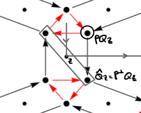
The subspace associated to the unique two outgoing edges at z∈𝒦z\in{\mathcal{K}} is RanQ^z\mathop{\rm Ran}\nolimits\widehat{Q}_{z} with the projection

Q^z:=U​Qz​U∗,\widehat{Q}_{z}:=UQ_{z}U^{\ast},

see figure (2).

Figure 2: The incoming and outgoing projections QzQ_{z} and Q^z\widehat{Q}_{z}
Remark 2.1.

Note that Qz,Q^zQ_{z},\widehat{Q}_{z} do not depend on the collection of scattering matrices.

The basic tool for the discussion of the flux operator is the following proposition which we adapt form [4], proposition 4.2, including its short intuitive proof.

Proposition 2.2.

Let MM be a subset of ℛ{\mathcal{R}} and PP the multiplication operator P=χ⁡(x∈M)P=\chi(x\in M),

Φ=U∗​P​U−P.\Phi=U^{\ast}PU-P.

Then it holds

  1. 1.

    [Φ,Qz]=0∀z∈𝒦\left[\Phi,Q_{z}\right]=0\quad\forall z\in{\mathcal{K}};

  2. 2.

    Φ​Qz=U∗​(P​Q^z)​U−P​Qz\Phi Q_{z}=U^{\ast}(P\widehat{Q}_{z})U-PQ_{z};

  3. 3.

    ind​(Φ)\mbox{ ind}(\Phi) is well defined iff for a c,R>0c,R>0 : sup|z|>R‖Φ​Qz‖≤c<1\sup_{|z|>R}\|\Phi Q_{z}\|\leq c<1; then it holds:

     ind​(Φ)=∑z,|z|≤RdimRan⁡(P​Q^z)−dimRan⁡(P​Qz).\mbox{ ind}(\Phi)=\sum_{z,|z|\leq R}\dim\mathop{\rm Ran}\nolimits(P\widehat{Q}_{z})-\dim\mathop{\rm Ran}\nolimits(PQ_{z}). (1)
Proof.

By definition Qz,Q^zQ_{z},\widehat{Q}_{z} are multiplication operators on ℓ2​(ℛ,ℂ)\ell^{2}({\mathcal{R}};{\mathbb{C}}) thus commute with PP, or

[Φ,Qz]=[U∗​P​U,Qz]=U∗​[P,Q^z]​U=0.[\Phi,Q_{z}]=[U^{\ast}PU,Q_{z}]=U^{\ast}[P,\widehat{Q}_{z}]U=0.

Also ker⁡(Φ2−𝕀)=⨁z∈𝒦ker⁡((Φ2−𝕀)​Qz)\ker\left(\Phi^{2}-{\mathbb{I}}\right)=\bigoplus_{z\in{\mathcal{K}}}\ker\left((\Phi^{2}-{\mathbb{I}})Q_{z}\right) and σ⁡(Φ2)=⋃z∈𝒦σ⁡(Φ2​Qz)\sigma\left(\Phi^{2}\right)=\bigcup_{z\in{\mathcal{K}}}\sigma\left(\Phi^{2}Q_{z}\right). By assumption d​i​s​t​({1},⋃|z|>Rσ⁡(Φ2​Qz))>0dist\left(\{1\},\bigcup_{|z|>R}\sigma(\Phi^{2}Q_{z})\right)>0 thus 11 is an isolated finite dimensional eigenvalue and

 ind​(Φ)=∑|z|≤Rdimker⁡((Φ−𝕀)​Qz)−∑|z|≤Rdimker⁡((Φ+𝕀)​Qz)=\mbox{ ind}(\Phi)=\sum_{|z|\leq R}\dim\ker\left((\Phi-{\mathbb{I}})Q_{z}\right)-\sum_{|z|\leq R}\dim\ker\left((\Phi+{\mathbb{I}})Q_{z}\right)=
=∑|z|≤R ind​(Φ​Qz)=∑|z|≤Rt​r​a​c​e​(Φ​Qz)=∑z,|z|≤RdimRan⁡(P​Q^z)−dimRan⁡(P​Qz).=\sum_{|z|\leq R}\mbox{ ind}(\Phi Q_{z})=\sum_{|z|\leq R}trace(\Phi Q_{z})=\sum_{z,|z|\leq R}\dim\mathop{\rm Ran}\nolimits(P\widehat{Q}_{z})-\dim\mathop{\rm Ran}\nolimits(PQ_{z}).

∎

In order to efficiently define the projection and to count the relevant dimensions we associate to the family of unitaries UU the directed Ruby graph G=(ℛ,ℰ)G=({\mathcal{R}},{\mathcal{E}}) whose set of vertices is ℛ{\mathcal{R}} and whose directed edges ℰ{\mathcal{E}} are defined by, c.f. figure (4),

x​y→∈ℰ​ iff ​⟨y,Uc​x⟩≠0\overrightarrow{xy}\in{\mathcal{E}}\hbox{ \it iff }\langle y,U_{c}\ x\rangle\neq 0

where UcU_{c} is the model which has all its scattering matrices Sz=12​(1−111)S_{z}=\frac{1}{\sqrt{2}}\left(\begin{array}[]{cc}1&-1\\ 1&1\end{array}\right).

For a given UU we attribute

 the weight ​|⟨y,U​x⟩|​ to the edge ​x​y→∈ℰ.\hbox{ the weight }|\langle y,Ux\rangle|\hbox{ to the edge }\overrightarrow{xy}\in{\mathcal{E}}.

For a given z∈𝒦z\in{\mathcal{K}} there are four edges, we label the weight by |rz||r_{z}| (color: black) if the corresponding current is scattered to its left and by |tz||t_{z}| if it is scattered to its right (color: red). Explicitly we have for z∈𝒦1z\in{\mathcal{K}}_{1}

|⟨z−14v2,U(z+14v1)⟩|=:|tz|,|⟨z+14v2,U(z+14v1)⟩|=:|rz|\left|\left\langle z-\frac{1}{4}v_{2},U(z+\frac{1}{4}v_{1})\right\rangle\right|=:\left|t_{z}\right|,\qquad\left|\left\langle z+\frac{1}{4}v_{2},U(z+\frac{1}{4}v_{1})\right\rangle\right|=:|r_{z}|

and all other cases analogously, see figure (3).

Remark that for a choice of a basis in each RanQz,RanQ^z\mathop{\rm Ran}\nolimits Q_{z},\mathop{\rm Ran}\nolimits\widehat{Q}_{z} which is compatible with this convention, the parameters are

Sz≡qz​(rz−tztz¯rz¯) with ​qz∈S1,rz,tz∈ℂ​ s.t. ​|rz|2+|tz|2=1.S_{z}\equiv q_{z}\left(\begin{array}[]{cc}r_{z}&-t_{z}\\ \bar{t_{z}}&\bar{r_{z}}\end{array}\right)\quad\hbox{ with }q_{z}\in S^{1},r_{z},t_{z}\in{\mathbb{C}}\hbox{ s.t. }|r_{z}|^{2}+|t_{z}|^{2}=1.

Figure 3: The weights of (ℛ,ℰ)({\mathcal{R}},{\mathcal{E}}).

The projection PP will be defined by a path in the dual graph.

The faces of the Ruby graph figure (4) which are adjacent to a fixed vertex are in turn a triangle, a rectangle, a hexagon, a rectangle. The dual graph

G∗=(ℛ∗,ℰ∗)G^{\ast}=({\mathcal{R}}^{\ast},{\mathcal{E}}^{\ast})

has its vertices at the center of the faces of (ℛ,ℰ)({\mathcal{R}},{\mathcal{E}}) and the dual edges (which we call links to distinguish) are segments which connect to all next neighbors thus bisecting edges of ℰ{\mathcal{E}}. Remark that the scattering points are the centers of the rectangles in the Ruby graph: 𝒦⊂ℛ∗{\mathcal{K}}\subset{\mathcal{R}}^{\ast}.

Figure 4: The Ruby graph

Figure 5: An admissible path defining the projection on the states on its left

Now consider a partition of GG in two infinite connected subgraphs G+G_{+} and G−G_{-}, consider a path in G∗G^{\ast} which bisects the edge boundary of G+G_{+} and visualize this path as an injective, continuous, and piecewise unit speed curve of straight segments on the dual graph in ℝ2{\mathbb{R}}^{2}

γ:ℝ→G∗⊂ℝ2​ such that for integer ​t∈ℤ:γ⁡(t)∈ℛ∗​ and ​γ⁡(t)​γ​(t+1)→∈ℰ∗\gamma:{\mathbb{R}}\to G^{\ast}\subset{\mathbb{R}}^{2}\hbox{ such that for integer }t\in{\mathbb{Z}}:\gamma(t)\in{\mathcal{R}}^{\ast}\hbox{ and }\overrightarrow{\gamma(t)\gamma(t+1)}\in{\mathcal{E}}^{\ast}

oriented such that G+G_{+} is to the left of γ\gamma; we call it an admissible path, see figure (5). Let ℛ+{\mathcal{R}}_{+} be the set of vertices of G+G_{+} and consider its projection and flux operator in ℓ2​(ℛ,ℂ)\ell^{2}({\mathcal{R}};{\mathbb{C}}) :

Pγ=χ⁡(x∈ℛ+),Φγ=U∗​Pγ​U−Pγ.P_{\gamma}=\chi(x\in{\mathcal{R}}_{+}),\quad\Phi_{\gamma}=U^{\ast}P_{\gamma}U-P_{\gamma}.

In the following we shall give sufficient conditions for non trivial  ind​(Φγ)\mbox{ ind}(\Phi_{\gamma}). By the general theory of Theorem A.1 and Proposition A.2 we know that all vertices which are not incident to the edge boundary of G+G_{+} belong to ker⁡(Φγ)\ker(\Phi_{\gamma}); in view of the basic formula (1) we label the set of interesting vertices as follows:

Definition 2.3.

Let γ:ℝ→G∗\gamma:{\mathbb{R}}\to G^{\ast} be an admissible path. We call ℰγ⊂ℰ{\mathcal{E}}_{\gamma}\subset{\mathcal{E}} the set of edges bisected by γ\gamma and 𝒦γ{\mathcal{K}}_{\gamma} the labels of subspaces RanQz\mathop{\rm Ran}\nolimits Q_{z} which contain vertices incident to ℰγ{\mathcal{E}}_{\gamma}, i.e. :

𝒦γ:={z∈𝒦;Pγ⟂UcPγQz≠0 or PγUcPγ⟂Qz≠0}.{\mathcal{K}}_{\gamma}:=\left\{z\in{\mathcal{K}};P_{\gamma}^{\perp}U_{c}P_{\gamma}Q_{z}\neq 0\hbox{ or }P_{\gamma}U_{c}P_{\gamma}^{\perp}Q_{z}\neq 0\right\}.

From this graphical representation of UU and PP we can literally read off how to construct a useful admissible path. The basis observation is:

Remark 2.4.

From equation (1) and the fact that QzQ_{z} and Q^z\widehat{Q}_{z} are diagonally opposite vertices of the rectangles of the Ruby graph, we observe: consecutively bisected links of type hexagon-rectangle-hexagons as well as triangle-rectangle-triangle do not contribute to the index because at the common dual vertex z∈𝒦z\in{\mathcal{K}} it holds dimRan⁡P​Qz=dimRan⁡P​Q^z\dim\mathop{\rm Ran}\nolimits PQ_{z}=\dim\mathop{\rm Ran}\nolimits P\widehat{Q}_{z}. On the other hand consecutively bisected links of type hexagon-rectangle-triangle as well as triangle-rectangle-hexagon do contribute to the index because dimRan⁡P​Qz≠dimRan⁡P​Q^z\dim\mathop{\rm Ran}\nolimits PQ_{z}\neq\dim\mathop{\rm Ran}\nolimits P\widehat{Q}_{z}, see figure (6).

We define the non contributing parts :

Definition 2.5.

Let I⊂ℝI\subset{\mathbb{R}}. An admissible path γ\gamma is called a rr-path in I⊂ℝI\subset{\mathbb{R}} if its restriction to II bisects only edges of weight |r||r| and a tt-path in I⊂ℝI\subset{\mathbb{R}} if its restriction to II bisects only edges of weight |t||t|.

Concerning the regularity of Φγ\Phi_{\gamma} we have

Refer to caption
(a) r and r edge
Refer to caption
(b) t and t edge
Refer to caption
(c) outgoing r and t edge
Figure 6: Parts contributing and non contributing to  ind​(Φ)\mbox{ ind}(\Phi)
Lemma 2.6.

Let γ\gamma be an admissible rr-path in ℝ{\mathbb{R}}; then it holds for the operator and the trace norm:

‖Φγ‖≤supz∈𝒦γ|rz|,‖Φγ‖1≤c​o​n​s​t.∑z∈𝒦γ|rz|.\|\Phi_{\gamma}\|\leq\sup_{z\in{\mathcal{K}}_{\gamma}}|r_{z}|,\quad\|\Phi_{\gamma}\|_{1}\leq const.\sum_{z\in{\mathcal{K}}_{\gamma}}|r_{z}|.

The analogous statement holds true for a tt-path

Proof.

Only states with label in 𝒦γ{\mathcal{K}}_{\gamma} contribute, by Theorem A.2.1: [Φγ2,Qz]=0[\Phi_{\gamma}^{2},Q_{z}]=0 and γ\gamma crosses only edges of weight |rz||r_{z}| thus Φγ2​Qz=|rz|2​Qz\Phi_{\gamma}^{2}Q_{z}=|r_{z}|^{2}Q_{z}, see figure (7), so we have

Φγ2=P​U∗​Pγ⟂​U​Pγ+Pγ⟂​U∗​Pγ​U​Pγ⟂=∑z∈𝒦Φγ2​Qz=∑z∈𝒦γΦγ2​Qz=∑z∈𝒦γ|rz|2​Qz.\Phi_{\gamma}^{2}=PU^{\ast}P_{\gamma}^{\perp}UP_{\gamma}+P_{\gamma}^{\perp}U^{\ast}P_{\gamma}UP_{\gamma}^{\perp}=\sum_{z\in{\mathcal{K}}}\Phi_{\gamma}^{2}Q_{z}=\sum_{z\in{\mathcal{K}}_{\gamma}}\Phi_{\gamma}^{2}Q_{z}=\sum_{z\in{\mathcal{K}}_{\gamma}}|r_{z}|^{2}Q_{z}.

. It follows that |Φγ|=∑z∈𝒦γ|rz|​Qz|\Phi_{\gamma}|=\sum_{z\in{\mathcal{K}}_{\gamma}}|r_{z}|Q_{z} which implies the assertion.

Figure 7: The action of Φ2​Qz\Phi^{2}Q_{z} for an rr-path

∎

We are now able to prove that a Chalker Coddington model on the Ruby graph which admits a suitable admissible path defines a projection with non-trivial flux. We show that a path is suitable if it crosses only hexagons and rectangles in the past and only triangles and rectangles in the future, and such that the associated weights are sufficiently regular. Remark that an analogous result was proved in Theorem 4.7 in [4] for the L-network which leads to the original Chalker Coddington model on the associated Manhattan graph. We can adapt this result without essential difficulty to the present situation.

Theorem 2.7.

Let UU be a Chalker Coddington model on the Ruby graph such that there exists an admissible path γ\gamma which is an rr-path in (−∞,−N](-\infty,-N] and a tt-path in [N,∞)[N,\infty) for an integer N>1N>1, and such that for a c>0c>0

|rz|≤c<1∀z∈𝒦γ↾(−∞,−N] and |tz|≤c<1∀z∈𝒦γ↾[N,∞).|r_{z}|\leq c<1\quad\forall z\in{\mathcal{K}}_{\gamma\restriction(-\infty,-N]}\hbox{ and }|t_{z}|\leq c<1\quad\forall z\in{\mathcal{K}}_{\gamma\restriction[N,\infty)}.

Then  ind​(Φγ)\mbox{ ind}(\Phi_{\gamma}) is well defined and it holds

| ind​(Φγ)|=1.|\mbox{ ind}(\Phi_{\gamma})|=1.

In addition

  1. 1.

    Φγ\Phi_{\gamma} is compact iff  lims→−∞rγ⁡(s)=0=lims→∞tγ⁡(s)\lim_{s\to-\infty}{r_{\gamma(s)}}=0=\lim_{s\to\infty}{t_{\gamma(s)}} and then

    σ⁡(U)=S1.\sigma(U)=S^{1}.
  2. 2.

    Φγ\Phi_{\gamma} is trace class iff  ∑z∈𝒦γ↾(−∞,−N]|rz|+∑z∈𝒦γ↾[N,∞)|tz|<∞\sum_{z\in{\mathcal{K}}_{\gamma\restriction(-\infty,-N]}}|r_{z}|+\sum_{z\in{\mathcal{K}}_{\gamma\restriction[N,\infty)}}|t_{z}|<\infty and then

    σa​c​(U)=S1,\sigma_{ac}(U)=S^{1},

    and a trace class perturbation of UU contains a shift operator.

Proof.

If γ\gamma is a path which switches from rr to tt on one site, i.e : if γ\gamma is an rr-path in (−∞,0)(-\infty,0) and a tt-path in [0,∞)[0,\infty), then as a corollary of Proposition 2.2 and Remark 2.4 we have

 ind(Φ)=∑z∈𝒦γ↾[−N,N]dimRan(PQ^z)−dimRan(PQz)=dimRan(PQ^z0)−dimRan(PQz0)\mbox{ ind}(\Phi)=\sum_{z\in{\mathcal{K}}_{\gamma\restriction_{[-N,N]}}}\dim\mathop{\rm Ran}\nolimits(P\widehat{Q}_{z})-\dim\mathop{\rm Ran}\nolimits(PQ_{z})=\dim\mathop{\rm Ran}\nolimits(P\widehat{Q}_{z_{0}})-\dim\mathop{\rm Ran}\nolimits(PQ_{z_{0}})

with z0=γ⁡(0)z_{0}=\gamma(0). By the symmetry of the problem the two edges bisected by the links adjacent to γ⁡(0)\gamma(0) are either incoming or outgoing to G+G_{+} thus dimRan⁡P​Qz0=1\dim\mathop{\rm Ran}\nolimits PQ_{z_{0}}=1 and dimRan⁡P​Q^z0=0\dim\mathop{\rm Ran}\nolimits P\widehat{Q}_{z_{0}}=0 or the other way round, see figure (6(c)). Thus | ind​(Φγ)|=1|\mbox{ ind}(\Phi_{\gamma})|=1.

If γ\gamma switches several times cutting rr and tt links then choose two integers N±∈ℤN_{\pm}\in{\mathbb{Z}} such that ±N±>±N\pm N_{\pm}>\pm N and such that γ⁡(N−)\gamma(N_{-}) is the center of a hexagon and γ⁡(N+)\gamma(N_{+}) the center of a triangle. Thus all links incident to γ⁡(N−)\gamma(N_{-}) bisect edges of weight |r||r| and all links incident to γ⁡(N+)\gamma(N_{+}) bisect edges of weight |t||t|. Then we can define a new admissible path γ^\widehat{\gamma} replacing the part γ↾(−N−,N+)\gamma\restriction_{(-N_{-},N_{+})} by an rr path inside G+G_{+} connecting γ⁡(N−)\gamma(N_{-}) to γ⁡(N+)\gamma(N_{+}), c.f. figure (8). The new path switches from rr to tt only at γ⁡(N+)\gamma(N_{+}).The difference Pγ−Pγ^P_{\gamma}-P_{\widehat{\gamma}} is of finite rank thus by the invariance properties of the index

 ind​(Φγ)= ind​(Φγ^).\mbox{ ind}(\Phi_{\gamma})=\mbox{ ind}(\Phi_{\widehat{\gamma}}).

The additional assertions follow from Lemma 2.6 and Theorem A.1.

Figure 8: Join r path to t path in figure (5)

∎

As by unitarity we have |rz|2+|tz|2=1|r_{z}|^{2}+|t_{z}|^{2}=1 it follows:

Corollary 2.8.

Any Chalker Coddington model on the Ruby graph defined by a collection of scattering matrices such that for c1,c2∈(0,1)c_{1},c_{2}\in(0,1) and all zz: 0<c1<|rz|<c2<10<c_{1}<|r_{z}|<c_{2}<1, admits a projection with non trivial index.

Remark 2.9.

A remarkable situation which is covered by the Corollary is the translation invariant 0<|rz|=c​o​n​s​t≠10<|r_{z}|=const\neq 1 case with all phases equal to unity; here the spectrum is absolutely continuous and exhibits gaps or not. However, for a γ\gamma with a r−tr-t transition the flux operator Φγ\Phi_{\gamma} is not trace class or even compact. The analogous situation is present for perturbations of the translation invariant model, see [2].

3 Edge current in two dimensional spin-1/21/2 Quantum Walks

We analyze transport properties of a class of two dimensional spin-1/21/2 Quantum Walks proposed in [14] for which transport seems to have been experimentally observed [10]. The feature of these walks is that they depend on two ℂ2{\mathbb{C}}^{2} coins. We use the methods which were developed in [4] for coined Quantum Walks which depend on one ℂ4{\mathbb{C}}^{4} coin and analyze the flux out of a subspace defined by a projection which can be interpreted as a quantum lead.

We present the class of models. The Hilbert space is ℍ=ℓ2​(ℤ2,ℂ2){\mathbb{H}}=\ell^{2}({\mathbb{Z}}^{2};{\mathbb{C}}^{2}) its canonical scalar product ⟨⋅,⋅⟩\left\langle\cdot,\cdot\right\rangle.

For a family of 2×22\times 2 matrices {M⁡(z)}z∈ℤ2⊂𝕄⁡(2,ℂ)\{M(z)\}_{z\in{\mathbb{Z}}^{2}}\subset{\mathbb{M}}(2;{\mathbb{C}}) the multiplication operator 𝐌{\bf M} on ℍ{\mathbb{H}} with symbol MM is

𝐌​ψ​(z):=M⁡(z)​ψ​(z),ψ∈ℍ.{\bf M}\psi(z):=M(z)\psi(z),\quad\psi\in{\mathbb{H}}.

A coin 𝐂{\bf C} is a multiplication operator with unitary symbol {C⁡(z)}z∈ℤ2⊂U⁡(2)\{C(z)\}_{z\in{\mathbb{Z}}^{2}}\subset U(2).

With the canonical basis vectors, ex,eye_{x},e_{y} of ℤ2{\mathbb{Z}}^{2} denote Sj​ψ​(z):=ψ⁡(z−ej),j∈{x,y}S_{j}\psi(z):=\psi(z-e_{j}),\quad j\in\{x,y\} the shift in the xx or yy direction. The corresponding conditional shifts are

𝐓j:ℍ→ℍ,𝐓j​ψ​(z):=(Sj00Sj∗)​ψ​(z)=(ψ1​(z−ej)ψ2​(z+ej)).{\bf T}_{j}:{\mathbb{H}}\to{\mathbb{H}},\quad{\bf T}_{j}\psi(z):=\left(\begin{array}[]{cc}S_{j}&0\\ 0&S_{j}^{\ast}\end{array}\right)\psi(z)=\left(\begin{array}[]{c}\psi_{1}(z-e_{j})\\ \psi_{2}(z+e_{j})\end{array}\right).

We use the expressions 𝐓j=Sj​𝐏++Sj∗​𝐏−{\bf T}_{j}=S_{j}{\bf P}_{+}+S_{j}^{\ast}{\bf P}_{-} with the projections 𝐏±{\bf P}_{\pm} whose symbols are {P±}z∈ℤ2\{P_{\pm}\}_{z\in{\mathbb{Z}}^{2}} the projections on the upper resp. lower component of ℂ2{\mathbb{C}}^{2}. We also use ℤ2∋z=(x,y){\mathbb{Z}}^{2}\ni z=(x,y) and denote the canonical basis vectors of ℍ{\mathbb{H}} by

|z0;+⟩:=(ℤ2∋z↦δz,z0​(10)∈ℂ2),|z0;−⟩:=(ℤ2∋z↦δz,z0​(01)∈ℂ2).\Ket{z_{0};+}:=\left({\mathbb{Z}}^{2}\ni z\mapsto\delta_{z,z_{0}}\left(\begin{array}[]{c}1\\ 0\end{array}\right)\in{\mathbb{C}}^{2}\right),\quad\Ket{z_{0};-}:=\left({\mathbb{Z}}^{2}\ni z\mapsto\delta_{z,z_{0}}\left(\begin{array}[]{c}0\\ 1\end{array}\right)\in{\mathbb{C}}^{2}\right).

Note that Sj​|z;±⟩=|z+ej;±⟩S_{j}\Ket{z;\pm}=\Ket{z+e_{j};\pm}.

The family of unitary operators which we study depends parametrically on two unitary symbols:

Let 𝐂1,𝐂2{\bf C}_{1},{\bf C}_{2} two coins. Define

U:ℍ→ℍ,U:=𝐓y​C2​𝐓x​C1.U:{\mathbb{H}}\to{\mathbb{H}},\qquad U:={\bf T}_{y}C_{2}{\bf T}_{x}C_{1}. (2)

In order to fix notations, we parametrize the symbols for z∈ℤ2z\in{\mathbb{Z}}^{2} by

Cj​(z)=qj​(z)​(rj​(z)−tj​(z)tj¯​(z)rj¯​(z))​ with ​q​(z)∈S1,r⁡(z),t⁡(z)∈ℂ​ s.t. ​|r⁡(z)|2+|t⁡(z)|2=1.C_{j}(z)=q_{j}(z)\left(\begin{array}[]{cc}r_{j}(z)&-t_{j}(z)\\ \overline{t_{j}}(z)&\overline{r_{j}}(z)\end{array}\right)\hbox{ with }q(z)\in S^{1},r(z),t(z)\in{\mathbb{C}}\hbox{ s.t. }|r(z)|^{2}+|t(z)|^{2}=1.

To illustrate the action of UU, see figure (9), we use the kernel U⁡(⋅,⋅):ℤ2×ℤ2→𝕄⁡(2,ℂ)U(\cdot,\cdot):{\mathbb{Z}}^{2}\times{\mathbb{Z}}^{2}\to{\mathbb{M}}(2;{\mathbb{C}}) such that (U​ψ)​(z)=∑w∈ℤ2U⁡(z,w)​ψ​(w)(U\psi)(z)=\sum_{w\in{\mathbb{Z}}^{2}}U(z,w)\psi(w) which is

U⁡(z,w)={(q2​r2)​(w+ex)​q1​(w)​(r1​(w)−t1​(w)00) if ​z=w+ex+ey(q2​r2¯)​(w−ex)​q1​(w)​(00t1¯​(w)r1¯​(w)) if ​z=w−ex−ey(−q2​t2)​(w−ex)​q1​(w)​(t1¯​(w)r1¯​(w)00) if ​z=w−ex+ey(q2​t2¯)​(w+ex)​q1​(w)​(00r1​(w)−t1​(w)) if ​z=w+ex−ey(0000) elsewhere U(z,w)=\left\{\begin{array}[]{ll}(q_{2}r_{2})(w+e_{x})q_{1}(w)\left(\begin{array}[]{cc}r_{1}(w)&-t_{1}(w)\\ 0&0\end{array}\right)&\hbox{ if }z=w+e_{x}+e_{y}\\ (q_{2}\overline{r_{2}})(w-e_{x})q_{1}(w)\left(\begin{array}[]{cc}0&0\\ \overline{t_{1}}(w)&\overline{r_{1}}(w)\end{array}\right)&\hbox{ if }z=w-e_{x}-e_{y}\\ (-q_{2}t_{2})(w-e_{x})q_{1}(w)\left(\begin{array}[]{cc}\overline{t_{1}}(w)&\overline{r_{1}}(w)\\ 0&0\end{array}\right)&\hbox{ if }z=w-e_{x}+e_{y}\\ (q_{2}\overline{t_{2}})(w+e_{x})q_{1}(w)\left(\begin{array}[]{cc}0&0\\ {r_{1}}(w)&-{t_{1}}(w)\end{array}\right)&\hbox{ if }z=w+e_{x}-e_{y}\\ \left(\begin{array}[]{cc}0&0\\ 0&0\end{array}\right)&\hbox{ elsewhere }\end{array}\right.

Figure 9: The action of UU with the identifications r1↔|q1​r1|r_{1}\leftrightarrow|q_{1}r_{1}|
and r2↔|q2r2(⋅±ex)|…r_{2}\leftrightarrow|q_{2}r_{2}(\cdot\pm e_{x})|\ldots

The basic observation is:

Proposition 3.1.

Let 𝐂1.𝐂2{\bf C}_{1}.{\bf C}_{2} be two coins such that

r2​(x,0)=0=t1​(x,0)x∈ℤt2​(x,−1)=0=r1​(x,−1)x∈ℤ.\left.\begin{array}[]{ll}r_{2}(x,\phantom{-}0)=0=t_{1}(x,\phantom{-}0)&x\in{\mathbb{Z}}\\ t_{2}(x,-1)=0=r_{1}(x,-1)&x\in{\mathbb{Z}}\end{array}\right..

Then for U=𝐓y​𝐂2​𝐓x​𝐂1U={\bf T}_{y}{\bf C}_{2}{\bf T}_{x}{\bf C}_{1} the subspace

ℍ0:=⨁x∈ℤs​p​a​n​{|x,0;+⟩,|x,−1;−⟩}{\mathbb{H}}_{0}:=\bigoplus_{x\in{\mathbb{Z}}}span\left\{\Ket{x,0;+},\Ket{x,-1;-}\right\}

is invariant for UU. Furthermore U↾ℍ0U\restriction{\mathbb{H}}_{0} is a two dimensional shift with wandering subspace 𝕃0:=s​p​a​n​{|−1,0;+⟩,|−1,−1;−⟩}{\mathbb{L}}_{0}:=span\left\{\Ket{-1,0;+},\Ket{-1,-1;-}\right\}, i.e. Un​𝕃0⟂𝕃0,∀n≠0U^{n}{\mathbb{L}}_{0}\perp{\mathbb{L}}_{0},\quad\forall n\neq 0 and ⨁n∈ℤUn​𝕃0=ℍ0\bigoplus_{n\in{\mathbb{Z}}}U^{n}{\mathbb{L}}_{0}={\mathbb{H}}_{0}

Proof.

The proof is by explicit calculation which we present for

C2​(x,0)=(0110),C1​(x,0)=(1001),C_{2}(x,0)=\left(\begin{array}[]{cc}0&1\\ 1&0\end{array}\right),\qquad C_{1}(x,0)=\left(\begin{array}[]{cc}1&0\\ 0&1\end{array}\right),
C2​(x,−1)=(1001),C1​(x,−1)=(0110),C_{2}(x,-1)=\left(\begin{array}[]{cc}1&0\\ 0&1\end{array}\right),\qquad C_{1}(x,-1)=\left(\begin{array}[]{cc}0&1\\ 1&0\end{array}\right),

because for the general case all the phases which may appear eventually cancel for the projections below. We have for x∈ℤx\in{\mathbb{Z}}

|x,0;+⟩→𝐂1|x,0;+⟩→𝐓x|x+1,0;+⟩→𝐂2|x+1,0;−⟩→𝐓y|x+1,−1;−⟩​ and \Ket{x,0;+}\xrightarrow{{\bf C}_{1}}\Ket{x,0;+}\xrightarrow{{\bf T}_{x}}\Ket{x+1,0;+}\xrightarrow{{\bf C}_{2}}\Ket{x+1,0;-}\xrightarrow{{\bf T}_{y}}\Ket{x+1,-1;-}\hbox{ and }
|x,−1;−⟩→𝐂1|x,−1;+⟩→𝐓x|x+1,−1;+⟩→𝐂2|x+1,−1;+⟩→𝐓y|x+1,0;+⟩\Ket{x,-1;-}\xrightarrow{{\bf C}_{1}}\Ket{x,-1;+}\xrightarrow{{\bf T}_{x}}\Ket{x+1,-1;+}\xrightarrow{{\bf C}_{2}}\Ket{x+1,-1;+}\xrightarrow{{\bf T}_{y}}\Ket{x+1,0;+}

and thus it holds for the projections in these directions

U​|x,0;+⟩​⟨x,0;+|​U∗=|x+1,−1;−⟩​⟨x+1,−1;−|​ and U\Ket{x,0;+}\bra{x,0;+}U^{\ast}=\Ket{x+1,-1;-}\Bra{x+1,-1;-}\hbox{ and }
U​|x,−1;−⟩​⟨x,−1;−|​U∗=|x+1,0;+⟩​⟨x+1,0;+|.U\Ket{x,-1;-}\Bra{x,-1;-}U^{\ast}=\Ket{x+1,0;+}\Bra{x+1,0;+}.

By induction and unitarity this implies for n∈ℤn\in{\mathbb{Z}}

Un​(|0,0;+⟩​⟨0,0;+|+|0,−1;−⟩​⟨0,−1;−|)​U∗n=|n,0;+⟩​⟨n,0;+|+|n,−1;−⟩​⟨n,−1;−|U^{n}\left(\Ket{0,0;+}\bra{0,0;+}+\Ket{0,-1;-}\Bra{0,-1;-}\right){U^{\ast}}^{n}=\Ket{n,0;+}\Bra{n,0;+}+\Ket{n,-1;-}\Bra{n,-1;-}

which proves the three assertions. ∎

Remark 3.2.

Remark that under the conditions of proposition 3.1 the absolutely continuous spectrum of UU is the full unit circle but other types of spectra of UU typically coexist because: σa​c​(U↾ℍ0)=S1⊂σa​c​(U)\sigma_{ac}(U\restriction{\mathbb{H}}_{0})=S^{1}\subset\sigma_{ac}(U) and the coins 𝐂1,𝐂2{\bf C}_{1},{\bf C}_{2} are arbitrary on ℍ0⟂{\mathbb{H}}_{0}^{\perp}.

Now making use of the theory of the index of two projections and its topological invariance we can substantially extend this to a precise result on the existence of a current which was observed in the experiment of [10]. We consider the projection on a two state quantum half line, i.e.:

Definition 3.3.

Let 𝐏{\bf P} be the projection valued multiplication operator with symbol PP defined by

P⁡(x):={P+x≥0​ and ​y=0P−x≥0​ and ​y=−10elsewhere.P(x):=\left\{\begin{array}[]{ll}P_{+}&x\geq 0\hbox{ and }y=0\\ P_{-}&x\geq 0\hbox{ and }y=-1\\ 0&\hbox{elsewhere}\end{array}\right.. (3)

It is a corollary of Proposition 3.1 that 𝕃0{\mathbb{L}}_{0} is the incoming subspace for RanP\mathop{\rm Ran}\nolimits P:

Remark 3.4.

UU defined in Proposition 3.1 is a forward shift in RanP\mathop{\rm Ran}\nolimits P, Un​𝕃0⟂𝕃0,∀n∈ℕU^{n}{\mathbb{L}}_{0}\perp{\mathbb{L}}_{0},\forall n\in{\mathbb{N}} and RanP=⨁n∈ℕUn​𝕃0\mathop{\rm Ran}\nolimits P=\bigoplus_{n\in{\mathbb{N}}}U^{n}{\mathbb{L}}_{0}.

This existence of a current holds true for a large class of UU in the following precise sense:

Theorem 3.5.

Let 𝐂1.𝐂2{\bf C}_{1}.{\bf C}_{2} be two coins such that

∑x∈ℕ(|r2​(x,0)|+|t1​(x,0)|+|t2​(x,−1)|+|r1​(x,−1)|)<∞\sum_{x\in{\mathbb{N}}}\left(\left|r_{2}(x,0)\right|+\left|t_{1}(x,0)\right|+\left|t_{2}(x,-1)\right|+\left|r_{1}(x,-1)\right|\right)<\infty

then it holds for UU defined in (2), PP in (3) and Φ:=U∗​P​U−P\Phi:=U^{\ast}PU-P:

Φ​ is trace class with  ind​(Φ)=2,\Phi\hbox{ is trace class with }\mbox{ ind}(\Phi)=2,
σa​c​(U)=S1,\sigma_{ac}(U)=S^{1},

and there exist a unitary trace class perturbation U^=S⊕U~\widehat{U}=S\oplus\widetilde{U} of UU with SS a bilateral shift of multiplicity 22; further there exists a 22 dimensional subspace

𝕃⊂kerP⟂UP⟂↾RanP⟂{\mathbb{L}}\subset\ker P^{\perp}UP^{\perp}\restriction_{\mathop{\rm Ran}\nolimits P^{\perp}}

such that

Sn𝕃⟂𝕃,∀ℤ∋n≠0andSn𝕃=PSn𝕃,∀n∈ℕ.S^{n}{\mathbb{L}}\perp{\mathbb{L}},\forall{\mathbb{Z}}\ni n\neq 0\quad\hbox{and}\quad S^{n}{\mathbb{L}}=PS^{n}{\mathbb{L}},\forall n\in{\mathbb{N}}.
Proof.

Separating the phases we write for the parameters of 𝐂1,𝐂2{\bf C}_{1},{\bf C}_{2}: rj=ei​ρj​|rj|=ei​ρj​1−|tj|2r_{j}=e^{i\rho_{j}}|r_{j}|=e^{i\rho_{j}}\sqrt{1-|t_{j}|^{2}} and tj=ei​τj​|tj|=ei​τj​1−|rj|2t_{j}=e^{i\tau_{j}}|t_{j}|=e^{i\tau_{j}}\sqrt{1-|r_{j}|^{2}}.

Define two coins 𝐂10,𝐂20{\bf C}_{1}^{0},{\bf C}_{2}^{0} by the symbols

C20​(z):={q2​(0−ei​τ2e−i​τ20)​(z) if ​z=(x,0),∀x∈ℕq2​(ei​ρ200e−i​ρ2)​(z) if ​z=(x,−1),∀x∈ℕC2​(z) elsewhere ,C_{2}^{0}(z):=\left\{\begin{array}[]{ll}q_{2}\left(\begin{array}[]{cc}0&-e^{i\tau_{2}}\\ e^{-i\tau_{2}}&0\end{array}\right)(z)&\hbox{ if }z=(x,0),\forall x\in{\mathbb{N}}\\ q_{2}\left(\begin{array}[]{cc}e^{i\rho_{2}}&0\\ 0&e^{-i\rho_{2}}\end{array}\right)(z)&\hbox{ if }z=(x,-1),\forall x\in{\mathbb{N}}\\ C_{2}(z)&\hbox{ elsewhere }\end{array},\right.
C10​(z):={q1​(ei​ρ100e−i​ρ1)​(z) if ​z=(x,0),∀x∈ℕq1​(0−ei​τ1e−i​τ10)​(z) if ​z=(x,−1),∀x∈ℕC1​(z) elsewhere .C_{1}^{0}(z):=\left\{\begin{array}[]{ll}q_{1}\left(\begin{array}[]{cc}e^{i\rho_{1}}&0\\ 0&e^{-i\rho_{1}}\end{array}\right)(z)&\hbox{ if }z=(x,0),\forall x\in{\mathbb{N}}\\ q_{1}\left(\begin{array}[]{cc}0&-e^{i\tau_{1}}\\ e^{-i\tau_{1}}&0\end{array}\right)(z)&\hbox{ if }z=(x,-1),\forall x\in{\mathbb{N}}\\ C_{1}(z)&\hbox{ elsewhere }\end{array}.\right.

For the Hilbert-Schmidt norm ∥⋅∥H​S\|\cdot\|_{HS} on 𝕄⁡(2,ℂ){\mathbb{M}}(2;{\mathbb{C}}) we obtain

‖(C2−C20)​(z)‖H​S2≤4​{|r2​(z)|2z=(x,0),∀x∈ℕ|t2​(z)|2z=(x,−1),∀x∈ℕ0elsewhere,\left\|(C_{2}-C_{2}^{0})(z)\right\|_{HS}^{2}\leq 4\left\{\begin{array}[]{ll}|r_{2}(z)|^{2}&z=(x,0),\forall x\in{\mathbb{N}}\\ |t_{2}(z)|^{2}&z=(x,-1),\forall x\in{\mathbb{N}}\\ 0&\hbox{elsewhere}\end{array}\right.,
‖(C1−C10)​(z)‖H​S2≤4​{|t1​(z)|2z=(x,0),∀x∈ℕ|r1​(z)|2z=(x,−1),∀x∈ℕ0elsewhere.\left\|(C_{1}-C_{1}^{0})(z)\right\|_{HS}^{2}\leq 4\left\{\begin{array}[]{ll}|t_{1}(z)|^{2}&z=(x,0),\forall x\in{\mathbb{N}}\\ |r_{1}(z)|^{2}&z=(x,-1),\forall x\in{\mathbb{N}}\\ 0&\hbox{elsewhere}\end{array}\right..

It follows for the trace norm

‖𝐂2−𝐂20‖1+‖𝐂1−𝐂10‖1≤c​o​n​s​t.∑z∈ℤ2∑j‖(Cj−Cj0)​(z)‖H​S≤\displaystyle\|{\bf C}_{2}-{\bf C}_{2}^{0}\|_{1}+\|{\bf C}_{1}-{\bf C}_{1}^{0}\|_{1}\leq const.\sum_{z\in{\mathbb{Z}}^{2}}\sum_{j}\|(C_{j}-C_{j}^{0})(z)\|_{HS}\leq
∑x∈ℕ(|r1​(x,−1)|+|t2​(x,−1)|+|t1​(x,0)|+|r2​(x,0)|)<∞.\displaystyle\sum_{x\in{\mathbb{N}}}\left(\left|r_{1}(x,-1)\right|+\left|t_{2}(x,-1)\right|+\left|t_{1}(x,0)\right|+\left|r_{2}(x,0)\right|\right)<\infty.

For U0:=𝐓y​𝐂20​𝐓x​𝐂10U^{0}:={\bf T}_{y}{\bf C}_{2}^{0}{\bf T}_{x}{\bf C}_{1}^{0}, Φ0:=U0∗​P​U0−P\Phi^{0}:={U^{0}}^{\ast}PU^{0}-P it follows that the difference

U−U0=𝐓y​(𝐂2−𝐂20)​𝐓x​𝐂1+𝐓y​𝐂2​𝐓x​(𝐂1−𝐂10)​ is trace class U-U^{0}={\bf T}_{y}({\bf C}_{2}-{\bf C}_{2}^{0}){\bf T}_{x}{\bf C}_{1}+{\bf T}_{y}{\bf C}_{2}{\bf T}_{x}({\bf C}_{1}-{\bf C}_{1}^{0})\hbox{ is trace class }

and thus

Φ−Φ0​ is trace class .\Phi-\Phi^{0}\hbox{ is trace class }.

Φ0\Phi^{0} equals minus the orthogonal projection on 𝕃0{\mathbb{L}}_{0}. It follows that Φ\Phi is trace class and that  ind​(Φ)=2\mbox{ ind}(\Phi)=2.

Now Theorem A.1.3 and the construction of 𝕃{\mathbb{L}} in its proof (see [4] Theorem 2.1, adapted by replacing P↔P⟂P\leftrightarrow P^{\perp}) implies the assertion. ∎

As an illustration of this result of the existence of a current in the subspace RanP\mathop{\rm Ran}\nolimits P for a trace class perturbation of UU, we explicit the non-triviality of the incoming subspace 𝕃{\mathbb{L}} for UU for a finite rank perturbation of the paradigmatic situation of Proposition 3.1.

Remark 3.6.

Let 𝐂1.𝐂2{\bf C}_{1}.{\bf C}_{2} be two coins such that, c.f. figure (10)

r2​(x,0)=0=t1​(x,0)x∈ℕ∖{1,2}t2​(x,−1)=0=r1​(x,−1)x∈ℕ​⋃{−1,0}.\left.\begin{array}[]{ll}r_{2}(x,\phantom{-}0)=0=t_{1}(x,\phantom{-}0)&x\in{\mathbb{N}}\setminus\{1,2\}\\ t_{2}(x,-1)=0=r_{1}(x,-1)&x\in{\mathbb{N}}\bigcup\{-1,0\}\end{array}\right..

Then for the incoming state 𝕃{\mathbb{L}} of Theorem 3.5 it holds 𝕃:=s​p​a​n​{|−1,−1;−⟩,ψ}{\mathbb{L}}:=span\left\{\Ket{-1,-1;-},\psi\right\} where ψ\psi has generically non zero components on all vectors in {|−1,0;+⟩,|1,0;+⟩,|3,0;+⟩}\{\Ket{-1,0;+},\Ket{1,0;+},\Ket{3,0;+}\}

Figure 10: Illustration of the incoming space for UU in Remark (3.6). The gray dots represent the states in RanP\mathop{\rm Ran}\nolimits P, green arrows the elements of P⟂​U​PP^{\perp}UP, red arrows the incoming elements of P​U​P⟂PUP^{\perp}

Appendix A General results on the flux operator Φ\Phi

The important notion of the relative index of two projections was defined in [5]. We list here some of its known properties which are used above. For the proofs we refer to [5] and [4] as concerns the spectral and dynamical implications.

Theorem A.1.

Let UU be a unitary operator on a Hilbert space and PP an orthogonal projection. For the selfadjoint operator

Φ:=U∗​P​U−P=U∗​[P,U]\Phi:=U^{\ast}PU-P=U^{\ast}\left[P,U\right]

suppose that 11 is an isolated eigenvalue of finite multiplicity of Φ2\Phi^{2} and define the integer

 ind​(Φ):=dimker⁡(Φ−𝕀)−dimker⁡(Φ+𝕀).\mbox{ ind}(\Phi):=\dim\ker\left(\Phi-{\mathbb{I}}\right)-\dim\ker\left(\Phi+{\mathbb{I}}\right).

If the index does not vanish,  ind​(Φ)=n≠0\mbox{ ind}(\Phi)=n\neq 0, then:

there exists a unitary U^\widehat{U} such that U^=S⊕U~\widehat{U}=S\oplus\widetilde{U} where SS is a bilateral shift of multiplicity |n||n|, U~\widetilde{U} is unitary on its subspace , [U~,P]=0[\widetilde{U},P]=0 and :

  1. 1.

    ‖U−U^−F‖=𝒪⁡(‖Φ<‖)\|U-\widehat{U}-F\|={\mathcal{O}}(\|\Phi_{<}\|) for a finite rank operator FF and Φ<\Phi_{<} the restriction of Φ\Phi to its spectral subspace off ±1\pm 1 : Φ<:=Φ​χ​(Φ2<1)\Phi_{<}:=\Phi\chi(\Phi^{2}<1);

  2. 2.

    if [P,U][P,U] is compact then U−U^U-\widehat{U} is compact and the essential spectrum of UU is the whole unit circle :

    σ⁡(U)=S1;\sigma(U)=S^{1};
  3. 3.

    if [P,U][P,U] is trace class then U−U^U-\widehat{U} is trace class and the absolutely continuous spectrum of UU is the whole unit circle:

    σa​c​(U)=S1.\sigma_{ac}(U)=S^{1}.
Proposition A.2.

With Φ\Phi as in Theorem A.1 it holds:

  1. 1.
    Φ2≤1;[Φ2,P]=0;\Phi^{2}\leq 1;\quad[\Phi^{2},P]=0;
    ker⁡(Φ+𝕀)=ker⁡(P​U​P↾RanP);ker⁡(Φ−𝕀)=ker⁡(P⟂​U​P⟂↾RanP⟂).\ker\left(\Phi+{\mathbb{I}}\right)=\ker\left(PUP\restriction\mathop{\rm Ran}\nolimits{P}\right);\quad\ker\left(\Phi-{\mathbb{I}}\right)=\ker\left(P^{\perp}UP^{\perp}\restriction\mathop{\rm Ran}\nolimits{P^{\perp}}\right).
  2. 2.

    If  ind​(Φ)\mbox{ ind}(\Phi) is defined then P​U​PPUP is Fredholm on RanP\mathop{\rm Ran}\nolimits P and  ind​(Φ)\mbox{ ind}(\Phi) equals minus its Fredholm index :

     ind​(Φ)=dimker⁡Q​U∗​Q−dimker⁡Q​U​Q.\mbox{ ind}(\Phi)=\dim\ker QU^{\ast}Q-\dim\ker QUQ.
  3. 3.
     ind​(Φ)=dimker⁡((Φ2−𝕀)↾RanP⟂)−dimker⁡((Φ2−𝕀)↾RanP).\mbox{ ind}(\Phi)=\dim\ker\left((\Phi^{2}-{\mathbb{I}})\restriction\mathop{\rm Ran}\nolimits{P^{\perp}}\right)-\dim\ker\left((\Phi^{2}-{\mathbb{I}})\restriction\mathop{\rm Ran}\nolimits{P}\right).
  4. 4.

    If [0,1]∋t→U⁡(t)[0,1]\ni t\to U(t) is norm continuous and unitary and for Φ⁡(t)=U∗​(t)​P​U​(t)\Phi(t)=U^{\ast}(t)PU(t): 1∉σe​s​s​(Φ​(t)2)1\notin\sigma_{ess}(\Phi(t)^{2}) then ℤ∋ ind​(Φ⁡(t))=c​o​n​s​t.{\mathbb{Z}}\ni\mbox{ ind}(\Phi(t))=const.

  5. 5.

    For unitaries U0U_{0}, U1U_{1} such that U1−U0U_{1}-U_{0} is a compact operator, it holds for the corresponding flux operators Φ0,Φ1\Phi_{0},\Phi_{1}:

     ind​(Φ0)= ind​(Φ1).\mbox{ ind}(\Phi_{0})=\mbox{ ind}(\Phi_{1}).
  6. 6.

    A dd-dimensional subspace 𝕃{\mathbb{L}} is called wandering for a unitary UU, if Uk​𝕃⟂𝕃∀k∈ℕ{{U}}^{k}{\mathbb{L}}\perp{\mathbb{L}}\quad\forall k\in{\mathbb{N}}. For an orthogonal decomposition 𝕃=⨁j=1d𝕃j{\mathbb{L}}=\bigoplus_{j=1}^{d}{\mathbb{L}}_{j} into 1-dimensional subspaces and for the UU-invariant subspace

    𝕄:=⨁k∈ℤUk​𝕃=⨁j=1d⨁k∈ℤUk​𝕃j{\mathbb{M}}:=\bigoplus_{k\in{\mathbb{Z}}}{{U}}^{k}{\mathbb{L}}=\bigoplus_{j=1}^{d}\bigoplus_{k\in{\mathbb{Z}}}{{U}}^{k}{\mathbb{L}}_{j}

    it holds that S:=U↾𝕄S:={U}\restriction{\mathbb{M}} is a bilateral shift of multiplicity dd and U↾𝕄⟂U\restriction{\mathbb{M}}^{\perp} is unitary on 𝕄⟂{\mathbb{M}}^{\perp}. In particular σa​c​(U)=𝕊1\sigma_{ac}(U)={\mathbb{S}}^{1}.

Acknowledgments

This article is part of the requirements for the doctoral thesis of Mohamed Mouneime.

References

  • [1] Asch, J., Bourget, O., Joye, A., Localization Properties of the Chalker-Coddington Model. Ann. H. Poincaré, 11, 1341–1373, (2010).
  • [2] Asch, J., Bourget, O., Joye, A., Spectral Stability of Unitary Network Models, Rev. Math. Phys., 27, 1530004, (2015).
  • [3] Asch, J., Bourget, O., Joye, A., Chirality induced Interface Currents in the Chalker Coddington Model, Journal of Spectral Theory, to appear (2019).
  • [4] Asch, J., Bourget, O., Joye, A., Engineering stable quantum currents at bulk boundaries, submitted, arXiv:1906.08181 [math-ph](2019)
  • [5] Avron, J., Seiler, R., Simon, B., The Index of a Pair of Projections, J. Func. Anal., 120, 220-237, (1994)
  • [6] Cedzich, C., Geib, T., Grünbaum, F. A., Stahl, C., Velázquez, L., Werner, A. H., Werner, R. F., The topological classification of one-dimensional symmetric quantum walks. Ann. H. Poincaré, 19, 325-383, (2018)
  • [7] Cardy, J.,Quantum Network Models and Classical Localization Problems in 50 Years of Anderson Localization, edited by E. Abrahams (World Scientific, 2010), pp. 301–326.
  • [8] Cardy, J., Network Models in Class C on Arbitrary Graphs, Communications in Mathematical Physics, 258, 1, 87–102, (2005)
  • [9] Chalker, J. T., Coddington, P. D. Percolation, quantum tunneling and the integer Hall effect. J. Phys. C: Solid State Physics, 21, 2665, (1988).
  • [10] Chen, C. et al., Observation of Topologically Protected Edge States in a Photonic Two-Dimensional Quantum Walk, Physical Review Letters, 121, 10, 100502,(2018)
  • [11] Delplace, P., Fruchart, M., Tauber, C. Phase rotation symmetry and the topology of oriented scattering networks. Phys. Rev. B, 95, 205413, (2017).
  • [12] Graf, G. M., Tauber, C. Bulk-Edge correspondence for two-dimensional Floquet topological insulators. Ann. H. Poincaré, 19, 709–741, (2018)
  • [13] E.Hamza, A.Joye : Spectral Transition for Random Quantum Walks on Trees, Commun. Math. Phys., 326, 415-439, (2014).
  • [14] Kitagawa, T., Topological phenomena in Quantum Walks, Quantum Information Processing, 11-5, 1107–1148, (2012)
  • [15] Kramer, B., Ohtsuki, T., Kettemann, S., Random network models and quantum phase transitions in two dimensions, Physics Reports, 417, 211, (2005).
  • [16] Pasek, M. and Chong, Y D, Network Models of Photonic Floquet Topological Insulators,
  • [17] J. Richter, J. Schulenburg, and A. Hönecker, in Quantum Magnetism, Lect. Notes Phys. 645, edited by U. Schollwöck et al. (Springer, Berlin, 2008), pp. 85–153.
  • [18] Rudner M.S, Lindner N. H., Berg E., Levin M., ”Anomalous edge states and the bulk-edge correspondence for periodically driven two-dimensional systems”. Phys. Rev. X 3, 031005 (2013).
  • [19] Sadel, C., Schulz-Baldes, H. Topological boundary invariants for Floquet systems and quantum walks. Math Phys Anal Geom (2017) 20–22.