跳到论文正文
W Papers独立论文阅读器 arXiv:1908.11646 论文正文 计算阅读时间 · 0%
引用这篇论文根据当前论文元数据生成,正式投稿前建议核对。


License: arXiv.org perpetual non-exclusive license
arXiv:1908.11646v2 [math.AP] 11 Sep 2019

On the Development of a Coupled Non-linear Telegraph-Diffusion Model for Image Restoration

Sudeb Majee Affiliation: School of Basic Sciences Affiliation: Indian Institute of Technology Mandi Affiliation: PIN 175005, INDIA Email: sudebmajee@gmail.com    Subit K. Jain Affiliation: School of Basic Sciences Affiliation: Indian Institute of Technology Mandi Affiliation: PIN 175005, INDIA Email: jain.subit@gmail.com    Rajendra K. Ray Affiliation: School of Basic Sciences Affiliation: Indian Institute of Technology Mandi Affiliation: PIN 175005, INDIA Email: rajendra@iitmandi.ac.in    Ananta K. Majee Affiliation: Department of Mathematics Affiliation: Indian Institute of Technology Delhi Affiliation: PIN 110016, INDIA Email: majee@maths.iitd.ac.in
Abstract

In this work, we propose a telegraph coupled partial differential equation (TCPDE) based model for image restoration. New framework interpolates between a couple of non-linear telegraph equation and a parabolic equation. Proposed strategy can be applied to significantly preserve the oscillatory and texture pattern in an image, even in low signal-to-noise ratio. First, we prove that the present model has a unique global weak solution using Banach’s fixed point theorem. Then apply our model over a set of gray-level images to illustrate the superiority of the proposed model over the recently developed hyperbolic-parabolic PDE based models as well as coupled diffusion-based model.

Keywords Image denoising ⋅\cdot Telegraph-Diffusion equation ⋅\cdot Weak Solution ⋅\cdot Banach fixed point theorem ⋅\cdot Finite difference method ⋅\cdot Texture Preservation

1 Introduction

In digital image processing applications, image smoothing is often considered as a significant pre-processing step to make accurate and reliable subsequent image analysis [1, 25]. The principal objective of image denoising algorithms is to achieve the balance between the noise removal and preservation of edges and key features. In the present scenario, partial differential equation (PDE) based approaches are an influential tool for image denoising problem. Due to their well studied mathematical properties and approximation processes, PDE based methods can effectively simulate and preserve slowly varying signals and essential feature of images. Most popular PDE based approaches are anisotropic diffusion models [1, 11, 12, 22, 31, 32], fourth-order PDE based models [5, 18, 19, 20, 26, 35, 36, 39] total variation models [4, 24, 28, 29, 33], second-order variational models [37, 38], and coupled diffusion models [8, 9, 10, 21], which are successfully employed to provide a trade-off between edge preservation and noise removal. Recently, Jain et al. [10] proposed a coupled PDE based diffusion model for additive Gaussian noise removal problem, which takes the following form:

It=div(g(u)∇I)−2λv,inΩT:=Ω×(0,T),\displaystyle I_{t}=\text{div}(g(u)\nabla I)-2\lambda v,\hskip 79.6678pt\text{in}\,\,\,\Omega_{T}:=\Omega\times(0,T)\,, (1.1)
ut=κ⁡(h⁡(|∇Iξ|2)−u+ν22​Δ​u),in​ΩT,\displaystyle u_{t}=\kappa\big(h(|\nabla I_{\xi}|^{2})-u+\frac{\nu^{2}}{2}\Delta u\big),\hskip 48.36958pt\text{in}\,\,\,\Omega_{T}\,, (1.2)
vt=Δ​v−(I0−I),in​ΩT,\displaystyle v_{t}=\Delta v-(I_{0}-I),\hskip 102.43008pt\text{in}\,\,\,\Omega_{T}\,, (1.3)
∂nI=0,∂nu=0,v=0,on​∂ΩT:=∂Ω×(0,T),\displaystyle\partial_{n}I=0\,,\,\,\,\partial_{n}u=0\,,\,\,\,v=0,\hskip 68.28644pt\text{on}\,\,\,\partial\Omega_{T}:=\partial\Omega\times(0,T)\,, (1.4)
I(x,0)=I0(x),v(x,0)=0,u(x,0)=Gξ∗|∇I0|2,inΩ.\displaystyle I(x,0)=I_{0}(x)\,,\,\,\,v(x,0)=0\,,\,\,\,u(x,0)=G_{\xi}\ast|\nabla I_{0}|^{2},\hskip 34.14322pt\text{in}\,\,\,\Omega\,. (1.5)

In the above, Ω⊂ℝ2\Omega\subset\mathbb{R}^{2} is the spatial domain of the original image II and the observed noise image I0I_{0} and T>0T>0 is a prescribed time. Also, div and ∇\nabla represents the divergence and gradient operator, respectively. hh is a smooth version of the truncate function of |∇Iξ||\nabla{I_{\xi}}|, where Iξ=Gξ∗I,I_{\xi}=G_{\xi}\ast I, “∗\ast" is the convolution operator, GξG_{\xi} is the two dimensional Gaussian kernel. Δ\Delta is the Laplace operator, and κ>0\kappa>0, ν>0\nu>0 are parameters to be specified and λ\lambda is the weight parameter calculated as mentioned in [24]. ∂n\partial_{n} denotes the derivative at the boundary surface ∂Ω\partial\Omega in the outward normal direction n. The diffusion function gg is chosen as

g⁡(u)=11+|uξ|k2,g(u)=\dfrac{1}{1+\frac{|u_{\xi}|}{k^{2}}}, (1.6)

k>0k>0 is the threshold parameter. The equation (1.2) and (1.3) were used to achieve a suitable edge map (uu) and fidelity (vv) between noisy image and restored image at each scale. Over the last three decades, parabolic PDEs have acquired the center stage in the field of image denoising. Besides the parabolic PDEs, the hyperbolic PDEs which describes oscillations within objects, could also improve the quality of the detected edges more suitable than diffusion based models and so enhance the image better than parabolic PDEs [3, 13, 2, 23, 27, 34]. In this regard, Ratner and Zeevi [23] proposed a telegraph-diffusion equation (TDE model), which interpolates between the diffusion equation and the wave equation. The TDE model takes the form,

It​t+γIt=div(g(|∇I|)∇I),inΩT,\displaystyle I_{tt}+\gamma I_{t}=\text{div}(g(|\nabla I|)\nabla I),\hskip 19.91684pt\text{in}\hskip 5.69046pt\Omega_{T},
∂nI=0,in​∂ΩT,\displaystyle\partial_{n}I=0,\hskip 99.58464pt\text{in}\hskip 5.69046pt\partial\Omega_{T},
I(x,0)=I0(x),It(x,0)=0,inΩ,\displaystyle I(x,0)=I_{0}(x),\hskip 5.69046ptI_{t}(x,0)=0,\hskip 11.38092pt\text{in}\hskip 5.69046pt\Omega,

where g⁡(|∇I|)=11+(|∇I|K)2g(|\nabla I|)=\dfrac{1}{1+\left(\frac{|\nabla I|}{K}\right)^{2}} is an edge-controlled diffusion function which preserves the important features and smoothens the unwanted signals, KK is a threshold constant. Here the elasticity and damping parameters are denoted by gg and γ\gamma respectively. Although the TDE model performs better, it is challenging to confirm the well-posedness of their model. Subsequently, a regularized version of the TDE model has been introduced by Cao et al. [3]. Their model takes the form

It​t+γIt=div(g(|∇Iξ|)∇I),inΩT,\displaystyle I_{tt}+\gamma I_{t}=\text{div}(g(|\nabla I_{\xi}|)\nabla I),\hskip 14.22636pt\text{in}\hskip 5.69046pt\Omega_{T},
∂nI=0,in​∂ΩT,\displaystyle\partial_{n}I=0,\hskip 96.73918pt\text{in}\hskip 5.69046pt\partial\Omega_{T},
I(x,0)=I0(x),It(x,0)=0,inΩ.\displaystyle I(x,0)=I_{0}(x),\hskip 5.69046ptI_{t}(x,0)=0,\hskip 11.38092pt\text{in}\hskip 5.69046pt\Omega.

The authors replace the gradient |∇I||\nabla I| by |∇Iξ||\nabla I_{\xi}| in the edge-controlled function gg in the TDE model [23]. It has been proved that equations of the form of telegraph equations provide better edge preservation and image enhancement when compared with ordinary diffusion-based methods. For different elasticity coefficients, the telegraph model can be treated as the improved versions of the corresponding nonlinear diffusion models. Although these methods are efficient in the restoration of discontinuous and noisy signals, their performance is not satisfactory in the case of higher noise level or low SNR images. To overcome this issue, several telegraph models, based on non-linear diffusion method, were proposed [13, 27, 34]. In low SNR images, the appropriate separation of noise and important texture information can be viewed as a highly complex problem. The parabolic PDE based restoration methods strongly depend on the diffusion function g⁡(⋅)g(\cdot), to preserve the small variations in the image. In conventional approaches, spatial regularization has been used for diffusion function, which is not able to inject the past information into the diffusion process. To alleviate this shortcoming in the parabolic PDE based models as well as single hyperbolic PDE based models a coupled hyperbolic-parabolic coupled system for image restoration problem was introduced by Sun et al. [27] which takes the form

It−div(g(u)∇I)=0,inΩT,\displaystyle I_{t}-\text{div}\left(g\left(u\right)\nabla I\right)=0,\hskip 113.81102pt\text{in}\,\,\,\Omega_{T}, (1.7)
ut​t+ut−λ​div​(∇u)−(1−λ)​(|∇I|−u)=0,in​ΩT,\displaystyle u_{tt}+u_{t}-\lambda\text{div}\left(\nabla u\right)-(1-\lambda)\left(|\nabla I|-u\right)=0,\hskip 17.07182pt\text{in}\,\,\,\Omega_{T}\,, (1.8)
∂nI=0,∂nu=0,on∂ΩT,\displaystyle\partial_{n}I=0\,,\,\,\,\partial_{n}u=0\,,\,\,\,\hskip 125.19194pt\text{on}\,\,\,\partial\Omega_{T}\,, (1.9)
I(x,0)=I0(x),u(x,0)=u0(x),ut(x,0)=0,inΩ.\displaystyle I\left(x,0\right)=I_{0}\left(x\right)\,,\,\,\,u\left(x,0\right)=u_{0}(x),\,\,u_{t}\left(x,0\right)=0,\hskip 8.5359pt\text{in}\,\,\,\Omega\,. (1.10)

λ>0\lambda>0 is a balancing parameter. They considered the following two diffusion functions:

g⁡(s)=11+(sK)2​or​g​(s)=|s|−1​with​K>0.\displaystyle g(s)=\dfrac{1}{1+\left(\dfrac{s}{K}\right)^{2}}\,\,\,\,\text{or}\,\,\,\,g(s)=|s|^{-1}\,\,\,\,\text{with}\,\,\,\,K>0.

In the above model, the authors have used telegraph equation only for the edge variable uu, but it would be superior to use telegraph equation for the image variable II as well as for the edge variable uu. Also, they have not incorporated the fidelity term [10] into the model (1.7)-(1.10), which keeps the restored image close to the original image.

To overcome these issues, present work aims to systematically develop a new non-linear coupled telegraph diffusion system to deal with the additive Gaussian noise problem. Our motivation is based on the improvement in restoration ability of the proposed coupled system for low SNR images. Inspired by the merit of coupled partial differential equation (ACPDE) model [10] and telegraph-diffusion equation based models [23, 27], we propose the following telegraph coupled partial differential equation (TCPDE) model:

It​t+αIt=div(g(u)∇I)−2λv,inΩT,\displaystyle I_{tt}+\alpha I_{t}=\text{div}\left(g\left(u\right)\nabla I\right)-2\lambda v,\hskip 85.35826pt\text{in}\,\,\,\Omega_{T}\,, (1.11)
ut​t+β​ut=κ⁡(h⁡(|∇Iξ|)−u+ν22​Δ​u),in​ΩT,\displaystyle u_{tt}+\beta u_{t}=\kappa\left(h\left(|\nabla I_{\xi}|\right)-u+\frac{\nu^{2}}{2}\Delta u\right),\hskip 54.06006pt\text{in}\,\,\,\Omega_{T}\,, (1.12)
vt=Δ​v−(I0−I),in​ΩT,\displaystyle v_{t}=\Delta v-\left(I_{0}-I\right),\hskip 133.72786pt\text{in}\,\,\,\Omega_{T}\,, (1.13)
∂nI=0,∂nu=0,∂nv=0,on∂ΩT,\displaystyle\partial_{n}I=0\,,\,\,\,\partial_{n}u=0\,,\,\,\,\partial_{n}v=0,\hskip 93.89418pt\text{on}\,\,\,\partial\Omega_{T}\,, (1.14)
{I(x,0)=I0(x),It(x,0)=0,v(x,0)=0,u(x,0)=Gξ∗|∇I0|2,ut(x,0)=0,inΩ.\displaystyle\begin{cases}I\left(x,0\right)=I_{0}\left(x\right)\,,\ I_{t}\left(x,0\right)=0\,,\,\,\,v\left(x,0\right)=0\,,\\ u\left(x,0\right)=G_{\xi}\ast|\nabla I_{0}|^{2},\,\,u_{t}\left(x,0\right)=0,\,\,\hskip 59.75095pt\text{in}\,\,\,\Omega\,.\end{cases} (1.15)

where α,β,κ,ν>0\alpha,\beta,\kappa,\nu>0 are parameters to be specified. In this model, the diffusion coefficient g⁡(u)g(u) is chosen same as (1.6). In this process, the fidelity term between II and I0I_{0} can be obtained by function vv [see equation (1.13)], whereas the edge variable uu is calculated from equation (1.12). The advantages of the proposed model are: (i) parabolic nature of the equation (1.11) remove the noise efficiently, and the hyperbolic nature enhance the image edges better than simple parabolic PDE based models, (ii) hyperbolic nature of the equation (1.12) detect the image edges better than parabolic PDE, this extra equation calculates the edge variable uu which inject the past information into the diffusion process in equation (1.11), (iii) fidelity variable vv keeps the restored image close to the original image. Overall the proposed approach enables us to provide more flexibility in the diffusion process along the curves of discontinuities. Furthermore, we study the existence and uniqueness of a weak solution of the proposed model using Banach fixed point theorem on an appropriate function space. Moreover, to obtain tangible results, we utilize a robust scheme, which is fast and easy to implement [14, 15]. The proposed model has been applied to several natural images. Numerical results illustrate that the proposed algorithm outperforms the existing original Telegraph diffusion model[23], Cao model [3], SYS model [27], and ACPDE model [10] in terms of preserving the image structures and noise removal.

The rest of the paper is organized as follows. In section, 2, we study the well-posedness of the proposed model. A numerical realization of the proposed model is shown in section 3. Numerical experiments are carried out and compared with other existing models, in section 4. Finally, the work is concluded in section 5.

2 Well-posedness of weak solutions

In this section we study the well-posedness of the proposed system (1.11)-(1.15) using Banach fixed-point theorem [6]. For simplicity we choose all the constants involved in the equations (1.11)-(1.15) equals to 11.

2.1 Technical framework and statement of the main result

Throughout this section, CC denotes a generic positive constant. For 1≤p≤∞1\leq p\leq\infty, we denote by (Lp,∥⋅∥Lp)(L^{p},\|\cdot\|_{L^{p}}) the standard spaces of pp-th order integrable functions on Ω\Omega. For r∈ℕr\in\mathbb{N}, we write (Hr,∥⋅∥Hr)(H^{r},\|\cdot\|_{H^{r}}) for usual Sobolev spaces on Ω\Omega, and H−1=(H01)′H^{-1}=(H^{1}_{0})^{\prime}. We introduce the solution space W⁡(0,T)=(W1​(0,T))2×W2​(0,T)W(0,T)=\big(W_{1}(0,T)\big)^{2}\times W_{2}(0,T) for the problem (1.11)-(1.15), where

W1​(0,T)\displaystyle W_{1}(0,T) ={w:w∈L∞(0,T;H1),wt∈L∞(0,T;L2);wt​t∈L2(0,T;(H1)′)},\displaystyle=\Big\{w:w\in L^{\infty}(0,T;H^{1})\,,w_{t}\in L^{\infty}(0,T;L^{2});\,w_{tt}\in L^{2}(0,T;(H^{1})^{\prime})\Big\}\,,
W2​(0,T)\displaystyle W_{2}(0,T) ={w:w∈L∞(0,T;H1);wt∈L2(0,T;L2)}.\displaystyle=\Big\{w:w\in L^{\infty}(0,T;H^{1});\,w_{t}\in L^{2}(0,T;L^{2})\Big\}\,.

Note that the space Wi​(0,T)​(i=1,2)W_{i}(0,T)~(i=1,2) is a Hilbert space for the graph norm, see [16].

Definition 2.1 (Weak solution)

A triplet (I,u,v)(I,u,v) is called a weak solution of (1.11)-(1.15) if

  • a)

    I,u∈W1​(0,T),v∈W2​(0,T)I,u\in W_{1}(0,T),~v\in W_{2}(0,T) and (1.15) holds.

  • b)

    For all ϕ∈H1\phi\in H^{1}, ψ∈H01\psi\in H_{0}^{1}, and a.e t∈(0,T)t\in(0,T), there hold

    ⟨It​t,ϕ⟩+∫ΩItϕdx+∫Ωg(u)∇I⋅∇ϕdx=2∫Ωvϕdx,\displaystyle\big\langle I_{tt},\phi\big\rangle+\int_{\Omega}I_{t}\phi\,dx+\int_{\Omega}g(u)\nabla I\cdot\nabla\phi\,dx=2\int_{\Omega}v\phi\,dx\,,
    ⟨ut​t,ϕ⟩+∫Ωut​ϕ​𝑑x+12​∫Ω∇u⋅∇ϕ​𝑑x+∫Ωu​ϕ​𝑑x=2​∫Ωh⁡(|∇Iξ|)​ϕ​𝑑x,\displaystyle\big\langle u_{tt},\phi\big\rangle+\int_{\Omega}u_{t}\phi\,dx+\frac{1}{2}\int_{\Omega}\nabla u\cdot\nabla\phi\,dx+\int_{\Omega}u\phi\,dx=2\int_{\Omega}h(|\nabla I_{\xi}|)\phi\,dx\,,
    ∫Ωvtψdx+∫Ω∇v⋅∇ϕdx=−∫Ω(I0−I)ψdx.\displaystyle\int_{\Omega}v_{t}\psi\,dx+\int_{\Omega}\nabla v\cdot\nabla\phi\,dx=-\int_{\Omega}(I_{0}-I)\psi\,dx\,.

As we mentioned, our aim is to establish well-posedness of weak solutions of (1.11)-(1.15), and we will do so under the following assumptions:

  1. A.1

    h:ℝ+→ℝ+h:\mathbb{R}^{+}\rightarrow\mathbb{R}^{+} is a bounded, Lipschitz continuous function with Lipschitz constant chc_{h} such that

    0≤h⁡(u~)≤1∀u~∈ℝ+.\displaystyle 0\leq h(\tilde{u})\leq 1\,\quad\forall\,\tilde{u}\in\mathbb{R}^{+}\,.

    Moreover, h′h^{\prime} is Lipschitz continuous with Lipschitz constant ch′c_{h^{\prime}}.

  2. A.2

    I0∈H2I_{0}\in H^{2}.

We observe from (1.6) that, g:ℝ→ℝ+g:\mathbb{R}\rightarrow\mathbb{R}^{+} is a bounded, decreasing and Lipschitz continuous function with Lipschitz constant Cξk2\frac{C_{\xi}}{k^{2}}. Moreover, g⁡(0)=1g(0)=1 and limu→+∞​g​(u)=0\underset{u\rightarrow+\infty}{\lim}g(u)=0. We are now ready to state the main results of this paper.

Theorem 2.1

Under the assumptions A.1-A.2, the problem (1.11)-(1.15) admits a unique weak solution (I,u,v)(I,u,v) in the sense of Definition 2.1.

Following [40], we first prove a local well-posedness result, and then establish a uniform a-priori estimate for the solution. Using uniform moment estimates and continuation method, we prove a global existence result.

2.2 Linearized problem and its well-posedness

For any positive constants M1M_{1}, M2M_{2}, and M3M_{3}, we define the following convex set ℬ𝒯\mathcal{B}^{\mathcal{T}} with fixed 𝒯>0\mathcal{T}>0:

ℬ𝒯={(u,ut,ut​t)∈ℬ1𝒯≡L∞​(0,𝒯,H1)×L∞​(0,𝒯,L2)×L∞​(0,𝒯,L2),(v,vt)∈ℬ2𝒯≡L∞​(0,𝒯,H1)×L2​(0,𝒯,L2),(I,It)∈ℬ3𝒯≡L∞​(0,𝒯,H1)×L∞​(0,𝒯,L2),‖u‖L∞​(0,𝒯,L2)+‖ut‖L∞​(0,𝒯,L2)+‖ut​t‖L∞​(0,𝒯,L2)≤M1,‖v‖L∞​(0,𝒯,L2)+∫0𝒯‖vt‖2​dt≤M2,‖I‖L∞​(0,𝒯,L2)+‖It‖L∞​(0,𝒯,L2)≤M3.\displaystyle\mathcal{B}^{\mathcal{T}}=\begin{cases}\left(u,u_{t},u_{tt}\right)\in\mathcal{B}^{\mathcal{T}}_{1}\equiv L^{\infty}\left(0,\mathcal{T};H^{1}\right)\times L^{\infty}\left(0,\mathcal{T};L^{2}\right)\times L^{\infty}\left(0,\mathcal{T};L^{2}\right),\\ \left(v,v_{t}\right)\in\mathcal{B}^{\mathcal{T}}_{2}\equiv L^{\infty}\left(0,\mathcal{T};H^{1}\right)\times L^{2}\left(0,\mathcal{T};L^{2}\right),\\ \left(I,I_{t}\right)\in\mathcal{B}^{\mathcal{T}}_{3}\equiv L^{\infty}\left(0,\mathcal{T};H^{1}\right)\times L^{\infty}\left(0,\mathcal{T};L^{2}\right),\\ \|u\|_{L^{\infty}\left(0,\mathcal{T};L^{2}\right)}+\|u_{t}\|_{L^{\infty}\left(0,\mathcal{T};L^{2}\right)}+\|u_{tt}\|_{L^{\infty}\left(0,\mathcal{T};L^{2}\right)}\leq M_{1},\\ \|v\|_{L^{\infty}\left(0,\mathcal{T};L^{2}\right)}+\displaystyle\int_{0}^{\mathcal{T}}\|v_{t}\|^{2}dt\leq M_{2},\\ \|I\|_{L^{\infty}\left(0,\mathcal{T};L^{2}\right)}+\|I_{t}\|_{L^{\infty}\left(0,\mathcal{T};L^{2}\right)}\leq M_{3}.\\ \end{cases}

For any fixed (I¯,u¯,v¯)∈ℬ𝒯\left(\bar{I},\bar{u},\bar{v}\right)\in\mathcal{B}^{\mathcal{T}}, consider the following linearized problem:

It​t+It−div(g(u¯)∇I)=−2v¯,inΩT\displaystyle I_{tt}+I_{t}-{\rm div}\left(g\left(\bar{u}\right)\nabla I\right)=-2\bar{v},\hskip 56.9055pt\text{in}\,\,\,\,\,\Omega_{T} (2.1)
ut​t+ut−12​Δ​u+u=h⁡(|∇I¯ξ|),in​ΩT,\displaystyle u_{tt}+u_{t}-\frac{1}{2}\Delta u+u=h(|\nabla\bar{I}_{\xi}|),\hskip 51.21504pt\text{in}\,\,\,\Omega_{T},\, (2.2)
vt−Δ​v=I¯−I0,in​ΩT,\displaystyle v_{t}-\Delta v=\bar{I}-I_{0},\hskip 122.34692pt\text{in}\,\,\,\Omega_{T}\,, (2.3)

with the initial conditions (1.15). Since I0∈H1I_{0}\in H^{1}, by using the properties of convolution (L2L_{2}-estimate), one can easily check that the followings hold, see [3]

γ:=11+Cξ​M1k2≤\displaystyle\gamma:=\dfrac{1}{1+\frac{C_{\xi}\sqrt{M_{1}}}{k^{2}}}\leq g¯≤1,|g¯t|≤Cξk2​M1,\displaystyle\bar{g}\leq 1\,,\quad\left|\bar{g}_{t}\right|\leq\dfrac{C_{\xi}}{k^{2}}M_{1}\,, (2.4)

where g¯=g⁡(u¯)\bar{g}=g(\bar{u}). Hence by classical Galerkin approximation, there exists a unique solution (I,u,v)∈ℬ3𝒯×ℬ1𝒯×ℬ2𝒯\left(I,u,v\right)\in\mathcal{B}^{\mathcal{T}}_{3}\times\mathcal{B}^{\mathcal{T}}_{1}\times\mathcal{B}^{\mathcal{T}}_{2} of the linearized problem (2.1)-(2.3) with the initial conditions (1.15). Moreover, (I,u,v)(I,u,v) satisfies the following estimates.

Lemma 2.2

The unique solution (I,u,v)∈ℬ𝒯(I,u,v)\in\mathcal{B}^{\mathcal{T}} of the linearized problem (2.1)-(2.3) with the initial conditions (1.15) satisfies the following: there exists a constant C>0C>0, depending only on 𝒯,ξ,M1,M2,M3,|Ω|\mathcal{T},\xi,M_{1},M_{2},M_{3},|\Omega| and ‖I0‖\|I_{0}\|, such that

  • i)

    ‖I‖L∞​(0,𝒯,H2)2+‖It‖L∞​(0,𝒯,L2)2≤C\|I\|_{L^{\infty}(0,\mathcal{T};H^{2})}^{2}+\|I_{t}\|_{L^{\infty}(0,\mathcal{T};L^{2})}^{2}\leq C,

  • ii)

    ‖u‖L∞​(0,𝒯,H1)2+‖ut‖L∞​(0,𝒯,L2)2+‖ut​t‖L∞​(0,𝒯,L2)2≤C\|u\|_{L^{\infty}(0,\mathcal{T};H^{1})}^{2}+\|u_{t}\|_{L^{\infty}(0,\mathcal{T};L^{2})}^{2}+\|u_{tt}\|_{L^{\infty}(0,\mathcal{T};L^{2})}^{2}\leq C,

  • iii)

    ‖v‖L∞​(0,𝒯,H1)2+‖vt‖L2​(0,𝒯,L2)2≤C\|v\|_{L^{\infty}(0,\mathcal{T};H^{1})}^{2}+\|v_{t}\|_{L^{2}(0,\mathcal{T};L^{2})}^{2}\leq C.

Proof: Proof of OPENi):{\rm i)}: Multiplying (2.1) by ItI_{t} and integrating by parts over Ω\Omega and using Cauchy-Schwarz and Young’s inequalities, we obtain

12dd​t∥It∥L22+∥It∥L22+∫Ωg¯∇I⋅∇Itdx≤∥v¯∥L22+∥It2∥L22.\displaystyle\frac{1}{2}\frac{d}{dt}\|I_{t}\|_{L^{2}}^{2}+\|I_{t}\|_{L^{2}}^{2}+\int_{\Omega}\bar{g}\,\nabla I\cdot\nabla I_{t}\,dx\leq\|\bar{v}\|_{L^{2}}^{2}+\|I_{t}^{2}\|_{L^{2}}^{2}\,. (2.5)

Note that, thanks to (2.4)

∫Ωg¯∇I⋅∇Itdx≥12dd​t∫Ωg¯|∇I|2dx−Cξ​M12​k2∥∇I∥L22.\displaystyle\int_{\Omega}\bar{g}\,\nabla I\cdot\nabla I_{t}\,dx\geq\frac{1}{2}\dfrac{d}{dt}\int_{\Omega}\bar{g}|\nabla I|^{2}dx-\frac{C_{\xi M_{1}}}{2k^{2}}\|\nabla I\|_{L^{2}}^{2}\,. (2.6)

Combining (2.5) and (2.6), along with (2.4), we have

dd​t​‖It‖L22+dd​t​∫Ωg¯​|∇I|2​𝑑x≤C⁡(‖It‖L22+∫Ωg¯​|∇I|2​𝑑x)+2​‖v¯‖L22.\displaystyle\dfrac{d}{dt}\|I_{t}\|_{L^{2}}^{2}+\dfrac{d}{dt}\int_{\Omega}\bar{g}|\nabla I|^{2}\,dx\leq C\Big(\|I_{t}\|_{L^{2}}^{2}+\int_{\Omega}\bar{g}|\nabla I|^{2}\,dx\Big)+2\|\bar{v}\|_{L^{2}}^{2}\,. (2.7)

Using Gronwall’s inequality, we obtain, for a.e. t∈(0,𝒯)t\in(0,\mathcal{T}),

‖It‖L22+∫Ωg¯​|∇I|2​𝑑x≤eC​t​(C1+t​C2​(M2)),\displaystyle\left\|I_{t}\right\|^{2}_{L^{2}}+\int_{\Omega}\bar{g}|\nabla I|^{2}dx\leq e^{Ct}\left(C_{1}+t\,C_{2}(M_{2})\right)\,,
‖∇I‖L22≤1γ​∫Ωg¯​|∇I|2​𝑑x≤1γ​eC​t​(C1+t​C2​(M2)).\displaystyle\left\|\nabla I\right\|^{2}_{L^{2}}\leq\frac{1}{\gamma}\int_{\Omega}\bar{g}|\nabla I|^{2}\,dx\leq\frac{1}{\gamma}\ e^{Ct}\left(C_{1}+t\,C_{2}(M_{2})\right)\,.

Thus, one has, for a.e. t∈(0,𝒯)t\in(0,\mathcal{T})

‖It‖L22+‖∇I‖L22≤M1~​eC​t​(C1+t​C2​(M2)),\displaystyle\left\|I_{t}\right\|^{2}_{L^{2}}+\left\|\nabla I\right\|^{2}_{L^{2}}\leq\widetilde{M_{1}}e^{Ct}\left(C_{1}+t\,C_{2}(M_{2})\right)\,, (2.8)

where M1~=max⁡{γ−1,1}\widetilde{M_{1}}=\max\{\gamma^{-1},1\}. By using the identity I⁡(t,x)=I0​(x)+∫0tIt​(s,x)​𝑑sI(t,x)=I_{0}(x)+\int_{0}^{t}I_{t}(s,x)\,ds, Young’s inequality and (2.8), we get ‖I⁡(t)‖L22≤(2​‖I0‖L22+t​C1′)​eC​t\left\|I(t)\right\|^{2}_{L^{2}}\leq\big(2\left\|I_{0}\right\|^{2}_{L^{2}}+tC^{\prime}_{1}\big)e^{Ct} which then implies for a.e. t∈(0,𝒯)t\in(0,\mathcal{T})

‖It‖L22+‖I⁡(t)‖H12≤eC​t​(C2′+t​C3′),\displaystyle\left\|I_{t}\right\|^{2}_{L^{2}}+\left\|I(t)\right\|^{2}_{H^{1}}\leq e^{Ct}\left(C^{\prime}_{2}+tC^{\prime}_{3}\right)\,, (2.9)

where, C2′=M1~​C1+2​‖I0‖L22C^{\prime}_{2}=\widetilde{M_{1}}C_{1}+2\left\|I_{0}\right\|^{2}_{L^{2}} and C3′=M1~​(C2​(M2)+C1′)C^{\prime}_{3}=\widetilde{M_{1}}\big(C_{2}(M_{2})+C^{\prime}_{1}\big) with C1′=2​M1~C​(C1+𝒯​C2​(M2)CLOSEC^{\prime}_{1}=\frac{2\widetilde{M_{1}}}{C}\big(C_{1}+\mathcal{T}C_{2}(M_{2}).

We now show that I∈L∞​(0,𝒯,H2)I\in L^{\infty}(0,\mathcal{T};H^{2}), which will play an essential role in the later analysis. To do so, we follow the arguments as in [17]. Differentiate the equation (2.1) w.r.t time, multiply the resulting equation by It​t,I_{tt}, integrate over Ω\Omega, use the inequality ∫Ωg¯∇It.∇It​tdx≥12dd​t∫Ωg¯|∇It|2dx−Cξ​M12​k2∫Ω|∇It|2dx\int_{\Omega}\bar{g}\nabla I_{t}.\nabla I_{tt}dx\geq\frac{1}{2}\dfrac{d}{dt}\int_{\Omega}\bar{g}|\nabla I_{t}|^{2}dx-\frac{C_{\xi M_{1}}}{2k^{2}}\int_{\Omega}|\nabla I_{t}|^{2}dx and then integrate w.r.t time variable from 00 to tt which yields

‖It​t‖L22+∫Ωg¯​|∇It|2​𝑑x\displaystyle\left\|I_{tt}\right\|^{2}_{L^{2}}+\int_{\Omega}\bar{g}|\nabla I_{t}|^{2}\,dx
≤3Cξ​M1k2∫0t∫Ω|∇It|2dxdt−2∫Ωg¯t∇I⋅∇Itdx+2∫0t∫Ωg¯t​t∇I⋅∇Itdxdt−2∫0t∫Ωv¯tIt​tdxdt\displaystyle\leq 3\frac{C_{\xi M_{1}}}{k^{2}}\int_{0}^{t}\int_{\Omega}|\nabla I_{t}|^{2}\,dx\,dt-2\int_{\Omega}\bar{g}_{t}\nabla I\cdot\nabla I_{t}\,dx+2\int_{0}^{t}\int_{\Omega}\bar{g}_{tt}\nabla I\cdot\nabla I_{t}\,dx\,dt-2\int_{0}^{t}\int_{\Omega}\bar{v}_{t}I_{tt}\,dx\,dt
≤3​Cξ​M1γ​k2​∫0t(∫Ωg¯​|∇It|2​𝑑x)​𝑑s+1ϵ​‖g¯t‖L∞​‖∇I‖L22+ϵ​‖g¯t‖L∞​‖∇It‖L22\displaystyle\leq 3\frac{C_{\xi M_{1}}}{\gamma k^{2}}\int_{0}^{t}\Big(\int_{\Omega}\bar{g}|\nabla I_{t}|^{2}\,dx\Big)\,ds+\dfrac{1}{\epsilon}\|\bar{g}_{t}\|_{L^{\infty}}\|\nabla I\|^{2}_{L^{2}}+\epsilon\|\bar{g}_{t}\|_{L^{\infty}}\|\nabla I_{t}\|^{2}_{L^{2}}
+|g¯t​t|∫0tL∞⁡(‖∇I‖L22+‖∇It‖L22)​𝑑s+∫0t‖v¯t‖L22​𝑑s+∫0t‖It​t‖L22​𝑑s\displaystyle\hskip 28.45274pt+\|\bar{g}_{tt}\|_{L^{\infty}}\int_{0}^{t}\big(\|\nabla I\|^{2}_{L^{2}}+\|\nabla I_{t}\|^{2}_{L^{2}}\big)\,ds+\int_{0}^{t}\|\bar{v}_{t}\|^{2}_{L^{2}}\,ds+\int_{0}^{t}\|I_{tt}\|^{2}_{L^{2}}\,ds
≤1ϵ​‖g¯t‖L∞​‖∇I‖L22+‖g¯t​t‖L∞​∫0t‖∇I‖L22​𝑑s+∫0t‖v¯t‖L22​𝑑s\displaystyle\leq\dfrac{1}{\epsilon}\|\bar{g}_{t}\|_{L^{\infty}}\|\nabla I\|^{2}_{L^{2}}+\|\bar{g}_{tt}\|_{L^{\infty}}\int_{0}^{t}\|\nabla I\|^{2}_{L^{2}}\,ds+\int_{0}^{t}\|\bar{v}_{t}\|^{2}_{L^{2}}\,ds
+(3Cξ​M1γ​k2+‖g¯t​t‖L∞γ)∫0t(∫Ωg¯|∇It|2dx)ds+∫0t∥It​t∥L22ds+ϵ​‖g¯t‖L∞γ∫Ωg¯|∇It|2dx.\displaystyle\hskip 28.45274pt+\Big(3\frac{C_{\xi M_{1}}}{\gamma k^{2}}+\dfrac{\|\bar{g}_{tt}\|_{L^{\infty}}}{\gamma}\Big)\int_{0}^{t}\Big(\int_{\Omega}\bar{g}|\nabla I_{t}|^{2}\,dx\Big)\,ds+\int_{0}^{t}\|I_{tt}\|^{2}_{L^{2}}\,ds+\dfrac{\epsilon\|\bar{g}_{t}\|_{L^{\infty}}}{\gamma}\int_{\Omega}\bar{g}|\nabla I_{t}|^{2}\,dx\,.

Observe that ‖g¯t‖L∞,‖g¯t​t‖L∞≤C⁡(ξ,M1,‖I0‖)\|\bar{g}_{t}\|_{L^{\infty}},\|\bar{g}_{tt}\|_{L^{\infty}}\leq C(\xi,M_{1},\|I_{0}\|). Now by the proper choice of ϵ\epsilon, we can rewrite the above inequality as

X⁡(t)≤Y⁡(t)+C​∫0tX⁡(s)​𝑑s,\displaystyle X(t)\leq Y(t)+C\int_{0}^{t}X(s)\,ds\,,

where

{X⁡(t)=‖It​t‖L22+∫Ωg¯​|∇It|2​dx,Y⁡(t)=1ϵ​‖g¯t‖L∞​‖∇I‖L22+‖g¯t​t‖L∞​∫0t‖∇I‖L22​ds+∫0t‖v¯t‖L22​ds.\displaystyle\begin{cases}X(t)=\|I_{tt}\|^{2}_{L^{2}}+\int_{\Omega}\bar{g}|\nabla I_{t}|^{2}\,dx\,,\\ Y(t)=\dfrac{1}{\epsilon}\|\bar{g}_{t}\|_{L^{\infty}}\|\nabla I\|^{2}_{L^{2}}+\|\bar{g}_{tt}\|_{L^{\infty}}\int_{0}^{t}\|\nabla I\|^{2}_{L^{2}}\,ds+\int_{0}^{t}\|\bar{v}_{t}\|^{2}_{L^{2}}\,ds\,.\end{cases}

An application of Gronwall’s lemma together with (2.9) yields

‖It​t‖L∞​(0,𝒯,L2)+‖∇It‖L∞​(0,𝒯,L2)≤C.\displaystyle\|I_{tt}\|_{L^{\infty}(0,\mathcal{T};L^{2})}+\|\nabla I_{t}\|_{L^{\infty}(0,\mathcal{T};L^{2})}\leq C\,.

Since ∇g¯∈L∞​(0,𝒯,L∞)\nabla\bar{g}\in L^{\infty}\left(0,\mathcal{T};L^{\infty}\right), from (2.1), it is easily to show that I∈L∞​(0,𝒯,H2)I\in L^{\infty}(0,\mathcal{T};H^{2}), and hence OPENi){\rm i)} holds true.

Proof of OPENii):{\rm ii)}: We multiply (2.2) by utu_{t}, integrate by parts over Ω\Omega and use Cauchy-Schwarz and Young’s inequalities. The result is

12​dd​t​‖ut‖L22+‖ut‖L22+14​dd​t​‖∇u‖L22+12​dd​t​‖u‖L22≤\displaystyle\frac{1}{2}\dfrac{d}{dt}\|u_{t}\|_{L^{2}}^{2}+\|u_{t}\|_{L^{2}}^{2}+\frac{1}{4}\dfrac{d}{dt}\|\nabla u\|_{L^{2}}^{2}+\frac{1}{2}\dfrac{d}{dt}\|u\|_{L^{2}}^{2}\leq 12​‖h¯‖L22+12​‖ut‖L22≤2​|Ω|+12​‖ut‖L22.\displaystyle\frac{1}{2}\|\bar{h}\|_{L^{2}}^{2}+\frac{1}{2}\|u_{t}\|_{L^{2}}^{2}\leq 2|\Omega|+\frac{1}{2}\|u_{t}\|_{L^{2}}^{2}\,.

Integrating between the time interval form 00 to tt, we obtain, for a.e. t∈(0,𝒯)t\in(0,\mathcal{T})

‖u⁡(t)‖H12+‖ut‖L22≤C3+2​t​|Ω|.\displaystyle\|u(t)\|^{2}_{H^{1}}+\|u_{t}\|^{2}_{L^{2}}\leq C_{3}+2t\,|\Omega|\,.

Note that h¯t∈L∞​(0,𝒯,L2)\bar{h}_{t}\in L^{\infty}\left(0,\mathcal{T};L^{2}\right), and hence by regularity theory [6], one can easily prove that ut​t∈L∞​(0,𝒯,L2),u_{tt}\in L^{\infty}\left(0,\mathcal{T};L^{2}\right), with the estimate

‖ut​t‖L∞​(0,𝒯,L2)≤C⁡(‖I0‖,M1,M2,ξ).\displaystyle\|u_{tt}\|_{L^{\infty}\left(0,\mathcal{T};L^{2}\right)}\leq C\big(\|I_{0}\|,M_{1},M_{2},\xi\big)\,.

This shows that OPENii){\rm ii)} holds as well.

Proof of OPENiii):{\rm iii)}: Multiplying (2.3) by vtv_{t}, integrating by parts over Ω\Omega, using Cauchy-Schwarz and Young’s inequalities, and then integrating between the time interval form 00 to tt of the resulting inequality, we obtain, for a.e. t∈(0,𝒯)t\in(0,\mathcal{T})

‖∇v‖L22+∫0t‖vt‖L22​𝑑s≤C4+t​M3.\displaystyle\|\nabla v\|^{2}_{L^{2}}+\displaystyle\int_{0}^{t}\|v_{t}\|^{2}_{L^{2}}ds\leq C_{4}+t\,M_{3}\,.

Again, multiplying (2.3) by vv and integrating over Ω\Omega and using Cauchy-Schwarz and Young’s inequalities along with Gronwall’s lemma, we get ‖v⁡(t)‖L22≤et​(C4~+t​M3)\|v(t)\|^{2}_{L^{2}}\leq e^{t}\big(\widetilde{C_{4}}+tM_{3}\big), and hence

‖v⁡(t)‖H12+∫0t‖vt‖L22​𝑑s≤et​(C5+t​M3),a.e.​t∈(0,𝒯).\displaystyle\|v(t)\|^{2}_{H^{1}}+\displaystyle\int_{0}^{t}\|v_{t}\|^{2}_{L^{2}}ds\leq e^{t}\left(C_{5}+tM_{3}\right),\,\,\,\text{a.e.}\,\,t\in(0,\mathcal{T}). (2.10)

This finishes the proof.

2.3 Well-posedness of a local solution

We show that the problem (1.11)-(1.15) admits a unique solution on a small time interval. Indeed, we have the following lemma.

Theorem 2.3

There exists a positive time 𝒯∈(0,T]\mathcal{T}\in(0,T], depending only on the data I0,hI_{0},h and GξG_{\xi}, such that the problem (1.11)-(1.15) admits a unique solution (I,u,v)(I,u,v) in Ω𝒯\Omega_{\mathcal{T}}. Moreover, we have

{I∈L∞(0,𝒯;H2),It∈L∞(0,𝒯;L2),u∈L∞(0,𝒯;H1),ut∈L∞(0,𝒯;L2),ut​t∈L∞(0,𝒯;L2),v∈L∞(0,𝒯;H1),vt∈L2(0,𝒯;L2).\displaystyle\begin{cases}I\in L^{\infty}(0,\mathcal{T};H^{2}),~I_{t}\in L^{\infty}(0,\mathcal{T};L^{2})\,,\\ u\in L^{\infty}(0,\mathcal{T};H^{1}),~u_{t}\in L^{\infty}(0,\mathcal{T};L^{2}),~u_{tt}\in L^{\infty}(0,\mathcal{T};L^{2})\,,\\ v\in L^{\infty}(0,\mathcal{T};H^{1}),~v_{t}\in L^{2}(0,\mathcal{T};L^{2})\,.\end{cases}

Proof: In view of Lemma 2.2, we see that for small tt and hence for small 𝒯\mathcal{T}, the solution (I,u,v)∈ℬ𝒯,\left(I,u,v\right)\in\mathcal{B}^{\mathcal{T}}, and hence the mapping (I¯,u¯,v¯)↦(I,u,v)\left(\bar{I},\bar{u},\bar{v}\right)\mapsto\left(I,u,v\right) maps ℬ𝒯\mathcal{B}^{\mathcal{T}} into itself. Well-posedness of the solution of (1.11)- (1.15) on the time interval [0,𝒯][0,\mathcal{T}] would then follows from the Banach fixed point theorem once we establish that the mapping (I¯,u¯,v¯)↦(I,u,v)\left(\bar{I},\bar{u},\bar{v}\right)\mapsto\left(I,u,v\right) is a contraction.

For fixed (I¯,u¯,v¯),(I¯¯,u¯¯,v¯¯)∈ℬ𝒯\big(\bar{I},\bar{u},\bar{v}\big),~\big(\bar{\bar{I}},\bar{\bar{u}},\bar{\bar{v}}\big)\in\mathcal{B}^{\mathcal{T}}, let (I,u,v)(I,u,v) and (I~,u~,v~)\big(\tilde{I},\tilde{u},\tilde{v}\big) be the corresponding solutions of the linearized problem (2.1)-(2.3). Let us denote (ζ,θ,η)=(I−I~,u−u~,v−v~)\left(\zeta,\theta,\eta\right)=\big(I-\tilde{I},u-\tilde{u},v-\tilde{v}\big) and (ζ¯,θ¯,η¯)=(I¯−I¯¯,u¯−u¯¯,v¯−v¯¯)\left(\bar{\zeta},\bar{\theta},\bar{\eta}\right)=\big(\bar{I}-\bar{\bar{I}},\bar{u}-\bar{\bar{u}},\bar{v}-\bar{\bar{v}}\big). Consider the equation for θ,\theta, i.e.

θt​t+θt−12​Δ​θ+θ=(h¯−h¯¯),\displaystyle\theta_{tt}+\theta_{t}-\frac{1}{2}\Delta\theta+\theta=\big(\bar{h}-\bar{\bar{h}}\big)\,, (2.11)

where h¯=h⁡(|∇I¯ξ|)\bar{h}=h\big(|\nabla\bar{I}_{\xi}|\big) and h¯¯=h⁡(|∇I¯¯ξ|).\bar{\bar{h}}=h\big(|\nabla\bar{\bar{I}}_{\xi}|\big). Like an analogous way to the estimates established in Lemma 2.2, we multiply (2.11) by θt\theta_{t}, integrate by parts over Ω\Omega, and then use Young’s inequality to obtain

‖θt‖L22+dd​t​(‖θt‖L22+12​‖∇θ‖L22+‖θ‖L22)≤\displaystyle\|\theta_{t}\|_{L^{2}}^{2}+\frac{d}{dt}\Big(\|\theta_{t}\|_{L^{2}}^{2}+\frac{1}{2}\|\nabla\theta\|_{L^{2}}^{2}+\|\theta\|_{L^{2}}^{2}\Big)\leq ‖h¯−h¯¯‖L22.\displaystyle\|\bar{h}-\bar{\bar{h}}\|_{L^{2}}^{2}\,.

Thanks to Lipschitz continuity of hh and Young’s inequality for convolution, we see that
‖h¯−h¯¯‖L22≤C⁡(ch,ξ)​‖ζ¯‖L22\|\bar{h}-\bar{\bar{h}}\|_{L^{2}}^{2}\leq C(c_{h},\xi)\|\bar{\zeta}\|_{L^{2}}^{2}, and hence

‖θt‖L22+‖θ‖H12≤C​t​sup0≤t≤𝒯​‖ζ¯‖L22.\displaystyle\|\theta_{t}\|_{L^{2}}^{2}+\|\theta\|_{H^{1}}^{2}\leq C\,t\,\underset{0\leq t\leq\mathcal{T}}{\text{sup}}\|\bar{\zeta}\|_{L^{2}}^{2}.

We would like to estimate ‖θt​t‖L2\|\theta_{tt}\|_{L^{2}}. We use standard methodology [6], i.e., differentiate (2.11) w.r.t time, multiply the resulting equation by θt​t\theta_{tt}, integrate over Ω\Omega, and then use Young’s inequality. The result is

dd​t​(‖θt​t‖L22+‖θt‖H12)≤‖h¯t−h¯¯t‖L22.\displaystyle\dfrac{d}{dt}\left(\|\theta_{tt}\|^{2}_{L^{2}}+\|\theta_{t}\|^{2}_{H^{1}}\right)\leq\|\bar{h}_{t}-\bar{\bar{h}}_{t}\|^{2}_{L^{2}}.

In view of Lipschitz continuity of h′h^{\prime}, one has ‖h¯t−h¯¯t‖L22≤C⁡(‖ζ¯‖L22+‖ζ¯t‖L22)\|\bar{h}_{t}-\bar{\bar{h}}_{t}\|^{2}_{L^{2}}\leq C\big(\|\bar{\zeta}\|^{2}_{L^{2}}+\|\bar{\zeta}_{t}\|^{2}_{L^{2}}\big), and hence

‖θt​t‖L22≤C​t​sup0≤t≤𝒯(‖ζ¯‖L22+‖ζ¯t‖L22).\displaystyle\|\theta_{tt}\|^{2}_{L^{2}}\leq C\,t\,\sup_{0\leq t\leq\mathcal{T}}\big(\|\bar{\zeta}\|^{2}_{L^{2}}+\|\bar{\zeta}_{t}\|^{2}_{L^{2}}\big)\,.

Thus, we have

‖θt‖L22+‖θ‖H12+‖θt​t‖L22≤C​t​sup0≤t≤𝒯(‖ζ¯‖L22+‖ζ¯t‖L22).\displaystyle\|\theta_{t}\|_{L^{2}}^{2}+\|\theta\|_{H^{1}}^{2}+\|\theta_{tt}\|^{2}_{L^{2}}\leq C\,t\,\sup_{0\leq t\leq\mathcal{T}}\big(\|\bar{\zeta}\|^{2}_{L^{2}}+\|\bar{\zeta}_{t}\|^{2}_{L^{2}}\big)\,. (2.12)

To derive estimate for the solution η\eta, a weak solution of the PDE ηt−Δ​η=(I¯−I¯¯)~~\eta_{t}-\Delta\eta=\big(\bar{I}-\bar{\bar{I}}\big), we proceed similarly as in the derivation of (2.10), and obtain

‖η⁡(t)‖H12+∫0t‖ηt‖L22​𝑑s≤t​et​sup0≤t≤𝒯‖ζ¯‖L22.\displaystyle\|\eta(t)\|^{2}_{H^{1}}+\int_{0}^{t}\|\eta_{t}\|^{2}_{L^{2}}\,ds\leq t\,e^{t}\,\sup_{0\leq t\leq\mathcal{T}}\|\bar{\zeta}\|^{2}_{L^{2}}\,. (2.13)

Now focus on the equation for ζ,\zeta, i.e.

ζt​t+ζt−∇(g¯∇ζ)=∇((g¯−g¯¯)∇I~)−2η¯,\displaystyle\zeta_{tt}+\zeta_{t}-\nabla\left(\bar{g}\nabla\zeta\right)=\nabla\big((\bar{g}-\bar{\bar{g}})\nabla\tilde{I}\big)-2\bar{\eta}\,, (2.14)

where, g¯=g⁡(u¯)\bar{g}=g(\bar{u}) and g¯¯=g⁡(u¯¯)\bar{\bar{g}}=g(\bar{\bar{u}}). We multiply (2.14) by ζt\zeta_{t} and integrate over Ω\Omega to have

dd​t​(‖ζt‖L22+∫Ωg¯​|∇ζ|2​𝑑x)\displaystyle\frac{d}{dt}\big(\|\zeta_{t}\|_{L^{2}}^{2}+\int_{\Omega}\bar{g}|\nabla\zeta|^{2}\,dx\big) ≤2​||ζt||L22+C​‖∇ζ‖L22+C~1​‖g¯−g¯¯‖L∞2+C~2​‖∇(g¯−g¯¯)‖L∞2+|​|η¯||L22,\displaystyle\leq 2||\zeta_{t}||^{2}_{L^{2}}+C\|\nabla\zeta\|_{L^{2}}^{2}+\widetilde{C}_{1}||\bar{g}-\bar{\bar{g}}||^{2}_{L^{\infty}}+\widetilde{C}_{2}||\nabla\left(\bar{g}-\bar{\bar{g}}\right)||^{2}_{L^{\infty}}+||\bar{\eta}||^{2}_{L^{2}}\,, (2.15)

where C~1=‖Δ​I~‖L∞​(0,𝒯,L2)2\widetilde{C}_{1}=||\Delta\tilde{I}||^{2}_{L^{\infty}(0,\mathcal{T};L^{2})} and C~2=‖∇I~‖L∞​(0,𝒯,L2)2.\widetilde{C}_{2}=||\nabla\tilde{I}||^{2}_{L^{\infty}(0,\mathcal{T};L^{2})}. By Lipschitz continuity of gg, LpL^{p}-estimate for convolution and (2.4) along with Hölder’s inequality, we see that

‖g¯−g¯¯‖L∞≤C​‖u¯−u¯¯‖L2;‖∇(g¯−g¯¯)‖L∞2≤C~3​‖θ¯‖L22,||\bar{g}-\bar{\bar{g}}||_{L^{\infty}}\leq C||\bar{u}-\bar{\bar{u}}||_{L^{2}};\quad||\nabla\left(\bar{g}-\bar{\bar{g}}\right)||^{2}_{L^{\infty}}\leq\widetilde{C}_{3}\|\bar{\theta}\|^{2}_{L^{2}}\,,

where C~3=(2k2∥∇Gξ∥L22+2k2∥(g¯+g¯¯)∥L∞2∥∇Gξ∗u¯¯∥L∞2).\widetilde{C}_{3}=\Big(\dfrac{2}{k^{2}}\|\nabla G_{\xi}\|^{2}_{L^{2}}+\dfrac{2}{k^{2}}\|({\bar{g}}+\bar{\bar{g}})\|^{2}_{L^{\infty}}\|\nabla G_{\xi}\ast\bar{\bar{u}}\|^{2}_{L^{\infty}}\Big). Hence from (2.15), we have

‖ζt‖L22+‖∇ζ‖L22≤C​t​eC​t​sup0≤t≤𝒯(‖θ¯‖H12+‖η¯‖H12).\displaystyle\|\zeta_{t}\|_{L^{2}}^{2}+\|\nabla\zeta\|_{L^{2}}^{2}\leq C\,t\,e^{Ct}\sup_{0\leq t\leq\mathcal{T}}\big(\|\bar{\theta}\|^{2}_{H^{1}}+\|\bar{\eta}\|^{2}_{H^{1}}\big)\,.

Moreover, one can easily show that

‖ζt‖L22+‖ζ‖H12\displaystyle\|\zeta_{t}\|_{L^{2}}^{2}+\|\zeta\|_{H^{1}}^{2} ≤C​t​eC​t​sup0≤t≤𝒯(‖θ¯‖H12+‖η¯‖H12).\displaystyle\leq Ct\,e^{Ct}\sup_{0\leq t\leq\mathcal{T}}\big(||\bar{\theta}||^{2}_{H^{1}}+\|\bar{\eta}\|^{2}_{H^{1}}\big)\,. (2.16)

Combining (2.12), (2.13) and (2.16), we have

‖ζt‖L22+‖ζ‖H12+‖θt‖L22+‖θ‖H12+‖θt​t‖L22+‖η‖H12+∫0t‖ηt‖L22​𝑑s\displaystyle\|\zeta_{t}\|_{L^{2}}^{2}+\|\zeta\|_{H^{1}}^{2}+\|\theta_{t}\|^{2}_{L^{2}}+\|\theta\|^{2}_{H^{1}}+\|\theta_{tt}\|_{L^{2}}^{2}+\|\eta\|^{2}_{H^{1}}+\displaystyle\int_{0}^{t}\|\eta_{t}\|^{2}_{L^{2}}ds
≤C​t​eC​t​sup0≤t≤𝒯{‖ζ¯t‖L22+‖ζ¯‖H12+‖θ¯‖H12+‖θ¯t‖L22+‖θ¯t​t‖L22+‖η¯‖H12+∫0t‖η¯t‖L22​𝑑s}.\displaystyle\leq C\,t\,e^{Ct}\sup_{0\leq t\leq\mathcal{T}}\Big\{\|\bar{\zeta}_{t}\|^{2}_{L^{2}}+\|\bar{\zeta}\|_{H^{1}}^{2}+\|\bar{\theta}\|^{2}_{H^{1}}+\|\bar{\theta}_{t}\|^{2}_{L^{2}}+\|\bar{\theta}_{tt}\|^{2}_{L^{2}}+\|\bar{\eta}\|^{2}_{H^{1}}+\int_{0}^{t}\|\bar{\eta}_{t}\|^{2}_{L^{2}}\,ds\Big\}\,. (2.17)

Hence the contraction property of the mapping (I¯,u¯,v¯)↦(I,u,v)\left(\bar{I},\bar{u},\bar{v}\right)\mapsto\left(I,u,v\right), for tt small enough, follows immediately from (2.3). This shows that, there exists a unique solution (I,u,v)(I,u,v) of the underlying problem (1.11)-(1.15) over a time interval (0,𝒯)(0,\mathcal{T}) for small 𝒯>0\mathcal{T}>0. This completes the proof.

Lemma 2.4 (Uniform a priori estimate)

There exists a positive constant CT=C⁡(I0,Gξ,T,h)C_{T}=C(I_{0},G_{\xi},T,h) such that the solution (I,u,v)(I,u,v) of the underlying problem (1.11)-(1.15) verifies the following estimate:

supτ∈(0,T]{∥It(τ)∥L22+∥I(τ)∥H12+∥ut(τ)∥L22+∥u(τ)∥H12\displaystyle\sup_{\tau\in(0,T]}\Big\{\|I_{t}(\tau)\|^{2}_{L^{2}}+\|I(\tau)\|^{2}_{H^{1}}+\|u_{t}(\tau)\|^{2}_{L^{2}}+\|u(\tau)\|^{2}_{H^{1}}
+∥ut​t(τ)∥L22+∥v(τ)∥H12+∫0τ∥vt(s)∥L22ds}≤CT.\displaystyle\hskip 56.9055pt+\|u_{tt}(\tau)\|^{2}_{L^{2}}+\|v(\tau)\|^{2}_{H^{1}}+\int_{0}^{\tau}\|v_{t}(s)\|^{2}_{L^{2}}\,ds\Big\}\leq C_{T}\,. (2.18)

Proof: First consider the equation (1.11). Arguing similarly as in the derivation of (2.7), we get

dd​t​(‖It‖L22+∫Ωg​|∇I|2​𝑑x)≤C⁡(‖It‖L22+∫Ωg​|∇I|2​𝑑x)+2​‖v‖L22.\displaystyle\dfrac{d}{dt}\Big(\|I_{t}\|^{2}_{L^{2}}+\int_{\Omega}g|\nabla I|^{2}\,dx\Big)\leq C\Big(\|I_{t}\|^{2}_{L^{2}}+\int_{\Omega}g|\nabla I|^{2}\,dx\Big)+2\|v\|^{2}_{L^{2}}\,.

Since dd​t​‖I‖L22=∫Ω2​I​It​𝑑x≤‖I‖L22+‖It‖L22\dfrac{d}{dt}\|I\|_{L^{2}}^{2}=\int_{\Omega}2II_{t}\,dx\leq\|I\|^{2}_{L^{2}}+\|I_{t}\|^{2}_{L^{2}}, we obtain

dd​t​(‖It‖L22+∫Ωg​|∇I|2​𝑑x+‖I‖L22)≤C⁡(‖It‖L22+∫Ωg​|∇I|2​𝑑x)+2​‖v‖L22+‖I‖L22.\displaystyle\dfrac{d}{dt}\Big(\|I_{t}\|^{2}_{L^{2}}+\int_{\Omega}g|\nabla I|^{2}\,dx+\|I\|_{L^{2}}^{2}\Big)\leq C\Big(\|I_{t}\|^{2}_{L^{2}}+\int_{\Omega}g|\nabla I|^{2}\,dx\Big)+2\|v\|^{2}_{L^{2}}+\|I\|^{2}_{L^{2}}\,. (2.19)

Multiplying (1.12) by utu_{t}, and applying Cauchy-Schwarz and Young’s inequalities, we have

dd​t​(2​‖ut‖L22+‖∇u‖L22+2​‖u‖L22)≤\displaystyle\dfrac{d}{dt}\left(2\,\|u_{t}\|^{2}_{L^{2}}+\|\nabla u\|^{2}_{L^{2}}+2\,\|u\|^{2}_{L^{2}}\right)\leq 2​|Ω|.\displaystyle 2|\Omega|. (2.20)

Moreover, upon differentiating (1.12) w.r.t time and then tested with ut​tu_{tt}, one has

dd​t​(‖ut​t‖L22+‖ut‖H12)≤‖ht‖L22≤C​|Ω|.\displaystyle\dfrac{d}{dt}\big(\|u_{tt}\|^{2}_{L^{2}}+\|u_{t}\|^{2}_{H^{1}}\big)\leq\|h_{t}\|_{L^{2}}^{2}\leq C|\Omega|\,. (2.21)

Next we multiply (1.13) by vtv_{t} and vv resp. and then use integration by parts over Ω\Omega along with Cauchy-Schwarz and Young’s inequalities to arrive at

‖vt‖L22+dd​t​‖∇v‖L22≤2​(‖I0‖L22+‖I‖L22),\displaystyle\|v_{t}\|^{2}_{L^{2}}+\dfrac{d}{dt}\|\nabla v\|^{2}_{L^{2}}\leq 2\,\Big(\|I_{0}\|^{2}_{L^{2}}+\|I\|^{2}_{L^{2}}\Big)\,, (2.22)
dd​t​‖v‖L22≤‖v‖L22+‖I0‖L22+‖I‖L22.\displaystyle\dfrac{d}{dt}\|v\|^{2}_{L^{2}}\leq\|v\|^{2}_{L^{2}}+\|I_{0}\|^{2}_{L^{2}}+\|I\|^{2}_{L^{2}}\,.

Combining (2.19), (2.20), (2.21), and (2.22), we have

dd​t​p​(t)≤−‖vt‖L22+(1+C)​|Ω|+3​‖I0‖L22+C​p​(t),\displaystyle\dfrac{d}{dt}p(t)\leq-\|v_{t}\|^{2}_{L^{2}}+(1+C)|\Omega|+3\|I_{0}\|^{2}_{L^{2}}+Cp(t)\,, (2.23)

where

p⁡(t)=‖It‖L22+∫Ωg​|∇I|2​𝑑x+‖I‖L22+‖u‖H12+2​‖ut‖L22+‖ut​t‖L22+‖v‖H12.\displaystyle p(t)=\|I_{t}\|^{2}_{L^{2}}+\int_{\Omega}g|\nabla I|^{2}\,dx+\|I\|^{2}_{L^{2}}+\|u\|^{2}_{H^{1}}+2\|u_{t}\|^{2}_{L^{2}}+\|u_{tt}\|^{2}_{L^{2}}+\|v\|^{2}_{H^{1}}.

From (2.23), we get

dd​t​{e−C​t​p​(t)}+e−C​t​‖vt‖L22≤C⁡(|Ω|+‖I0‖L22).\displaystyle\dfrac{d}{dt}\left\{e^{-Ct}p(t)\right\}+e^{-Ct}\|v_{t}\|^{2}_{L^{2}}\leq C\big(|\Omega|+\|I_{0}\|^{2}_{L^{2}}\big)\,.

Integration for t∈(0,τ),t\in(0,\tau), for any τ∈(0,T]\tau\in(0,T], yields the following inequality at time τ:\tau:

‖It‖L22+∫Ωg​|∇I|2​𝑑x+‖I‖L22+‖u‖H12+2​‖ut‖L22+‖ut​t‖L22+‖v‖H12+∫0τ‖vt‖L22​𝑑s\displaystyle\|I_{t}\|^{2}_{L^{2}}+\int_{\Omega}g|\nabla I|^{2}\,dx+\|I\|^{2}_{L^{2}}+\|u\|^{2}_{H^{1}}+2\|u_{t}\|^{2}_{L^{2}}+\|u_{tt}\|^{2}_{L^{2}}+\|v\|^{2}_{H^{1}}+\int_{0}^{\tau}\|v_{t}\|^{2}_{L^{2}}\,ds
≤eC​τ​{p⁡(0)+C​∫0τ(|Ω|+‖I0‖L22)​𝑑s}.\displaystyle\hskip 142.26378pt\quad\leq e^{C\tau}\Big\{p(0)+C\,\int_{0}^{\tau}\big(|\Omega|+\|I_{0}\|^{2}_{L^{2}}\big)\,ds\Big\}\,.

Since g⁡(u)g(u) has a positive lower bound depending only on the u0,T,ξ,Ωu_{0},T,\xi,\Omega, from the above ineuality we see that there exists a constant CTC_{T}, depending only on I0,Gξ,TI_{0},G_{\xi},T and hh such that (2.4) holds true. This completes the proof.

Proof of Theorem 2.1: Thanks to Theorem 2.3 and Lemma 2.4, there exists a unique local solution (I,u,v)(I,u,v) of the underlying problem (1.11)-(1.15) over a time interval (0,𝒯)(0,\mathcal{T}) for small 𝒯>0\mathcal{T}>0, and satisfies the uniform moment estimate (2.4). More precisely, we extend the solution on a sequence of intervals (0,tn](0,t_{n}] such that tn→𝒯t_{n}\rightarrow\mathcal{T}. Then considering the initial problem starting from 𝒯\mathcal{T}, one can extend the solution up to a given final time TT, thanks to (2.4). This completes the proof.

3 Numerical Approximation

To solve the proposed model (1.11)-(1.15), we construct an explicit finite difference scheme, which is taken as the most straightforward option in the literature. Let τ\tau be the time step size and h~\tilde{h} is the spatial step size. Let 𝒱i,jn\mathcal{V}^{n}_{i,j} denotes the approximate value of 𝒱⁡(xi,yj,tn)\mathcal{V}(x_{i},y_{j},t_{n}), where xi=ih~,i=0,1,2…,Nx_{i}=i\tilde{h},\hskip 5.69046pti=0,1,2...,N yj=jh~,j=0,1,2…,My_{j}=j\tilde{h},\hskip 5.69046ptj=0,1,2...,M tn=n​τ,(n=0,1,2,…)t_{n}=n\tau,\hskip 5.69046pt\left(n=0,1,2,...\right) where nn indicates the number of iterations and M×NM\times N is the size of the image. We choose symmetric boundary conditions for all the three variables in the system (1.11)-(1.15), given as follows:

𝒱−1,jn=𝒱0,jn,𝒱N+1,jn=𝒱N,jn,j=0,1,2,…M,𝒱i,−1n=𝒱i,0n,𝒱i,M+1n=𝒱i,Mn,i=0,1,2,…N.\mathcal{V}_{-1,j}^{n}=\mathcal{V}_{0,j}^{n},\,\,\mathcal{V}_{N+1,j}^{n}=\mathcal{V}_{N,j}^{n},\hskip 5.69046ptj=0,1,2,...M,\hskip 28.45274pt\mathcal{V}_{i,-1}^{n}=\mathcal{V}_{i,0}^{n},\,\,\,\mathcal{V}_{i,M+1}^{n}=\mathcal{V}_{i,M}^{n},\hskip 5.69046pti=0,1,2,...N.

We use the following finite difference approximations to replace the derivative terms in the system (1.11)-(1.15) :

∂𝒱i,jn∂t≈𝒱i,jn+1−𝒱i,jnτ,∂2𝒱i,jn∂t2≈𝒱i,jn+1−2​𝒱i,jn+𝒱i,jn−1τ2,\displaystyle\dfrac{\partial\mathcal{V}_{i,j}^{n}}{\partial t}\approx\displaystyle\frac{\mathcal{V}_{i,j}^{n+1}-\mathcal{V}_{i,j}^{n}}{\tau}\,,\quad\dfrac{\partial^{2}\mathcal{V}_{i,j}^{n}}{\partial t^{2}}\approx\displaystyle\frac{\mathcal{V}_{i,j}^{n+1}-2\mathcal{V}_{i,j}^{n}+\mathcal{V}_{i,j}^{n-1}}{\tau^{2}}\,,
∇x𝒱i,jn≈𝒱i+1,jn−𝒱i−1,jn2​h~,∇y𝒱i,jn≈𝒱i,j+1n−𝒱i,j−1n2​h~,\displaystyle\nabla_{x}\mathcal{V}_{i,j}^{n}\approx\displaystyle\frac{\mathcal{V}_{i+1,j}^{n}-\mathcal{V}_{i-1,j}^{n}}{2\tilde{h}}\,,\quad\nabla_{y}\mathcal{V}_{i,j}^{n}\approx\displaystyle\frac{\mathcal{V}_{i,j+1}^{n}-\mathcal{V}_{i,j-1}^{n}}{2\tilde{h}}\,,
∇x+𝒱i,jn≈𝒱i+1,jn−𝒱i,jnh~,∇y+𝒱i,jn≈𝒱i,j+1n−𝒱i,jnh~,\displaystyle\nabla^{+}_{x}\mathcal{V}_{i,j}^{n}\approx\displaystyle\frac{\mathcal{V}_{i+1,j}^{n}-\mathcal{V}_{i,j}^{n}}{\tilde{h}}\,,\quad\nabla^{+}_{y}\mathcal{V}_{i,j}^{n}\approx\displaystyle\frac{\mathcal{V}_{i,j+1}^{n}-\mathcal{V}_{i,j}^{n}}{\tilde{h}}\,,
∇x−𝒱i,jn≈𝒱i,jn−𝒱i−1,jnh~,∇y−𝒱i,jn≈𝒱i,jn−𝒱i,j−1nh~,\displaystyle\nabla^{-}_{x}\mathcal{V}_{i,j}^{n}\approx\displaystyle\frac{\mathcal{V}_{i,j}^{n}-\mathcal{V}_{i-1,j}^{n}}{\tilde{h}}\,,\quad\nabla^{-}_{y}\mathcal{V}_{i,j}^{n}\approx\displaystyle\frac{\mathcal{V}_{i,j}^{n}-\mathcal{V}_{i,j-1}^{n}}{\tilde{h}}\,,
Δx​𝒱i,jn≈𝒱i+1,jn−2​𝒱i,jn+𝒱i−1,jnh~2,Δy​𝒱i,jn≈𝒱i,j+1n−2​𝒱i,jn+𝒱i,j−1nh~2,\displaystyle\Delta_{x}\mathcal{V}_{i,j}^{n}\approx\frac{{\mathcal{V}_{i+1,j}^{n}-2\mathcal{V}_{i,j}^{n}+\mathcal{V}_{i-1,j}^{n}}}{\tilde{h}^{2}}\,,\quad\Delta_{y}\mathcal{V}_{i,j}^{n}\approx\frac{{\mathcal{V}_{i,j+1}^{n}-2\mathcal{V}_{i,j}^{n}+\mathcal{V}_{i,j-1}^{n}}}{\tilde{h}^{2}}\,,
|∇𝒱i,jn|≈(∇x𝒱i,jn)2+(∇y𝒱i,jn)2.\displaystyle|\nabla\mathcal{V}_{i,j}^{n}|\approx\sqrt{(\nabla_{x}\mathcal{V}_{i,j}^{n})^{2}+(\nabla_{y}\mathcal{V}_{i,j}^{n})^{2}}\,.

The discrete form of the equation (1.11) could be written as follows:

(1+α​τ)​Ii,jn+1=(2+α​τ)​Ii,jn−Ii,jn−1+τ2​[∇x+(g⁡(ui,jn+1)​∇x−Ii,jn)+∇y+(g⁡(ui,jn+1)​∇y−Ii,jn)]\displaystyle(1+\alpha\tau)I_{i,j}^{n+1}=(2+\alpha\tau)I_{i,j}^{n}-I_{i,j}^{n-1}+{\tau^{2}}\left[\nabla^{+}_{x}\left(g(u_{i,j}^{n+1})\nabla^{-}_{x}I_{i,j}^{n}\right)+\nabla^{+}_{y}\left(g(u_{i,j}^{n+1})\nabla^{-}_{y}I_{i,j}^{n}\right)\right]
−2​τ2​λn​vi,jn+1,n=1,2,3,…\displaystyle\hskip 284.52756pt-2\tau^{2}{\lambda^{n}}v^{n+1}_{i,j},\,\,\,\,n=1,2,3,... (3.1)

with the initial condition Ii,j0=I0​(xi,yj),Ii,j1=Ii,j0,    0≤i≤N,0≤j≤M,I_{i,j}^{0}=I_{0}(x_{i},y_{j})\,,\quad I_{i,j}^{1}=I_{i,j}^{0},\,\,\,\,0\leq i\leq N\,,~~0\leq j\leq M\,, λn\lambda^{n} is calculated using the formula as mentioned in [(2.9​c)​[24]]\left[(2.9\text{c})\cite[cite]{[\@@bibref{}{rudin1992nonlinear}{}{}]}\right]. ui,jn+1u_{i,j}^{n+1} and vi,jn+1v_{i,j}^{n+1} are calculated from the discretized equations of (1.12) and (1.13) respectively, given as follows

(1+βτ)ui,jn+1=(2+βτ)ui,jn−ui,jn−1+κτ2[hi,jn−ui,jn+ν22Δui,jn],n=1,2,3,…\displaystyle(1+\beta\tau)u_{i,j}^{n+1}=(2+\beta\tau)u_{i,j}^{n}-u_{i,j}^{n-1}+\kappa{\tau^{2}}\left[h_{i,j}^{n}-u_{i,j}^{n}+\frac{\nu^{2}}{2}\Delta u_{i,j}^{n}\right],\,\,\,\,n=1,2,3,... (3.2)

and

vi,jn+1=vi,jn+τ(Δxvi,jn+Δyvi,jn)−τ(Ii,j0−Ii,jn),n=0,1,2,…\displaystyle v_{i,j}^{n+1}=v_{i,j}^{n}+\tau\big(\Delta_{x}v_{i,j}^{n}+\Delta_{y}v_{i,j}^{n}\big)-\tau\left(I_{i,j}^{0}-I_{i,j}^{n}\right)\,,\,\,\,n=0,1,2,... (3.3)

with the initial conditions ui,j0=Gξ∗|∇I0|2,ui,j1=ui,j0{u}_{i,j}^{0}=G_{\xi}\ast|\nabla I_{0}|^{2},\,\,\,u_{i,j}^{1}=u_{i,j}^{0}, vi,j0=0,{v}_{i,j}^{0}=0, and hi,jn=hξ​(|∇(Gξ∗Ii,jn)|)h_{i,j}^{n}=h_{\xi}\big(|\nabla(G_{\xi}\ast I^{n}_{i,j})|\big). We choose the function hh as h⁡(θ)=0.1+min​{θ2,K}h(\theta)=0.1+\text{min}\{\theta^{2},K\} for numerical experiments, where KK is square of the maximum gray level value of the image II. Apart from the numerical discretization of (1.11)-(1.15), a convergence criterion is required to stop the iterative process. To reach our destination, we start with a corrupted image I0I_{0} and used the system (3)-(3.3) repeatedly, resulting in a family of restored images Ip{I^{p}}, which drafts the restored form of I0I_{0}. After satisfying the following condition

‖Ip+1−Ip‖22‖Ip‖22≤ε,\frac{{||I^{p+1}-I^{p}||^{2}_{2}}}{{||I^{p}||^{2}_{2}}}\leq\varepsilon, (3.4)

we stop the iterative procedure. In (3.4) IpI^{p} and I(p+1)I^{(p+1)} illustrate the restored images at the pt​hp^{th} and (p+1)t​h{(p+1)}^{th} iteration, respectively and ε>0\varepsilon>0 is a predefined threshold. For the numerical experiments, we have used ε=10−4\varepsilon=10^{-4}.

4 Results and Discussion

Here, to assess the denoising performance of diffusion models, we present the experimental results of our proposed telegraph coupled partial differential equation model and compare against the results of TDE model [23], Cao model [3], SYS model [27], and ACPDE model [10]. We tested all the filtering models on some standard gray level test images 1, which are degraded with additive Gaussian noise of zero mean(μ\mu) and different level of standard deviations(σ\sigma). The parameters used in the model are set to optimize the performance of the proposed algorithm. For all the methods, we choose time step size, τ=0.2\tau=0.2 and spatial step size, h~=1.\tilde{h}=1. Also, we choose ξ=1\xi=1 to avoid over smoothing in the denoising process.

To objectively evaluate the denoising effect of all discussed algorithms, the performance is measured in terms of two commonly used quantitative metrics, Peak signal to noise ratio (PSNR)[7] and mean structural similarity index measure (MSSIM)[30]. A higher values of MSSIM and PSNR illustrate the effective noise suppression.

Elaboration of results for a Brick image, corrupted with additive Gaussian noise of level σ=60\sigma=60, are shown in figure 2. This image contains a lot of fine texture. From the visual quality of denoised images, it is easy to perceive that the restored output obtained from the Proposed model gives better result in terms of denoising as well as edge-preserving.

Along the qualitative analysis using full image surface, in figure 3, we have also explored the quality of resultant images using a slice of a Brick image. This figure shows the slice of the original, noisy, and restored images. From figure 3(h) it is easy to conclude that the restored signal obtained by the proposed model is more closure to the original signal in comparison with the other discussed models.

For further study on the enhancement properties of the proposed model, figure 4 depicts the results for Mosaic test images that contaminated by very high-level additive Gaussian noise with σ=100\sigma=100. Here we present the denoised images, their ratio images, and 3D surface plots of the denoised images. From the first column of the figure, it can be observed that our model works better in terms of noise removal as compared to other models. From the 3D surface plots of the denoised images, one can see that our model leave fewer fluctuations in comparison to the other models. Moreover, from the ratio images, it indicates that the proposed model not only removes noise efficiently but also preserves the fine structure as compared to the other models.

In addition to improved qualitative performance, the quantitative comparisons of different considered methods with different test images and noise levels are shown in Table 1, in terms of PSNR and MSSIM values. From the higher values of PSNR and MSSIM, we can observe that the proposed TCPDE model is superior to other existing models consider for the comparison.

Summarizing all the above numerical experiments reveals the better performance of the present model. This model well restored the grayscale images, as well as preserves the crucial features of the images.

Refer to caption
(a) Peppers
Refer to caption
(b) Tree
Refer to caption
(c) Mosaic
Refer to caption
(d) Brick
Refer to caption
(e) Aerial
Refer to caption
(f) Moon
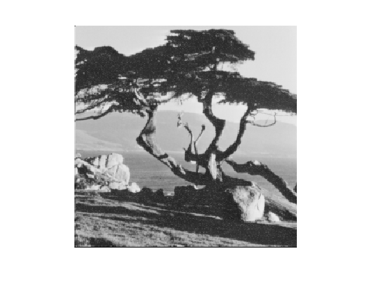
Figure 1: Set of test images: (a-b) natural images (c-d) texture images (e) aerial image (f) satellite image.
Refer to caption
(a) Noisy
Refer to caption
(b) SYS
Refer to caption
(c) ACPDE
Refer to caption
(d) Proposed
Figure 2: A 512×512512\times 512 brick image corrupted by Gaussian noise with σ=60\sigma=60 and restored by different models: (b) λ=0.8,K=5\lambda=0.8,K=5 (c) κ=1,ν=1,k=5\kappa=1,\nu=1,k=5 (d) α=2,β=20,k=4.5,ν=1.\alpha=2,\beta=20,k=4.5,\nu=1.
Refer to caption
(a)
Refer to caption
(b)
Refer to caption
(c)
Refer to caption
(d)
Refer to caption
(e)
Refer to caption
(f)
Refer to caption
(g)
Refer to caption
(h)
Figure 3: Restored signal by different models when the Brick image is corrupted by Gaussian noise with σ=20\sigma=20: (a) Original image showing the 1D slice (b) Clear signal (c) Noisy model (d) TDM; λ=5,K=15\lambda=5,K=15 (e)Cao; λ=20,K=6\lambda=20,K=6 (f) SYS; λ=2,K=5\lambda=2,K=5 (g) ACPDE; κ=1,ν=1,k=3\kappa=1,\nu=1,k=3 (h) Proposed; α=1,β=20,k=1.15,ν=1.\alpha=1,\beta=20,k=1.15,\nu=1.
Refer to caption
(a)
Refer to caption
(b)
Refer to caption
(c)
Refer to caption
(d)
Refer to caption
(e)
Refer to caption
(f)
Refer to caption
(g)
Refer to caption
(h)
Refer to caption
(i)
Refer to caption
(j)
Refer to caption
(k)
Refer to caption
(l)
Refer to caption
(m)
Refer to caption
(n)
Refer to caption
(o)
Figure 4: A 512×512512\times 512 mosaic image corrupted by Gaussian noise with σ=100\sigma=100 and restored by different models. (a) Original (b) Noisy (c) 3D surface plot of Noisy image (d-f) Cao; λ=20,K=6\lambda=20,K=6 (g-i) SYS; λ=0.1,K=5\lambda=0.1,K=5 (j-l) ACPDE; κ=1,ν=1,k=5\kappa=1,\nu=1,k=5 (m-o) Proposed; α=2,β=1,k=5,ν=1.\alpha=2,\beta=1,k=5,\nu=1.
Table 1: Comparison of MSSIM and PSNR values of denoised images using various approaches for images corrupted by a additive Gaussian noise with different noise level ( standard deviation:σ\sigma)
Image σ\sigma TDM[23] Cao [3] SYS[27] ACPDE[10] Proposed
MSSIM PSNR MSSIM PSNR MSSIM PSNR MSSIM PSNR MSSIM PSNR
Peppers 20 0.8865 29.64 0.8878 29.89 0.8826 29.85 0.9165 31.04 0.9375 31.33
40 0.8215 27.12 0.8273 27.27 0.8264 26.88 0.8506 27.80 0.8882 28.24
60 0.7655 25.30 0.7718 25.41 0.7397 24.96 0.7985 25.66 0.8344 26.02
80 0.7148 23.53 0.7225 23.61 0.6937 23.23 0.7520 23.73 0.7918 24.05
100 0.6523 21.84 0.6600 21.89 0.6255 21.63 0.6888 21.98 0.7357 22.23
Tree 20 0.7864 26.80 0.7802 27.24 0.7809 27.19 0.8360 27.99 0.8416 28.10
40 0.7500 24.26 0.7046 24.41 0.7065 23.98 0.7633 24.86 0.7689 24.99
60 0.6893 22.35 0.6490 22.42 0.6371 22.04 0.7058 22.68 0.7081 22.79
80 0.6287 20.63 0.5919 20.71 0.5674 20.36 0.6480 20.89 0.6495 21.01
100 0.5769 19.20 0.5451 19.29 0.5109 19.04 0.5974 19.43 0.5999 19.51
Mosaic 20 0.9516 33.64 0.9164 32.54 0.9258 32.59 0.9680 34.52 0.9884 34.53
40 0.9168 29.54 0.8666 28.81 0.8361 28.22 0.9436 29.79 0.9707 30.03
60 0.8838 26.06 0.8267 25.63 0.7838 25.08 0.9153 26.17 0.9324 26.26
80 0.8449 23.24 0.7818 22.98 0.6950 22.56 0.8839 23.33 0.9053 23.43
100 0.8096 21.08 0.7455 20.91 0.6889 20.62 0.8534 21.16 0.8784 21.23
Brick 20 0.8622 27.28 0.8634 27.37 0.8635 27.22 0.8610 27.31 0.8645 27.42
40 0.7335 24.66 0.7419 24.87 0.7391 24.66 0.7326 24.97 0.7433 25.00
60 0.6505 23.30 0.6578 23.44 0.6495 23.15 0.6638 23.64 0.6691 23.72
80 0.5839 22.08 0.5911 22.20 0.5768 21.88 0.5992 22.31 0.6039 22.35
100 0.5244 21.04 0.5306 21.12 0.5145 20.87 0.5347 21.15 0.5405 21.22
Aerial 20 0.8981 26.39 0.8969 26.38 0.8978 26.31 0.8999 26.48 0.9004 26.49
40 0.7789 23.85 0.7800 23.85 0.7766 23.76 0.7820 23.87 0.7840 23.90
60 0.6776 22.56 0.6827 22.56 0.6792 22.47 0.6857 22.57 0.6910 22.60
80 0.5893 21.56 0.5962 21.57 0.5912 21.48 0.5968 21.57 0.5973 21.57
100 0.5283 20.79 0.5367 20.79 0.5319 20.71 0.5372 20.79 0.5380 20.80
Moon 20 0.6763 29.58 0.6676 29.49 0.6790 29.69 0.6815 29.75 0.6817 29.80
40 0.5903 27.71 0.5860 27.56 0.5882 27.54 0.5960 27.90 0.5973 27.93
60 0.5606 26.71 0.5564 26.57 0.5519 26.38 0.5615 26.84 0.5663 26.97
80 0.5354 25.70 0.5318 25.59 0.5279 25.40 0.5357 25.83 0.5416 25.97
100 0.5206 24.69 0.5183 24.61 0.5160 24.49 0.5209 24.77 0.5241 24.89

5 Conclusion

A non-linear coupled telegraph diffusion equation based model for image denoising is introduced in this paper. Here we have taken telegraph equation for the image variable as well as for the edge variable, which improves the present model over the existing coupled PDE based models. Mathematical analysis of the model has been carried out using Banach’s fixed point theorem. Also, to validate the effectiveness of the proposed model, numerical experiments are carried out using different standard test images. Qualitative and quantitative studies, in terms of MSSIM, PSNR, and visual quality, confirm that the proposed model exhibits better performance than the single telegraph-diffusion based models as well as coupled partial differential equation models. This system not only removes the noise but also reduces the staircase artifacts and improves the performance of the filtering, even in low SNR images. Overall, the proposed model is an important addition in the field of diffusion equation based image restoration.

References

  • [1] G. Aubert, P. Kornprobst, Mathematical problems in image processing: partial differential equations and the calculus of variations, Vol. 147, Springer, 2006.
  • [2] Averbuch, A., Epstein, B., Rabin, N., Turkel, E.: Edge-enhancement postprocessing using artificial dissipation. IEEE transactions on image processing 15(6), 1486-1498 (2006)
  • [3] Cao, Y., Yin, J., Liu, Q., Li, M.: A class of nonlinear parabolic-hyperbolic equations applied to image restoration. Nonlinear Analysis: Real World Applications 11(1), 253-261 (2010)
  • [4] A. Chambolle, P.-L. Lions, Image recovery via total variation minimization and related problems, Numerische Mathematik 76 (2) (1997) 167-188.
  • [5] Deng, L., Zhu, H., Yang, Z., Li, Y.: Hessian matrix-based fourth-order anisotropic diffusion filter for image denoising. Optics &\& Laser Technology 110, 184-190 (2019)
  • [6] L. Evans, Partial Differential Equations, in: Graduate Studies in Mathematics, Vol. 19, American Mathematical Society, Providence, Rhode Island, 1998.
  • [7] R. C. Gonzalez, R. E. Woods, Digital image processing (2002).
  • [8] P. Guidotti, Anisotropic diffusions of image processing from perona-malik on, Advanced Studies in Pure Mathematics 99 (2015) 20XX.
  • [9] Z. Guo, J. Yin, Q. Liu, On a reaction-diffusion system applied to image decomposition and restoration, Mathematical and Computer Modelling 53 (5) (2011) 1336-1350.
  • [10] Jain, S.K., Majee, S., Ray, R.K., Majee, A.K.: Analysis and simulation of a coupled diffusion based image denoising model (2019), a preprint, arXiv arXivpreprintarXiv:1907.04526 (2019)
  • [11] Jain, S.K., Ray, R.K.: A non-linear diffusion based partial differential equation model for noise reduction in images. In: Information Systems Design and Intelligent Applications, pp. 429-438. Springer (2015)
  • [12] Jain, S.K., Ray, R.K.: An alternative framework of anisotropic diffusion for image denoising. In: Proceedings of the Second International Conference on Information and Communication Technology for Competitive Strategies, p. 46. ACM (2016)
  • [13] Jain, S.K., Ray, R.K.: Edge detectors based telegraph total variational model for image filtering. In: Information Systems Design and Intelligent Applications, pp. 119-126. Springer (2016)
  • [14] S. K. Jain, R. K. Ray, A. Bhavsar, A comparative study of iterative solvers for image denoising, in: Proceedings of the 3rd International Conference on Frontiers of Intelligent Computing: Theory and Applications (FICTA) 2014, Springer, 2015, pp. 307-314.
  • [15] S. K. Jain, R. K. Ray, A. Bhavsar,Iterative solvers for image denoising with diffusion models: A comparative study. Computers &\& Mathematics with Applications 70(3), 191-211 (2015)
  • [16] J. L. Lions, Contrôle Optimal de Systèmes Gouvernés par des Équations aux Dérivées Partielles, Dunod, Paris, 1968.
  • [17] Lions, J.L., Magenes, E.: Non-homogeneous boundary value problems and applications, vol. 2. Springer Science &\& Business Media (1972)
  • [18] X. Liu, L. Huang, Z. Guo, Adaptive fourth-order partial differential equation filter for image denoising, Applied Mathematics Letters 24 (8) (2011) 1282-1288.
  • [19] Liu, X., Lai, C.H., Pericleous, K.A.: A fourth-order partial differential equation denoising model with an adaptive relaxation method. International Journal of Computer Mathematics 92(3), 608-622 (2015)
  • [20] Lysaker, M., Lundervold, A., Tai, X.C.: Noise removal using fourth-order partial differential equation with applications to medical magnetic resonance images in space and time. IEEE Transactions on image processing 12(12), 1579-1590 (2003)
  • [21] M. Nitzberg, T. Shiota, Nonlinear image filtering with edge and corner enhancement, IEEE transactions on pattern analysis and machine intelligence 14 (8) (1992) 826-833.
  • [22] P. Perona, J. Malik, Scale-space and edge detection using anisotropic diffusion, Pattern Analysis and Machine Intelligence, IEEE Transactions on 12 (7) (1990) 629-639.
  • [23] Ratner, V., Zeevi, Y.Y.: Image enhancement using elastic manifolds. In: Image Analysis and Processing, 2007. ICIAP 2007. 14th International Conference on, pp. 769-774. IEEE (2007)
  • [24] L. I. Rudin, S. Osher, E. Fatemi, Nonlinear total variation based noise removal algorithms, Physica D: Nonlinear Phenomena 60 (1) (1992) 259-268.
  • [25] Scherzer, O.: Handbook of mathematical methods in imaging. Springer Science &\& Business Media (2010)
  • [26] A. Siddig, Z. Guo, Z. Zhou, B. Wu, An image denoising model based on a fourth-order nonlinear partial differential equation, Computers & Mathematics with Applications 76 (5) (2018) 1056-1074.
  • [27] J. Sun, J. Yang, L. Sun, A class of hyperbolic-parabolic coupled systems applied to image restoration, Boundary Value Problems 2016 (1) (2016) 187.
  • [28] Thanh, D.N., Prasath, V.S., Hieu, L.M.: A review on ct and x-ray images denoising methods. Informatica 43, 9pp (2019)
  • [29] Y.-H. R. Tsai, S. Osher, Total variation and level set methods in image science, Acta Numerica 14 (2005) 509-573.
  • [30] Wang, Z., Bovik, A.C.: Mean squared error: love it or leave it? a new look at signal fidelity measures. Signal Processing Magazine, IEEE 26(1), 98-117 (2009)
  • [31] J. Weickert, A review of nonlinear diffusion filtering, in: Scale-space theory in computer vision, Springer, 1997, pp. 1-28.
  • [32] J. Weickert, Anisotropic diffusion in image processing, Vol. 1, Teubner Stuttgart, 1998.
  • [33] Xu, J., Hao, Y., Li, M., Zhang, X.: A novel variational model for image decomposition. Signal, Image and Video Processing 13(5), 967-974 (2019)
  • [34] Yang, Y.Q., Zhang, C.Y.: Kernel based telegraph-diffusion equation for image noise removal. Mathematical Problems in Engineering 2014 (2014)
  • [35] You, Y.L., Kaveh, M.: Image enhancement using fourth order partial differential equations. In: Conference Record of Thirty- Second Asilomar Conference on Signals, Systems and Computers (Cat. No. 98CH36284), vol. 2, pp. 1677-1681. IEEE (1998)
  • [36] Y.-L. You, M. Kaveh, Fourth-order partial differential equations for noise removal, IEEE Transactions on Image Processing 9 (10) (2000) 1723-1730.
  • [37] R. Zanella, F. Porta, V. Ruggiero, M. Zanetti, Serial and parallel approaches for image segmentation by numerical minimization of a second-order functional, Applied Mathematics and Computation 318 (2018) 153-175.
  • [38] Zanetti, M., Ruggiero, V., Miranda Jr, M.: Numerical minimization of a second-order functional for image segmentation. Communications in nonlinear science and numerical simulation 36, 528-548 (2016)
  • [39] Zhang, X., Ye, W.: An adaptive fourth-order partial differential equation for image denoising. Computers &\& Mathematics with Applications 74(10), 2529-2545 (2017)
  • [40] S. Zheng, Nonlinear parabolic equations and hyperbolic-parabolic coupled systems, CRC Press, 1995.