Hamiltonian Dynamics of Semiclassical Gaussian Wave Packets in Electromagnetic Potentials

Gaussian wave packets have historically been used to solve the time-dependent semiclassical Schrödinger equation [7, 8, 9, 3, 6, 13]. While the Schrödinger equation is computationally non-trivial to solve in the semiclassical regime, those methods using the Gaussian wave packets provide an alternative set of differential equations that may be solved for the time-dependent parameters of the Gaussian wave packet. The Gaussian wave packet is an ansatz for an exact solution in the case of linear vector potentials with quadratic scalar potentials (see Hagedorn 1998), and gives a good short time approximation of the solution for other potentials in the semiclassical regime as shown by Zhou 2014.

However, the set of differential equations of Zhou for the parameters is not a Hamiltonian system in general. Given that the equations of motion for a classical particle is a Hamiltonian system and also that the Schrödinger equation is a (infinite-dimensional) Hamiltonian system as we will explain in a moment, it is rather natural to seek a Hamiltonian formulation of the dynamics of the Gaussian wave packet. This was the main motivation of our previous work [24] on the symplectic/Hamiltonian formulation of the Gaussian wave packet dynamics.

In this paper, we utilize the same symplectic-geometric framework to derive a Hamiltonian system of equations governing the evolution the wave packet parameters under the influence of electromagnetic fields by taking into account a vector potential. Semiclassical dynamics under the influence of electromagnetic fields has been of great interest recently because of its significance in quantum control and solid state physics.

It is well known that the equations of motion of a classical particle in $\mathbb{R}^{d}$ is a Hamiltonian system. From the symplectic-geometric point of view, one takes the cotangent bundle $T^{*}\mathbb{R}^{d}\cong\mathbb{R}^{2d}=\{(q,p)\,|\,q,p\in\mathbb{R}^{d}\}$ as the phase space and define the classical symplectic form $\Omega_{0}\mathrel{\mathop{:}}=\mathbf{d}q_{i}\wedge\mathbf{d}p_{i}$ (the Einstein summation convention is assumed). This renders $T^{*}\mathbb{R}^{d}$ a symplectic manifold. We also define a Hamiltonian function $H_{0}\colon T^{*}\mathbb{R}^{d}\to\mathbb{R}$ as

where $V\colon\mathbb{R}^{d}\rightarrow\mathbb{R}$ and $\boldsymbol{A}\colon\mathbb{R}^{d}\rightarrow\mathbb{R}^{d}$ are scalar and vector potentials respectively, and we set the charge to be 1 for simplicity.

Now let $X_{H_{0}}=\dot{q}_{i}\frac{\partial}{\partial q_{i}}+\dot{p}_{i}\frac{\partial}{\partial p_{i}}$ be the vector field on $T^{*}\mathbb{R}^{d}$ defined by $\textbf{i}_{X_{H_{0}}}\Omega_{0}=\textbf{d}H_{0}$ where $\mathbf{i}$ stands for the contraction. Then the equation yields the equations of motion of the classical particle in the electromagnetic field:

where $\gradient_{q}$ stands for the gradient with respect to the variable $q$, and $|\,\cdot\,|$ stands for the Euclidean distance in $\mathbb{R}^{d}$.

We may generalize the notion of Hamiltonian system as follows: Let $P$ be a symplectic manifold, i.e., a manifold equipped with a closed non-degenerate 2-form $\Omega$, and let $H\colon P\to\mathbb{R}$ be a smooth function. Then we define the Hamiltonian vector field $X_{H}$ on $P$ corresponding to the Hamiltonian function $H$ by setting $\textbf{i}_{X_{H}}\Omega=\textbf{d}H$. The vector field $X_{H}$ then defines the evolution equation on $P$. We may take it as the definition of a generalized Hamiltonian system; see, e.g., Marsden and Ratiu 1999 for more details.

We may now formulate the time-dependent Schrödinger equation as a Hamiltonian system as follows: Let $\mathcal{H}\mathrel{\mathop{:}}=L^{2}(\mathbb{R}^{d})$ with the standard (right-linear) inner product $\left\langle\,\cdot\,,\,\cdot\,\right\rangle$, and equip it with the symplectic form $\Omega_{\mathcal{H}}(\psi_{1},\psi_{2})\mathrel{\mathop{:}}=2\hbar\imaginary\left\langle\psi_{1},\psi_{2}\right\rangle$, and take the expectation value $\langle H\rangle\colon\mathcal{H}\to\mathbb{R}$ of the Hamiltonian operator as the Hamiltonian function. Then the Hamiltonian vector field $X_{\langle H\rangle}$ on $\mathcal{H}$ defined by $\textbf{i}_{X_{\langle H\rangle}}\Omega_{\mathcal{H}}=\textbf{d}\langle H\rangle$ yields the usual time-dependent Schrödinger equation

where $\hat{H}$ is the Hamiltonian operator defined below.

Given that the basic equations of classical and quantum dynamics are both Hamiltonian systems, it is natural to expect that the basic equations of semiclassical dynamics—or more generally approximation/reduced models of quantum dynamics—are Hamiltonian as well. Is there a way to exploit the above symplectic structure $\Omega_{\mathcal{H}}$ on $\mathcal{H}=L^{2}(\mathbb{R}^{d})$ to find a Hamiltonian formulation of reduced models?

Lubich 2008 (see also Kramer and Saraceno 1981) came up with a general prescription to achieve this by geometrically interpreting approximation models of quantum dynamics. Suppose that we have an ansatz $\varphi\colon M\to\mathcal{H}\mathrel{\mathop{:}}=L^{2}(\mathbb{R}^{d});y\mapsto\varphi(y;\,\cdot\,)$ for the solution of the Schrödinger equation, where $M$ is a finite-dimensional manifold (where the parameters for the ansatz live). The parameters $y$ evolve in time according to the dynamics in $M$ to be determined, and the time evolution $t\mapsto\varphi(y(t);\,\cdot\,)$ gives an approximation to the solution of the Schrödinger equation (3). Lubich 2008 (see also Ohsawa and Leok 2013) showed that one can achieve the best approximation in $M$ as follows: Consider the embedding $\iota\colon M\rightarrow\mathcal{H}$ defined by the ansatz $\varphi$ as $\iota(y)\mathrel{\mathop{:}}=\varphi(y;\,\cdot\,)$. Then we can pull back the symplectic form $\Omega_{\mathcal{H}}$ to $M$ to obtain a 2-form $\Omega\mathrel{\mathop{:}}=\iota^{*}\Omega_{\mathcal{H}}$ on $M$. Under a certain technical condition (see [14] and [24, Proposition 2.1] for details), $\Omega$ defines a symplectic form on $M$. One may also define the pull-back $H\mathrel{\mathop{:}}=\langle H\rangle\circ\iota$ of the Hamiltonian function, i.e., $H(y)\mathrel{\mathop{:}}=\left\langle\varphi(y;\,\cdot\,),\hat{H}\varphi(y;\,\cdot\,)\right\rangle$. Then we may define the Hamiltonian vector field $X_{H}$ on $M$ by setting $\textbf{i}_{X_{H}}\Omega=\textbf{d}H$. Lubich 2008 showed that this gives the least squares approximation of the vector field $X_{\langle H\rangle}$ in the following sense: For any $y\in M$ and any $V_{y}\in T_{y}M$,

in terms of the $L^{2}$ norm in $\mathcal{H}=L^{2}(\mathbb{R}^{d})$; see Fig. 1.

Our ansatz or approximation/reduced model is the Gaussian wave packet of Heller 1975, Heller 1976, Heller 1981 and Hagedorn 1980, Hagedorn 1998 (see also Littlejohn 1986):

where $(q,p)\in T^{*}\mathbb{R}^{d}\cong\mathbb{R}^{2d}$ is the phase space center, $\phi$ $\in$ $\mathbb{S}^{1}$ is the phase factor, $\delta$ $\in$ $\mathbb{R}$ controls the norm, and $\mathcal{A}+\text{i}\mathcal{B}\in\Sigma_{d}\mathrel{\mathop{:}}=\{\mathcal{A}+\text{i}\mathcal{B}\in\mathbb{C}^{d\times d}\,|\,\mathcal{A},\mathcal{B}\in\text{Sym}_{d}(\mathbb{R}),\mathcal{B}-\text{positive definite}\}$. Note that the above Gaussian is not normalized:

where we set $y=({q},{p},\mathcal{A},\mathcal{B},\phi,\delta)$. We will address this issue later.

Following the geometric picture of Lubich 2008 described above, we define $M$ to be the space of the above parameters:

and consider the embedding $\iota\colon M\to\mathcal{H}$ defined as $\iota(y)\mathrel{\mathop{:}}=\chi_{M}(y;\,\cdot\,)$. Then one can show that the pull-back $\Omega_{M}\mathrel{\mathop{:}}=\iota^{*}\Omega_{\mathcal{H}}$ is in fact a symplectic form on $M$; see Ohsawa and Leok 2013.

In this paper, we would like to incorporate the effect of electromagnetic fields to the dynamics of the Gaussian wave packet. So we take Hamiltonian operator $\hat{H}$ to be

where we assume that the scalar and vector potentials $V\colon\mathbb{R}^{d}\rightarrow\mathbb{R}$ and $\boldsymbol{A}\colon\mathbb{R}^{d}\rightarrow\mathbb{R}^{d}$ are smooth functions; we write the $i$-th component of $\boldsymbol{A}_{i}$ as opposed to the more conventional $A_{i}$ in order to make it more conspicuous and to avoid possible confusions with the components of $\mathcal{A}$.

One may then evaluate the pull-back $H_{M}\mathrel{\mathop{:}}=\langle H\rangle\circ\iota\colon M\to\mathbb{R}$ of the Hamiltonian $\langle H\rangle$ by evaluating the expectation value of the Hamiltonian operator as follows:

where $\boldsymbol{A}$ is regarded as a column vector, $D\boldsymbol{A}(x)$ is the $d\times d$ matrix whose $(i,j)$-component is $\frac{\partial\boldsymbol{A}_{i}}{\partial x_{j}}(x)$, and $\langle\,\cdot\,\rangle$ stands for the expectation value of an observable with respect to the normalized Gaussian $\chi_{M}/\norm{\chi_{M}}$: For any smooth function $\mathcal{U}\colon\mathbb{R}^{d}\to\mathbb{R}$ satisfying a certain growth condition (see Section 3.1),

One may now certainly formulate a Hamiltonian system on $M$ using the above pull-backs of the symplectic form and the Hamiltonian. However, the pull-back of the symplectic form turns out to be very cumbersome; neither does it provide much insight into its relationship with the symplectic form $\Omega_{0}$ of classical dynamics; see Ohsawa and Leok 2013.

Fortunately, there is a way around it to obtain a simpler and more appealing formulation by exploiting the inherent symmetry of the system [24, Section 4]. First observe that the Hamiltonian (6) does not depend on the phase factor variable $\phi$; that is, the Hamiltonian is invariant under the following $\mathbb{S}^{1}$-action on the manifold $M$:

This action turns out to be symplectic and the corresponding momentum map (Noether conserved quantity) is

It is natural to look at the level set $\mathbf{N}^{-1}(-\hbar)$ because, in view of the definition (5) of $\mathcal{N}$, this level set corresponds to the choice of the parameter $\delta$ so that the Gaussian $\chi_{M}$ is normalized, i.e., $\norm{\chi(y;\,\cdot\,)}=1$. Furthermore, one may eliminate the variables $(\phi,\delta)$ from the formulation, because now we may apply the Marsden–Weinstein reduction [16] (see also Marsden et al. 2007) to obtain the reduced symplectic manifold

See [24, Section 4] for the details of this reduction.

As a result, the symplectic form $\Omega_{M}$ on $M$ gives rise to the following symplectic form $\Omega_{\hbar}$ on $\overline{M}$:

Notice that the symplectic form is very simple and also appealing because it has an additional $\mathcal{O}(\hbar)$ correction term compared to the classical symplectic form $\Omega_{0}$. It is also clear from the above expressions that $\mathcal{B}^{-1}$ and $\mathcal{A}$ are conjugate variables. The corresponding Poisson Bracket is then

Since we are now looking at the normalized Gaussian, we have $\mathcal{N}(\mathcal{B},\delta)=1$, and thus the reduced Hamiltonian $H\colon\overline{M}\to\mathbb{R}$ becomes

The Hamiltonian vector field $X_{H}$ on $\overline{M}$ defined by the Hamiltonian system $\textbf{i}_{X_{H}}\Omega_{\hbar}=\textbf{d}H$ or equivalently $\dot{\bar{y}}=\left\{\bar{y},H\right\}_{\hbar}$ with $\bar{y}=(q,p,\mathcal{A},\mathcal{B})$ gives the following set of ordinary differential equations:

where $(D\boldsymbol{A})_{ij}=D_{j}\boldsymbol{A}_{i}=\frac{\partial\boldsymbol{A}_{i}}{\partial x_{j}}$, and $D^{2}_{ij}\boldsymbol{A}_{k}=\frac{\partial\boldsymbol{A}_{k}}{\partial x_{i}\partial x_{j}}$.

While the above set (10) of equations is Hamiltonian by construction, it has the drawback that it is not in a closed form: The potential terms—involving either the scalar potential $V$ or the vector potential $\boldsymbol{A}$—appear as expectation values (with respect to the normalized Gaussian). Unfortunately, it is impossible to explicitly evaluate these expectation values unless $V$ and $\boldsymbol{A}$ are polynomials.

So we apply Laplace’s method to obtain an asymptotic expansions of the integrals as $\hbar\to 0$ (see, e.g., Miller 2006). Assuming that the Gaussian is normalized, i.e., $\mathcal{N}(\mathcal{B},\delta)=1$, each potential term is of the form (see (7)):

As is proved in Ohsawa and Leok 2013 (see also Miller 2006), if $\mathcal{U}$ satisfies a certain growth condition as $|x|\to\infty$, then $\left\langle\mathcal{U}\right\rangle$ has the following asymptotic expansion:

where $D^{2}\mathcal{U}(q)$ is the Hessian matrix of $\mathcal{U}(x)$ evaluated at $x=q$. We note in passing that this asymptotic expansion is exact (i.e., the $O(\hbar^{2})$ term vanishes) if $\mathcal{U}$ is quadratic.

As a result, we have the following asymptotic expansion for the Hamiltonian $H$ from (6):

with

Notice that, just as for the symplectic form $\Omega$ in (8), this semiclassical Hamiltonian $H$ has an additional $\mathcal{O}(\hbar)$ correction term compared to the classical Hamiltonian $H_{0}$ from (1).

One may now replace the Hamiltonian $H$ by $H_{\hbar}$ to define the Hamiltonian vector field $X_{H_{\hbar}}$ as $\textbf{i}_{X_{H_{\hbar}}}\Omega_{\hbar}=\textbf{d}H_{\hbar}$. Then the vector field $X_{H_{\hbar}}$ yields

If we define those terms involving scalar and vector potentials with $O(\hbar)$ corrections as

we can rewrite the first two of the above set of equations in a slightly more succinct form:

Notice also its similarity to the classical equations (2).

As mentioned in the Introduction, when the vector potential $\boldsymbol{A}$ is linear ($\boldsymbol{A}(x)=Ax$, where $A$ is a constant $d\times d$ matrix) and the scalar potential $V$ is quadratic, the Gaussian wave packet (4) gives an exact solution to the Schrödinger equation if the parameters satisfy the following set of equations (along with additional equations for $\phi$ and $\delta$):

This result is a special case of the more general result of Hagedorn 1998 on quadratic Hamiltonians, and also is equivalent to the set of equations given by Zhou 2014. We note that both Hagedorn 1998 and Zhou 2014 use, instead of $(\mathcal{A},\mathcal{B})$, parameters $(Q,P)$ that are $d\times d$ complex matrices satisfying $Q^{T}P-P^{T}Q=0$ and $Q^{*}P-P^{*}Q=2\text{i}I_{d}$; more precisely, Hagedorn 1998 uses parameters $A,B\in\mathbb{C}^{d\times d}$, which are related to $Q$ and $P$ as $A=Q$ and $B=-\text{i}P$. In fact, these two sets of parameters are related by $\mathcal{A}+\text{i}\mathcal{B}=PQ^{-1}$; see Ohsawa 2015b for the geometric interpretation of these two different parametrizations. It is straightforward calculations using this relation to check that Zhou 2014’s equations imply the above set of equations.

Our set of equations, either (10) or (13), recovers the above set of equations under the above assumptions on the potentials. In fact, as mentioned above, the asymptotic expansion (11) is exact if $\mathcal{U}$ is quadratic. This implies that the Hamiltonian (9) and its $\mathcal{O}(\hbar^{2})$ approximation (12) coincide, and thus so do the equations (10) and (13). Now, if the vector potential $\boldsymbol{A}$ is linear and the scalar potential $V$ is quadratic, many of the terms in (13) involving the Hessians of the potentials vanish, hence recovering (14).

Suppose that the scalar and vector potentials $V$ and $\boldsymbol{A}$ possess the rotational symmetry in the following sense: For any $R\in\mathsf{SO}(d)$ and any $x\in\mathbb{R}^{d}$,

that is, $V$ is $\mathsf{SO}(d)$-invariant whereas $\boldsymbol{A}$ is $\mathsf{SO}(d)$-equivariant. We note that the latter condition implies $D\boldsymbol{A}(Rx)=R\boldsymbol{A}(x)R^{T}$ for any $R\in\mathsf{SO}(d)$ and any $x\in\mathbb{R}^{d}$.

As is done in [22], we define the action of the rotation group $\mathsf{SO}(d)$ on the symplectic manifold $\overline{M}=T^{*}\mathbb{R}^{d}\times\Sigma_{d}$ as follows:

It is easy to check that $\Gamma$ is symplectic, i.e., $\Gamma^{*}_{R}\Omega=\Omega$ for any $R\in\mathsf{SO}(d)$. Then our Hamiltonian, either (9) or (12), is invariant under this action, i.e., for any $R\in\mathsf{SO}(d)$, $H\circ\Gamma_{R}=H$ and $H_{\hbar}\circ\Gamma_{R}=H_{\hbar}$. In fact, for the Hamiltonian (12), it follows from a straightforward calculation using the above symmetry assumptions on $V$ and $\boldsymbol{A}$. For the Hamiltonian (9), note that the expectation values of the potentials maintain the same symmetry, i.e.,

The momentum map $\mathbf{J}_{\hbar}\colon\overline{M}\to\mathfrak{so}(d)^{*}$ corresponding to the action $\Gamma$ defined above is given by (see Ohsawa 2015a for the derivation)

where $(q\diamond p)_{ij}=q_{j}p_{i}-q_{i}p_{j}$ (see Holm 2011), and we identified $\mathfrak{so}(d)^{*}$ with $\mathfrak{so}(d)$ via an inner product. Setting $\hbar=0$ reduces the above to the classical angular momentum, hence we call the above the semiclassical angular momentum. Interestingly, this semiclassical angular momentum coincides with the expectation value of the angular momentum with respect to the normalized Gaussian, i.e., for $d=3$,

Now, assuming the symmetry (15) in the potentials, by Noether’s Theorem (see, e.g., Marsden and Ratiu 1999), we conclude that the semiclassical angular momentum (16) is a conserved quantity of our semiclassical equation (10) or (13).

Here we let $d=1$, $m=1$, $V(x)=1-\frac{1}{2}\cos^{2}(x)$, $A(x)=\cos(x)$, subject to the initial conditions $q(0)=0.5$, $p(0)=-1$, $\mathcal{A}(0)=0$, $\mathcal{B}(0)=1$; the scalar and vector potentials are taken from Zhou 2014. In order to see how the error converges as $\hbar\to 0$, we ran the computations for $\hbar=0.5,0.3,0.1,0.05,0.03,0.01$.

Figure 2 shows the solutions on the classical phase space $T^{*}\mathbb{R}=\mathbb{R}^{2}$ from $t=0$ to $t=3$ as well as the error $|\langle\hat{z}\rangle(t)-z(t)|$ at $t=1.6$ in terms of the Euclidean norm on the classical phase space. As can be seen, our solutions are closer to the Egorov/IVR than the classical solutions. Furthermore, as $\hbar\rightarrow 0$, our solutions converge to the Egorov/IVR solutions faster than the classical equations.

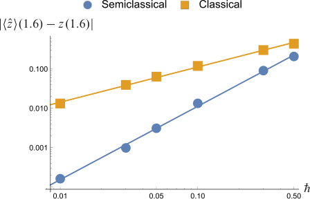
Figure 3 shows the time evolutions of the Hamiltonians for the classical, semiclassical, and Egorov/IVR solutions. Note that the Hamiltonians for all these three cases are different: It is $H_{0}$ in (1) for the classical case and $H_{\hbar}$ in (12) for the semiclassical case, whereas for the Egorov/IVR case, it is the expectation value $\langle\hat{H}\rangle$ of the Hamiltonian operator $\hat{H}$. In each of these cases, the corresponding Hamiltonian is a conserved quantity. Notice that the semiclassical Hamiltonian gives a better approximation to the expectation value of the Hamiltonian.

Here we let $d=2$, $V(x)=\frac{1}{2}|x|^{2}+\frac{1}{4}|x|^{4}$, $A(x)=(-x_{2},x_{1})$, subject to the initial conditions $q(0)=(1,0)$, $p(0)=(0,1)$, $\mathcal{A}(0)=\begin{pmatrix}-3&-6\\ -6&-6\end{pmatrix}$, $\mathcal{B}(0)=\begin{pmatrix}1&1/2\\ 1/2&1\end{pmatrix}$.

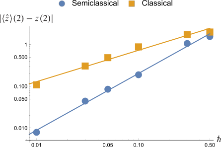
Figure 4 shows the solutions on the classical configuration space $\mathbb{R}^{2}=\{(q_{1},q_{2})\}$ from $t=0$ to $t=10$ as well as the error $|\langle\hat{z}\rangle(t)-z(t)|$ at $t=2$ in terms of the Euclidean norm on the classical phase space $T^{*}\mathbb{R}^{2}\cong\mathbb{R}^{4}$. Figure 5 shows the time evolutions of the Hamiltonians for the classical, semiclassical, and Egorov/IVR solutions just as in the 1D case. The same observations as above apply to these 2D results as well.

For this 2D example, the scalar and vector potentials chosen above satisfy the symmetry condition (15). Therefore, based on the result of Section 4, the semiclassical angular momentum (16) is also a conserved quantity of the semiclassical system (13) as well. Figure 6 shows the time evolutions of the classical angular momentum along the classical solutions, the semiclassical angular momentum (16) along the semiclassical solutions, and the expectation value of the angular momentum operator along the Egorov/IVR solutions. We see that the semiclassical angular momentum gives a better approximation to the expectation value of the angular momentum than the classical one does.

References

- Combescure and Robert [2012] M. Combescure and D. Robert. Coherent States and Applications in Mathematical Physics. Springer, 2012.
- Egorov [1969] Y. V. Egorov. The canonical transformations of pseudodifferential operators. Uspekhi Mat. Nauk, 24(5(149)):235–236, 1969.
- Hagedorn [1980] G. A. Hagedorn. Semiclassical quantum mechanics. I. The limit for coherent states. Communications in Mathematical Physics, 71(1):77–93, 1980.
- Hagedorn [1981] G. A. Hagedorn. Semiclassical quantum mechanics. III. the large order asymptotics and more general states. Annals of Physics, 135(1):58–70, 1981.
- Hagedorn [1985] G. A. Hagedorn. Semiclassical quantum mechanics, IV: large order asymptotics and more general states in more than one dimension. Annales de l’institut Henri Poincaré (A) Physique théorique, 42(4):363–374, 1985.
- Hagedorn [1998] G. A. Hagedorn. Raising and lowering operators for semiclassical wave packets. Annals of Physics, 269(1):77–104, 1998.
- Heller [1975] E. J. Heller. Time-dependent approach to semiclassical dynamics. Journal of Chemical Physics, 62(4):1544–1555, 1975.
- Heller [1976] E. J. Heller. Classical -matrix limit of wave packet dynamics. Journal of Chemical Physics, 65(11):4979–4989, 1976.
- Heller [1981] E. J. Heller. Frozen Gaussians: A very simple semiclassical approximation. Journal of Chemical Physics, 75(6):2923–2931, 1981.
- Holm [2011] D. D. Holm. Geometric Mechanics, Part II: Rotating, Translating and Rolling. Imperial College Press, 2nd edition, 2011.
- Kramer and Saraceno [1981] P. Kramer and M. Saraceno. Geometry of the time-dependent variational principle in quantum mechanics. Lecture notes in physics. Springer-Verlag, 1981.
- Lasser and Röblitz [2010] C. Lasser and S. Röblitz. Computing expectation values for molecular quantum dynamics. SIAM Journal on Scientific Computing, 32(3):1465–1483, 2010.
- Littlejohn [1986] R. G. Littlejohn. The semiclassical evolution of wave packets. Physics Reports, 138(4-5):193–291, 1986.
- Lubich [2008] C. Lubich. From quantum to classical molecular dynamics: reduced models and numerical analysis. European Mathematical Society, Zürich, Switzerland, 2008.
- Marsden and Ratiu [1999] J. E. Marsden and T. S. Ratiu. Introduction to Mechanics and Symmetry. Springer, 1999.
- Marsden and Weinstein [1974] J. E. Marsden and A. Weinstein. Reduction of symplectic manifolds with symmetry. Reports on Mathematical Physics, 5(1):121–130, 1974.
- Marsden et al. [2007] J. E. Marsden, G. Misiolek, J. P. Ortega, M. Perlmutter, and T. S. Ratiu. Hamiltonian Reduction by Stages. Springer, 2007.
- Miller [2006] P. D. Miller. Applied Asymptotic Analysis. American Mathematical Society, Providence, R.I., 2006.
- Miller [1970] W. H. Miller. Classical S matrix: Numerical application to inelastic collisions. The Journal of Chemical Physics, 53(9):3578–3587, 1970.
- Miller [1974] W. H. Miller. Quantum mechanical transition state theory and a new semiclassical model for reaction rate constants. The Journal of Chemical Physics, 61(5):1823–1834, 1974.
- Miller [2001] W. H. Miller. The semiclassical initial value representation: A potentially practical way for adding quantum effects to classical molecular dynamics simulations. The Journal of Physical Chemistry A, 105(13):2942–2955, 2001.
- Ohsawa [2015a] T. Ohsawa. Symmetry and conservation laws in semiclassical wave packet dynamics. Journal of Mathematical Physics, 56(3):032103, 2015a.
- Ohsawa [2015b] T. Ohsawa. The Siegel upper half space is a Marsden–Weinstein quotient: Symplectic reduction and Gaussian wave packets. Letters in Mathematical Physics, 105(9):1301–1320, 2015b.
- Ohsawa and Leok [2013] T. Ohsawa and M. Leok. Symplectic semiclassical wave packet dynamics. Journal of Physics A: Mathematical and Theoretical, 46(40):405201, 2013.
- Wang et al. [1998] H. Wang, X. Sun, and W. H. Miller. Semiclassical approximations for the calculation of thermal rate constants for chemical reactions in complex molecular systems. The Journal of Chemical Physics, 108(23):9726–9736, 1998.
- Zhou [2014] Z. Zhou. Numerical approximation of the Schrödinger equation with the electromagnetic field by the Hagedorn wave packets. Journal of Computational Physics, 272:386–407, 2014.