UMD-PP-019-04
Cosmological Collider Physics and the Curvaton
Abstract
Primordial non-Gaussianity signatures of extremely heavy particles are re-examined within a simple alternative to the standard inflationary paradigm, in which the primordial fluctuations and the inflationary spacetime expansion are sourced by two different fields. The curvaton scenario provides an example of this in which the distinct roles are played by the curvaton and the inflaton fields, respectively. We study couplings of the curvaton to heavy particles with masses of order the inflationary Hubble scale, and show that they can lead to non-Gaussian signals orders of magnitude larger than those in standard inflation, consistent with explicit effective field theory control of inflationary dynamics. This brings various motivated particle physics signatures, such as loops of heavy gauge-charged scalars and fermions, within future observational reach.
1 Introduction
An era of cosmic inflation (see Baumann:2009ds for a review) in the very early universe is an attractive paradigm to explain the origin and the properties of the primordial density perturbations that eventually seed the temperature fluctuations in cosmic microwave background (CMB) and the inhomogeneities in large scale structure (LSS). The simplest models of cosmic inflation predict that the primordial fluctuations are adiabatic, scale invariant and approximately Gaussian—all three of these properties are verified to a good extent by the observations Akrami:2018odb. Importantly, such properties can be tested with even better precision with upcoming surveys and this would allow us to get a more detailed picture of the inflationary era. In particular, any detection of primordial non-Gaussianity (NG) can give us crucial insight into physics at the inflationary Hubble scale , which could lie well beyond the reach of terrestrial experiments. The time dependent inflationary spacetime can produce new particles with masses . If such particles can decay into inflatons, they can give rise to a distinctive non-analytic momentum dependence and angular dependence of the three (and higher)-point correlation function of the primordial fluctuations. Through a careful measurement of such dependencies, one can infer the mass and spin of such heavy particles—a rare opportunity to probe on-shell physics at very high energy scales. This is the focus of the “cosmological collider physics” program Chen:2009zp; Baumann:2011nk; Assassi:2012zq; Chen:2012ge; Noumi:2012vr; Pi:2012gf; Gong:2013sma; Arkani-Hamed:2015bza; Lee:2016vti; Chen:2016nrs; Chen:2016uwp; Chen:2016hrz; Chen:2017ryl; Kehagias:2017cym; An:2017hlx; Kumar:2017ecc; Baumann:2017jvh. For various recent ideas in this direction see, Chen:2018xck; An:2018tcq; Chen:2018cgg; Kumar:2018jxz; Arkani-Hamed:2018kmz; Li:2019ves; Wu:2019ohx; Alexander:2019vtb; Lu:2019tjj; Hook:2019zxa; Hook:2019vcn.
To understand the prospects of detection of such heavy particle-induced NG, we can characterize the strength of NG by a dimensionless parameter, conventionally called in the literature, whose definition will be given in sec. 2. Current CMB constraints on varies depending on the particular shape of NG under consideration and broadly, is given by Akrami:2019izv. Upcoming LSS experiments will improve this by having a precision Alvarez:2014vva which will be useful to probe heavy particle-induced NG MoradinezhadDizgah:2017szk; MoradinezhadDizgah:2018ssw. The ultimate sensitivity in this regard will be provided by an only cosmic-variance-limited 21-cm experiment which can roughly achieve Meerburg:2016zdz. Thus we will consider as the ultimate limiting strength of NG for observability. Given this lower bound, with some rare exceptions Chen:2009zp, many of the prime targets of the cosmological collider program such as, massive gauge bosons Chen:2016hrz; Chen:2016nrs; Chen:2016uwp; Kumar:2017ecc; Kumar:2018jxz, charged scalars and fermions Chen:2016hrz; Chen:2016nrs; Chen:2016uwp; Kumar:2017ecc; Chen:2018xck; Hook:2019vcn; Hook:2019zxa, Kaluza-Klein modes of the graviton Kumar:2018jxz give rise to small, and sometimes even unobservable, strength of NG in the standard inflationary paradigm where the dynamics of inflation is explicitly described in terms of scalar fields. The primary goal of the present work is to describe a simple, alternative paradigm, in which the above mentioned NGs are naturally orders of magnitude larger, and the associated targets can naturally be brought into the scope of the cosmological collider program. Let us first understand what suppresses such NG contributions in the standard paradigm.
The inflaton () is a light field (with mass ) during inflation. To ensure that it remains light in the presence of potentially large radiative corrections due to heavy states, one normally imposes a shift symmetry , with being a constant, which is broken only weakly by its potential. Under the restriction of such a shift symmetry, the dominant coupling of to a generic operator is schematically described within an effective field theory (EFT) framework as,
| (1) |
where is the scaling dimension of the operator , and is a scale by which the EFT description must break down. Strengths of such non-renormalizable couplings are thus characterized by inverse powers of , and a smaller value of implies a larger coupling, leading to a larger strength of NG. So from an observational perspective, it is important to ask how small can be while our description still remains in theoretical control. Several possible choices of exist, with varying levels of conservatism and assumptions about the ultra-violet (UV) physics. A schematic representation of the relevant scales is shown in fig. 1.

Due to quantum gravity effects any EFT description is expected to break down at and thus can be a reasonable choice, assuming no new physics comes in between and . With such a high value of , the strength of NG is small, but can be observable in a few cases Chen:2009zp; Arkani-Hamed:2015bza; Kumar:2018jxz. Stronger NG can be obtained by taking where is the potential energy density that drives the inflationary expansion. Such a choice of is still conservative because is the highest energy scale available during and after inflation. For example the reheat temperature, , during the reheating stage at the end of inflation can be maximally . Thus an EFT with is capable of describing the universe both during and after inflation. Keeping this in mind, in this work we will take
| (2) |
where we have used the Planck constraint Akrami:2018odb on tensor-to-scalar ratio. We will show later that the above restriction (2) implies that the NG mediated by heavy particles in several scenarios of interest are quite small or even unobservable.
We note that if one only demands theoretical control of the series of higher dimensional terms in the EFT which involve an expansion in , a weaker restriction of can be obtained Creminelli:2003iq, where denotes the homogeneous part of the inflaton field and we have used the fact that the scalar power spectrum implies Akrami:2018odb. However, such low does not explicitly capture the scalar field source of inflation, . We will not pursue this less conservative here.
Even more agnostically, the Goldstone effective theory of inflation Cheung:2007st, which describes only the cosmological fluctuations during inflation, but not the dynamics driving inflation, can avoid even the restriction . To ensure control over the description of just the fluctuations which probe energy scales , one need only have the EFT cut off . One can then have stronger couplings between the inflationary fluctuations and -mass particles, leading to significantly larger NG than what is obtained by demanding (2).
This Goldstone description is completely agnostic about whether such low values of are consistent with higher scales such as and since the latter scales, which control the homogeneous background, do not even appear in the Goldstone dynamics of inflationary fluctuations. The Goldstone description simply assumes that a suitable homogeneous inflationary background is given. There do exist subtle mechanisms beyond the Goldstone description (e.g. Alishahiha:2004eh; Baumann:2011su) which achieve compatibility between the two sets of scales. In this work we explore a very simple alternative where such a compatibility is readily obtained. This is achieved by having an explicit separation of the field degrees of freedom responsible for the inflationary background and for seeding the density fluctuations. We assume that along with the inflaton field, there exists a second light field , the “curvaton” Enqvist:2001zp; Lyth:2001nq; Moroi:2001ct, whose role is to predominantly give rise to primordial fluctuations (today), whereas the role of the inflaton is reduced to just sourcing the background expansion (with subdominant fluctuations). Then it is completely consistent to have separate EFT cutoff scales for and , which automatically implies separate cutoffs for inflationary fluctuations and the homogeneous background. This can then naturally, but in a controlled way, lead to large NG if the EFT scale characterizing nonrenormalizable interactions is parametrically smaller than the EFT cutoff of dynamics.
Concretely, one can have and belong to two different sectors which are sequestered from each other (say, via having different locations in an extra dimension) with each having their own EFT cutoffs, and respectively. Since does not have to drive the background expansion, its energy density can be . Then an argument similar to the one leading to (2), will only imply
| (3) |
while still allowing . Such a scenario with can arise in several ways. One possibility is that the scale could represent the masses of new mediator fields which couple to and -mass particles, but not to . An example along this line will be studied in sec. 5. Another possibility is that could represent a compositeness/confinement scale for the sector and/or heavy fields interacting with it. Via the AdS/CFT duality, this latter scenario is dual to an extra-dimensional set-up where and are localized on two distinct “branes” and the extra-dimensional warping (redshifts) between the two branes explains why .
Since the two sectors are decoupled (up to gravitational effects) and can undergo separate reheating, does not lead to a break down of the EFT description for at the end of inflation. If the mass particles now couple to , such couplings need only be suppressed by , instead of , and thus one can then have orders of magnitude bigger NG of primordial density fluctuations. Compared to the Goldstone EFT of inflation framework, this scenario can successfully describe inflationary and post-inflationary dynamics as will be discussed in sec. 3, giving us an example of a controlled field theoretic scenario having potentially larger NG than the standard paradigm.
This paper is organized as follows. In sec. 2, we will set up the notation and discuss some essential aspects of the cosmological collider physics program. We will review the curvaton scenario and note the current set of observational constraints on it in sec. 3. The detailed analysis of the EFT couplings of the heavy particles will then be carried out, both in the standard inflationary scenario, sec. 4, and in the curvaton scenario, sec. 5. Three types of NG contribution of heavy particles—tree-level effects of spontaneously broken charged scalars (Higgs bosons), and loop-level effects of unbroken charged scalars and charged Dirac fermions will be considered. We will discuss an issue of classical tuning that arises in the inflationary paradigm and see that if we forego such tuning, the loop-mediated NG are unobservably small. While enhanced NG signals can be obtained with tuning, we will show that such tunings and enhancements are limited. The curvaton scenario will, on the other hand, have no such tunings but still gives rise to orders of magnitude larger NG compared to the standard inflationary scenario. In appendices A and B we will calculate the NG contributions explicitly to confirm those statements. We conclude in sec. 6. Throughout this paper we work in the sign convention for the spacetime metric.
As this paper was being completed, ref. Lu:2019tjj appeared which discusses how Higgs fluctuations, different from inflaton fluctuations, can source primordial density perturbations through reheating via Higgs-modulated inflaton decay. The curvaton scenario we present here allows a larger enhancement of NG signals compared to ref. Lu:2019tjj and also makes the robust prediction of the strength of a “local” type of NG, , absent in ref. Lu:2019tjj. Nevertheless, there are some structural similarities between the present work and ref. Lu:2019tjj.
2 Observables and cosmological collider physics
We denote the gauge invariant curvature perturbation, which will be defined below, by , and use the primed notation to denote its momentum space correlation functions,
| (4) |
The power spectrum is denoted by,
| (5) |
The dimensionless three point function parametrizing the strength of NG is defined as,
| (6) |
The function defined above is in general momentum dependent and thus it is conventional in the literature to define an “amplitude” of NG in the equilateral limit ,
| (7) |
Using the above definition of one has a very rough estimate of the precision by which can be measured in an only-cosmic-variance limited 21-cm experiment. Such a precision is controlled only by the number of modes and is given by,
| (8) |
Thus using the estimate Loeb:2003ya, one has very roughly .
We will be interested in the so-called “squeezed limit” of in eq. (6) for which . In that case, becomes a function of only . In particular, heavy fields with , can mediate non-analytic momentum dependence of of the type,
| (9) |
where . The functions depend on the mass and spin of the heavy particle and can be calculated given its coupling to the inflaton. The prospect of extracting the mass and spin of the such heavy fields via measuring and , forms the basis of cosmological collider physics. In the following, we will quantify the strength of NG by the absolute value .
While the time dependent inflationary spacetime readily produces particles with masses , production of heavier particles are “Boltzmann suppressed” with for . Furthermore, for , becomes analytically dependent on so that the distinctive non-analytic, on-shell information characterizing heavy-particle mediation is no longer apparent. For example, for a scalar particle, for . Thus the cosmological collider program operates most efficiently in a window of heavy masses around to give us on-shell mass and spin information.
3 Curvaton paradigm
3.1 Cosmological history
We will now briefly review the cosmological history in the curvaton paradigm and emphasize some of the important differences between it and the standard inflationary paradigm. For more details on the curvaton paradigm, the reader is referred to the original papers Enqvist:2001zp; Lyth:2001nq; Moroi:2001ct.
We will model the curvaton field, , as a pseudo Nambu-Goldstone boson (pNGB) whose shift symmetry is broken (softly) by a mass term ,
| (10) |
Any significant interaction term involving the curvaton and another field will need to respect a shift symmetry with being some constant. Furthermore, for simplicity, we will assume that and belong to two separate sectors sequestered from each other (say, by different locations in an extra-dimensional geometry) and ignore any interaction between them. Thus our model is specified by the lagrangian,
| (11) |
where is the inflaton potential and captures the shift-symmetric interactions of the inflaton (curvaton) with a collection of the other heavy fields that we will specify in sec. 5. During inflation, the potential energy is dominated by so that drives the inflationary expansion and acts as a spectator field.
To describe the fluctuations, we will split both the inflaton and the curvaton fields into homogeneous and fluctuating components: and . The equations of motion (EOM) for and are decoupled (neglecting gravitational backreaction) and in particular, the homogeneous EOMs are given by 11 1 We will treat in a perturbative manner so that they do not affect the free EOMs at the leading order.,
| (12) | ||||
| (13) |
Assuming that the kinetic energy of the inflaton is much bigger than that of the curvaton, we get the standard relation,
| (14) |
Since and , the curvaton rolls very slowly along its potential, satisfying
| (15) |
Curvature fluctuations can be characterized by the gauge invariant quantity defined by,
| (16) |
In the above, is a spatial metric fluctuation appearing as,
| (17) |
and we have split the density into a homogeneous and a fluctuation part. For brevity, we have not explicitly written the other scalar, vector and tensor fluctuations. Since the inflaton dominates the energy density during inflation, the curvature perturbation when the relevant momentum modes exit the horizon, , is sourced only by to a good approximation and thus, in a gauge in which ,
| (18) |
One of the important features of the curvaton paradigm is that the fluctuations of the inflaton are subdominant to those of the curvaton, and in particular , the characteristic size of the observed primordial fluctuations. For example, for the benchmark set of parameters given in eq. (31), . However, significant curvature perturbations can get generated after the end of inflation since there is a second light field during inflation and thus need not necessarily be conserved on superhorizon scales 22 2 This is to be contrasted with single-field inflation where quite generally remains conserved on superhorizon scales Wands:2000dp; Weinberg:2003sw.. Let us now see how this happens.
We assume that at the end of inflation, the inflaton reheats into a radiation bath largely decoupled from . In the meantime, keeps rolling very slowly along its potential until the Hubble scale , following which starts oscillating around its minimum and dilutes like matter. At such a point the content of the universe comprises of radiation coming from the inflaton decay, having energy density , and matter due to the curvaton energy density . Thus using eq. (16) and using the gauge the curvature perturbation after inflaton reheating can be written as,
| (19) |
where is related to the energy density in the curvaton field compared to the radiation energy density . and are respectively fluctuations corresponding to the curvaton and the radiation (in the gauge), and they are conserved on super-horizon scales since the two fluids do not interact with each other, other than via gravity which is weak on these scales. Since the radiation bath originates from the inflaton decay, we will have which however is far subdominant in the curvaton scenario. Now, importantly since radiation dilutes faster than matter, assuming there is sufficient time between the start of curvaton oscillation and its decay, we will reach a stage at which when we can write,
| (20) |
which remains conserved on superhorizon scales subsequently. We assume all the relevant fluids during the later stage of evolution i.e. the SM photon, neutrinos, baryons and dark matter all originate from the decay of the curvaton. This way we do not generate any isocurvature fluctuations at a later stage. The differential evolution between matter and radiation has converted the initial isocurvature fluctuations in the curvaton field into adiabatic ones.
We will now relate to the quantum fluctuations of the curvaton field which will later help us to write expressions for NG of primordial density perturbations. Since the curvature perturbation is negligible at the end of inflation and we are assuming a mass-only potential for the curvaton, both and dilutes in an identical way so as to give Lyth:2001nq; Lyth:2002my,
| (21) |
where denotes the fact that fluctuations are evaluated at the epoch of horizon exit. This then finally gives,
| (22) |
which relates the final curvature perturbation in terms of the quantum fluctuations of the curvaton field. It is in this limit that the adiabatic curvaton fluctuations can be identified as the Goldstone mode for spontaneous time translation breaking in the Goldstone effective theory of inflation Cheung:2007st, the inflaton fluctuations having become completely subdominant. Unless otherwise mentioned, in the following, we will omit the subscript in and simply use to denote the primordial density perturbations which act as “initial” conditions for the modes that subsequently re-enter the horizon after inflation. We are now in a position to note the present observational constraints on this paradigm.
3.2 Observational constraints
Scalar power spectrum.
Due to the fact that is a light spectator field during inflation, its fluctuations acquire an approximately scale invariant spectrum. Thus the scalar power spectrum is given by,
| (23) |
where the r.h.s. is evaluated at the time of horizon exit for a given mode. The amplitude of scalar power spectrum from Planck data Akrami:2019izv then implies,
| (24) |
Tilt of the scalar power spectrum.
Defining the tilt can be derived as,
| (25) |
where is fixed by the mass of the curvaton and is still determined by the homogeneous inflaton field. Planck data Akrami:2018odb requires,
| (26) |
Tensor-to-Scalar ratio.
The ratio of the power spectrum of tensor fluctuations to that of the scalar fluctuations, denoted by , is given by,
| (27) |
The upper bound from Planck data Akrami:2018odb requires
| (28) |
Non-Gaussianity.
A very stringent constraint on the curvaton paradigm comes from the upper bound on the “local” type of NG, defined as , where is a purely Gaussian field. Here the NG arises due to the fact that square of a Gaussian fluctuation is non-Gaussian. In the scenario when the curvaton dominates the energy density of the universe during before its decay, one can derive Lyth:2005fi; Bartolo:2003jx; Sasaki:2006kq,
| (29) |
This has precisely the same form as the local type of NG defined above since is a Gaussian field, and in particular we have 33 3 Note that compared to Lyth:2005fi our definition of differs by an overall sign.,
| (30) |
It should be noted that the above value of is parametrically larger than the slow-roll parameter suppressed in single-field inflationary models, as dictated by single-field consistency relations Maldacena:2002vr; Creminelli:2004yq in the squeezed limit. Thereby in this curvaton scenario, even in the absence of heavy fields that will be considered below, a large is a tell-tale sign of beyond single-field inflationary dynamics. The above value of in eq. (30) also serves as a crucial difference between the curvaton paradigm and Goldstone description of single-field inflation since is parametrically suppressed in the latter.
The above constraints can easily be satisfied. For example, one can choose a benchmark set of values:
| (31) |
to get . Although the robust prediction of in eq. (30) lies below the Planck upper bound on NG, quite excitingly, such a strength of NG will soon be tested by upcoming LSS observations Alvarez:2014vva.
While it is true that the signal in the squeezed limit is dominated by the curvaton itself, the distinctive signaures of the heavy fields are imprinted in characteristic non-analytic “oscillations” in the squeezed limit as explained in eq. (9). Multifield inflationary models having additional particles with masses can not give such non-analytic momentum dependence. The observability of such oscillatory signals have been investigated in the literature in the context of single-field inflation, for example, in Refs. MoradinezhadDizgah:2017szk; MoradinezhadDizgah:2018ssw; Meerburg:2016zdz. We expect that with some adaptations the above studies continue to be applicable in our case, but a detailed investigation lies beyond the scope of the present paper.
The fact that in the curvaton paradigm the background inflationary expansion and the (eventual) primordial density perturbations are sourced by two different fields, opens up an interesting possibility. In particular, during inflation both the kinetic and the potential energy stored in can be much smaller than the kinetic and the potential energy stored in , as can be checked by using the benchmark point in eq. (31). As will be explained below, this feature can allow significantly stronger coupling of some new degrees of freedom to than to in light of non-renormalizabality and shift symmetry of the couplings. We will illustrate this by considering the coupling of a charged scalar, with and without Higgsing, to both and , and the case of a Dirac fermion to both and .
4 Charged heavy particles in the standard inflationary paradigm
Since is a light field, we can model it as a pNGB in the low energy EFT, just like the curvaton, and impose a shift symmetry which is broken only by its potential. This implies that the interaction of the inflaton will be characterized predominantly by a derivative expansion in where is the EFT cutoff in the inflationary sector. As discussed in the introduction, theoretical control of such an expansion implies,
| (32) |
A stronger restriction on can be placed if we demand that the EFT explicitly describes the scalar/gravity dynamics of inflation and reheating. All known descriptions of this refer to an inflaton potential as the source of inflationary expansion. Thus the control of such an EFT requires (2),
| (33) |
In the following we will keep only the restriction in eq. (2) in mind while considering the strengths of NG.
The leading coupling of the inflaton to a scalar field , charged under some gauge/global symmetry group, is given by a dimension-6 operator
| (34) |
This term will also contribute to the mass of since, where is approximately constant in slow-roll inflation. In the presence of a “bare” mass and a quartic coupling , the lagrangian for then reads as,
| (35) |
where the effective mass for is given by,
| (36) |
Two scenarios arise depending on the sign of .
4.1 Higgs exchange in the broken phase
We first discuss the case when , leading to a Higgsing of the symmetry. Due to spontaneous symmetry breaking, one can now have inflationary couplings which are linear in the heavy field. Consequently, one can have tree level processes that can mediate NG and since such processes do not have the usual loop suppression, the associated NG are more readily observable. We consider a symmetry group for simplicity. Given the coupling in eq. (34), one can expand in the unitary gauge, to read off the vertices necessary for tree level NG. In the above, and are respectively the VEV and fluctuations of the Higgs field.
The details have been discussed in Kumar:2017ecc and the summary is that one can have three types of diagrams giving rise to NG as shown in fig. 2.

The rough strengths of NG, in terms of defined eq. (9), corresponding to each of the diagrams are Kumar:2017ecc,
| (37) |
where denotes the quadratic mixing between and .
For observable strengths of NG, we need the masses of the heavy particles , otherwise the cosmological production of the massive particle will be severely Boltzmann suppressed. Eq. (36) then implies that in the absence of any classical tuning between and we need to have both , in which case all three diagrams will give similar strength of NG, . Since a quadratic mixing between and also gives rise to a correction to the scalar power spectrum , we will require for perturbativity of such corrections. Then we see that NG contributions are given by,
| (38) |
The natural choice of implies , also ensuring a controlled EFT description.
From eq. (37) it is clear that by choosing a larger value of and consequently fine tuning it against to obtain , a larger strength of NG can be obtained. However, one can not do this tuning to more than a percent level since the (slow) time evolution of will generically push away from its tuned value in a few Hubble times.
4.2 Charged scalar exchange in the symmetric phase
Here we assume so that there is no spontaneous symmetry breaking and mediated NG appear only via loop diagrams. The coupling to the inflaton is described by the same operator as above, namely . With the symmetry being unbroken the relevant couplings between the inflaton and are given by,
| (39) |
with an effective mass given by eq. (36) and .
Based on the couplings given in eq. (39), there are two loop diagrams that can contribute to a three point function which we list in fig. 3.

The associated NG can be estimated, in terms of defined eq. (9), as
| (40) |
The above discussion of the “classical” tuning also applies here and in the natural case i.e. when , eq. (40) gives,
| (41) |
where we have used the fact that . Such a strength of NG is unobservably small. Note already with , receives “contamination” from the inflationary background and a measurement of via NG would not have given us the underlying value of the “pure” mass . For , such a contamination is small but the strength of NG becomes even smaller.
4.3 Charged Dirac fermion
We will consider a charged Dirac fermion coupled to the inflaton via a dimension-7 operator . A dimension-5 operator of type can be eliminated by integration by parts and current conservation if the couplings respect a symmetry.
There could exist another dimension-5 operator involving the axial current, if it is not forbidden by parity. Such a coupling is special since it gives rise to an effective “chemical potential” for the fermion once the inflaton is set to its background value Chen:2018xck; Hook:2019zxa; Hook:2019vcn. It can help production of even when the fermion mass, is somewhat heavier than without paying significant Boltzmann suppression. However, if we impose the restriction in (2) i.e. , and demand theoretical control of the calculation of NG in the squeezed limit, which forces Hook:2019zxa, we find for the function defined in eq. (6). We will see in the next section that the curvaton scenario will allow a larger strength of NG with just the analog of the dimension-7 operator defined above. Furthermore, in the regime where there is a substantial NG signal due to , the inflationary background also significantly contaminates the “pure” fermion mass , so that the non-analytic signatures are predominantly sensitive to , not . Because of these reasons we will not consider the dimension-5 operator further.
In the coupling , the VEV of the inflaton will give a contribution to the fermion mass as for charged scalars, and we can write the relevant couplings as,
| (42) |
where . Thus the effective fermion mass becomes,
| (43) |
Naturalness requires . Furthermore, even if we choose to tune, the requirement of already implies,
| (44) |
Focusing on the natural case we can estimate the strength of NG for a fermion-mediated loop process given in fig. 3, where the internal lines now represent , in terms of defined eq. (9),
| (45) |
We see in the natural case i.e. such NG are again unobservably small with
| (46) |
As in the case of the charged scalar, if we demand the “contamination” to from the inflationary background to be small, the NG becomes even smaller.
Having discussed the case with inflationary couplings, let us see how things change when the heavy charged scalar and fermion fields are coupled to a curvaton instead of the inflaton as the dominant source of fluctuations.
5 Charged heavy particles in the curvaton paradigm
In the inflationary scenario, it is the same field that drives the inflationary expansion and also sources the observed primordial fluctuations. That is why the very high scales such as and inversely bound the strength of EFT couplings, making the associated NG small. However, in the curvaton scenario, sources the observed fluctuations and drives the inflationary expansion. In particular, assuming and belong to two different sectors, sequestered from each other, the scales and need not even be relevant for the couplings between and heavy fields. The only relation that is relevant for control of the curvaton EFT is, eq. (3),
| (47) |
where is the energy density in the curvaton. To see how big can be we write,
| (48) |
where we have used eq. (24) and . We then see that for the benchmark choice of discussed in sec. 3 allows us to have using eq. (2),
| (49) |
This relation plays a central role in giving significantly larger NG in the curvaton paradigm while also ensuring theoretical control of the set-up. Compared to the standard inflationary paradigm, in the curvaton scenario there are no classical tunings so long as we make sure . As an example, the contribution of the curvaton to the mass term of the charged scalar field , remains small for the above choices of and and correspondingly there is no “contamination” to the “pure” scalar mass .
Constraints from curvaton self-interaction mediated NG.
Given the derivative expansion, we can also write a term . This will contribute to both bispectrum and trispectrum. For bispectrum, the relevant couplings are,
| (50) |
From such a coupling we can do a naive estimate of curvaton self-interaction mediated NG, in terms of defined eq. (9),
| (51) |
Thus with , a choice which will be justified below, and using eq. (24) we get, . This is below the current upper bound on orthogonal and equilateral type of NG which is the kind of NG induced by the above self-interaction. Doing a more careful calculation shows that is actually smaller than the above crude estimate, so that a choice of is more than sufficient to avoid current constraints. With such a choice of , the trispectrum is also smaller than the current bound Akrami:2019izv.
Cut-off of the effective theory and field range of the curvaton.
With the above choice of , the requirement reduces to . However, even with , we do still need to satisfy eq. (24). Thus one can ask whether it is problematic to have curvaton field range much bigger than the EFT cut-off, although both the derivative expansion remains under full control and . This is analogous to the problem of super-Planckian inflaton field range in high scale inflation models, given by the Lyth bound. Thus, one can borrow the mechanisms that are used to create large effective field ranges, such as axion monodromy or multi-axion alignment. These mechanisms illustrate that having field ranges larger than the EFT cutoff can naturally emerge from controlled UV completions. In particular, following the bi-Axion mechanism Kim:2004rp; Choi:2014rja; Tye:2014tja; Ben-Dayan:2014zsa; Bai:2014coa; delaFuente:2014aca, one can imagine having two axionic curvatons with potential,
| (52) |
With , and , there is a heavier curvaton which gets stabilized at so that the effective light curvaton potential is given by,
| (53) |
We see that the light curvaton has an effective field space that is parametrically bigger than the fundamental field space and we can consistently have for a sufficiently large . This UV completion then serves as a proof-of-principle that it is consistent to have field ranges that are significantly bigger than the EFT cutoff scales. The light curvaton can still interact with heavy fields of interest with suppressions given by rather than , so that we can have stronger couplings leading to significant NG. Expanding eq. (53) around its minima gives rise to the approximately mass-only potential for the curvaton considered in eq. (10) with and .
Mediators and stronger EFT couplings.
The curvaton will couple to heavy particles via higher dimensional operators and hence the NG will be proportional to multiple powers of , instead of multiple powers of as in the inflationary scenario. As we have discussed above, the strength of NG in the curvaton scenario can therefore be much stronger since is consistent with EFT control. However, the restriction of still corresponds to somewhat suppressed NG. We will now show that in the presence of heavier “mediator” particles, the effective scale of can be brought down from and we can obtain even stronger NG.
For example, one can have the following coupling between the curvaton, the mediator and the scalar :
| (54) |
Upon integrating out the mediator , we can get an effective dimension-6 operator,
| (55) |
which implies an effective cutoff,
| (56) |
As an example, for and , one gets . A similar procedure can be repeated for fermionic couplings by starting with,
| (57) |
to get (for ),
| (58) |
This effective cutoff is again smaller than for the same choice of and .
To summarize, demanding theoretical control of the curvaton derivative expansion and in the presence of somewhat heavy mediators, gives us . In the following, we will give parametric estimates of NG in terms of but for numerical results we will take . For brevity, in the rest of the paper we will denote by just .
5.1 Higgs exchange in the broken phase
The coupling of the curvaton with the charged scalar is given by the dimension-6 operator,
| (59) |
Expanding around the correct vacuum, as in sec. 4, we can get the relevant terms coupling to ,
| (60) |
The above couplings give NG mediated by diagrams given in fig. 2 where the external legs represent fluctuations of the curvaton instead of the inflaton. The leading contribution comes from the single exchange diagram for which one can roughly estimate the NG, in terms of defined eq. (9) as
| (61) |
where we have denoted the quadratic mixing as . Since , compared to the result in the inflationary paradigm given in eq. (37), we can have orders of magnitude larger NG in the curvaton scenario, and importantly, without any classical tuning.
While the above is a rough estimate, the necessary ingredients for a precise calculation of the single exchange diagram in fig. 2, can be found in Arkani-Hamed:2015bza using which we get,
| (62) |
where . In fig. 4 we plot the function which gives the strength of NG as a function of the scalar mass, .
5.2 Charged scalar exchange in the symmetric phase
The leading coupling is again given by a similar dimension-6 operator,
| (63) |
In the absence of symmetry breaking, the relevant curvaton- interaction terms are given by,
| (64) |
Using eq. (64) we can estimate the strengths of NG. The relevant diagrams are still given by fig. 3 except the external legs now represent curvaton fluctuations instead of inflaton fluctuations. The leading NG is given by the double exchange diagram in fig. 3 whose parametric strength, in terms of defined eq. (9), is given by,
| (65) |
Since , compared to the result in the inflationary paradigm given in eq. (41), we can have orders of magnitude bigger NG in the curvaton scenario, and again, without any classical tuning.
The dimensionless three point function, defined in eq. (6), due to the double exchange diagram in fig. 3 will be calculated in appendix A. The result is given by eq. (A),
| (66) |
where is defined in eq. (74) and . In fig. 5 we plot the function as a function of the scalar mass, .
5.3 Charged Dirac fermion
We again consider a charged Dirac fermion, and its coupling to the curvaton is given by a similar dimension-7 operator,
| (67) |
As before, there can be a dimension-5 axial coupling between and if it is not forbidden by parity. However, such a coupling does not give rise to a significant chemical potential as in the inflationary scenario, and correspondingly there is no substantial enhancement of NG signals. We leave a detailed study of this coupling for future work, focusing only on the dimension-7 operator in the present work.
Through a reasoning identical to the case of scalars, one can check that the mass correction to the fermion due to the curvaton coupling is negligible with similar choice of parameters as above. The relevant curvaton-fermion interaction terms are given by,
| (68) |
Using eq. (68) we can estimate the strengths of NG for which the relevant diagrams are still given by fig. 3, except the external legs now represent curvaton fluctuations instead of inflaton fluctuations. The leading NG is given by the double exchange diagram in fig. 3 whose parametric strength, in terms of defined eq. (9), is given by,
| (69) |
Since , compared to the result in the inflationary paradigm given in eq. (45), once again we can have orders of magnitude bigger NG in the curvaton scenario without any classical tuning.
The dimensionless three point function, defined in eq. (6), due to the double exchange diagram in fig. 3 will be calculated in appendix B. The result is given by eq. (B),
| (70) |
where is defined in eq. (74) and . In fig. 6 we plot the function as a function of fermion mass, .
6 Conclusions and future directions
In the standard inflationary scenario, the inflaton-heavy particle couplings are suppressed by (at least) inverse powers of an EFT cutoff scale , which has to satisfy if we demand that the EFT explicitly describes the scalar field source of inflation . Such a high value of leads to small or even unobservable strengths of NG in various otherwise well-motivated scenarios of cosmological collider physics.
We have studied a non-standard inflationary paradigm in which the space-time expansion and the predominant production of primordial fluctuations are due to two different fields. In particular, we have focused on the curvaton scenario, where the above two roles are played by the inflaton and the curvaton respectively. Heavy particles can then couple to the curvaton suppressed only by inverse powers of , where is the energy density contained in the curvaton field which can be as low as for the benchmark parameter choice considered in this work. With the choice , the heavy particles can couple to the primordial fluctuations much more strongly and lead to orders of magnitude larger NG while still ensuring controlled EFT description of the inflationary and reheating dynamics. To illustrate this fact, we have considered NG mediated by charged scalars, both in the Higgs phase and in the unbroken phase, as well as charged Dirac fermions. In particular, we have shown that even loop-level NG effects are observable!
Several future directions remain open. We have considered a scenario in which the curvaton and the inflaton belong to two decoupled sectors (up to gravitational effects), which can naturally be achieved, for example, by having an extra dimension in which the two fields are localized on two different branes. Since the presence of Kaluza-Klein (KK) gravitons is a robust feature of such an extra-dimensional set-up, it would be interesting to see whether appreciable KK-graviton mediated NG can be generated using our scenario. In particular, this may be applicable to the strongly motivated case of orbifold unification Kawamura:1999nj; Kawamura:2000ev; Hall:2002ea along the lines of Kumar:2018jxz.
We have restricted our attention to bispectra of primordial scalar fluctuations which required us to use a non-zero value of in the “in-in” diagrams. Demanding then implied via eqs. (48), (15) and (24). Considering trispectra (four-point correlation functions) on the other hand, such insertions of are not essential, and consequently one can have even smaller values of . This will then allow smaller and larger NG. It would also be very interesting to analyze all the “heavy-lifted” SM signals Chen:2016hrz; Chen:2016nrs; Chen:2016uwp; Kumar:2017ecc, especially the signal due to the loops of massive bosons, in the curvaton scenario that was presented in this work.
Acknowledgements
The authors would like to thank Anson Hook for helpful discussions. This research was supported in part by the NSF grants PHY-1620074 and PHY-1914731, and by the Maryland Center for Fundamental Physics (MCFP). RS acknowledges the hospitality of the Kavli Institute for Theoretical Physics, UC Santa Barbara, during the “Origin of the Vacuum Energy and Electroweak Scales” workshop, and the support by the NSF grant PHY-174958.
Appendix A Charged scalar loop
The three point function induced by an interaction of the type , where could be either an elementary or a composite operator, was calculated in Arkani-Hamed:2015bza. This was done by evaluating the coefficients and the scaling dimensions which appear in the late-time limit (i.e. ) of the position space two point correlation function:
| (71) |
Given ’s for the set of ’s, the three point function can be written as Arkani-Hamed:2015bza,
| (72) |
where
| (73) |
and
| (74) |
In this and the following appendix, we will work in the units where .
Now we are ready to give the three point function induced by a Higgs loop. To get the associated ’s we first write,
| (75) |
where we have written and used the fact that . Using the fact that the non-analytic pieces of the two point function are given by,
| (76) |
where , we see that the composite operator gives rise to scaling dimensions . More generally, in the squeezed limit, a loop diagram can be decomposed into a set of effective “tree” diagrams, each involving a dS mass eigenstate corresponding to such a scaling dimension Arkani-Hamed:2015bza. This is schematically shown in fig. 7.
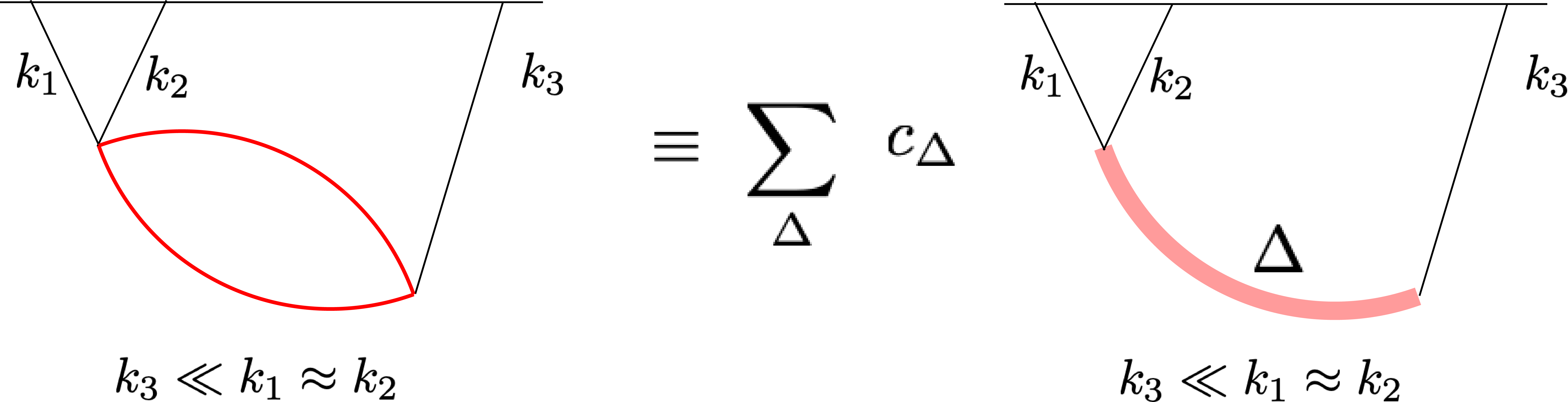
Thus from eqs. (71), (73) and (76), we will have,
| (77) | ||||
| (78) |
which can be used to get the inflaton three point function in eq. (72). We can quickly generalize this to the case of curvaton fluctuations by using eq. (64) to get,
| (79) |
Using the above and eq. (22), we derive the dimensionless three point function of the curvature perturbation,
| (80) |
Appendix B Fermion loop
To calculate the NG induced by the coupling given in eq. (68), we need the late time two point function of the type . This can be calculated by squaring and taking a trace of the spinor two point function derived in allen1986. The result is,
| (81) |
where . This matches with the answer obtained in Lu:2019tjj. We thus get using eqs. (71) and (73),
| (82) | |||
| (83) |
Using eq. (68) we can get the three point function of the curvaton fluctuations,
| (84) |
Using the above and eq. (22), the dimensionless bispectrum is given by,
| (85) |
References
- (1) D. Baumann, Inflation, in Physics of the large and the small, TASI 09, proceedings of the Theoretical Advanced Study Institute in Elementary Particle Physics, Boulder, Colorado, USA, 1-26 June 2009, pp. 523–686, 2011. arXiv:0907.5424.
- (2) Planck Collaboration, Y. Akrami et al., Planck 2018 results. X. Constraints on inflation, arXiv:1807.06211.
- (3) X. Chen and Y. Wang, Quasi-Single Field Inflation and Non-Gaussianities, JCAP 1004 (2010) 027, [arXiv:0911.3380].
- (4) D. Baumann and D. Green, Signatures of Supersymmetry from the Early Universe, Phys. Rev. D85 (2012) 103520, [arXiv:1109.0292].
- (5) V. Assassi, D. Baumann, and D. Green, On Soft Limits of Inflationary Correlation Functions, JCAP 1211 (2012) 047, [arXiv:1204.4207].
- (6) X. Chen and Y. Wang, Quasi-Single Field Inflation with Large Mass, JCAP 1209 (2012) 021, [arXiv:1205.0160].
- (7) T. Noumi, M. Yamaguchi, and D. Yokoyama, Effective field theory approach to quasi-single field inflation and effects of heavy fields, JHEP 06 (2013) 051, [arXiv:1211.1624].
- (8) S. Pi and M. Sasaki, Curvature Perturbation Spectrum in Two-field Inflation with a Turning Trajectory, JCAP 1210 (2012) 051, [arXiv:1205.0161].
- (9) J.-O. Gong, S. Pi, and M. Sasaki, Equilateral non-Gaussianity from heavy fields, JCAP 1311 (2013) 043, [arXiv:1306.3691].
- (10) N. Arkani-Hamed and J. Maldacena, Cosmological Collider Physics, arXiv:1503.08043.
- (11) H. Lee, D. Baumann, and G. L. Pimentel, Non-Gaussianity as a Particle Detector, JHEP 12 (2016) 040, [arXiv:1607.03735].
- (12) X. Chen, Y. Wang, and Z.-Z. Xianyu, Loop Corrections to Standard Model Fields in Inflation, JHEP 08 (2016) 051, [arXiv:1604.07841].
- (13) X. Chen, Y. Wang, and Z.-Z. Xianyu, Standard Model Background of the Cosmological Collider, Phys. Rev. Lett. 118 (2017), no. 26 261302, [arXiv:1610.06597].
- (14) X. Chen, Y. Wang, and Z.-Z. Xianyu, Standard Model Mass Spectrum in Inflationary Universe, JHEP 04 (2017) 058, [arXiv:1612.08122].
- (15) X. Chen, Y. Wang, and Z.-Z. Xianyu, Schwinger-Keldysh Diagrammatics for Primordial Perturbations, JCAP 1712 (2017), no. 12 006, [arXiv:1703.10166].
- (16) A. Kehagias and A. Riotto, On the Inflationary Perturbations of Massive Higher-Spin Fields, JCAP 1707 (2017), no. 07 046, [arXiv:1705.05834].
- (17) H. An, M. McAneny, A. K. Ridgway, and M. B. Wise, Quasi Single Field Inflation in the non-perturbative regime, JHEP 06 (2018) 105, [arXiv:1706.09971].
- (18) S. Kumar and R. Sundrum, Heavy-Lifting of Gauge Theories By Cosmic Inflation, JHEP 05 (2018) 011, [arXiv:1711.03988].
- (19) D. Baumann, G. Goon, H. Lee, and G. L. Pimentel, Partially Massless Fields During Inflation, JHEP 04 (2018) 140, [arXiv:1712.06624].
- (20) X. Chen, Y. Wang, and Z.-Z. Xianyu, Neutrino Signatures in Primordial Non-Gaussianities, JHEP 09 (2018) 022, [arXiv:1805.02656].
- (21) H. An, M. B. Wise, and Z. Zhang, De Sitter Quantum Loops as the origin of Primordial Non-Gaussianities, Phys. Rev. D99 (2019), no. 5 056007, [arXiv:1806.05194].
- (22) X. Chen, A. Loeb, and Z.-Z. Xianyu, Unique Fingerprints of Alternatives to Inflation in the Primordial Power Spectrum, Phys. Rev. Lett. 122 (2019), no. 12 121301, [arXiv:1809.02603].
- (23) S. Kumar and R. Sundrum, Seeing Higher-Dimensional Grand Unification In Primordial Non-Gaussianities, JHEP 04 (2019) 120, [arXiv:1811.11200].
- (24) N. Arkani-Hamed, D. Baumann, H. Lee, and G. L. Pimentel, The Cosmological Bootstrap: Inflationary Correlators from Symmetries and Singularities, arXiv:1811.00024.
- (25) L. Li, T. Nakama, C. M. Sou, Y. Wang, and S. Zhou, Gravitational Production of Superheavy Dark Matter and Associated Cosmological Signatures, JHEP 07 (2019) 067, [arXiv:1903.08842].
- (26) Y.-P. Wu, L. Yang, and A. Kusenko, Leptogenesis from spontaneous symmetry breaking during inflation, arXiv:1905.10537.
- (27) S. Alexander, S. J. Gates, L. Jenks, K. Koutrolikos, and E. McDonough, Higher Spin Supersymmetry at the Cosmological Collider: Sculpting SUSY Rilles in the CMB, arXiv:1907.05829.
- (28) S. Lu, Y. Wang, and Z.-Z. Xianyu, A Cosmological Higgs Collider, arXiv:1907.07390.
- (29) A. Hook, J. Huang, and D. Racco, Searches for other vacua II: A new Higgstory at the cosmological collider, arXiv:1907.10624.
- (30) A. Hook, J. Huang, and D. Racco, Minimal signatures of the Standard Model in non-Gaussianities, arXiv:1908.00019.
- (31) Planck Collaboration, Y. Akrami et al., Planck 2018 results. IX. Constraints on primordial non-Gaussianity, arXiv:1905.05697.
- (32) M. Alvarez et al., Testing Inflation with Large Scale Structure: Connecting Hopes with Reality, arXiv:1412.4671.
- (33) A. Moradinezhad Dizgah and C. Dvorkin, Scale-Dependent Galaxy Bias from Massive Particles with Spin during Inflation, JCAP 1801 (2018), no. 01 010, [arXiv:1708.06473].
- (34) A. Moradinezhad Dizgah, H. Lee, J. B. Muñoz, and C. Dvorkin, Galaxy Bispectrum from Massive Spinning Particles, JCAP 1805 (2018), no. 05 013, [arXiv:1801.07265].
- (35) P. D. Meerburg, M. Munchmeyer, J. B. Muñoz, and X. Chen, Prospects for Cosmological Collider Physics, JCAP 1703 (2017), no. 03 050, [arXiv:1610.06559].
- (36) P. Creminelli, On non-Gaussianities in single-field inflation, JCAP 0310 (2003) 003, [astro-ph/0306122].
- (37) C. Cheung, P. Creminelli, A. L. Fitzpatrick, J. Kaplan, and L. Senatore, The Effective Field Theory of Inflation, JHEP 03 (2008) 014, [arXiv:0709.0293].
- (38) M. Alishahiha, E. Silverstein, and D. Tong, DBI in the sky, Phys. Rev. D70 (2004) 123505, [hep-th/0404084].
- (39) D. Baumann and D. Green, Equilateral Non-Gaussianity and New Physics on the Horizon, JCAP 1109 (2011) 014, [arXiv:1102.5343].
- (40) K. Enqvist and M. S. Sloth, Adiabatic CMB perturbations in pre - big bang string cosmology, Nucl. Phys. B626 (2002) 395–409, [hep-ph/0109214].
- (41) D. H. Lyth and D. Wands, Generating the curvature perturbation without an inflaton, Phys. Lett. B524 (2002) 5–14, [hep-ph/0110002].
- (42) T. Moroi and T. Takahashi, Effects of cosmological moduli fields on cosmic microwave background, Phys. Lett. B522 (2001) 215–221, [hep-ph/0110096]. [Erratum: Phys. Lett.B539,303(2002)].
- (43) A. Loeb and M. Zaldarriaga, Measuring the small - scale power spectrum of cosmic density fluctuations through 21 cm tomography prior to the epoch of structure formation, Phys. Rev. Lett. 92 (2004) 211301, [astro-ph/0312134].
- (44) D. Wands, K. A. Malik, D. H. Lyth, and A. R. Liddle, A New approach to the evolution of cosmological perturbations on large scales, Phys. Rev. D62 (2000) 043527, [astro-ph/0003278].
- (45) S. Weinberg, Adiabatic modes in cosmology, Phys. Rev. D67 (2003) 123504, [astro-ph/0302326].
- (46) D. H. Lyth, C. Ungarelli, and D. Wands, The Primordial density perturbation in the curvaton scenario, Phys. Rev. D67 (2003) 023503, [astro-ph/0208055].
- (47) D. H. Lyth and Y. Rodriguez, The Inflationary prediction for primordial non-Gaussianity, Phys. Rev. Lett. 95 (2005) 121302, [astro-ph/0504045].
- (48) N. Bartolo, S. Matarrese, and A. Riotto, On nonGaussianity in the curvaton scenario, Phys. Rev. D69 (2004) 043503, [hep-ph/0309033].
- (49) M. Sasaki, J. Valiviita, and D. Wands, Non-Gaussianity of the primordial perturbation in the curvaton model, Phys. Rev. D74 (2006) 103003, [astro-ph/0607627].
- (50) J. M. Maldacena, Non-Gaussian features of primordial fluctuations in single field inflationary models, JHEP 05 (2003) 013, [astro-ph/0210603].
- (51) P. Creminelli and M. Zaldarriaga, Single field consistency relation for the 3-point function, JCAP 0410 (2004) 006, [astro-ph/0407059].
- (52) J. E. Kim, H. P. Nilles, and M. Peloso, Completing natural inflation, JCAP 0501 (2005) 005, [hep-ph/0409138].
- (53) K. Choi, H. Kim, and S. Yun, Natural inflation with multiple sub-Planckian axions, Phys. Rev. D90 (2014) 023545, [arXiv:1404.6209].
- (54) S. H. H. Tye and S. S. C. Wong, Helical Inflation and Cosmic Strings, arXiv:1404.6988.
- (55) I. Ben-Dayan, F. G. Pedro, and A. Westphal, Hierarchical Axion Inflation, Phys. Rev. Lett. 113 (2014) 261301, [arXiv:1404.7773].
- (56) Y. Bai and B. A. Stefanek, Natural millicharged inflation, Phys. Rev. D91 (2015), no. 9 096012, [arXiv:1405.6720].
- (57) A. de la Fuente, P. Saraswat, and R. Sundrum, Natural Inflation and Quantum Gravity, Phys. Rev. Lett. 114 (2015), no. 15 151303, [arXiv:1412.3457].
- (58) Y. Kawamura, Gauge symmetry breaking from extra space S**1 / Z(2), Prog. Theor. Phys. 103 (2000) 613–619, [hep-ph/9902423].
- (59) Y. Kawamura, Triplet doublet splitting, proton stability and extra dimension, Prog. Theor. Phys. 105 (2001) 999–1006, [hep-ph/0012125].
- (60) L. J. Hall and Y. Nomura, Grand unification in higher dimensions, Annals Phys. 306 (2003) 132–156, [hep-ph/0212134]. [,432(2002)].
- (61) B. Allen and C. A. Lütken, Spinor two-point functions in maximally symmetric spaces, Comm. Math. Phys. 106 (1986), no. 2 201–210.