Dark Matter Constraints on Low Mass and Weakly Coupled B-L Gauge Boson

Our model is based on the $U(1)_{B-L}$ extension of the SM with gauge quantum numbers under $U(1)_{B-L}$ defined by their baryon or lepton number of particles. The gauge group of the model is $SU(3)_{c}\times SU(2)_{L}\times U(1)_{Y}\times U(1)_{B-L}$, where $Y$ is the SM hypercharge. We need three right handed neutrinos (RHNs) with $B-L=-1$ to cancel the $B-L$ anomaly. The RHNs being SM singlets do not contribute to SM anomalies. The electric charge formula in this case is same as in the SM. We now add to this model a vector-like SM singlet fermion $\zeta$ with $B-L$ charge equal to $Q$. Being vector-like, this fermion does not affect the anomaly cancellation of the model. The $B-L$ group is assumed not to contribute to electric charge formula as stated in the introduction. As a result, its couplings are theoretically not restricted. We assume that there is a Higgs boson with $B-L=+2$ which gives a Majorana mass to the RHNs thereby helping to implement the seesaw mechanism for neutrino masses since the SM Higgs doublet already provides the Dirac mass to the neutrinos. The interaction Lagrangian in our model describing the interaction of the $B-L$ gauge boson (called $Z_{BL}$ here) is:

This Lagrangian is enough to derive our conclusions. We start with letting the values of $g_{BL}$, $g_{\zeta}\equiv Qg_{BL}$, $M_{Z_{BL}}$ and $m_{\zeta}$ as free parameters and explore the smaller mass range of $M_{Z_{BL}}$ and as a benchmark point, we take $m_{\zeta}$ in the range of $1$ GeV to few TeV range with $M_{Z_{BL}}<m_{\zeta}$. Clearly this covers a wide and interesting range of dark matter masses.

The only new Higgs boson in the model beyond the SM Higgs doublet, is an SM singlet field $\Delta$ with $B-L=2$. It acquires a non-zero vacuum expectation value $\langle\Delta\rangle=v_{BL}$. The real part of $\Delta$ is a physical Higgs field, which we denote by $\sigma$. It couples to the right handed neutrinos which we assume heavy (in the TeV range or higher) so that $\sigma$ could be a long lived particle. Also it has no direct couplings to quarks and leptons and such couplings arise from its mixing with the SM Higgs boson. For a GeV mass $\sigma$, we may expect this mixing to be of order $m_{\sigma}^{2}/m_{h}^{2}\sim 10^{-2}$. Due to this small coupling, its production cross section in lepton as well as hadron colliders is very small. Further discussion of the phenomenology of this new Higgs boson is beyond the scope of this paper. In fact, in a recent paper nobu2, we have argued that for some parameter ranges of the theory, the $\sigma$ particle can be a decaying dark matter of the universe.

As far as other phenomenology of the model is concerned, we note that for $g^{2}_{BL}/M^{2}_{Z_{BL}}\lesssim 10^{-6}$ GeV^-2, the neutral current and other low energy constraints are automatically satisfied (see Table 8.13 of reference LEP_rev). This limit broadly satisfies all the LEP constraints for $VV$ type current couplings. It also implies that $g_{BL}\lesssim 10^{-3}\,M_{Z_{BL}}[{\rm GeV}]$ is allowed by low energy observations and we seek other constraints in this domain when a dark matter is included in the theory. There are also ATLAS upper bounds on $g_{BL}$ as a function of $M_{Z_{BL}}$ but this bound for low mass $Z_{BL}$ is in the range of $g_{BL}\leq 2\times 10^{-3}$ or so ATLbound for $M_{Z_{BL}}$ about a GeV and it becomes weaker as we go to higher masses. See also the review Lang.

We also note that our model is different from other $U(1)^{\prime}$ models since in our case the $Z_{BL}$ coupling with quarks and leptons is specified by the $B-L$ charges of the fermions. One the other hand, the DM field has an arbitrary $B-L$ charge $Q$ and we investigate the phenomenological viability of our model for a wide range of the parameter space from $|Q|\ll 1$ to $|Q|\gg 1$.

We first consider the case where the parameter range of the model is such that $\zeta$ is a thermal dark matter. We will find these parameter ranges and their possible implications below. This is the case where both $g_{BL}$ and $g_{\zeta}$ have such values that $Z_{BL}$, $\zeta$ and SM particles were all in thermal equilibrium in the early universe, followed by the dark matter decoupling which leads to the DM relic density.

We first note that the dark matter interacts with the SM particle only via the $B-L$ gauge interactions. The Higgs boson field that breaks $B-L$ does not couple to the dark matter particle due to their $B-L$ charge mismatch and therefore does not contribute to the thermal equilibrium consideration between $\zeta$ and SM particles.

For the Dirac DM particle $\zeta$ to be a thermal dark matter, whose relic abundance is determined by thermal freeze-out, it must be in thermal equilibrium with the SM particles as well as the $Z_{BL}$ in the very early universe. As the temperature of the universe drops below the $m_{\zeta}$, the Boltzmann suppression makes the $\zeta$ particle density low and it goes out of equilibrium. After thermal freeze-out occurs, the DM freely expands till the current epoch and forms the dark matter of the universe. Its current abundance is determined by the values of $g_{BL}$, $g_{\zeta}$ and $m_{\zeta}$.

Typically in a thermal freeze-out situation, the fact that at one point the $\zeta$ particle was in equilibrium implies constraints on the parameters $g_{\zeta}$. We have to consider different processes that can keep $\zeta$ particles in equilibrium with the SM particles. The first one is via direct process ${\zeta\bar{\zeta}\to f\bar{f}}$ mediated by $Z_{BL}$, which leads to

where $n_{\zeta}(T)=\frac{3\zeta(3)}{\pi^{2}}T^{3}$ is the DM number density for $T\gtrsim m_{\zeta}$, $g_{*}$ is the effective number of degrees of freedom for SM particles in thermal equilibrium (we set $g_{*}=106.75$ in the following analysis), and $M_{P}=2.43\times 10^{18}$ GeV is the reduced Planck mass. Since we are interested in a low mass $Z_{BL}$ boson, we obtain $\langle\sigma v\rangle\simeq\frac{g^{2}_{BL}g^{2}_{\zeta}}{4\pi T^{2}}$ for the $\zeta\bar{\zeta}\to f\bar{f}$ process, independently of the $Z_{BL}$ mass. Requiring the thermal equilibrium condition to be satisfied at $T\simeq m_{\zeta}$, we obtain the following constraint on the gauge coupling parameters:

As we will see in the next subsection, the above thermal equilibrium condition is not consistent with the direct DM detection constraints which are very severe for low $M_{Z_{BL}}$.

The second possibility for $\zeta$ to be in equilibrium with the SM particles is via a two step process: in the first step $Z_{BL}$ comes to equilibrium with SM fermions via the process $f\bar{f}\to Z_{BL}\gamma$ and then $\zeta$ goes into equilibrium with $Z_{BL}$ and hence with the SM fermions via the process $Z_{BL}Z_{BL}\to\zeta\zeta$. The thermal equilibrium condition for the first process is

where $n_{Z_{BL}}(T)=\frac{2\zeta(3)}{\pi^{2}}T^{3}$ is the number density of $Z_{BL}$, and $\langle\sigma v\rangle_{f\bar{f}\to Z_{BL}\gamma}\simeq\frac{g_{BL}^{2}\alpha_{e}}{T^{2}}$ with the fine-structure constant of $\alpha_{e}=1/128$. We require that this condition is satisfied at $T=m_{\zeta}$ (at latest) and obtain

The second process depends only on $g_{\zeta}$ and the equilibrium condition gives a lower bound on $g_{\zeta}\geq 9.2\times 10^{-5}\,\left(m_{\zeta}[{\rm GeV}]\right)^{1/4}$ by using $\langle\sigma v\rangle_{Z_{BL}Z_{BL}\to\zeta\bar{\zeta}}\simeq\frac{g_{\zeta}^{4}}{16\pi T^{2}}$ in Eq. (4). Clearly if we want to get the DM relic density right, we need a larger $g_{\zeta}$ and therefore it is in our acceptable range for the DM relic density, $\zeta$ is in thermal equilibrium with $Z_{BL}$. Note that the processes $Z_{BL}\to ff$ and $ff\to Z_{BL}$ which apparently are not suppressed by electromagnetic coupling, are expected to be phase space suppressed instead; so we do not consider them here.

Next, we discuss the DM relic density constraints on the model. To evaluate the DM relic density, we solve the Boltzmann equation given by

where $x=m_{\zeta}/T$ is the inverse “temperature” normalized by the DM mass $m_{\zeta}$, $\langle\sigma v\rangle$ is a thermally averaged DM annihilation cross section ($\sigma$) times relative velocity ($v$), $H(m_{\zeta})$ is the Hubble parameter at $T=m_{\zeta}$, $s(m_{\zeta})$ is the entropy density of the thermal plasma at $T=m_{\zeta}$, $Y$ is the yield of the DM particle which is defined as a ratio of the DM number density to the entropy density, and $Y_{EQ}$ is the yield of the DM in thermal equilibrium. Explicit forms for the quantities in the Boltzmann equation are as follows:

where $K_{2}(x)$ is the modified Bessel function of the second kind, and $g_{DM}=4$ is the number of degrees of freedom for the Dirac fermion DM particle $\zeta$.

The thermal average of the DM annihilation cross section is given by the following integral expression:

where $n_{EQ}=s(m_{\zeta})Y_{EQ}/x^{3}$ is the DM number density, and $K_{1}$ is the modified Bessel function of the first kind. The DM annihilation occurs via the process $\zeta\bar{\zeta}\to Z_{BL}Z_{BL}$ for $m_{\zeta}>M_{Z_{BL}}$. In our considerations above, we have ignored the inverse decay process $\zeta\bar{\zeta}\to Z_{BL}$, since it is a small contribution at high temperatures, suppressed by a very small volume of the phase space. We have also not taken into account the Sommerfeld enhancement. Typically, Sommerfeld enhancement is significant if the DM speed is very low and bound states of $\zeta$-$\bar{\zeta}$ are formed with a large $g_{\zeta}$ value. In our freeze-out scenario, the annihilation cross section in the early universe uses the speed $v\sim 0.05$ or so and the coupling is not so large (see Eq. (13)). Similarly, the condition for DM bound state formation is not satisfied. We estimate the Sommerfeld enhancement factor to be therefore small at the freeze-out epoch. However, at the recombination and the current epoch, Sommerfeld effect is significant due to very low velocities of DM particles and leads to important constraints on the parameters for the freeze-out case (see below). By solving the Boltzmann equation of Eq. (8) with the initial condition $Y(x)=Y_{EQ}(x)$ for $x\ll 1$, we evaluate the DM yield at present, $Y(x\to\infty)$. The relic abundance of the DM in the present universe is then given by

where $s_{0}=2890$ cm^-3 is the entropy density of the present Universe, and $\rho_{c}/h^{2}=1.05\times 10^{-5}$ GeV/cm³ is the critical density. For the thermal DM scenario, the asymptotic solution of the Boltzmann equation ($Y(\infty)$) is known, and with a good accuracy, the thermal DM relic density is expressed to be review1; review2

where $M_{P}$ and $\langle\sigma v\rangle$ are evaluated in units of GeV, the freeze-out temperature of the DM particle is approximately evaluated as $x_{f}=m_{\zeta}/T_{f}\simeq\ln(x)-0.5\ln(\ln(x))$ with $x\simeq 0.19\sqrt{g_{DM}/g_{*}}M_{P}\,m_{\zeta}\,\langle\sigma v\rangle$. Since the annihilation process occurs via $s$-wave, we can approximate $\langle\sigma v\rangle$ as $\sigma v$ in the non-relativistic limit. Here in our analysis, we employ Eqs. (32) and (29) given in Appendix for the annihilation processes $\zeta\bar{\zeta}\to Z_{BL}Z_{BL}$ and $\zeta\bar{\zeta}\to f\bar{f}$, respectively. As we will discuss in the following subsection, the direct DM detection constraints are very severe and we find that they require $g_{BL}\ll g_{\zeta}$. Thus, the contribution from the process $\zeta\bar{\zeta}\to f\bar{f}$ is negligibly small.

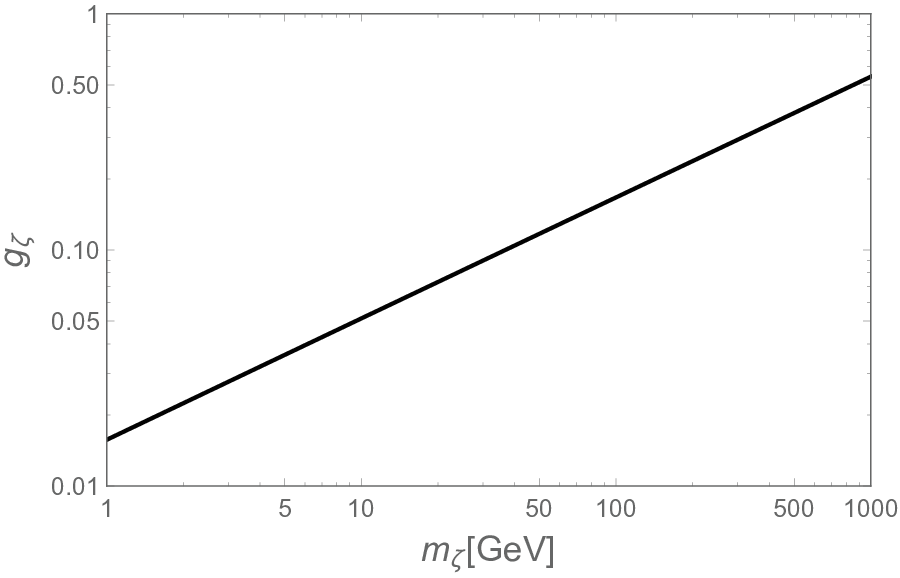
In order to reproduce the observed DM relic density at the present epoch, $\Omega_{DM}h^{2}=0.12$ Planck2019, we obtain a relation between the DM mass and the DM coupling with $Z_{BL}$ for $M^{2}_{Z_{BL}}\ll m^{2}_{\zeta}$, which is shown by the line in Fig. 1. The observed DM relic density is reproduced along the line, which we find to be well approximated by

As we expected, the thermal equilibrium condition for the process $Z_{BL}Z_{BL}\leftrightarrow\zeta\bar{\zeta}$ we have found before (see after Eq. (7)) is always satisfied for $m_{\zeta}>1$ GeV. In Fig. 2, we show the relation between the $Z_{BL}$ mass and the DM coupling with $Z_{BL}$ for fixed DM masses of 2 GeV (black), 10 GeV (red), 100 GeV (blue), and 500 GeV (green). The observed DM relic density is reproduced along each line. We can see that the coupling is almost constant for a fixed DM mass for $M^{2}_{Z_{BL}}\ll m^{2}_{\zeta}$ and is well-approximated by Eq. (13). The coupling is sharply rising when the $Z_{BL}$ mass becomes very close to the DM mass because of the phase space/kinematic effect.

Let us now turn to the direct detection constraints. In Fig. 3, we show the current upper bound on the spin-independent cross section ($\sigma_{SI}$) for the elastic scattering of the DM particle with a nucleon for the DM mass of $m_{DM}\geq 2$ GeV. For the DM mass $m_{DM}\geq 6$ GeV, the most stringent upper bound is obtained by XENON1T experiment Xenon1T-2018 while for $2\,{\rm GeV}\leq m_{DM}\leq 6$ GeV, the upper bound is obtained by a combination of DarkSide-50 DarkSide-50, LUX LUX-2019 and PandaX-II PandaX-II. As is well known the constraints are most severe for a DM mass around 30 GeV and become weaker on either side of this mass.

In our model, the elastic scattering of the DM particle with a nucleon $\zeta N\to\zeta N$ occurs via the exchange of $Z_{BL}$ boson. The cross section for the process is given by farinaldo

where $\mu_{\zeta N}=m_{\zeta}m_{N}/(m_{\zeta}+m_{N})$ is the reduced mass for the DM-nucleon system with $m_{N}=0.983$ GeV being the nucleon mass. Note that this cross section formula is valid for $M_{Z_{BL}}^{2}\gtrsim M_{T}E_{R}$, where $M_{T}$ is a target nuclei mass, and $E_{R}$ is a typical recoil energy. For XENON1T experiment, $M_{T}\sim 100$ GeV and $E_{R}\sim 10$ keV, so that we can apply Eq. (14) for $M_{Z_{BL}}\gtrsim 50$ MeV. As $M_{Z_{BL}}$ decreases from $M_{Z_{BL}}=50$ MeV, the $Z_{BL}$ exchange process becomes long-range and $\sigma_{SI}$ quickly approaches a constant value as shown in Refs. DelNobile:2015uua; DelNobile:2015bqo; Panci:2014gga; Li:2014vza. For $M_{Z_{BL}}<50$ MeV, we approximate the constant cross section by Eq. (14) with $M_{Z_{BL}}=50$ MeV fixed. For a given $m_{\zeta}$, say, one GeV, which satisfies all the above constraints, we see that as $M_{Z_{BL}}$ goes down, the cross section rises in Eq. (14). Since $g_{BL}$ has a lower bound from Eq. (7) and $g_{\zeta}$ values are already fixed, this implies a lower bound on $M_{Z_{BL}}$ depending on the $\zeta$ mass along the upper bound on $\sigma_{SI}$ in Fig. 3. This lower bound is shown as the black solid line in Fig. 4. For example, for $m_{\zeta}=2$ GeV, we find the minimum $Z_{BL}$ mass to be $\simeq 50$ MeV.

In our model, the dark matter annihilation to $Z_{BL}Z_{BL}$ at late time can undergo Sommerfeld enhancement due to the low velocity of DM fermion. The $Z_{BL}$s can subsequently decay to SM fermions, which can lead to signals in indirect DM searches such as the CMB measurement and AMS-02 anti-proton searches. These constraints have been analyzed in Refs. walia; cirelli and they lead to very tight constraints on DM mass in the range of 1 GeV to 100 GeV. Even though the Ref. cirelli considers a dark photon portal, it is very similar to our $B-L$ portal and therefore we can apply their constraints to our case. In Fig. 4, we have combined the direct detection constraint with the indirect detection constraints obtained in Ref. cirelli. The green region is allowed by all the constraints and this pretty much rules out the low mass (thermal) DM scenario for $m_{Z_{BL}}\lesssim 10$ GeV.

This case arises when the gauge couplings $g_{BL}$ and $g_{\zeta}$ have much smaller values than the freeze-out case so that the dark matter particle was never in equilibrium with the thermal plasma of the SM particles. In this section, we assume that the $\zeta$ particle had zero initial abundance at the reheating after inflation. Productions of $\zeta$ particles from inflaton decay will be briefly discussed in Sec. V. There are then two possible cases:

(A) the $Z_{BL}$ was in thermal equilibrium with SM particles. This corresponds to the case where $g_{BL}\geq 2.7\times 10^{-8}\sqrt{m_{\zeta}[{\rm GeV}]}$, and

(B) the $Z_{BL}$ was not in thermal equilibrium with SM particles i.e. $g_{BL}<2.7\times 10^{-8}\sqrt{m_{\zeta}[{\rm GeV}]}$.

Next, we proceed to evaluate the DM relic abundance by numerically solving the Boltzmann equation in Eq. (8). Note that even for the freeze-in case the Boltzmann equation is of the same form as in the thermal dark matter case. This is because the term proportional to $Y_{EQ}^{2}$ in the right-hand side of Eq. (8) corresponds to the DM particle productions from the SM thermal plasma. The difference from the thermal dark matter case is that we set the boundary condition for the freeze-in case to be $Y(x_{RH})=0$, where $x_{RH}=m_{\zeta}/T_{RH}\ll 1$ is related to the reheat temperature ($T_{RH}$) after inflation. The relic abundance of the DM in the present universe is given in Eq. (11).

In evaluating the thermal average of the DM annihilation cross section in Eq. (10), we consider two processes for the DM particle creation, $f\bar{f}\to\zeta\bar{\zeta}$ mediated by $Z_{BL}$ and $Z_{BL}Z_{BL}\to\zeta\bar{\zeta}$. Note that the second process is active only for case (A) (except for a special case, sequential freeze-in, that we discuss below). The corresponding cross sections are given by those of the DM annihilation processes. In Appendix, we list the exact cross section formulas for the processes. Using them for Eq. (10), we evaluate the thermal average of the cross section and then numerically solve the Boltzmann equation of Eq. (8) with the boundary condition of $Y(x_{RH})=0$. In the freeze-in mechanism, the DM particles are created mostly in the relativistic regime, $T\gg m_{\zeta}$, where the annihilation cross sections are approximately given by (see Eqs. (30) and (33) in Appendix)

where we have assumed $m_{b}^{2}\ll m_{\zeta}^{2}<m_{t}^{2}$ and $m_{Z_{BL}}^{2}\ll m_{\zeta}^{2}$. Although we use the exact cross section formulas to evaluate $Y(x)$ in our analysis, we find that the approximation formulas in Eq. (17) lead to almost the same results as those obtained by the exact formulas.

In Fig. 5, fixing $m_{\zeta}=30$ GeV, we show the resultant $Y(x)$ for two cases: One is for $g_{\zeta}^{2}g_{BL}^{2}=8.2\times 10^{-24}$ with $g_{BL}\gg g_{\zeta}$ (solid line), and the other is $g_{\zeta}^{4}=1.2\times 10^{-23}$ with $g_{BL}\ll g_{\zeta}$ (dashed line). For the first case, the process $\zeta\bar{\zeta}\to f\bar{f}$ dominates, while the process $\zeta\bar{\zeta}\to Z_{BL}Z_{BL}$ dominates for the second case. As we can see, $Y(x)$ grows from $Y(x_{RH}\ll 1)=0$ and becomes constant at $x\simeq 1$. Using the approximation formulas in Eq. (17), this behavior can be qualitatively understood as follows: In the first case, for $x\lesssim 1$, we have $\langle\sigma v\rangle\propto g_{\zeta}^{2}\,g_{BL}^{2}(x^{2}/m_{\zeta}^{2})$, and Eq. (8) can be easily solved with $Y\ll Y_{EQ}\simeq$ constant and $Y(x_{RH}\ll 1)=0$. We find a solution to be $Y(x)\propto g_{\zeta}^{2}g_{BL}^{2}(x-x_{RH})/m_{\zeta}\simeq g_{\zeta}^{2}\,g_{B}^{2}(x/m_{\zeta})$. Since the DM particle creation from the thermal plasma should stop at $T\sim m_{\zeta}$ because of the kinematics, $Y(\infty)\sim Y(x\simeq 1)\propto g_{\zeta}^{2}g_{BL}^{2}/m_{\zeta}$. Using Eq. (11), we find that the resultant DM relic density is proportional to $g_{\zeta}^{2}\,g_{B}^{2}$ while independent of the DM mass. We have arrived at the same conclusion even for the numerical result by using the exact cross section formulas. We find a similar result for the second case, namely, the resultant DM relic density is proportional to $g_{\zeta}^{4}$ while independent of the DM mass.

By numerically solving the Boltzman equation, we find that independently of $m_{\zeta}$, the observed DM relic density of $\Omega_{DM}h^{2}=0.12$ is reproduced in case (A) by

In case (B), on the other hand, there is no $Z_{BL}$ initially, the condition is given by only the first term in the above equation, i.e.

For example, for $m_{\zeta}=1$ GeV, the first equation implies that $g_{\zeta}\sim 10^{-6}$ or lower whereas the second case corresponds to $g_{\zeta}\sim 10^{-4}$ or higher.

Very recently, it has been pointed out in Ref. Hambye:2019dwd that in case (B) “sequential freeze-in” can dominantly produce the DM particles compared to the process of $f\bar{f}\to\zeta\bar{\zeta}$ considered above. If this is the case, Eq. (19) is not the right condition to reproduce $\Omega_{DM}\,h^{2}=0.12$. In the case of sequential freeze-in, the DM particles are produced in two steps. First, $Z_{BL}$ is produced from the thermal plasma of the SM particles, and then the DM particles are produced through $Z_{BL}Z_{BL}\to\zeta\bar{\zeta}$. Let us now estimate the DM relic density through the sequential freeze-in. The yield of $Z_{BL}$ ($Y_{Z_{BL}}$) is calculated by the Boltzmann equation,

where $Y^{EQ}_{Z_{BL}}\simeq Y^{EQ}_{\gamma}\simeq 5.2\times 10^{-3}$ are the yields of $Z_{BL}$ and the photon, respectively, in the thermal equilibrium, and $\langle\sigma v\rangle_{f\bar{f}\to Z_{BL}\gamma}\simeq\frac{g_{BL}^{2}\alpha_{e}}{m_{\zeta}^{2}}x^{2}$. This Boltzmann equation is easily solved from $x_{RH}\ll 1$, and we find

for $x\lesssim m_{\zeta}/M_{Z_{BL}}$. With this $Y_{Z_{BL}}(x)$, we calculate the DM density by solving the Boltzmann equation,

where we have used $\langle\sigma v\rangle_{Z_{BL}Z_{BL}\to\zeta\bar{\zeta}}(Y_{Z_{BL}}^{EQ})^{2}=\langle\sigma v\rangle_{\zeta\bar{\zeta}\to Z_{BL}Z_{BL}}\,Y_{EQ}^{2}$ in the second line. In our analysis here, we have assumed that the sequential freeze-in dominates and neglected the DM pair production process $f\bar{f}\to\bar{\zeta}\zeta$ from the thermal plasma.

For fixed values of $g_{BL}$, $g_{\zeta}$ and $m_{\zeta}$, we numerically solve Eq. (22) from $x_{RH}\ll 1$. In Fig. 6, we show the yield of the Dirac DM particle as a function of $x=m_{\zeta}/T$ for $m_{\zeta}=30$ GeV (solid line), along with the yield of $Z_{BL}$ (dashed line). Here, we have taken $g_{BL}=5.0\times 10^{-10}$ and $g_{\zeta}=6.3\times 10^{-4}$. We can see the result similar to that in Fig. 5. As we can understand from Eq. (21) and Eq. (31), $Y(\infty)\sim Y(x=1)\propto g_{\zeta}^{4}\,g_{BL}^{4}/m_{\zeta}^{2}$. We find that the observed DM relic density of $\Omega_{DM}h^{2}=0.12$ is reproduced when

Comparing this result with Eq. (19), we conclude that the sequential freeze-in dominantly produces the DM particles for $m_{\zeta}<2.5$ TeV, in case (B). For $m_{\zeta}=30$ GeV, our result is displayed in Fig. 7. The plots show cusps at $g_{BL}\simeq 1.5\times 10^{-7}$, which is the boundary value to separate case (A) and case (B). To simplify our analysis, we have calculated the two cases separately by considering only the dominant process in each case. Because of this simplification, the cusps appear in our results, and they will be smoothed away if we take all terms into account in the Boltzmann equations.

Thus to summarize, for the freeze-in scenario, there are the following constraints on parameters to reproduce the observed DM relic density depending on the ranges of $B-L$ gauge coupling $g_{BL}$ and dark matter mass $m_{\zeta}$. Case (A): This constraint applies for the parameter region $g_{BL}\geq 2.7\times 10^{-8}\sqrt{m_{\zeta}[{\rm GeV}]}$ where one has $g^{2}_{\zeta}\,g^{2}_{BL}+\frac{0.82}{1.2}\,g^{4}_{\zeta}\simeq 8.2\times 10^{-24}$ to reproduce $\Omega_{DM}\,h^{2}=0.12$. Case (B): for $g_{BL}<2.7\times 10^{-8}\sqrt{m_{\zeta}[{\rm GeV}]}$, there are two separate constraints depending on $m_{\zeta}$. Case (B1): for $m_{\zeta}\lesssim 2.5$ TeV, we find $g_{\zeta}^{2}\,g_{BL}^{2}\simeq 8.2\times 10^{-24}\,\left(\frac{m_{\zeta}}{2.5\,{\rm TeV}}\right)$ and in case (B2): for $m_{\zeta}\gtrsim 1.5$ TeV, we find $g_{\zeta}^{2}\,g_{BL}^{2}\simeq 8.2\times 10^{-24}$.

We now discuss possible probes of the freeze-in scenario in the laboratory. There are several experiments that can probe various parameter ranges of the model. This is shown in Fig. 8. The relevant experiments are those at the ones attempting to extend lifetime frontier of various new weakly coupled beyond the SM particles. They typically look for displaced vertices. The experiments are FASER and SHiP at the LHC; Belle II andLHCb as well as LDMX experiment proposed to search for weakly coupled light DM particles.

The planned FASER detector faser at the LHC will probe the low $M_{Z_{BL}}$ ($\leq 1-2$ GeV) and low $g_{BL}$ region of the theory. This is a detector which will be installed in a tunnel near the ATLAS detector about 480 meters away to look for displaced vertices with charged particles from long-lived charge-neutral particles produced at the primary LHC vertex. In the very low $g_{BL}$ range, our model falls into this category since due to low $g_{BL}$ and low mass $M_{Z_{BL}}$, the distance travelled by a highly boosted $Z_{BL}$ before decaying is given by $c\tau\sim\frac{12\pi E_{Z_{BL}}}{g^{2}_{BL}M_{Z_{BL}}^{2}}$ and experiments such as FASER searching for displaced vertices can give useful constraints.

In Fig. 8, the horizontal solid lines correspond to the results for the various $B-L$ charges of the DM particle, $Q=2\times 10^{-4}$, $5\times 10^{-3}$, $0.1$, $1.01$ (black line), $5$, and $50$ from top to bottom. Along the horizontal lines, $\Omega_{DM}\,h^{2}=0.12$ is satisfied. Various planned and proposed experiments and their search reaches are indicated (see Ref. faser for details) and the current excluded region is gray-shaded Bauer:2018onh. The blue shaded region at top-left corner is excluded by the XENON1T results. As discussed in Sec. III.2, $\sigma_{SI}$ becomes constant for $M_{Z_{BL}}\lesssim 50$ MeV, and we find that the XENON1T bound is satisfied for $g_{BL}\lesssim 8.9\times 10^{-7}$ for any values of $M_{Z_{BL}}$. Even for the freeze-in case, the direct DM detection experiments provide very severe constraints and exclude a part of the open window. From Fig. 8, we see that various Lifetime Frontier experiments in the near future can test our freeze-in scenario.

If $Z_{BL}$ mass is less than 100 MeV, it can be produced from $e^{+}e^{-}$ and $\nu\bar{\nu}$ collisions in the supernova, whose core temperature is believed to be 30 MeV. To avoid any constraints on $g_{BL}$ from energy loss considerations of SN 1987A, we stay above $Z_{BL}$ mass of 200 MeV.

Coming to constraints from Big Bang nucleosynthesis, we assume that the RHNs required for anomaly cancellation acquire heavy Majorana mass ($M_{N_{R}}\geq 100$ GeV or more) so that the only new degree of freedom we have to consider at the epoch of BBN are the three modes of the vector boson $Z_{BL}$ (two transverse and one longitudinal). We assume $M_{Z_{BL}}$ to be in the one GeV or lower range but above 200 MeV. For the higher mass range, as long as $Z_{BL}$ is in thermal equilibrium, the $Z_{BL}$ density at decoupling is already suppressed enough so that there are no BBN constraints.

The physics of our considerations in the lower mass range are as follows: if the gauge coupling is large enough that the $Z_{BL}$ is in thermal equilibrium till $T=1$ MeV, then how much it contributes to the quantity $\Delta N_{eff}$ depends on its mass. If its mass is larger than 10 MeV, its abundance at $T=1$ MeV will be Boltzmann suppressed and its contributions to energy density will be within the current $\Delta N_{eff}$ limits. Since we are interested in the mass range of 200 MeV or more to avoid supernova constraints, we need not worry about the BBN constraints unless the gauge coupling is below $10^{-10}$ GeV in which case it can survive till $T\sim 1$ MeV and affect BBN. The limit of $10^{-10}$ comes from requiring that $\Gamma_{Z_{BL}}\sim H(T=1{\rm MeV})$.

References

- (1) R. E. Marshak and R. N. Mohapatra, Phys. Lett. 91B, 222 (1980).
- (2) R. N. Mohapatra and R. E. Marshak, Phys. Rev. letters 44, 1316 (1980).
- (3) A. Davidson, Phys. Rev. D 20, 776 (1979).
- (4) W. Buchmuller, C. Greub and P. Minkowski, Phys. Lett. B 267, 395 (1991).
- (5) S. Khalil, J. Phys. G 35, 055001 (2008).
- (6) L. Basso, arXiv:1106.4462 [hep-ph].
- (7) L. Basso, A. Belyaev, S. Moretti and C. H. Shepherd-Themistocleous, Phys. Rev. D 80, 055030 (2009).
- (8) S. Iso, N. Okada and Y. Orikasa, Phys. Lett. B 676, 81 (2009); Phys. Rev. D 80, 115007 (2009).
- (9) A. A. Abdelalim, A. Hammad and S. Khalil, Phys. Rev. D 90, no. 11, 115015 (2014)
- (10) A. Biswas, S. Choubey and S. Khan, JHEP 1808, 062 (2018)
- (11) P. Minkowski, Phys. Lett. B 67, 421 (1977).
- (12) R. N. Mohapatra and G. Senjanović, Phys. Rev. Lett. 44, 912 (1980).
- (13) T. Yanagida, Conf. Proc. C 7902131, 95 (1979).
- (14) M. Gell-Mann, P. Ramond and R. Slansky, Conf. Proc. C 790927, 315 (1979) [arXiv:1306.4669 [hep-th]].
- (15) S. L. Glashow, NATO Sci. Ser. B 61, 687 (1980).
- (16) G. Chauhan, P. S. B. Dev, R. N. Mohapatra and Y. Zhang, JHEP 1901, 208 (2019).
- (17) P. Fileviez Perez, C. Murgui and A. D. Plascencia, Phys. Rev. D 100, 035041 (2019).
- (18) P. H. Gu, arXiv:1907.10018 [hep-ph].
- (19) C. P. Burgess, J. P. Conlon, L. Y. Hung, C. H. Kom, A. Maharana and F. Quevedo, JHEP0807, 073 (2008).
- (20) L. J. Hall, K. Jedamzik, J. March-Russell and S. M. West, JHEP 1003, 080 (2010).
- (21) N. Bernal, M. Heikinheimo, T. Tenkanen, K. Tuominen and V. Vaskonen, Int. J. Mod. Phys. A 32, no. 27, 1730023 (2017).
- (22) T. Hambye, M. H. G. Tytgat, J. Vandecasteele and L. Vanderheyden, Phys. Rev. D 98, no. 7, 075017 (2018).
- (23) X. Chu, T. Hambye and M. H. G. Tytgat, JCAP 1205, 034 (2012).
- (24) K. Kaneta, Z. Kang and H. S. Lee, JHEP 1702, 031 (2017).
- (25) A. Albert et al. 1611.03184, [Astro-ph.HE]
- (26) M. Bauer, P. Foldenauer and J. Jaeckel, JHEP 1807, 094 (2018).
- (27) A. Biswas and A. Gupta, JCAP 1609, 044 (2016)
- (28) J. Heeck, Phys. Lett. B 739, 256 (2014).
- (29) M. Dutra, M. Lindner, S. Profumo, F. S. Queiroz, W. Rodejohann and C. Siqueira, JCAP 1803, 037 (2018).
- (30) M. Cirelli, P. Panci, K. Petraki, F. Sala and M. Taoso, JCAP 1705, 036 (2017).
- (31) J. L. Feng, I. Galon, F. Kling and S. Trojanowski, Phys. Rev. D 97, no. 3, 035001 (2018) [arXiv:1708.09389 [hep-ph]].
- (32) R. N. Mohapatra and N. Okada, Phys. Rev. D 101, 115022 (2020).
- (33) Electroweak [LEP and ALEPH and DELPHI and L3 and OPAL Collaborations and LEP Electroweak Working Group and SLD Electroweak Group and SLD Heavy Flavor Group], hep-ex/0312023.
- (34) M. Aaboud et al. [ATLAS Collaboration], JHEP 1710, 182 (2017).
- (35) Paul Langacker, Rev. Mod. Phys. 81, 1199 (2009).
- (36) A. Alves, A. Berlin, S. Profumo and F. S. Queiroz, JHEP 1510, 076 (2015); Phys. Rev. D 92, no. 8, 083004 (2015).
- (37) E. W. Kolb and M. S. Turner, Front. Phys. 69, 1 (1990).
- (38) G. Bertone, D. Hooper and J. Silk, Phys. Rept. 405, 279 (2005)
- (39) N. Aghanim et al. [Planck Collaboration], arXiv:1807.06209 [astro-ph.CO].
- (40) E. Aprile et al. [XENON Collaboration], Phys. Rev. Lett. 121, no. 11, 111302 (2018).
- (41) P. Agnes et al. [DarkSide Collaboration], Phys. Rev. Lett. 121, no. 8, 081307 (2018).
- (42) D. S. Akerib et al. [LUX Collaboration], arXiv:1907.06272 [astro-ph.CO].
- (43) X. Cui et al. [PandaX-II Collaboration], Phys. Rev. Lett. 119, no. 18, 181302 (2017).
- (44) E. Del Nobile, M. Kaplinghat and H. B. Yu, JCAP 1510, 055 (2015) doi:10.1088/1475-7516/2015/10/055 [arXiv:1507.04007 [hep-ph]].
- (45) E. Del Nobile, M. Nardecchia and P. Panci, JCAP 1604, 048 (2016).
- (46) P. Panci, Adv. High Energy Phys. 2014, 681312 (2014).
- (47) T. Li, S. Miao and Y. F. Zhou, JCAP 1503, 032 (2015).
- (48) T. Bringmann, F. Kahlhoefer, K. Schmidt-Hoberg and P. Walia, Phys. Rev. Lett. 118, no. 14, 141802 (2017)
- (49) T. Hambye, M. H. G. Tytgat, J. Vandecasteele and L. Vanderheyden, Phys. Rev. D 100, no. 9, 095018 (2019) [arXiv:1908.09864 [hep-ph]].
- (50) A. Ariga et al. [FASER Collaboration], Phys. Rev. D 99, no. 9, 095011 (2019).
- (51) S. Alekhin et al., Rept. Prog. Phys. 79, no. 12, 124201 (2016).
- (52) T. Akesson et al. [LDMX Collaboration], arXiv:1808.05219 [hep-ex].
- (53) M. J. Dolan, T. Ferber, C. Hearty, F. Kahlhoefer, and K. Schmidt-Hoberg, JHEP 12, 094 (2017).
- (54) P. Ilten, J. Thaler, M. Williams, and W. Xue, Phys. Rev. D92, no. 11, 115017 (2015).
- (55) P. Ilten, Y. Soreq, J. Thaler, M. Williams, and W. Xue, Phys. Rev. Lett. 116 no. 25, 251803 (2016).
- (56) M. Bauer, P. Foldenauer and J. Jaeckel, JHEP 1807, 094 (2018) [JHEP 2018, 094 (2020)].
- (57) S. Heeba and F. Kahlhoefer, arXiv:1908.09834 [hep-ph].