Dissipativity analysis of negative resistance circuits
Abstract
This paper deals with the analysis of nonlinear circuits that interconnect passive elements (capacitors, inductors, and resistors) with nonlinear resistors exhibiting a range of negative resistance. Such active elements are necessary to design circuits that switch and oscillate. We generalize the classical passivity theory of circuit analysis to account for such non-equilibrium behaviors. The approach closely mimics the classical methodology of (incremental) dissipativity theory, but with dissipation inequalities that combine signed storage functions and signed supply rates to account for the mixture of passive and active elements.
keywords
Nonlinear circuits; Dissipative systems; Active elements; Limit cycles; Bistability.footnoteinfo]The research leading to these results has received funding from the European Research Council under the Advanced ERC Grant Agreement Switchlet n.670645.
, ,
1 Introduction
The concept of passivity is a foundation of circuit theory [1]. It led to the generalized concept of dissipativity [35], [36], which has become a foundation of nonlinear system theory [18, 33]. Yet the applications of nonlinear system theory have been dominated by mechanical and electro-mechanical systems [6], [12], [27], [30], with significantly less attention to nonlinear circuits [5, 7].
Starting with the seminal work of Chua [9] and the textbook of Chua and Desoer [10], the research on nonlinear circuits has somewhat diverged from the research on nonlinear dissipative systems. The emphasis in nonlinear circuit theory has been on non-equilibrium behaviors whereas the focus of dissipativity theory is an interconnection framework for systems that converge to equilibrium.
Negative resistance devices are the essence of non-equilibrium behaviors such as switches [8], [17], [22], nonlinear oscillations [19], [23], or chaotic behavior [21], [29]. In contrast, dissipativity theory is a stability theory for physical systems that only dissipate energy and that relax to equilibrium when disconnected from an external source of energy.
The present paper is a step towards generalizing passivity theory to the analysis of negative resistance circuits. In the spirit of passivity theory, we seek to analyze nonlinear circuits through dissipation inequalities that are preserved by interconnection.
The two basic elements of dissipativity theory are the storage function and the supply function. A dissipative system obeys a dissipation inequality, which expresses that the rate of change of the storage does not exceed the supply. The physical interpretation is that the storage is a measure of the internal energy, whereas the integral of the supply is a measure of the supplied energy. For stability analysis purposes, the storage becomes a Lyapunov function.
The approach in this paper is based on two modifications of the basic theory. First, the analysis is in terms of incremental variables, that is, differences of voltages and currents rather than voltages and currents. Incremental analysis is classical in nonlinear circuit theory. Starting with the seminar work of [24], incremental analysis has also been increasingly used in nonlinear stability theory [2], [13], and in nonlinear dissipativity theory [16], [28], [31], [34]. Second, we allow for dissipation inequalities that combine signed storage functions and signed supply rates. Signed storage functions have the interpretation of a difference of energy stored in different storage elements whereas signed supply rates account for ports that can deliver rather than absorb energy.
For analysis purposes, the interconnection theory developed in the present paper makes contact with the dominance theory recently proposed in [14], [15]. Signed Lyapunov functions with a restricted number of negative terms are used to prove convergence to low-dimensional dynamics that dominate the asymptotic behavior. A one-dimensional dominant behavior is sufficient to model bistable switches whereas a two-dimensional dominant behavior is sufficient to model nonlinear oscillators. Combined with the interconnection theory of this paper, dominance theory opens the way to analysis of nonlinear switches and nonlinear oscillators in large nonlinear circuits.
We deliberately restrict the scope of the present paper to nonlinear circuits with negative resistance to facilitate a concrete interpretation of the results. Not surprisingly, the concepts are not restricted to electrical circuits and have a more general interpretation in the general framework of dissipativity theory. For concreteness, the entire paper is restricted to the passivity supply, an inner product between currents and voltages, with the convenient interpretation of electrical power.
The paper is organized as follows. Section 2 deals with the dissipation properties of negative resistance devices and Section 3 extends dominance theory in an incremental framework that is suitable for the analysis of circuits with piecewise linear characteristics. In Section 4 we analyze basic electrical switches and oscillators with one or two storage elements, whereas Section 5 covers the design of coupling networks that allows us to interconnect circuits with different signatures in the supply rates.
Preamble.
The circuits studied in this paper are built from interconnections of linear passive elements, such as capacitors and inductors, and nonlinear active resistors. In concrete, the time evolution of the family of circuits studied here is described by the state-space model
| (1) |
where is the state of the system and are the so-called manifest variables. For electrical circuits, the manifest variables are conjugated in terms of voltages , and currents , that is, the inner product has units of power. The map is Lipschitz continuous and models interactions between linear storage elements and nonlinear resistors. Moreover, the matrices , , and are of the appropriate dimensions and such that the system is well-posed. Henceforth, every circuit in this paper is assumed to be of the form (1). In what follows we will adopt a differential (or incremental) approach, that is, we will study circuit properties by looking at the difference between trajectories. For simplicity, we denote the difference between any two generic signals as . In this way, the mismatches between any two states/currents/voltages are denoted as , and respectively. Finally, we will use symmetric matrices constrained to have inertia , that is, with negative eigenvalues and positive eigenvalues.
2 Signed supply rates for nonlinear resistors
The nonlinear element shown in Figure 1 is a fundamental element of nonlinear circuits. The voltage range where the nonlinear characteristic has a negative slope models an element that can deliver energy rather than dissipating energy. Such an element is called active in contrast to passive elements that can only absorb energy. We follow the common terminology of negative resistance device [11], [20], with the usual caveat that negative refers to the increment rather than to the value of the voltage . A more precise (but also heavier) terminology would be negative incremental (or differential) resistance. The analysis in this paper will be exclusively in terms of incremental quantities, which is common practice in nonlinear circuit theory.

We are motivated by the property that this nonlinear element satisfies the two inequalities
| (2a) | ||||
| (2b) | ||||
where and represent, respectively, the maximum positive slope and negative slope of the voltage-current characteristic of Figure 1. Both inequalities have an obvious energetic interpretation: the first inequality expresses the shortage of passivity of the element: the element becomes passive when connected in parallel with a resistor of resistance lesser than . The second inequality expresses the shortage of anti-passivity of the element: the element becomes purely a source of energy when connected to a negative resistance larger than .
In the language of dissipativity theory [35], both inequalities are dissipation inequalities of the form for the family of quadratic supply rates
| (3) |
where the signature matrix is a diagonal matrix with in the main diagonal , and , are symmetric matrices. In the special case , this family of supply rates characterize incrementally passive elements with an excess or a shortage of passivity in the external variables [30]. When , the dissipativity property is also equivalent to the monotonicity of the voltage-current characteristic [3]. The map is called strongly monotone for , hypomonotone for and monotone for .
We call (3) a signed passivity supply rate to stress that the only difference with respect to the conventional passivity supply is the signature matrix generalizing the conventional identity matrix .
The element in Figure 1 is called a voltage-controlled resistor, Figure 2 (left). Namely, the current flowing through a voltage-controlled resistor is a singled-valued function of the voltage across its terminals: . The nonlinear resistor is passive when the function is monotone increasing, otherwise it is active. It follows from (2) that whenever , a voltage-controlled resistor fulfills
| (4) |
where , and .
The dual element is the current-controlled resistor defined by a singled-valued function of its flowing current: . An active current-controlled resistor satisfies the sector condition
| (5) |
Equivalently, a current-controlled resistor satisfies (4) with , and . Both types of controlled resistors appear naturally in devices such as tunnel diodes, DIAC’s or neon lamps. Additionally, they can be built from off-the-shelf components like transistors and operational amplifiers [11], [20].

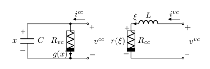
Describing negative resistors in terms of dissipation inequalities opens the way to the use of dissipativity theory to characterize circuit interconnections. As an illustration, consider the parallel interconnection of a voltage-controlled negative resistance element with a capacitor (Figure 3, left). Let and be the currents and voltages associated to the capacitor and the controlled resistor, respectively. The capacitor is a classical lossless element that satisfies the power-preserving equality
| (6) |
In the language of dissipativity theory, the quantity on the left-hand side is the time-derivative of the storage . The negative resistance element satisfies . The parallel interconnection defined by and 11 1 The superindices in the variables and indicate that the port under consideration is current-driven. In a similar way, and will denote the variables associated to a voltage-driven port. satisfies the dissipation (in)equality
| (7) |
The quantity that appears on the left hand-side is the time-derivative of a negative storage. More generally, the storage functions in this paper will be quadratic forms defined by a symmetric matrix with negative eigenvalues (and positive eigenvalues). Such signed storage functions generalize the conventional positive definite storages of passivity theory. Positive definite storages are natural candidates for the stability analysis of closed equilibrium systems. In its incremental form, stability analysis appears in the literature under different names, including contraction theory [24], incremental stability analysis [2], or differential Lyapunov analysis [13]. Signed storages generalize this stability analysis for non-equilibrium behaviors characterized by a low-dimensional asymptotic behavior. This generalization is the topic of dominance analysis, reviewed in the next section.
3 Differential dissipativity
3.1 Dominant systems
Dominance theory extends stability analysis to non-equilibrium behaviors. The approach is based on the intuitive idea that the long run behavior of the system is dictated by low-dimensional dynamics, identified through the study of the system linearization [13], [14], [15]. In what follows we adapt the differential approach of [15] into an incremental setting.
Definition 1.
Let be a Lipschitz continuous map. A system of the form
| (8) |
is -dominant with rate if there exists a matrix with inertia such that
| (9) |
The property is strict if .
When is positive definite, (9) becomes the incremental analogue of the classical Lyapunov inequality, meaning that any two trajectories converge to each other with decay rate at least , [4]. When is a differentiable map, (9) reduces to the simple matrix inequality
| (10) |
Theorem 2.
PROOF.
First assume that (8) is -dominant. Expanding the left-hand side of (9) and dividing by yields,
By letting we arrive to (10). For the converse statement, let and let be such that
where . Hence,
The above inequality implies that is a non-increasing function. Therefore, and (9) follows. This concludes the proof.
The property of dominance strongly constrains the asymptotic behavior of the system as described for the following theorem.
Theorem 3 ([15, Theorem 2]).
Additionally, the following corollary becomes useful in characterizing the asymptotic behavior of a dominant system.
Corollary 4.
Summing up, closed dynamic systems with smaller degrees of dominance will show simpler behaviors compared with systems with higher degrees. The following subsection extends the property of dominance to open systems under the framework of dissipative systems.
3.2 Signed dissipation inequalities
Dissipativity theory [35], [36] is grounded in dissipation inequalities, which generalize the physical characterization of a passive circuit as a system that can only absorb energy: the variation of energy stored in the elements of the circuit (capacitors and inductors) is upper bounded by the electrical power supplied to the circuit. For a linear circuit, the storage is a quadratic function of the state, and the dissipation inequality takes the standard form
The scalar determines a dissipation rate. Each pair of voltage and current appearing in the voltage vector and voltage current determines a port of the circuit.
In matrix form, the quadratic dissipation inequality characterizing passivity reads
| (11) |
An incremental dissipation inequality is in term of the increments rather than absolute variables:
| (12) |
Motivated by the signed supply rates and signed storages introduced in Section 2, we generalize the incremental passivity dissipation inequality (12) to signed dissipation inequalities of the form
| (13) |
for an arbitrary circuit with state and ports defining the current and voltage . We only consider circuits composed of linear capacitors, linear inductors, and nonlinear resistors. The signed quadratic storage is determined by the symmetric matrix with negative eigenvalues and positive eigenvalues. The signed supply is determined by the signature matrix . The scalar is the dissipation rate. The matrices are symmetric as in (3).
Definition 5.
A nonlinear circuit is called signed passive if the inequality (13) holds along any pair of trajectories. The property is strict if .
Definition 5 is very close to the classical definition of incremental passivity. The only difference is that (i) we consider signed storages, i.e. differences of positive storages and (ii) signed supply rates, i.e. differences of the classical passivity supply rates. As illustrated in Section 2, such storages and supply rates appear naturally when considering circuits with both passive and active elements and ports that can both absorb and deliver energy.
3.3 Dissipative interconnections
The central property of passivity theory is that passivity is preserved by interconnection. More precisely, port interconnections of passive circuits are passive. In order to generalize this property to signed-passivity, we introduce the following definition.
Definition 6.
Let and be signed-passive with a common rate . Their interconnection is called dissipative if
| (14) |
If equality holds in (14), then the interconnection is called neutral.
The conventional passivity supply assumes . In this case, an interconnection is neutral if
Hence, port interconnections of passive circuits are neutral. More generally, let us consider the port interconnection of two signed-passive systems as
| (15) |
where we have set and . Here the pairs and are associated to current-controlled and voltage-controlled ports, respectively, see Figures 3 and 4. Substitution of (15) on the left-hand side of (14) shows that port interconnections of signed-passive systems with supplies sharing the same signature (i.e., ) are neutral. Note that a circuit is closed or terminated whenever and .
The question of how to realize a neutral or dissipative interconnection when interconnecting signed-passive circuits is deferred to Section 5. But the definition allows for the following generalization of the passivity theorem.
Theorem 7.
The dissipative interconnection of two signed-passive systems with a common dissipation rate is signed-passive with the same rate. The storage of the interconnected system is the sum of the storages.
PROOF.
Let us consider the aggregated state , and the block-diagonal matrix . The sum of storages satisfies,
| (16) |
A key consequence of the passivity theorem is the property that when a passive system is terminated, it leads to a stable equilibrium system. The storage becomes a Lyapunov function for the closed system. The generalization of that result is as follows.
Theorem 8.
Let be a strictly signed-passive circuit with rate and dominance degree . The terminated circuit built from the dissipative interconnection of with a resistor () defines a -dominant system with the same rate provided that and .
4 Elementary switching and oscillating circuits
In this section we review classical elementary circuits and illustrate their signed passivity properties.
4.1 Switching circuits
We start with the parallel nonlinear circuit and the series nonlinear circuit shown in Figure 3. For the nonlinear circuit, we rewrite the dissipation inequality (7) in the matrix form with state
| (18) |
The dissipation inequality involves the standard storage of a capacitor and the standard supply of a one port circuit, but both with a negative signature.
The circuit is the port interconnection of a capacitor with a negative resistor. The interconnection is neutral as a port interconnection of elements with negative signature . Terminating the circuit, that is, setting , results in a -dominant system when . This closed circuit has one or three equilibria. With three equilibria, one of which unstable, the circuit is an elementary example of bistable switch.
The dissipativity analysis of the series circuit in Figure 3 is similar. Taking as state variable , the circuit satisfies the dissipation inequality
| (19) |
The circuit is a bistable switch when . Both circuits can be seen as abstract realizations of the classical Schmitt trigger circuit in which the negative resistor is usually made by using an operational amplifier in positive feedback [25].
4.2 Oscillating circuits
We proceed with the analysis of the nonlinear RLC circuits shown in Figure 4.

The parallel nonlinear circuit is the port interconnection of the nonlinear circuit in the previous section with a lossless inductor. The port interconnection is neutral as an interconnection of two circuits with supply signature . The total storage is the sum of two negative storages
Defining the state and
the interconnection satisfies the dissipation inequality
| (20) |
The storage has a dominance degree 2 and the supply has a negative signature . When terminated, that is, when , the circuit is 2-dominant for . It is a prototype of negative resistance nonlinear oscillator, such as the circuits studied by Van der Pol [32] and Nagumo [26].
The series interconnection in Figure 4 can be studied in a similar way, as a neutral interconnection between the nonlinear circuit in the previous section and a lossless capacitor. The circuit is signed dissipative with the same storage and with the supply
5 Dissipative interconnections
We return to question of realizing dissipative interconnections satisfying (14). We illustrate the construction with the static coupling network shown in Figure 5.

The interconnection equations are
| (21) |
where the variables , , and , , represent the range of possible ports available after interconnection. With this notation, a port is closed or terminated when and , which is the case shown in Figure 5.
The following theorem provides conditions on the coupling network guaranteeing a dissipative interconnection.
Theorem 9.
The interconnection between and is dissipative if and only if the coupling network is signed-passive without any shortage of signed-passivity, i.e., if and only if satisfies,
| (22) |
with , for all . In addition, the interconnection is neutral if and only if,
| (23) |
PROOF.
The addition of the network adds signed dissipation to both systems, allowing the following generalization of Theorem 8.
Corollary 10.
Let be a strictly signed-passive circuit with rate and dominance degree . The terminated circuit built from dissipative interconnection of with a resistor () through a coupling defines a -dominant system with the same rate provided that
| (25) |
PROOF.
Figures 6-7 illustrate practical realizations of dissipative interconnections where resistive elements model power losses.

The “T” connection in Figure 6 imposes the constraints
where . Without loss of generality we assume that and . It follows from direct computations that the “T” bridge satisfies (22) with
Hence, according to Theorem 9, the interconnection of and via the “T” bridge is dissipative for the case and whenever .

In this case the connection imposes the relations
where . Hence direct computations show that the “” bridge also satisfies (22) with
Following again Theorem 9, the “” bridge provides an interconnection that is dissipative whenever .
Both dissipative interconnections above can be implemented by using negative resistance devices as shown in Figure 8. One should stress that the implementations in Figure 8 only consider the active range of the controlled resistors and .


6 An example

We conclude this paper with an analysis of the circuit shown in Figure 9. The circuits and are the negative resistance switches analyzed in Section 4. From (18)-(19) it becomes clear that their interconnection (denoted as ) is neutral. In addition, Theorem 7 reveals that the resulting circuit is signed-passive with a negative storage (of dominance degree 2) and a passivity supply with negative signature , for all , where and are the positive slopes of the voltage-current characteristics of and respectively.
The circuit is a classical linear passive load. It has a positive definite storage and is passive, that is signed-passive with positive signature supply , for .
The two circuits are interconnected through the “” bridge discussed in the previous section. This element makes the interconnection of and dissipative. As a consequence, the interconnected circuit is signed-passive. Its storage is the difference of two positive definite storages. It has a dominance degree 2. The supply of the interconnected system is a passivity supply with positive signature . The terminated circuit is 2 dominant for any rate satisfying
The simulation in Figure 10 is for the set of parameters , , , , , and . The active resistors , and have voltage-current characteristics given by
Note that the active resistor has an active region with negative slope of and satisfies , thus providing a dissipative coupling locally. Also, with these set of parameters the circuit has a unique unstable equilibrium. The simulated behavior is bounded and entirely in the active range of the controlled resistors. By 2-dominance of the circuit, the trajectory must converge to a limit cycle.
References
- [1] B. D. O. Anderson and S. Vongpanitlerd. Network Analysis and Synthesis: A modern systems theory approach. Dover Publications, 2006.
- [2] D. Angeli. A Lyapunov approach to incremental stability properties. IEEE Transactions on Automatic Control, 47(3):410–421, 2002.
- [3] H. H. Bauschke and P. L. Combettes. Convex Analysis and Monotone Operator Theory in Hilbert Spaces. CMS Books in Mathematics. Springer New York, 2011.
- [4] S. Boyd, L.E. Ghaoui, E. Feron, and V. Balakrishnan. Linear Matrix Inequalities in System and Control Theory. Studies in Applied Mathematics. SIAM, 1994.
- [5] R. K. Brayton and J. K. Moser. A theory of nonlinear networks. I. Quarterly of Applied Mathematics, 22(1):1–33, 1964.
- [6] B. Brogliato, R Lozano, B. Maschke, and O. Egeland. Dissipative Systems Analysis and Control: Theory and Applications. Communications and Control Engineering. Springer Verlag London, 2nd edition, 2007.
- [7] M. K. Camlibel, W. P. M. H. Heemels, and J. M. Schumacher. On linear passive complementarity systems. European Journal of Control, 8(3):220–237, 2002.
- [8] S.-L. Chen, P. B. Griffin, and J. D. Plummer. Negative differential resistance circuit design and memory applications. IEEE Transactions on Electron Devices, 56(4):634–640, 2009.
- [9] L. O. Chua. Dynamic nonlinear networks: state-of-the-art. IEEE Transactions on Circuits and Systems, 27(11):1059–1087, 1980.
- [10] L. O. Chua, C. A. Desoer, and E. S. Kuh. Linear and nonlinear circuits. Mc-Graw Hill, 1987.
- [11] L. O. Chua, J. Yu, and Y. Yu. Negative resistance devices. Circuit Theory and Applications, 11:161–186, 1983.
- [12] C. A. Desoer and M. Vidyasagar. Feedback Systems: Input–Output Properties. Society for Industrial and Applied Mathematics, 2009.
- [13] F. Forni and R. Sepulchre. A differential Lyapunov framework for contraction analysis. IEEE Transactions on Automatic Control, 59(3):614–628, 2014.
- [14] F. Forni and R. Sepulchre. A dissipativity theorem for -dominant systems. In Decision and Control, 56th IEEE Conference on, Melbourne, Australia, December 2017.
- [15] F. Forni and R. Sepulchre. Differential dissipativity theory for dominance analysis. IEEE Transactions on Automatic Control, 2018. in press.
- [16] F. Forni, R. Sepulchre, and A. J. van der Schaft. On differential passivity of physical systems. In Decision and Control, 52rd IEEE Conference on, pages 6580–6585, Florence, Italy, Dec 2013.
- [17] E. Goto, K. Murata, K. Nakazawa, K. Nakagawa, T. Moto-Oka, Y. Matsuoka, Y. Ishibashi, H. Ishida, T. Soma, and E. Wada. Esaki diode high speed logical circuits. IRE Transactions on electronic computers, EC-9(1):25–29, 1960.
- [18] D. J. Hill and P. J. Moylan. Dissipative dynamical systems: basic input-output and state properties. Journal of the Franklin Institute, 309(5):327–357, 1980.
- [19] C.-L. J. Hu. Self-sustained oscillation in an or circuit containing a hysteresis resistor . IEEE Transactions on Circuits and Systems, CAS-33(6):636–641, 1986.
- [20] R. M. Kaplan. Equivalent circuits for negative resistance devices. Technical report, Rome Air Development Center, Griffiss Air Force Base NY, 1968.
- [21] M. P. Kennedy. Three steps to chaos - Part I: Evolution. IEEE Transactions on Circuits and Systems - I, 40(10):640–656, 1993.
- [22] M. P. Kennedy and L. O. Chua. Hysteresis in electronic circuits: a circuit theorist’s perspective. International Journal of Circuit Theory and Applications, 19:471–515, 1991.
- [23] D. Li and Y. Tsividis. Active filters on silicon. In IEE Proceedings - Circuits, Devices and Systems, volume 147, pages 49–56, 2000.
- [24] W. Lohmiller and J-J. E. Slotine. On contraction analysis for nonlinear systems. Automatica, 34(6):683–696, 1998.
- [25] F. A. Miranda-Villatoro, F. Forni, and R. Sepulchre. Dominance analysis of linear complementarity systems. In 23rd International Symposium on Mathematical Theory of Networks and Systems, pages 422–428, Hong Kong, July 2018.
- [26] J. Nagumo, S. Arimoto, and S. Yoshizawa. An active pulse transmission line simulating a nerve axon. Proceedings of the IRE, 50(10):2061–2070, 1962.
- [27] R. Ortega, A. Loría, P. J. Nicklasoon, and H. Sira-Ramírez. Passivity-based Control of Euler-Lagrange Systems: Mechanical, Electrical and Electromechanical Applications. Communications and Control Engineering. Springer, 1998.
- [28] A. V. Proskurnikov, F. Zhang, M. Cao, and J. M. A. Scherpen. A general criterion for synchornization of incrementally dissipative nonlinearly coupled agents. In 2015 European Control Conference (ECC), pages 581–586, Linz, Austria, July 2015.
- [29] T. Saito and S. Nakagawa. Chaos from a hysteresis and switched circuit. Philosophical Transactions of the Royal Society of London. Series A: Physical and Engineering Sciences, 353(1701):47–57, 1995.
- [30] R. Sepulchre, M. Jankovic, and P. V. Kokotovic. Constructive Nonlinear Control. Springer-Verlag, London, 1997.
- [31] G. B. Stan and R. Sepulchre. Analysis of interconnected oscillators by dissipativity theory. IEEE Transactions on Automatic Control, 52(2):256–270, 2007.
- [32] B. Van der Pol. On relaxation oscillations. The London, Edinburgh, and Dublin Philosophical Magazine and Journal of Science, 2(11):978–992, 1926.
- [33] A. J. van der Schaft. L2 - Gain and Passivity Techniques in Nonlinear Control. Communications and Control Engineering. Springer London, second edition, 2010.
- [34] A. J. van der Schaft. On differential passivity. In 9th Symposium on Nonlinear Control Systems, pages 21–25, Toulouse, France, September 2013.
- [35] J. C. Willems. Dissipative dynamical systems part I: General theory. Archive for rational mechanics and analysis, 45(5):321–351, 1972.
- [36] J. C. Willems. Dissipative dynamical systems part II: Linear systems with quadratic supply rates. Archive for rational mechanics and analysis, 45(5):352–393, 1972.