跳到论文正文
W Papers独立论文阅读器 arXiv:1908.11187 论文正文 计算阅读时间 · 0%
引用这篇论文根据当前论文元数据生成,正式投稿前建议核对。


License: arXiv.org perpetual non-exclusive license
arXiv:1908.11187v2 [math.PR] 29 May 2020

Long Range Dependence for Stable Random Processes

Vitalii Makogin Affiliation: Ulm University, E-mails: vitalii.makogin@uni-ulm.de, albert.rapp@uni-ulm.de, evgeny.spodarev@uni-ulm.de    Marco Oesting Affiliation: University of Siegen, E-Mail: oesting@mathematik.uni-siegen.de    Albert Rapp Affiliation: Ulm University, E-mails: vitalii.makogin@uni-ulm.de, albert.rapp@uni-ulm.de, evgeny.spodarev@uni-ulm.de    Evgeny Spodarev Affiliation: Ulm University, E-mails: vitalii.makogin@uni-ulm.de, albert.rapp@uni-ulm.de, evgeny.spodarev@uni-ulm.de
August 11, 2026
Abstract

We investigate long and short memory in α\alpha-stable moving averages and max-stable processes with α\alpha-Fréchet marginal distributions. As these processes are heavy-tailed, we rely on the notion of long range dependence suggested by Kulik and Spodarev 2019 based on the covariance of excursions. Sufficient conditions for the long and short range dependence of α\alpha-stable moving averages are proven in terms of integrability of the corresponding kernel functions. For max-stable processes, the extremal coefficient function is used to state a necessary and sufficient condition for long range dependence.

AMS Subj. Class.: 60G10, 60G52, 60G70.

1  |  Introduction

The occurrence of long memory in time series has been known for a long time starting from the work of Hurst 1951. Since then, this phenomenon has been observed and studied in applications in various fields including biophysical data (Burnecki 2012), network traffics (Pilipauskaitė and Surgailis 2016), neuroscience (Botcharova et al. 2014), and geosciences (Montillet and Yu 2015), etc. A typical example in financial applications (see e.g. Cheung and Lai 1995 and Panas 2001) is a stationary solution of a autoregressive moving average FARIMA(p,d,qp\mathchar 24891\relax d\mathchar 24891\relax q) process with α−\alpha-stable innovations. In light of the variety of applications, a wide range of statistical models and methods for long range dependent processes has been developed, see, for instance, Avram and Taqqu 1986, Kasahara et al. 1988, Kokoszka and Taqqu 1996 for classical ones, and Magdziarz and Weron 2007 Beran et al. 2012, Jach et al. 2012, Koul and Surgailis 2018 for more recent developments. For a broader overview, we recommend the books of Doukhan et al. 2003, Beran et al. 2013, and Samorodnitsky 2016. These instruments rely on the explicit definition of long range dependence (LRD, for short) of a stationary time series or, more generally, a stationary stochastic process X={X⁡(t),t∈T}X=\{X(t)\mathchar 24891\relax\,t\in T\}. Here and throughout this paper, stationarity is understood in the sense that all finite-dimensional distributions of XX are invariant under translations. There are many definitions of LRD in the literature depending on the class of processes to which XX belongs. For instance, if XX has a finite variance the following definition is classical, cf. (Samorodnitsky 2016, P. 194-195):

Definition 1.1

A stationary stochastic process X={X⁡(t),t∈T}X=\{X(t)\mathchar 24891\relax\,t\in T\} on some domain T⊂ℝT\subset\mathbb{R} with 𝔼⁡[|X⁡(0)|2]<∞\mathbb{E}\big[|X(0)|^{2}\big]<\infty is called long range dependent if

∫T|C⁡(t)|​𝑑t=∞,\displaystyle\int_{T}|C(t)|\,\mathrm{d}t=\infty\mathchar 24891\relax

where C⁡(t)=Cov⁡(X⁡(0),X⁡(t))C(t)=\Cov(X(0)\mathchar 24891\relax X(t)), t∈Tt\in T, is its covariance function. For processes in discrete time, the integral above should be changed to a sum.

Also, XX is antipersistent if ∫T|C⁡(t)|​𝑑t<∞\int_{T}|C(t)|\,\mathrm{d}t<\infty, ∫TC⁡(t)​𝑑t=0\int_{T}C(t)\,\mathrm{d}t=0, and short range dependent, otherwise.

Alternative definitions of long memory rely e.g. on the unboundedness of the spectral density of XX at zero, growth comparisons of partial sums, phase transition in limit theorems for sums or maxima, etc., cf. Heyde and Yang 1997; Dehling and Philipp 2002; Samorodnitsky 2004; Lavancier 2006; Giraitis et al. 2012; Beran et al. 2013; Paulauskas 2016; Samorodnitsky 2016; Jach et al. 2012.

Many of these approaches fail for heavy-tailed stochastic processes whose variance does not exist. Such processes occur, for instance, in modelling of network data, in finance and in insurance (see e.g. Kokoszka and Mikosch 1997 who call the FARIMA(p,d,qp\mathchar 24891\relax d\mathchar 24891\relax q) process with α\alpha-stable innovations long range dependent if d∈(0,1−1/α)d\in(0\mathchar 315\relax 1-1/\alpha) or Embrechts et al. 1997; Resnick 2007). In order to allow for the analysis of long memory behaviour in a broader setting, Kulik and Spodarev 2019 propose to consider the covariance of indicator functions of excursions and introduce

Definition 1.2

A real-valued stationary stochastic process X={X⁡(t),t∈T}X=\{X(t)\mathchar 24891\relax\,t\in T\} where TT is an unbounded subset of ℝ\mathbb{R} is short range dependent (SRD) if

∫T\displaystyle\int_{T} ∫ℝ∫ℝ|Cov(𝟙{X(0)>u},𝟙{X(t)>v})|μ(du)μ(dv)dt<∞\displaystyle\int_{\mathbb{R}}\int_{\mathbb{R}}\Big|\Cov(\mathds{1}\{X(0)>u\}\mathchar 24891\relax\mathds{1}\{X(t)>v\})\Big|\,\mu(\mathrm{d}u)\,\mu(\mathrm{d}v)\,\mathrm{d}t<\infty (1)

for any finite measure μ\mu on ℝ\mathbb{R}. Otherwise, i.e. if there exists a finite measure μ\mu such that the integral in inequality (1) is infinite, XX is long range dependent. For stochastic processes in discrete time, the integral ∫T𝑑t\int_{T}\,\mathrm{d}t should be replaced by the summation ∑t∈T:t≠0\sum_{t\in T:\,t\neq 0}.

One major advantage of this definition is that the above covariance exists in any case due to the boundedness of the indicators. Furthermore, the definition turns out to be useful as it offers the applicability of limit theorems for certain functionals of the process of interest.

In practice, however, the computation of the multiple integral in (1) might prove to be tricky. Therefore, we restrict ourselves here to the wide class of positively associated stochastic processes, including the class of infinitely divisible moving average processes with nonnegative kernels (Bulinski and Shashkin 2007, Chapter 1, Theorem 3.27). This will allow us to eliminate the absolute value in (1).

To introduce the notion of positive association, we need the class ℳ⁡(n)\mathcal{M}(n) of real-valued bounded coordinate-wise nondecreasing Borel functions on ℝn\mathbb{R}^{n}, n∈ℕn\in\mathbb{N}. For a real-valued stochastic process X={X⁡(t),t∈T}X=\{X(t)\mathchar 24891\relax\,t\in T\} and a set I⊂TI\subset T, we denote XI={X⁡(t),t∈I}X_{I}=\{X(t)\mathchar 24891\relax\,t\in I\}.

Definition 1.3

A real-valued stochastic process X={X⁡(t),t∈T}X=\{X(t)\mathchar 24891\relax\,t\in T\} is positively associated if Cov⁡(f⁡(XI),g⁡(XJ))≥0\Cov(f(X_{I})\mathchar 24891\relax g(X_{J}))\geq 0 for any disjoint finite subsets I,J⊂TI\mathchar 24891\relax J\subset T and all functions f∈ℳ⁡(|I|)f\in\mathcal{M}(|I|) and g∈ℳ⁡(|J|)g\in\mathcal{M}(|J|).

By setting I={0}I=\{0\} and J={t}J=\{t\} for t≠0t\neq 0, f(x)=𝟙{x>u}f(x)=\mathds{1}\{x>u\} and g(x)=𝟙{x>v}g(x)=\mathds{1}\{x>v\} for u,v∈ℝu\mathchar 24891\relax v\in\mathbb{R}, we have f∈ℳ⁡(|I|)f\in\mathcal{M}(|I|) and g∈ℳ⁡(|J|)g\in\mathcal{M}(|J|). Consequently, for a positively associated stochastic process XX, it holds Cov(𝟙{X(0)>u},𝟙{X(t)>v})=Cov(f(XI),g(XJ))≥0\Cov(\mathds{1}\{X(0)>u\}\mathchar 24891\relax\mathds{1}\{X(t)>v\})=\Cov(f(X_{I})\mathchar 24891\relax g(X_{J}))\geq 0, i.e. the absolute value in (1) can be omitted.

In this paper, we consider two important subclasses of positively associated stationary processes that satisfy certain stability properties. More precisely, we study α\alpha-stable moving averages and max–stable processes with α\alpha-Fréchet marginals. As these processes are heavy-tailed, the classical definition of LRD (1.1) does not apply. Instead, we check 1.2.

With regard to this endeavor, we first establish a general framework to compute the double integral ∫ℝ∫ℝCov(𝟙{X(0)>u},𝟙{X(t)>v})μ(du)μ(dv)\int_{\mathbb{R}}\int_{\mathbb{R}}\Cov(\mathds{1}\{X(0)>u\}\mathchar 24891\relax\mathds{1}\{X(t)>v\})\,\mu(\mathrm{d}u)\,\mu(\mathrm{d}v) by inverting the univariate characteristic function φ⁡(s)\varphi(s) of X⁡(0)X(0) and the bivariate characteristic function φt​(s1,s2)\varphi_{t}(s_{1}\mathchar 24891\relax s_{2}) of (X⁡(0),X⁡(t))(X(0)\mathchar 24891\relax X(t)). Thus, our 2.4 yields

∫ℝ∫ℝCov(𝟙{X(0)>u},𝟙{X(t)>v})μ(du)μ(dv)\displaystyle\int_{\mathbb{R}}\int_{\mathbb{R}}\Cov(\mathds{1}\{X(0)>u\}\mathchar 24891\relax\mathds{1}\{X(t)>v\})\,\mu(\mathrm{d}u)\,\mu(\mathrm{d}v)
=12​π2​∫ℝ+∫ℝ+1s1​s2​Re​{(φt​(s1,−s2)−φ⁡(s1)​φ​(−s2))​ψ⁡(s1)¯​ψ​(s2)}\displaystyle=\frac{1}{2\pi^{2}}\int_{\mathbb{R}_{+}}\int_{\mathbb{R}_{+}}\frac{1}{s_{1}s_{2}}\text{Re}\bigg\{\big(\varphi_{t}(s_{1}\mathchar 24891\relax-s_{2})-\varphi(s_{1})\varphi(-s_{2})\big)\overline{\psi(s_{1})}\psi(s_{2})\bigg\}
−1s1​s2​Re​{(φt​(s1,s2)−φ⁡(s1)​φ​(s2))​ψ⁡(s1)​ψ​(s2)¯}​d​s1​d​s2\displaystyle\hskip 28.45274pt-\frac{1}{s_{1}s_{2}}\text{Re}\bigg\{\big(\varphi_{t}(s_{1}\mathchar 24891\relax s_{2})-\varphi(s_{1})\varphi(s_{2})\big)\overline{\psi(s_{1})\psi(s_{2})}\bigg\}\,\mathrm{d}s_{1}\,\mathrm{d}s_{2}

where ψ⁡(s)=∫ℝexp⁡{i​s​x}​μ​(𝑑x)\psi(s)=\int_{\mathbb{R}}\exp\{isx\}\,\mu(dx) is the Fourier transform of measure μ\mu.
Integrating this relation with respect to tt will establish short or long range dependence according to 1.2. Subsequently, we will apply this result to get the LRD of symmetric α\alpha-stable (Sα\alphaS) moving averages which are defined as follows.

Definition 1.4 (Samorodnitsky and Taqqu 1994)

Let mm be a measurable function with m∈ℒα​(ℝ)m\in{\mathcal{L}}^{\alpha}(\mathbb{R}), α∈(0,2)\alpha\in(0\mathchar 315\relax 2). Then, a Sα\alphaS moving average process with parameter α∈(0,2)\alpha\in(0\mathchar 315\relax 2) and kernel function mm is a stochastic process X={X⁡(t),t∈ℝ}X=\{X(t)\mathchar 24891\relax\,t\in\mathbb{R}\} defined by

X⁡(t)=∫ℝm⁡(t−x)​Λ​(𝑑x),t∈ℝ,\displaystyle X(t)=\int_{\mathbb{R}}m(t-x)\ \Lambda(dx)\mathchar 24891\relax\quad t\in\mathbb{R}\mathchar 24891\relax (2)

where Λ\Lambda is a Sα\alphaS random measure with Lebesgue control measure.

Here and throughout the paper, we use the notation m∈ℒp​(A)m\in{\mathcal{L}}^{p}(A), p>0p>0, to imply that ∫A|m⁡(x)|p​𝑑x<∞\int_{A}|m(x)|^{p}\,\mathrm{d}x<\infty.

Regarding the SRD/LRD of the process XX given in (2), our main result relies on the notion of α\alpha–spectral covariance ρt=∫ℝ(m⁡(−x)​m​(t−x))α/2​𝑑x\rho_{t}=\int_{\mathbb{R}}(m(-x)m(t-x))^{\alpha/2}\,\mathrm{d}x, t∈ℝt\in\mathbb{R}, where m⁡(x)≥0m(x)\geq 0, x∈ℝx\in\mathbb{R}. The α\alpha–spectral covariance was first introduced by Paulauskas 1976 and its properties were studied in Damarackas and Paulauskas 2014 and Damarackas and Paulauskas 2017. In Paulauskas 2016, it was discussed how the integrability of ρt\rho_{t} can be used for the definition of the memory property. Here, we establish by 3.4 that XX is short range dependent if ρt∈ℒ1​(ℝ)\rho_{t}\in{\mathcal{L}}^{1}(\mathbb{R}) or, equivalently, m∈ℒα/2​(ℝ)m\in{\mathcal{L}}^{\alpha/2}(\mathbb{R}). Also, 3.5 establishes long range dependence if ∫ℝ∫ℝ(mα​(x)∧mα​(t))​𝑑x​𝑑t=∞\int_{\mathbb{R}}\int_{\mathbb{R}}(m^{\alpha}(x)\wedge m^{\alpha}(t))\,\mathrm{d}x\,\mathrm{d}t=\infty where a∧ba\wedge b is the minimum of aa and bb. These results hold also for α\alpha-stable linear time series if integrals are replaced by sums.

To put our results into context, one may refer to other research and discussion on memory properties of α−\alpha-stable processes such as Rachev and Samorodnitsky 2002, Maejima and Yamamoto 2003, Samorodnitsky 2004. Also, we demonstrate how our findings are meaningful in practice by detecting LRD in a real world data set consisting of daily log-returns based on the opening price of the Intel corporation share.

Analogously to α\alpha-stable processes, which have become popular as limits of rescaled sums of stochastic processes, max-stable processes have become a widely used concept in extreme value analysis occurring as limiting models for maxima. Thus, they have found applications in various areas such as meteorology (Coles 1993; Buishand et al. 2008; Davison and Gholamrezaee 2012; Oesting et al. 2017, see e.g.), hydrology Asadi et al. 2015 and finance (Zhang and Smith 2010). Max-stable processes are defined as follows.

Definition 1.5

A real-valued stochastic process X={X⁡(t),t∈T}X=\{X(t)\mathchar 24891\relax\ t\in T\} is called a max-stable process if, for all n∈ℕn\in\mathbb{N}, there exist functions an:T→(0,∞)a_{n}:T\to(0\mathchar 24891\relax\infty) and bn:T→ℝb_{n}:T\to\mathbb{R} such that

{maxi=1n​Xi​(t)−bn​(t)an​(t),t∈T}=d{X⁡(t),t∈T},\left\{\max_{i=1}^{n}\frac{X_{i}(t)-b_{n}(t)}{a_{n}(t)}\mathchar 24891\relax\,t\in T\right\}\stackrel{{\scriptstyle d}}{{=}}\{X(t)\mathchar 24891\relax\,t\in T\}\mathchar 24891\relax

where the processes XiX_{i}, i∈ℕi\in\mathbb{N}, are independent copies of XX, and =d\stackrel{{\scriptstyle d}}{{=}} means equality in distribution. If the index set TT is finite, XX is also called a max-stable vector.

It follows from the univariate extreme value theory that the marginal distributions of a max-stable process are either degenerate or follow a Fréchet, Gumbel or Weibull law. While covariances always exist in the Gumbel and Weibull case and, thus, the classical notion of long-range dependence applies, we will consider the case when XX is a stationary max-stable process with α\alpha-Fréchet marginal distributions, i.e. ℙ⁡(X⁡(t)≤x)=exp⁡(−x−α)\PP(X(t)\leq x)=\exp(-x^{-\alpha}) for all x>0x>0 and some α>0\alpha>0 and all t∈Tt\in T. Here, covariances do not exist if α≤2\alpha\leq 2.

In combination with Definition 1.2, a well-established dependence measure for max–stable stochastic processes allows for an easily tractable condition for short and long memory, respectively. More specifically, we use the pairwise extremal coefficient {θt,t∈ℝ}\{\theta_{t}\mathchar 24891\relax\ t\in\mathbb{R}\} defined via the relation ℙ⁡(X⁡(0)≤x,X⁡(t)≤x)=ℙ⁡(X⁡(0)≤x)θt\PP(X(0)\leq x\mathchar 24891\relax\ X(t)\leq x)=\PP(X(0)\leq x)^{\theta_{t}}, which holds for all x>0x>0, to show that a stationary max-stable process with α\alpha-Fréchet marginal distributions is long range dependent if and only if ∫ℝ(2−θt)​𝑑t=∞\int_{\mathbb{R}}(2-\theta_{t})\,\mathrm{d}t=\infty (cf. 4.3).

To summarize, our paper is structured as follows: Section 2 establishes the framework to invert the bivariate characteristic functions. In Section 3, we make use of this framework to find conditions for long range dependence of symmetric α\alpha-stable moving averages and linear time series, while, in Section 4, we investigate long range dependence of a stationary max-stable process with α\alpha-Fréchet marginals. Finally, we model the daily log-returns of an Intel corporation share by a Sα\alphaS moving average XX and show that XX is LRD in Section 5. For the sake of legibility, some of the proofs have been left out of the main part of this paper. They can be found in the Appendix.

2  |  From Characteristic Function to Covariance of Indicators

In this section, we express the covariance of indicators of excursions of random variables above some levels u,vu\mathchar 24891\relax v through their uni- and bivariate characteristic functions. Notice that for random variables UU and VV it holds that

Cov(𝟙{U>u},𝟙{V>v})=ℙ(U≤u,V≤v)−ℙ(U≤u)ℙ(V≤v).\displaystyle\Cov(\mathds{1}\{U>u\}\mathchar 24891\relax\mathds{1}\{V>v\})=\mathbb{P}(U\leq u\mathchar 24891\relax V\leq v)-\mathbb{P}(U\leq u)\mathbb{P}(V\leq v)\mathchar 314\relax (3)
Theorem 2.1

Suppose UU and VV are identically distributed random variables with marginal characteristic function φU\varphi_{U} and joint characteristic function φU​V\varphi_{UV}. Then, for a finite measure μ\mu with its Fourier transform denoted by ψ:ℝ→ℂ,ψ⁡(s)=∫ℝexp⁡{i​s​x}​μ​(𝑑x)\psi:\mathbb{R}\rightarrow\mathbb{C}\mathchar 24891\relax\psi(s)=\int_{\mathbb{R}}\exp\{isx\}\,\mu(dx) it holds that

∫ℝ∫ℝCov(𝟙{U>u},𝟙{V>v})μ(du)μ(dv)\displaystyle\int_{\mathbb{R}}\int_{\mathbb{R}}\Cov(\mathds{1}\{U>u\}\mathchar 24891\relax\mathds{1}\{V>v\})\,\mu(\mathrm{d}u)\,\mu(\mathrm{d}v)
=14​π2​∫ℝ∫ℝ1s1​s2​(φU​(s1)​φU​(s2)−φU​V​(s1,s2))​ψ⁡(s1)​ψ​(s2)¯​d​s1​d​s2\displaystyle=\frac{1}{4\pi^{2}}\int_{\mathbb{R}}\int_{\mathbb{R}}\frac{1}{s_{1}s_{2}}\Big(\varphi_{U}(s_{1})\varphi_{U}(s_{2})-\varphi_{UV}(s_{1}\mathchar 24891\relax s_{2})\Big)\overline{\psi(s_{1})\psi(s_{2})}\ ds_{1}\,ds_{2}
=12​π2∫ℝ+∫ℝ+[1s1​s2Re{(φU​V(s1,−s2)−φU(s1)φU(−s2))ψ⁡(s1)¯ψ(s2)}\displaystyle=\frac{1}{2\pi^{2}}\int_{\mathbb{R}_{+}}\int_{\mathbb{R}_{+}}\bigg[\frac{1}{s_{1}s_{2}}\text{Re}\bigg\{\big(\varphi_{UV}(s_{1}\mathchar 24891\relax-s_{2})-\varphi_{U}(s_{1})\varphi_{U}(-s_{2})\big)\overline{\psi(s_{1})}\psi(s_{2})\bigg\}
−1s1​s2Re{(φU​V(s1,s2)−φU(s1)φU(s2))ψ⁡(s1)​ψ​(s2)¯}]ds1ds2.\displaystyle\hskip 56.9055pt-\frac{1}{s_{1}s_{2}}\text{Re}\bigg\{\big(\varphi_{UV}(s_{1}\mathchar 24891\relax s_{2})-\varphi_{U}(s_{1})\varphi_{U}(s_{2})\big)\overline{\psi(s_{1})\psi(s_{2})}\bigg\}\bigg]\,\mathrm{d}s_{1}\,\mathrm{d}s_{2}\mathchar 314\relax (4)

Proof: Let U′U^{\prime} and V′V^{\prime} be independent copies of UU and VV. Then

∫ℝ∫ℝCov(𝟙{U>u},𝟙{V>v})μ(du)μ(dv)\displaystyle\int_{\mathbb{R}}\int_{\mathbb{R}}\Cov(\mathds{1}\{U>u\}\mathchar 24891\relax\mathds{1}\{V>v\})\,\mu(\mathrm{d}u)\,\mu(\mathrm{d}v)
=∫ℝ∫ℝ𝔼⁡[𝟙​{U>u,V>v}−𝟙​{U′>u,V′>v}]​μ​(𝑑u)​μ​(𝑑v)\displaystyle=\int_{\mathbb{R}}\int_{\mathbb{R}}\mathbb{E}\big[\mathds{1}\{U>u\mathchar 24891\relax V>v\}-\mathds{1}\{U^{\prime}>u\mathchar 24891\relax V^{\prime}>v\}\big]\,\mu(\mathrm{d}u)\,\mu(\mathrm{d}v)
=lima→∞𝔼∫ℝ∫ℝ[𝟙{U>u>−a,V>v>−a}−𝟙{U′>u>−a,V′>v>−a}]μ(du)μ(dv).\displaystyle=\lim_{a\to\infty}\mathbb{E}\int_{\mathbb{R}}\int_{\mathbb{R}}\big[\mathds{1}\big\{U>u>-a\mathchar 24891\relax V>v>-a\big\}-\mathds{1}\big\{U^{\prime}>u>-a\mathchar 24891\relax V^{\prime}>v>-a\big\}\big]\,\mu(\mathrm{d}u)\,\mu(\mathrm{d}v)\mathchar 314\relax (5)

If we denote the difference of the two indicators by fa​(u,v)f_{a}(u\mathchar 24891\relax v), then by (Schilling 2017, Theorem 19.12)11 1 We thank René Schilling for his idea which simplifies our original proof. we get that the last equality in (5) simplifies to

lima→∞14​π2​𝔼​∫ℝ∫ℝf^a​(s1,s2)​ψ⁡(s1)​ψ​(s2)¯​d​s1​d​s2,\displaystyle\lim_{a\to\infty}\frac{1}{4\pi^{2}}\mathbb{E}\int_{\mathbb{R}}\int_{\mathbb{R}}\widehat{f}_{a}(s_{1}\mathchar 24891\relax s_{2})\overline{\psi(s_{1})\psi(s_{2})}\ ds_{1}\,ds_{2}\mathchar 24891\relax (6)

where f^a​(s1,s2)=∫ℝ∫ℝei⁡(s1​u+s2​v)​fa​(u,v)​𝑑u​𝑑v\widehat{f}_{a}(s_{1}\mathchar 24891\relax s_{2})=\int_{\mathbb{R}}\int_{\mathbb{R}}e^{i(s_{1}u+s_{2}v)}f_{a}(u\mathchar 24891\relax v)\ du\,dv. By A.1 one can interchange the expectation and the integrals in equation (6) and computes

𝔼​f^a​(s1,s2)=1s1​s2​(φU​(s1)​φU​(s2)−φU​V​(s1,s2))\displaystyle\mathbb{E}\widehat{f}_{a}(s_{1}\mathchar 24891\relax s_{2})=\frac{1}{s_{1}s_{2}}\Big(\varphi_{U}(s_{1})\varphi_{U}(s_{2})-\varphi_{UV}(s_{1}\mathchar 24891\relax s_{2})\Big) (7)

which is independent of aa. Thus, equation (6) simplifies to

14​π2​∫ℝ∫ℝ1s1​s2​(φU​(s1)​φU​(s2)−φU​V​(s1,s2))​ψ⁡(s1)​ψ​(s2)¯​d​s1​d​s2.\displaystyle\frac{1}{4\pi^{2}}\int_{\mathbb{R}}\int_{\mathbb{R}}\frac{1}{s_{1}s_{2}}\Big(\varphi_{U}(s_{1})\varphi_{U}(s_{2})-\varphi_{UV}(s_{1}\mathchar 24891\relax s_{2})\Big)\overline{\psi(s_{1})\psi(s_{2})}\ ds_{1}\,ds_{2}\mathchar 314\relax

The second identity in (4) follows from splitting the integrals into the positive and negative half-lines and substituting afterwards. ∎

Corollary 2.2

Under the assumptions of 2.1, suppose that the random vector (U,V)(U\mathchar 24891\relax V) is symmetric. Then relation (4) simplifies to

∫ℝ∫ℝCov(𝟙{U>u},𝟙{V>v})μ(du)μ(dv)\displaystyle\int_{\mathbb{R}}\int_{\mathbb{R}}\Cov(\mathds{1}\{U>u\}\mathchar 24891\relax\mathds{1}\{V>v\})\,\mu(\mathrm{d}u)\,\mu(\mathrm{d}v)
=12​π2∫ℝ+∫ℝ+[1s1​s2(φU​V(s1,−s2)−φU(s1)φU(−s2))Re{ψ⁡(s1)¯ψ(s2)}\displaystyle=\frac{1}{2\pi^{2}}\int_{\mathbb{R}_{+}}\int_{\mathbb{R}_{+}}\bigg[\frac{1}{s_{1}s_{2}}\big(\varphi_{UV}(s_{1}\mathchar 24891\relax-s_{2})-\varphi_{U}(s_{1})\varphi_{U}(-s_{2})\big)\text{Re}\big\{\overline{\psi(s_{1})}\psi(s_{2})\big\}
−1s1​s2(φU​V(s1,s2)−φU(s1)φU(s2))Re{ψ(s1)ψ(s2)}]ds1ds2\displaystyle\hskip 56.9055pt-\frac{1}{s_{1}s_{2}}\big(\varphi_{UV}(s_{1}\mathchar 24891\relax s_{2})-\varphi_{U}(s_{1})\varphi_{U}(s_{2})\big)\text{Re}\big\{\psi(s_{1})\psi(s_{2})\big\}\bigg]\,\mathrm{d}s_{1}\,\mathrm{d}s_{2} (8)
=12​π2​∫ℝ+∫ℝ+1s1​s2​(φU​V​(s1,−s2)−φU​V​(s1,s2))​Re​{ψ⁡(s1)}​Re​{ψ⁡(s2)}\displaystyle=\frac{1}{2\pi^{2}}\int_{\mathbb{R}_{+}}\int_{\mathbb{R}_{+}}\frac{1}{s_{1}s_{2}}\Big(\varphi_{UV}(s_{1}\mathchar 24891\relax-s_{2})-\varphi_{UV}(s_{1}\mathchar 24891\relax s_{2})\Big)\text{Re}\{\psi(s_{1})\}\text{Re}\{\psi(s_{2})\}
+1s1​s2​(φU​V​(s1,−s2)+φU​V​(s1,s2)−2​φU​(s1)​φU​(s2))​Im​{ψ⁡(s1)}​Im​{ψ⁡(s2)}​d​s1​d​s2.\displaystyle\hskip 14.22636pt+\frac{1}{s_{1}s_{2}}\Big(\varphi_{UV}(s_{1}\mathchar 24891\relax-s_{2})+\varphi_{UV}(s_{1}\mathchar 24891\relax s_{2})-2\varphi_{U}(s_{1})\varphi_{U}(s_{2})\Big)\text{Im}\{\psi(s_{1})\}\text{Im}\{\psi(s_{2})\}\,\mathrm{d}s_{1}\,\mathrm{d}s_{2}\mathchar 314\relax (9)
Proof.

Equality (8) follows immediately from φU\varphi_{U} and φU​V\varphi_{UV} being real-valued as characteristic functions of a symmetric random variable and random vector, respectively.

Equality (9) follows from Re​{x​y}=Re​{x}​Re​{y}−Im​{x}​Im​{y}\text{Re}\{xy\}=\text{Re}\{x\}\text{Re}\{y\}-\text{Im}\{x\}\text{Im}\{y\} for any x,y∈ℂx\mathchar 24891\relax y\in\mathbb{C}. ∎

If the stationary real-valued stochastic process X={X⁡(t),t∈ℝ}X=\{X(t)\mathchar 24891\relax t\in\mathbb{R}\} is positively associated, we can apply 2.1 and, in the symmetric case, 2.2 to X⁡(0)X(0) and X⁡(t)X(t) to check the long range dependence of XX.
To do so, let T=ℝT=\mathbb{R} in integral (1). However, the resulting expressions in (4), (8) or (9) might prove difficult to integrate w.r.t. tt over the whole real line. Thus, it is worth noting that the following lemma allows us to restrict integration to unbounded subsets over which it might be easier to integrate.

Lemma 2.3

Let |⋅||\cdot| denote the Lebesgue measure on ℝ\mathbb{R} and let A⊂ℝA\subset\mathbb{R} be an arbitrary subset with |Ac|<∞|A^{c}|<\infty. Then, a process X={X⁡(t),t∈ℝ}X=\{X(t)\mathchar 24891\relax\,t\in\mathbb{R}\} is SRD or LRD iff XA={X⁡(t),t∈A}X_{A}=\{X(t)\mathchar 24891\relax\,t\in A\} is SRD or LRD, respectively.

Proof: We split up the integral in relation (1) into AA and AcA^{c}

∫ℝ∫ℝ∫ℝ|Cov(𝟙{X(0)>u},𝟙{X(t)>v})|μ(du)μ(dv)dt\displaystyle\int_{\mathbb{R}}\int_{\mathbb{R}}\int_{\mathbb{R}}\bigg|\text{Cov}\bigg(\mathds{1}\big\{X(0)>u\big\}\mathchar 24891\relax\mathds{1}\big\{X(t)>v\big\}\bigg)\bigg|\,\mu(\mathrm{d}u)\,\mu(\mathrm{d}v)\,\mathrm{d}t
=\displaystyle= ∫A∫ℝ∫ℝ|Cov(𝟙{X(0)>u},𝟙{X(t)>v})|μ(du)μ(dv)dt\displaystyle\int_{A}\int_{\mathbb{R}}\int_{\mathbb{R}}\bigg|\text{Cov}\bigg(\mathds{1}\big\{X(0)>u\big\}\mathchar 24891\relax\mathds{1}\big\{X(t)>v\big\}\bigg)\bigg|\,\mu(\mathrm{d}u)\,\mu(\mathrm{d}v)\,\mathrm{d}t
+∫Ac∫ℝ∫ℝ|Cov(𝟙{X(0)>u},𝟙{X(t)>v})|⏟≤1μ(du)μ(dv)dt.\displaystyle+\int_{A^{c}}\int_{\mathbb{R}}\int_{\mathbb{R}}\underbrace{\bigg|\text{Cov}\bigg(\mathds{1}\big\{X(0)>u\big\}\mathchar 24891\relax\mathds{1}\big\{X(t)>v\big\}\bigg)\bigg|}_{\leq 1}\,\mu(\mathrm{d}u)\,\mu(\mathrm{d}v)\,\mathrm{d}t\mathchar 314\relax

As the integral over AcA^{c} is finite in any case, the integral in relation (1) is finite iff XAX_{A} is SRD. ∎

Now we give the main result of this section showing the use of characteristic functions to check the short or long range dependence of XX.

Theorem 2.4

Suppose we have a stationary real-valued, positively associated stochastic process X={X⁡(t),t∈ℝ}X=\{X(t)\mathchar 24891\relax\,t\in\mathbb{R}\} with absolutely continuous marginal distributions. Denote the univariate characteristic function of X⁡(0)X(0) by φ\varphi and the bivariate characteristic function of (X⁡(0),X⁡(t))(X(0)\mathchar 24891\relax X(t)) by φt\varphi_{t}. Furthermore, let A⊂ℝA\subset\mathbb{R} be an arbitrary subset with |Ac|<∞|A^{c}|<\infty.

  1. (a)

    Then, XX is short range dependent if

    ∫A\displaystyle\int_{A} ∫ℝ∫ℝCov(𝟙{X(0)>u},𝟙{X(t)>v})μ(du)μ(dv)dt\displaystyle\int_{\mathbb{R}}\int_{\mathbb{R}}\Cov(\mathds{1}\{X(0)>u\}\mathchar 24891\relax\mathds{1}\{X(t)>v\})\,\mu(\mathrm{d}u)\,\mu(\mathrm{d}v)\,\mathrm{d}t
    =12​π2∫A∫ℝ+∫ℝ+[1s1​s2Re{(φt(s1,−s2)−φ(s1)φ(−s2))ψ⁡(s1)¯ψ(s2)}\displaystyle=\frac{1}{2\pi^{2}}\int_{A}\int_{\mathbb{R}_{+}}\int_{\mathbb{R}_{+}}\bigg[\frac{1}{s_{1}s_{2}}\text{Re}\bigg\{\big(\varphi_{t}(s_{1}\mathchar 24891\relax-s_{2})-\varphi(s_{1})\varphi(-s_{2})\big)\overline{\psi(s_{1})}\psi(s_{2})\bigg\}
    −1s1​s2Re{(φt(s1,s2)−φ(s1)φ(s2))ψ⁡(s1)​ψ​(s2)¯}]ds1ds2dt<∞\displaystyle\hskip 28.45274pt-\frac{1}{s_{1}s_{2}}\text{Re}\bigg\{\big(\varphi_{t}(s_{1}\mathchar 24891\relax s_{2})-\varphi(s_{1})\varphi(s_{2})\big)\overline{\psi(s_{1})\psi(s_{2})}\bigg\}\bigg]\,\mathrm{d}s_{1}\,\mathrm{d}s_{2}\,\mathrm{d}t<\infty (10)

    for any finite measure μ\mu with Fourier transform ψ⁡(s)=∫ℝexp⁡{i​s​x}​μ​(𝑑x)\psi(s)=\int_{\mathbb{R}}\exp\{isx\}\,\mu(dx).

  2. (b)

    Additionally, if (X⁡(0),X⁡(t))(X(0)\mathchar 24891\relax X(t)) is symmetric for all t∈ℝt\in\mathbb{R}, then condition (10) rewrites as

    ∫A∫ℝ∫ℝCov(𝟙{X(0)>u},𝟙{X(t)>v})μ(du)μ(dv)dt\displaystyle\int_{A}\int_{\mathbb{R}}\int_{\mathbb{R}}\Cov(\mathds{1}\{X(0)>u\}\mathchar 24891\relax\mathds{1}\{X(t)>v\})\,\mu(\mathrm{d}u)\,\mu(\mathrm{d}v)\,\mathrm{d}t
    =12​π2∫A∫ℝ+∫ℝ+[φt​(s1,−s2)−φt​(s1,s2)s1​s2Re{ψ(s1)}Re{ψ(s2)}\displaystyle=\frac{1}{2\pi^{2}}\int_{A}\int_{\mathbb{R}_{+}}\int_{\mathbb{R}_{+}}\bigg[\frac{\varphi_{t}(s_{1}\mathchar 24891\relax-s_{2})-\varphi_{t}(s_{1}\mathchar 24891\relax s_{2})}{s_{1}s_{2}}\text{Re}\{\psi(s_{1})\}\text{Re}\{\psi(s_{2})\}
    −φt​(s1,−s2)+φt​(s1,s2)−2​φ​(s1)​φ​(s2)s1​s2Im{ψ(s1)}Im{ψ(s2)}]ds1ds2dt<∞.\displaystyle-\frac{\varphi_{t}(s_{1}\mathchar 24891\relax-s_{2})+\varphi_{t}(s_{1}\mathchar 24891\relax s_{2})-2\varphi(s_{1})\varphi(s_{2})}{s_{1}s_{2}}\text{Im}\{\psi(s_{1})\}\text{Im}\{\psi(s_{2})\}\bigg]\,\mathrm{d}s_{1}\,\mathrm{d}s_{2}\,\mathrm{d}t<\infty\mathchar 314\relax (11)

Otherwise, i.e. if there exists a finite measure μ\mu such that the integral in (10) is infinite, XX is long range dependent.

Proof:

  1. (a)

    Take U=X⁡(0)U=X(0) and V=X⁡(t),V=X(t)\mathchar 24891\relax where t∈ℝt\in\mathbb{R} in 2.1. Then, UU and VV are absolutely continuous and identically distributed random variables. Therefore, the equality in (10) is established by 2.1. It follows by relation (10) and 2.3 that XX is SRD. Similarly, XX is LRD if (10) is infinite.

  2. (b)

    Follows analogously by using 2.2.

∎

3  |  Long Range Dependence of α\alpha–stable Moving Averages

In this section, we investigate the LRD of Sα\alphaS moving averages in continuous and discrete time.

By 1.4, a symmetric α\alpha-stable moving average with kernel function m∈ℒα​(ℝ)m\in{\mathcal{L}}^{\alpha}(\mathbb{R}), α<2\alpha<2, is defined by X⁡(t)=∫ℝm⁡(t−x)​Λ​(𝑑x)X(t)=\int_{\mathbb{R}}m(t-x)\ \Lambda(\mathrm{d}x), t∈ℝt\in\mathbb{R}, where Λ\Lambda is a symmetric α\alpha-stable random measure.

Remark 3.1
  1. (a)

    Note that the Sα\alphaS moving average process X={X⁡(t),t∈ℝ}X=\{X(t)\mathchar 24891\relax\,t\in\mathbb{R}\} is stationary, X⁡(0)X(0) is absolutely continuous and, by Property 3.2.1 from Samorodnitsky and Taqqu 1994, the random vector (X⁡(0),X⁡(t))(X(0)\mathchar 24891\relax X(t)) is symmetric for every t∈ℝt\in\mathbb{R}.

  2. (b)

    By Bulinski and Shashkin 2007, Theorems 1.3.5 and 1.3.27, XX is positively associated if the kernel function mm is nonnegative.

  3. (c)

    To exclude the trivial case X⁡(t)=0X(t)=0 for all t∈ℝt\in\mathbb{R} we always assume that the Lebesgue measure of the set {x∈ℝ|m⁡(x)>0}\{x\in\mathbb{R}\,|\;m(x)>0\} is positive.

By Samorodnitsky and Taqqu 1994, Proposition 3.4.2., the characteristic function φ:ℝ→ℂ\varphi:\mathbb{R}\to\mathbb{C} of X⁡(t)X(t), t∈ℝt\in\mathbb{R}, is given by

φ(s)=exp{−|s|α∫ℝ|m(x)|αdx},s∈ℝ.\displaystyle\varphi(s)=\exp\bigg\{-|s|^{\alpha}\int_{\mathbb{R}}|m(x)|^{\alpha}\,\mathrm{d}x\bigg\}\mathchar 24891\relax\quad s\in\mathbb{R}\mathchar 314\relax (12)

Moreover, the bivariate characteristic function φt:ℝ×ℝ→ℂ\varphi_{t}:\mathbb{R}\times\mathbb{R}\to\mathbb{C} of (X⁡(0),X⁡(t)),\big(X(0)\mathchar 24891\relax X(t)\big)\mathchar 24891\relax t∈ℝt\in\mathbb{R} is given by

φt(s1,s2)=exp{−∫ℝ|s1m(−x)+s2m(t−x)|αdx},s1,s2∈ℝ.\displaystyle\varphi_{t}(s_{1}\mathchar 24891\relax s_{2})=\exp\bigg\{-\int_{\mathbb{R}}|s_{1}m(-x)+s_{2}m(t-x)|^{\alpha}\,\mathrm{d}x\bigg\}\mathchar 24891\relax\quad s_{1}\mathchar 24891\relax s_{2}\in\mathbb{R}\mathchar 314\relax (13)

Before we get to our main result, we need to introduce the α\alpha-spectral covariance of a stable vector as defined by (Damarackas and Paulauskas 2017, equation (11)). Let 𝕊1={𝐱∈ℝ2:‖𝐱‖=1}\mathbb{S}^{1}=\{\mathbf{x}\in\mathbb{R}^{2}:\|\mathbf{x}\|=1\} be the unit circle. Recall that a random vector Z=(X1,X2)Z=(X_{1}\mathchar 24891\relax X_{2}) is symmetric α\alpha-stable with parameter α\alpha if there exists a finite measure Γ\Gamma on 𝕊1\mathbb{S}^{1}, the so-called spectral measure, such that the characteristic function of ZZ is given by

𝔼ei​⟨s,Z⟩=exp{−∫𝕊1|⟨s,x⟩|αΓ(dx)},s∈ℝ2,\displaystyle\mathbb{E}e^{i\langle s\mathchar 24891\relax Z\rangle}=\exp\bigg\{-\int_{\mathbb{S}^{1}}|\langle s\mathchar 24891\relax x\rangle|^{\alpha}\Gamma(dx)\bigg\}\mathchar 24891\relax s\in\mathbb{R}^{2}\mathchar 24891\relax

where ⟨⋅,⋅⟩\langle\cdot\,\mathchar 24891\relax\cdot\rangle is the standard inner product on ℝ2\mathbb{R}^{2}.

Definition 3.2

Suppose (X1,X2)(X_{1}\mathchar 24891\relax X_{2}) is an α\alpha-stable random vector with spectral measure Γ\Gamma, then the α\alpha-spectral covariance of X1X_{1} and X2X_{2} is given by

ρ=∫𝕊1|s1​s2|α/2​sgn⁡(s1​s2)​Γ​(d⁡(s1,s2)).\displaystyle\rho=\int_{\mathbb{S}^{1}}|s_{1}s_{2}|^{\alpha/2}\sgn(s_{1}s_{2})\ \Gamma(d(s_{1}\mathchar 24891\relax s_{2}))\mathchar 314\relax (14)

Let us calculate the α\alpha-spectral covariance of (X⁡(0),X⁡(t))(X(0)\mathchar 24891\relax X(t)), t∈ℝt\in\mathbb{R}, where XX is a Sα\alphaS moving average.

Lemma 3.3

Suppose X={X⁡(t),t∈ℝ}X=\{X(t)\mathchar 24891\relax t\in\mathbb{R}\} with X⁡(t)=∫ℝm⁡(t−x)​Λ​(𝑑x)X(t)=\int_{\mathbb{R}}m(t-x)\ \Lambda(dx) is a Sα\alphaS moving average process. Then, the α\alpha-spectral covariance of (X⁡(0),X⁡(t))(X(0)\mathchar 24891\relax X(t)), t∈ℝt\in\mathbb{R}, is given by

ρt=∫ℝmα/2​(−x)​mα/2​(t−x)​sgn⁡(m⁡(−x)​m​(t−x))​𝑑x.\displaystyle\rho_{t}=\int_{\mathbb{R}}m^{\alpha/2}(-x)m^{\alpha/2}(t-x)\sgn(m(-x)m(t-x))\,\mathrm{d}x\mathchar 314\relax (15)

Proof: Denote m1​(x)=m​(−x)m_{1}(x)=m(-x) and m2​(x)=m⁡(t−x)m_{2}(x)=m(t-x), Proposition 3.4.3 in Samorodnitsky and Taqqu 1994 and the the symmetry of Λ\Lambda yields that (X⁡(0),X⁡(t))(X(0)\mathchar 24891\relax X(t)) is Sα\alphaS with spectral measure Γ\Gamma defined for all Borel sets A⊂𝕊1A\subset\mathbb{S}^{1} by

Γ⁡(A)\displaystyle\Gamma(A) =12​∫g−1​(A)(m12​(x)+m22​(x))α/2​𝑑x+12​∫g−1​(−A)(m12​(x)+m22​(x))α/2​𝑑x\displaystyle=\frac{1}{2}\int_{g^{-1}(A)}\Big(m_{1}^{2}(x)+m_{2}^{2}(x)\Big)^{\alpha/2}\,\mathrm{d}x+\frac{1}{2}\int_{g^{-1}(-A)}\Big(m_{1}^{2}(x)+m_{2}^{2}(x)\Big)^{\alpha/2}\,\mathrm{d}x
=γ⁡(g−1​(A))+γ⁡(g−1​(−A))=:(γ∘g−1)​(A)+(γ∘g−1)​(−A),\displaystyle=\gamma(g^{-1}(A))+\gamma(g^{-1}(-A))=:(\gamma\circ g^{-1})(A)+(\gamma\circ g^{-1})(-A)\mathchar 24891\relax

where

g⁡(x)=(m1​(x)(m12​(x)+m22​(x))1/2,m2​(x)(m12​(x)+m22​(x))1/2),x∈ℝ.\displaystyle g(x)=\left(\frac{m_{1}(x)}{\big(m_{1}^{2}(x)+m_{2}^{2}(x)\big)^{1/2}}\ \mathchar 24891\relax\ \frac{m_{2}(x)}{\big(m_{1}^{2}(x)+m_{2}^{2}(x)\big)^{1/2}}\right)\mathchar 24891\relax\quad x\in\mathbb{R}\mathchar 314\relax

Hereby γ\gamma is an absolutely continuous measure w.r.t. the Lebesgue measure with density 12​(m12​(x)+m22​(x))α/2\frac{1}{2}(m_{1}^{2}(x)+m_{2}^{2}(x))^{\alpha/2}. With f⁡(s1,s2)=|s1​s2|α/2​sgn⁡(s1​s2)f(s_{1}\mathchar 24891\relax s_{2})=|s_{1}s_{2}|^{\alpha/2}\sgn(s_{1}s_{2}) we get

∫𝕊1f​d​(γ∘g−1)\displaystyle\int_{\mathbb{S}^{1}}f\ d(\gamma\circ g^{-1}) =∫g−1​(𝕊1)f∘g​𝑑γ=∫ℝm1α/2​(x)​m2α/2​(x)​sgn⁡(m1​(x)​m2​(x))(m12​(x)+m22​(x))α/2​γ​(𝑑x)\displaystyle=\int_{g^{-1}(\mathbb{S}^{1})}f\circ g\ d\gamma=\int_{\mathbb{R}}\frac{m_{1}^{\alpha/2}(x)\,m_{2}^{\alpha/2}(x)\sgn(m_{1}(x)m_{2}(x))}{\big(m_{1}^{2}(x)+m_{2}^{2}(x)\big)^{\alpha/2}}\,\gamma(dx)
=12​∫ℝm1α/2​(x)​m2α/2​(x)​sgn⁡(m1​(x)​m2​(x))​𝑑x.\displaystyle=\frac{1}{2}\int_{\mathbb{R}}m_{1}^{\alpha/2}(x)\,m_{2}^{\alpha/2}(x)\sgn(m_{1}(x)m_{2}(x))\,\mathrm{d}x\mathchar 314\relax

Thus,

ρt=∫𝕊1|s1​s2|α/2​sgn⁡(s1​s2)​Γ​(d⁡(s1,s2))=∫ℝm1α/2​(x)​m2α/2​(x)​sgn⁡(m1​(x)​m2​(x))​𝑑x.\displaystyle\rho_{t}=\int_{\mathbb{S}^{1}}|s_{1}s_{2}|^{\alpha/2}\sgn(s_{1}s_{2})\ \Gamma(d(s_{1}\mathchar 24891\relax s_{2}))=\int_{\mathbb{R}}m_{1}^{\alpha/2}(x)\,m_{2}^{\alpha/2}(x)\sgn(m_{1}(x)m_{2}(x))\,\mathrm{d}x\mathchar 314\relax

∎

Now, a sufficient condition for the short range dependence of XX can be formulated in terms of ρt\rho_{t} or, equivalently, in terms of the kernel function mm.

Theorem 3.4

Let X={X⁡(t),t∈ℝ}X=\{X(t)\mathchar 24891\relax t\in\mathbb{R}\} be a Sα\alphaS moving average process with parameter α∈(0,2)\alpha\in(0\mathchar 24891\relax 2), nonnegative kernel function mm and α\alpha-spectral covariance ρt\rho_{t} given in (15). XX is SRD if

ρt∈ℒ1​(ℝ),\displaystyle\rho_{t}\in{\mathcal{L}}^{1}(\mathbb{R})\mathchar 24891\relax (16)

or, equivalently, m∈ℒα/2​(ℝ)m\in{\mathcal{L}}^{\alpha/2}(\mathbb{R}).

Proof: Without loss of generality, assume μ\mu is a probability measure. Now, apply 2.4 to XX for some ε∈(0,‖m‖αα)\varepsilon\in(0\mathchar 24891\relax{\|m\|}^{\alpha}_{\alpha}) and choose A={t∈ℝ|ρt∈[0,ε)}.A=\{t\in\mathbb{R}\ |\ \rho_{t}\in[0\mathchar 24891\relax\varepsilon)\}\mathchar 314\relax It follows from the integrability of ρt\rho_{t} that ρt→0\rho_{t}\rightarrow 0 as t→±∞t\rightarrow\pm\infty. Thus, there exists a constant t~>0\tilde{t}>0 such that ρt<ε\rho_{t}<\varepsilon for all t∈ℝt\in\mathbb{R} where |t|>t~|t|>\tilde{t}. Hence, it holds that Ac⊂{t∈ℝ||t|≤t~}A^{c}\subset\big\{t\in\mathbb{R}\ \big|\ |t|\leq\tilde{t}\big\} and |Ac|<∞.|A^{c}|<\infty\mathchar 314\relax

Obviously, the right-hand side of the equality in (11) is bounded by

12​π2​∫A∫ℝ+∫ℝ+|φt​(s1,−s2)−φt​(s1,s2)|s1​s2​|Re​{ψ⁡(s1)}​Re​{ψ⁡(s2)}|⏟≤1​d​s1​d​s2​𝑑t\displaystyle\frac{1}{2\pi^{2}}\int_{A}\int_{\mathbb{R}_{+}}\int_{\mathbb{R}_{+}}\frac{|\varphi_{t}(s_{1}\mathchar 24891\relax-s_{2})-\varphi_{t}(s_{1}\mathchar 24891\relax s_{2})|}{s_{1}s_{2}}\underbrace{\big|\text{Re}\{\psi(s_{1})\}\text{Re}\{\psi(s_{2})\}\big|}_{\leq 1}\mathrm{d}s_{1}\,\mathrm{d}s_{2}\mathrm{d}t
+\displaystyle+ 12​π2​∫A∫ℝ+∫ℝ+|φt​(s1,−s2)+φt​(s1,s2)−2​φ​(s1)​φ​(s2)|s1​s2​|Im​{ψ⁡(s1)}​Im​{ψ⁡(s2)}|⏟≤1​d​s1​d​s2​𝑑t\displaystyle\frac{1}{2\pi^{2}}\int_{A}\int_{\mathbb{R}_{+}}\int_{\mathbb{R}_{+}}\frac{|\varphi_{t}(s_{1}\mathchar 24891\relax-s_{2})+\varphi_{t}(s_{1}\mathchar 24891\relax s_{2})-2\varphi(s_{1})\varphi(s_{2})|}{s_{1}s_{2}}\underbrace{\big|\text{Im}\{\psi(s_{1})\}\text{Im}\{\psi(s_{2})\}\big|}_{\leq 1}\,\mathrm{d}s_{1}\,\mathrm{d}s_{2}\,\mathrm{d}t
≤\displaystyle\leq 1π2​∫A∫ℝ+∫ℝ+|φt​(s1,−s2)−φ⁡(s1)​φ​(s2)|s1​s2​d​s1​d​s2​𝑑t\displaystyle\frac{1}{\pi^{2}}\int_{A}\int_{\mathbb{R}_{+}}\int_{\mathbb{R}_{+}}\frac{|\varphi_{t}(s_{1}\mathchar 24891\relax-s_{2})-\varphi(s_{1})\varphi(s_{2})|}{s_{1}s_{2}}\mathrm{d}s_{1}\,\mathrm{d}s_{2}\mathrm{d}t
+\displaystyle+ 1π2​∫A∫ℝ+∫ℝ+|φt​(s1,s2)−φ⁡(s1)​φ​(s2)|s1​s2​d​s1​d​s2​𝑑t=:1π2​(I1+I2).\displaystyle\frac{1}{\pi^{2}}\int_{A}\int_{\mathbb{R}_{+}}\int_{\mathbb{R}_{+}}\frac{|\varphi_{t}(s_{1}\mathchar 24891\relax s_{2})-\varphi(s_{1})\varphi(s_{2})|}{s_{1}s_{2}}\,\mathrm{d}s_{1}\,\mathrm{d}s_{2}\,\mathrm{d}t=:\frac{1}{\pi^{2}}\left(I_{1}+I_{2}\right)\mathchar 314\relax (17)

By inequalities (32) and (33) in Lemma A.3 we get

I1,I2≤8​πα2​‖m‖α2​α​∫Aρt‖m‖α2​α−ρt2​𝑑t≤8​πα2​‖m‖α2​α​1‖m‖α2​α−ε2​∫Aρt​𝑑t<∞.I_{1}\mathchar 24891\relax I_{2}\leq\frac{8\pi}{\alpha^{2}\|m\|_{\alpha}^{2\alpha}}\int_{A}\frac{\rho_{t}}{\sqrt{\|m\|_{\alpha}^{2\alpha}-\rho_{t}^{2}}}\,\mathrm{d}t\leq\frac{8\pi}{\alpha^{2}\|m\|_{\alpha}^{2\alpha}}\frac{1}{\sqrt{\|m\|_{\alpha}^{2\alpha}-\varepsilon^{2}}}\int_{A}\rho_{t}\,\mathrm{d}t<\infty\mathchar 314\relax

Next, show that condition (16) holds true iff m∈ℒα/2​(ℝ)m\in{\mathcal{L}}^{\alpha/2}(\mathbb{R}). By Fubini’s theorem we get

∫ℝρt​𝑑t\displaystyle\int_{\mathbb{R}}\rho_{t}\,\mathrm{d}t =∫ℝ∫ℝmα/2​(−x)​mα/2​(t−x)​𝑑x​𝑑t\displaystyle=\int_{\mathbb{R}}\int_{\mathbb{R}}m^{\alpha/2}(-x)m^{\alpha/2}(t-x)\,\mathrm{d}x\,\mathrm{d}t
=∫ℝmα/2​(−x)​(∫ℝmα/2​(t−x)​𝑑t)​𝑑x\displaystyle=\int_{\mathbb{R}}m^{\alpha/2}(-x)\bigg(\int_{\mathbb{R}}m^{\alpha/2}(t-x)\,\mathrm{d}t\bigg)\,\mathrm{d}x
=(∫ℝmα/2​(−x)​𝑑x)2=‖m‖α/2α<∞.\displaystyle=\bigg(\int_{\mathbb{R}}m^{\alpha/2}(-x)\,\mathrm{d}x\bigg)^{2}=\|m\|_{\alpha/2}^{\alpha}<\infty\mathchar 314\relax

∎

Naturally, one may also ask for sufficient conditions for the long range dependence of XX. Such a condition is given by

Theorem 3.5

Let X={X⁡(t),t∈ℝ}X=\{X(t)\mathchar 24891\relax t\in\mathbb{R}\} be a Sα\alphaS moving average process with parameter α∈(0,2)\alpha\in(0\mathchar 24891\relax 2) and nonnegative kernel function mm. Then, XX is long range dependent if

∫ℝ∫ℝ(mα​(x)∧mα​(t))​𝑑x​𝑑t=∞.\displaystyle\int_{\mathbb{R}}\int_{\mathbb{R}}(m^{\alpha}(x)\wedge m^{\alpha}(t))\,\mathrm{d}x\,\mathrm{d}t=\infty\mathchar 314\relax (18)

Proof: Given in the appendix. ∎

Additionally, if the kernel function mm is eventually monotonic, then we can simplify condition (18) as follows.

Corollary 3.6

Let X={X⁡(t),t∈ℝ}X=\{X(t)\mathchar 24891\relax t\in\mathbb{R}\} be a Sα\alphaS moving average process with parameter α∈(0,2)\alpha\in(0\mathchar 24891\relax 2) and nonnegative kernel function m∈ℒα​(ℝ)m\in{\mathcal{L}}^{\alpha}(\mathbb{R}) which is eventually monotonic, i.e. there is a number a>0a>0 such that mm is monotonically decreasing on (a,∞)(a\mathchar 24891\relax\infty) or monotonically increasing on (−∞,−a)(-\infty\mathchar 24891\relax-a). Then, XX is long range dependent if

∫a∞t​mα​(t)​𝑑t=∞ or ∫−∞−at​mα​(t)​𝑑t=−∞.\displaystyle\int_{a}^{\infty}t\,m^{\alpha}(t)\,\mathrm{d}t=\infty\quad\text{ or }\quad\int_{-\infty}^{-a}t\,m^{\alpha}(t)\,\mathrm{d}t=-\infty\mathchar 314\relax (19)

Additionally, if mm is symmetric, the two sufficient conditions (19) are equivalent.

Proof.

Suppose mm is monotonically decreasing on (a,∞)(a\mathchar 24891\relax\infty) and compute the integral (18). Thus, we have

∫ℝ∫ℝ(mα​(x)∧mα​(t))​𝑑x​𝑑t≥∫a∞(∫atmα​(t)​𝑑x+∫t∞mα​(x)​𝑑x)​𝑑t≥∫a∞t​mα​(t)​𝑑t−a​‖m‖αα.\displaystyle\int_{\mathbb{R}}\int_{\mathbb{R}}(m^{\alpha}(x)\wedge m^{\alpha}(t))\,\mathrm{d}x\,\mathrm{d}t\geq\int_{a}^{\infty}\bigg(\int_{a}^{t}m^{\alpha}(t)\,\mathrm{d}x+\int_{t}^{\infty}m^{\alpha}(x)\,\mathrm{d}x\bigg)\,\mathrm{d}t\geq\int_{a}^{\infty}tm^{\alpha}(t)\,\mathrm{d}t-a\|m\|^{\alpha}_{\alpha}\mathchar 314\relax

The claim follows from the fact that m∈ℒα​(ℝ)m\in{\mathcal{L}}^{\alpha}(\mathbb{R}). The case of mm monotonically increasing on some interval (−∞,−a)(-\infty\mathchar 24891\relax-a) follows analogously.

∎

Now let us give an example of a kernel function m∈ℒα​(ℝ)m\in{\mathcal{L}}^{\alpha}(\mathbb{R}) whose corresponding Sα\alphaS moving average is long range dependent if m∉ℒα/2​(ℝ)m\notin{\mathcal{L}}^{\alpha/2}(\mathbb{R}).

Example 3.7

Suppose we have a Sα\alphaS moving average process X={X⁡(t),t∈ℝ}X=\{X(t)\mathchar 24891\relax\,t\in\mathbb{R}\} with parameter α∈(0,2)\alpha\in(0\mathchar 24891\relax 2) and nonnegative kernel function m⁡(x)∼C​|x|−δm(x)\sim C|x|^{-\delta} as |x|→∞|x|\rightarrow\infty where δ>1α\delta>\frac{1}{\alpha} and C>0C>0. Obviously, m∈ℒα​(ℝ)m\in{\mathcal{L}}^{\alpha}(\mathbb{R}) and m⁡(x)≥C2​|x|−δm(x)\geq\frac{C}{2}|x|^{-\delta} where |x|≥a|x|\geq a for some a>0a>0. Notice that

∫a∞t⋅(C2​|t|−δ)α​𝑑t=(C2)α​∫a∞t1−δ​α​𝑑t=∞\displaystyle\int_{a}^{\infty}t\cdot\bigg(\frac{C}{2}|t|^{-\delta}\bigg)^{\alpha}\,\mathrm{d}t=\bigg(\frac{C}{2}\bigg)^{\alpha}\int_{a}^{\infty}t^{1-\delta\alpha}\,\mathrm{d}t=\infty

if 1−δ​α≥−11-\delta\alpha\geq-1 or, equivalently, δ≤2α\delta\leq\frac{2}{\alpha}. Analogously to the proof of 3.6, this implies that mm fulfills equation (18) if m∉ℒα/2​(ℝ)m\notin{\mathcal{L}}^{\alpha/2}(\mathbb{R}). Thus, XX is long range dependent if δ∈(1α,2α]\delta\in\left(\frac{1}{\alpha}\mathchar 24891\relax\frac{2}{\alpha}\right] by 3.5 and is short range dependent if δ>2α\delta>\frac{2}{\alpha} by Theorem 3.4.

Remark 3.8

On one hand, this example was given to illustrate that the conditions (19) in 3.6 are useful when the kernel function itself is not eventually monotonic but rather asymptotically equivalent to such a function. On the other hand, this example motivates our conjecture that a Sα\alphaS moving average is long range dependent iff m∉ℒα/2​(ℝ)m\notin{\mathcal{L}}^{\alpha/2}(\mathbb{R}). However, the conjecture’s proof is still to be found.

Similar results as above can be obtained for symmetric α\alpha-stable linear time series YY.

Definition 3.9 (Hosoya 1978)

Let {Z⁡(t),t∈ℤ}\{Z(t)\mathchar 24891\relax t\in\mathds{Z}\} be a sequence of i.i.d. Sα\alphaS random variables with characteristic function φ⁡(s)=exp⁡{−τα​|s|α}\varphi(s)=\exp\{-\tau^{\alpha}|s|^{\alpha}\}, τ>0\tau>0, 0<α<20<\alpha<2, s∈ℝs\in\mathbb{R}. Let {aj,j∈ℤ}\{a_{j}\mathchar 24891\relax j\in\mathds{Z}\} be a sequence of numbers such that ∑j=−∞+∞|aj|<∞\sum_{j=-\infty}^{+\infty}|a_{j}|<\infty. The stochastic process defined by

Y⁡(t)=∑j=−∞+∞aj​Z​(t−j),t∈ℤ,\displaystyle Y(t)=\sum\limits_{j=-\infty}^{+\infty}a_{j}Z(t-j)\mathchar 24891\relax\quad t\in\mathds{Z}\mathchar 24891\relax (20)

is called a linear Sα\alphaS time series.

Notice that YY can be written as a continuous time Sα\alphaS moving average with parameter α∈(0,2)\alpha\in(0\mathchar 24891\relax 2) and kernel function m⁡(x)=∑j=−∞∞aj​𝟙[(j−1)​τα,j​τα)​(x)m(x)=\sum_{j=-\infty}^{\infty}a_{j}\mathds{1}_{[(j-1)\tau^{\alpha}\mathchar 24891\relax j\tau^{\alpha})}(x) sampled at time instants t∈ℤt\in\mathbb{Z}. Thus, YY is positively associated if the coefficients aja_{j} are nonnegative for all j∈ℤj\in\mathbb{Z}. Moreover, the function ρt\rho_{t} simplifies to ρt=∑j=−∞∞a−jα/2​at−jα/2\rho_{t}=\sum_{j=-\infty}^{\infty}a^{\alpha/2}_{-j}a^{\alpha/2}_{t-j}, t∈ℤt\in\mathds{Z}.

Remark 3.10

Theorems 3.4 and 3.5 as well as 3.6 apply to linear processes with the obvious substitute of ∑t=−∞∞\sum_{t=-\infty}^{\infty} for ∫ℝ𝑑t\int_{\mathbb{R}}\,\mathrm{d}t. Indeed, let Y={Y⁡(t),t∈ℤ}Y=\{Y(t)\mathchar 24891\relax t\in\mathbb{Z}\} be a stationary Sα\alphaS time series with parameter α<2\alpha<2 and nonnegative coefficients {aj,j∈ℤ}\{a_{j}\mathchar 24891\relax j\in\mathbb{Z}\}. If

∑t=−∞∞ρt<∞ or, equivalently, ∑j=−∞∞ajα/2<∞,\displaystyle\sum_{t=-\infty}^{\infty}\rho_{t}<\infty\quad\text{ or, equivalently, }\quad\sum_{j=-\infty}^{\infty}a_{j}^{\alpha/2}<\infty\mathchar 24891\relax (21)

then YY is short range dependent. If

∑j=−∞∞∑t=−∞∞(ajα∧atα)=∞,\displaystyle\sum_{j=-\infty}^{\infty}\sum_{t=-\infty}^{\infty}(a_{j}^{\alpha}\wedge a_{t}^{\alpha})=\infty\mathchar 24891\relax (22)

then YY is long range dependent. Additionally, if the coefficients aja_{j} are for some a>0a>0 monotonically increasing for all j<−aj<-a or monotonically decreasing for all j>aj>a , then YY is long range dependent if ∑j=a∞j​ajα=∞\sum_{j=a}^{\infty}j\,a_{j}^{\alpha}=\infty or ∑j=−∞aj​ajα=−∞\sum_{j=-\infty}^{a}j\,a_{j}^{\alpha}=-\infty, respectively.

4  |  Long Range Dependence of Max-stable Processes

In this section, we demonstrate that it is possible to use already existing dependence properties to check 1.2 instead of inverting characteristic functions as in the previous sections.

Any max-stable process is positively associated, see for instance Proposition 5.29 in Resnick 2013. Its dependence properties are typically summarized by its pairwise extremal coefficients {θt,t∈T}\{\theta_{t}\mathchar 24891\relax\ t\in T\} defined via

ℙ⁡(X⁡(0)≤x,X⁡(t)≤x)=ℙ⁡(X⁡(0)≤x)θtfor all ​x>0,\PP(X(0)\leq x\mathchar 24891\relax\ X(t)\leq x)=\PP(X(0)\leq x)^{\theta_{t}}\quad\text{for all }x>0\mathchar 24891\relax

cf. Schlather and Tawn 2003. By a series expansion of the logarithm, it can be seen that θt=2−limx→∞ℙ⁡(X⁡(t)>x∣X⁡(0)>x)\theta_{t}=2-\lim_{x\to\infty}\PP(X(t)>x\mid X(0)>x). Thus, θt∈[1,2]\theta_{t}\in[1\mathchar 315\relax 2], where θt=2\theta_{t}=2 corresponds to the case of (asymptotic) independence between X⁡(0)X(0) and X⁡(t)X(t) while θt=1\theta_{t}=1 means full dependence. Even though the joint distribution of (X⁡(0),X⁡(t))(X(0)\mathchar 24891\relax X(t)) is not uniquely determined by θt\theta_{t}, this characteristic turns out to be a useful tool for the identification of dependence properties. For instance, Stoev 2008, Kabluchko and Schlather 2010 and Dombry and Kabluchko 2017 provide necessary and sufficient conditions for ergodicity and mixing of a max-stable process in terms of its pairwise extremal coefficients.

Here, we focus on the property of long-range dependence given by 1.2. We obtain bounds for Cov(𝟙{X(0)>u},𝟙{X(t)>v})\Cov\big(\mathds{1}\{X(0)>u\}\mathchar 24891\relax\mathds{1}\{X(t)>v\}\big), t∈Tt\in T, u,v>0u\mathchar 24891\relax v>0, by making use of the following lemma.

Lemma 4.1

Let (X,Y)(X\mathchar 24891\relax Y) be a bivariate max-stable random vector with α\alpha-Fréchet margins, α>0\alpha>0, and extremal coefficient θ∈[1,2]\theta\in[1\mathchar 315\relax 2]. Then, we have

exp⁡(−1uα−1vα+2−θ(u∨v)α)≤ℙ⁡(X≤u,Y≤v)≤exp⁡(−1uα−1vα+2−θ(u∧v)α)\displaystyle\exp\left(-\frac{1}{u^{\alpha}}-\frac{1}{v^{\alpha}}+\frac{2-\theta}{(u\vee v)^{\alpha}}\right)\leq{}\PP(X\leq u\mathchar 24891\relax Y\leq v)\leq{}\exp\left(-\frac{1}{u^{\alpha}}-\frac{1}{v^{\alpha}}+\frac{2-\theta}{(u\wedge v)^{\alpha}}\right)

for all u,v>0u\mathchar 24891\relax v>0.

Proof.

It is well-known that the cumulative distribution function of a bivariate max-stable random vector (X,Y)(X\mathchar 24891\relax Y) with α\alpha-Fréchet margins is of the form

ℙ⁡(X≤u,Y≤v)=exp⁡(−𝔼⁡[(WXu∨WYv)α]),u,v≥0,\PP(X\leq u\mathchar 24891\relax Y\leq v)=\exp\left(-\EE\left[\left(\frac{W_{X}}{u}\vee\frac{W_{Y}}{v}\right)^{\alpha}\right]\right)\mathchar 24891\relax\quad u\mathchar 24891\relax v\geq 0\mathchar 24891\relax

where (WX,WY)(W_{X}\mathchar 24891\relax W_{Y}) is a bivariate random vector with 𝔼⁡WXα=𝔼⁡WYα=1\EE W_{X}^{\alpha}=\EE W_{Y}^{\alpha}=1 cf. Chapter 5 in Resnick 2013, for instance. This so-called spectral vector (WX,WY)(W_{X}\mathchar 24891\relax W_{Y}) is closely connected to the extremal coefficient via the relation θ=𝔼⁡(WXα∨WYα)\theta=\EE(W_{X}^{\alpha}\vee W_{Y}^{\alpha}). Thus, we obtain

−log⁡ℙ⁡(X≤u,Y≤v)=𝔼⁡[(WXu)α∨(WYv)α]\displaystyle-\log\PP(X\leq u\mathchar 24891\relax Y\leq v){}={}\EE\left[\left(\frac{W_{X}}{u}\right)^{\alpha}\vee\left(\frac{W_{Y}}{v}\right)^{\alpha}\right]
=\displaystyle={} 𝔼[(WXα(u∨v)α+WXα⋅(1(u∧v)α−1(u∨v)α)⋅𝟏{u≤v})\displaystyle\EE\bigg[\phantom{\vee}\left(\frac{W_{X}^{\alpha}}{(u\vee v)^{\alpha}}+W_{X}^{\alpha}\cdot\left(\frac{1}{(u\wedge v)^{\alpha}}-\frac{1}{(u\vee v)^{\alpha}}\right)\cdot\mathbf{1}\{u\leq v\}\right)
∨(WYα(u∨v)α+WYα⋅(1(u∧v)α−1(u∨v)α)⋅𝟏{v<u})].\displaystyle\phantom{\EE\bigg[}\vee\left(\frac{W_{Y}^{\alpha}}{(u\vee v)^{\alpha}}+W_{Y}^{\alpha}\cdot\left(\frac{1}{(u\wedge v)^{\alpha}}-\frac{1}{(u\vee v)^{\alpha}}\right)\cdot\mathbf{1}\{v<u\}\right)\bigg]\mathchar 314\relax (23)

Distinguishing between the two cases u≤vu\leq v and v<uv<u, it can be seen that the right-hand side of equation (23) can be bounded from above by

1(u∨v)α𝔼(WXα∨WYα)+(1(u∧v)α−1(u∨v)α)⋅𝔼(WXα⋅𝟏{u≤v}+WYα⋅𝟏{v<u})\displaystyle\frac{1}{(u\vee v)^{\alpha}}\EE\left(W_{X}^{\alpha}\vee W_{Y}^{\alpha}\right)+\left(\frac{1}{(u\wedge v)^{\alpha}}-\frac{1}{(u\vee v)^{\alpha}}\right)\cdot\EE\left(W_{X}^{\alpha}\cdot\mathbf{1}\{u\leq v\}+W_{Y}^{\alpha}\cdot\mathbf{1}\{v<u\}\right)
=\displaystyle={} θ(u∨v)α+(1uα+1vα−2(u∨v)α)⋅1=−2−θ(u∨v)α+1uα+1vα,\displaystyle\frac{\theta}{(u\vee v)^{\alpha}}+\left(\frac{1}{u^{\alpha}}+\frac{1}{v^{\alpha}}-\frac{2}{(u\vee v)^{\alpha}}\right)\cdot 1{}={}-\frac{2-\theta}{(u\vee v)^{\alpha}}+\frac{1}{u^{\alpha}}+\frac{1}{v^{\alpha}}\mathchar 24891\relax

where we used the fact that 𝔼⁡WXα=𝔼⁡WYα=1\EE W_{X}^{\alpha}=\EE W_{Y}^{\alpha}=1. This gives the lower bound stated in the lemma. Analogously, we obtain

−log⁡ℙ⁡(X≤u,Y≤v)=𝔼⁡[(WXu)α∨(WYv)α]\displaystyle-\log\PP(X\leq u\mathchar 24891\relax Y\leq v){}={}\EE\left[\left(\frac{W_{X}}{u}\right)^{\alpha}\vee\left(\frac{W_{Y}}{v}\right)^{\alpha}\right]
=\displaystyle={} 𝔼[(WXα(u∧v)α−WXα⋅(1(u∧v)α−1(u∨v)α)⋅𝟏{v<u})\displaystyle\EE\bigg[\phantom{\vee}\left(\frac{W_{X}^{\alpha}}{(u\wedge v)^{\alpha}}-W_{X}^{\alpha}\cdot\left(\frac{1}{(u\wedge v)^{\alpha}}-\frac{1}{(u\vee v)^{\alpha}}\right)\cdot\mathbf{1}\{v<u\}\right)
∨(WYα(u∧v)α−WYα⋅(1(u∧v)α−1(u∨v)α)⋅𝟏{u≤v})]\displaystyle\phantom{\EE\bigg[}\vee\left(\frac{W_{Y}^{\alpha}}{(u\wedge v)^{\alpha}}-W_{Y}^{\alpha}\cdot\left(\frac{1}{(u\wedge v)^{\alpha}}-\frac{1}{(u\vee v)^{\alpha}}\right)\cdot\mathbf{1}\{u\leq v\}\right)\bigg]
≥\displaystyle\geq{} 1(u∧v)α𝔼(WXα∨WYα)−(1(u∧v)α−1(u∨v)α)⋅𝔼(WXα⋅𝟏{v<u}+WYα⋅𝟏{u≤v})\displaystyle\frac{1}{(u\wedge v)^{\alpha}}\EE\left(W_{X}^{\alpha}\vee W_{Y}^{\alpha}\right)-\left(\frac{1}{(u\wedge v)^{\alpha}}-\frac{1}{(u\vee v)^{\alpha}}\right)\cdot\EE\left(W_{X}^{\alpha}\cdot\mathbf{1}\{v<u\}+W_{Y}^{\alpha}\cdot\mathbf{1}\{u\leq v\}\right)
=\displaystyle={} θ(u∧v)α−(2(u∧v)α−1uα−1vα)⋅1=−2−θ(u∧v)α+1uα+1vα,\displaystyle\frac{\theta}{(u\wedge v)^{\alpha}}-\left(\frac{2}{(u\wedge v)^{\alpha}}-\frac{1}{u^{\alpha}}-\frac{1}{v^{\alpha}}\right)\cdot 1=-\frac{2-\theta}{(u\wedge v)^{\alpha}}+\frac{1}{u^{\alpha}}+\frac{1}{v^{\alpha}}\mathchar 24891\relax

which gives the corresponding upper bound. ∎

Remark 4.2

Note that the lower bound in Lemma 4.1 corresponds to the bound given in Strokorb and Schlather 2015. For the so-called Molchanov–Tawn model, we even have

ℙ⁡(X≤u,Y≤v)=exp⁡(−1uα−1vα+2−θ(u∨v)α),u,v>0,\displaystyle\PP(X\leq u\mathchar 24891\relax Y\leq v)={}\exp\left(-\frac{1}{u^{\alpha}}-\frac{1}{v^{\alpha}}+\frac{2-\theta}{(u\vee v)^{\alpha}}\right)\mathchar 24891\relax\quad u\mathchar 24891\relax v>0\mathchar 24891\relax

i.e. the bound is sharp in this case.

Using Equation 3, Lemma 4.1 yields the following bounds for Cov(𝟙{X(0)>u},𝟙{X(t)>v})\Cov\big(\mathds{1}\{X(0)>u\}\mathchar 24891\relax\mathds{1}\{X(t)>v\}\big):

exp⁡(−1uα−1vα)⋅[exp⁡(2−θt(u∨v)α)−1]≤\displaystyle\exp\left(-\frac{1}{u^{\alpha}}-\frac{1}{v^{\alpha}}\right)\cdot\left[\exp\left(\frac{2-\theta_{t}}{(u\vee v)^{\alpha}}\right)-1\right]\leq{} Cov(𝟙{X(0)>u},𝟙{X(t)>v})\displaystyle\Cov\big(\mathds{1}\{X(0)>u\}\mathchar 24891\relax\mathds{1}\{X(t)>v\}\big)
≤\displaystyle\leq{} exp⁡(−1uα−1vα)⋅[exp⁡(2−θt(u∧v)α)−1]\displaystyle\exp\left(-\frac{1}{u^{\alpha}}-\frac{1}{v^{\alpha}}\right)\cdot\left[\exp\left(\frac{2-\theta_{t}}{(u\wedge v)^{\alpha}}\right)-1\right]

for u,v>0u\mathchar 24891\relax v>0 and Cov(𝟙{X(0)>u},𝟙{X(t)>v})=0\Cov\big(\mathds{1}\{X(0)>u\}\mathchar 24891\relax\mathds{1}\{X(t)>v\}\big)=0 if u∧v≤0u\wedge v\leq 0 due to the α\alpha-Fréchet margins. Consequently, one obtains for the integral in (1) that

∫ℝ+∫ℝ+exp⁡(−1uα−1vα)​∫T[exp⁡(2−θt(u∨v)α)−1]​𝑑t​μ​(𝑑u)​μ​(𝑑v)\displaystyle\int_{\mathbb{R}_{+}}\int_{\mathbb{R}_{+}}\exp\left(-\frac{1}{u^{\alpha}}-\frac{1}{v^{\alpha}}\right)\int_{T}\left[\exp\left(\frac{2-\theta_{t}}{(u\vee v)^{\alpha}}\right)-1\right]\,\mathrm{d}t\,\mu(\mathrm{d}u)\,\mu(\mathrm{d}v)
≤\displaystyle\leq{} ∫T∫ℝ+∫ℝ+|Cov(𝟙{X(0)>u},𝟙{X(t)>v})|μ(du)μ(dv)dt\displaystyle\int_{T}\int_{\mathbb{R}_{+}}\int_{\mathbb{R}_{+}}\big|\Cov\big(\mathds{1}\{X(0)>u\}\mathchar 24891\relax\mathds{1}\{X(t)>v\}\big)\big|\,\mu(\mathrm{d}u)\,\mu(\mathrm{d}v)\,\mathrm{d}t
≤\displaystyle\leq{} ∫ℝ+∫ℝ+exp⁡(−1uα−1vα)​∫T[exp⁡(2−θt(u∧v)α)−1]​𝑑t​μ​(𝑑u)​μ​(𝑑v).\displaystyle\int_{\mathbb{R}_{+}}\int_{\mathbb{R}_{+}}\exp\left(-\frac{1}{u^{\alpha}}-\frac{1}{v^{\alpha}}\right)\int_{T}\left[\exp\left(\frac{2-\theta_{t}}{(u\wedge v)^{\alpha}}\right)-1\right]\,\mathrm{d}t\,\mu(\mathrm{d}u)\,\mu(\mathrm{d}v)\mathchar 314\relax (24)

From the lower and the upper bound in (24), we directly obtain a necessary and sufficient condition for long range dependence. Interestingly, unlike in case of α\alpha-stable processes, the criterion does not depend on α>0\alpha>0.

Theorem 4.3

Let X={X⁡(t),t∈T}X=\{X(t)\mathchar 24891\relax\ t\in T\} be a stationary max-stable process with α\alpha-Fréchet marginal distributions, α>0\alpha>0, and pairwise extremal coefficients {θt,t∈T}\{\theta_{t}\mathchar 24891\relax\,t\in T\}. Then, XX is long range dependent if and only if

∫T(2−θt)​𝑑t=∞.\int_{T}(2-\theta_{t})\,\mathrm{d}t=\infty\mathchar 314\relax (25)

.

Proof.

First, assume that (25) holds. Choosing the finite measure μ=δ{1}\mu=\delta_{\{1\}} as the Dirac measure, we obtain from the lower bound in (24) and the inequality exp⁡(x)≥1+x\exp(x)\geq 1+x for all x≥0x\geq 0 that

∫T∫ℝ∫ℝ|Cov(𝟙{X(0)>u},𝟙{X(t)>v})|δ{1}(du)δ{1}(dv)dt\displaystyle\int_{T}\int_{\mathbb{R}}\int_{\mathbb{R}}|\Cov\big(\mathds{1}\{X(0)>u\}\mathchar 24891\relax\mathds{1}\{X(t)>v\}\big)|\,\delta_{\{1\}}(\mathrm{d}u)\,\delta_{\{1\}}(\mathrm{d}v)\,\mathrm{d}t
≥\displaystyle\geq{} ∫ℝ+∫ℝ+exp⁡(−1uα−1vα)​∫T[exp⁡(2−θt(u∨v)α)−1]​𝑑t​δ{1}​(𝑑u)​δ{1}​(𝑑v)\displaystyle\int_{\mathbb{R}_{+}}\int_{\mathbb{R}_{+}}\exp\left(-\frac{1}{u^{\alpha}}-\frac{1}{v^{\alpha}}\right)\int_{T}\left[\exp\left(\frac{2-\theta_{t}}{(u\vee v)^{\alpha}}\right)-1\right]\,\mathrm{d}t\,\delta_{\{1\}}(\mathrm{d}u)\,\delta_{\{1\}}(\mathrm{d}v)
=\displaystyle={} exp⁡(−2)⋅∫T[exp⁡(2−θt)−1]​𝑑t≥exp⁡(−2)⋅∫T(2−θt)​𝑑t=∞.\displaystyle\exp(-2)\cdot\int_{T}\left[\exp\left(2-\theta_{t}\right)-1\right]\,\mathrm{d}t\geq\exp(-2)\cdot\int_{T}(2-\theta_{t})\,\mathrm{d}t=\infty\mathchar 314\relax

Conversely, assume that (25) does not hold, i.e.

C=∫T(2−θt)​𝑑t<∞.C=\int_{T}(2-\theta_{t})\,\mathrm{d}t<\infty\mathchar 314\relax

As 0≤2−θt≤10\leq 2-\theta_{t}\leq 1 for all t∈Tt\in T, we obtain that

∫T(2−θt)k​𝑑t≤∫T(2−θt)​𝑑t=C\displaystyle\int_{T}(2-\theta_{t})^{k}\,\mathrm{d}t\leq\int_{T}(2-\theta_{t})\,\mathrm{d}t=C

for all k∈ℕk\in\mathbb{N} and therefore

exp⁡(−u−α)​∫T[exp⁡((2−θt)​u−α)−1]​𝑑t=exp⁡(−u−α)​∫T∑k=1∞u−α​kk!​(2−θt)k​𝑑t\displaystyle\exp(-u^{-\alpha})\int_{T}\left[\exp((2-\theta_{t})u^{-\alpha})-1\right]\,\mathrm{d}t{}={}\exp(-u^{-\alpha})\int_{T}\sum_{k=1}^{\infty}\frac{u^{-\alpha k}}{k!}(2-\theta_{t})^{k}\,\mathrm{d}t
=\displaystyle={} exp⁡(−u−α)​∑k=1∞u−α​kk!​∫T(2−θt)k​𝑑t≤exp⁡(−u−α)​∑k=1∞u−α​kk!​C≤C\displaystyle\exp(-u^{-\alpha})\sum_{k=1}^{\infty}\frac{u^{-\alpha k}}{k!}\int_{T}(2-\theta_{t})^{k}\,\mathrm{d}t{}\leq{}\exp(-u^{-\alpha})\sum_{k=1}^{\infty}\frac{u^{-\alpha k}}{k!}C\leq C

for all u≥0u\geq 0. Combining this inequality with the upper bound in (24), we have

∫T∫ℝ∫ℝ|Cov(𝟙{X(0)>u},𝟙{X(t)>v})|μ(du)μ(dv)dt\displaystyle\int_{T}\int_{\mathbb{R}}\int_{\mathbb{R}}\big|\Cov\big(\mathds{1}\{X(0)>u\}\mathchar 24891\relax\mathds{1}\{X(t)>v\}\big)\big|\,\mu(\mathrm{d}u)\,\mu(\mathrm{d}v)\,\mathrm{d}t
≤\displaystyle\leq{} ∫ℝ+∫ℝ+∫Texp⁡(−1uα−1vα)​∫T[exp⁡(2−θt(u∧v)α)−1]​𝑑t​μ​(𝑑u)​μ​(𝑑v)\displaystyle\int_{\mathbb{R}_{+}}\int_{\mathbb{R}_{+}}\int_{T}\exp\left(-\frac{1}{u^{\alpha}}-\frac{1}{v^{\alpha}}\right)\int_{T}\left[\exp\left(\frac{2-\theta_{t}}{(u\wedge v)^{\alpha}}\right)-1\right]\,\mathrm{d}t\,\mu(\mathrm{d}u)\,\mu(\mathrm{d}v)
≤\displaystyle\leq{} ∫ℝ+∫ℝ+∫Texp⁡(−1(u∧v)α)​∫T[exp⁡(2−θt(u∧v)α)−1]​𝑑t​μ​(𝑑u)​μ​(𝑑v)\displaystyle\int_{\mathbb{R}_{+}}\int_{\mathbb{R}_{+}}\int_{T}\exp\left(-\frac{1}{(u\wedge v)^{\alpha}}\right)\int_{T}\left[\exp\left(\frac{2-\theta_{t}}{(u\wedge v)^{\alpha}}\right)-1\right]\,\mathrm{d}t\,\mu(\mathrm{d}u)\,\mu(\mathrm{d}v)
≤\displaystyle\leq{} ∫ℝ+∫ℝ+C​μ​(𝑑u)​μ​(𝑑v)≤C​μ2​(ℝ+)\displaystyle\int_{\mathbb{R}_{+}}\int_{\mathbb{R}_{+}}C\,\mu(\mathrm{d}u)\,\mu(\mathrm{d}v)\leq C\mu^{2}(\mathbb{R}_{+})

for any finite measure μ\mu on ℝ\mathbb{R}. Thus, XX is short range dependent. ∎

Example 4.4

Here, we consider two popular examples of max-stable processes, namely the extremal Gaussian process and the Brown–Resnick process.

  1. 1.

    The extremal Gaussian process (Schlather 2002) is a max-stable process with 11-Fréchet marginal distributions and finite-dimensional distributions of the form

    ℙ⁡(X⁡(t1)≤x1,…,X⁡(td)≤xd)=exp⁡(−2​π​maxi=1,…,d​max⁡{W⁡(ti),0}xi),ti∈T,xi>0,\PP(X(t_{1})\leq x_{1}\mathchar 24891\relax\ldots\mathchar 24891\relax X(t_{d})\leq x_{d})=\exp\left(-\sqrt{2\pi}\max_{i=1\mathchar 24891\relax\ldots\mathchar 24891\relax d}\frac{\max\{W(t_{i})\mathchar 315\relax 0\}}{x_{i}}\right)\mathchar 24891\relax\quad t_{i}\in T\mathchar 24891\relax\,x_{i}>0\mathchar 24891\relax

    where {W⁡(t),t∈T}\{W(t)\mathchar 24891\relax\,t\in T\} is a centered stationary Gaussian process on T=ℝT=\mathbb{R}. The extremal coefficients of the extremal Gaussian process are given by

    θt=1+1−1+ρt2,t∈T,\theta_{t}=1+\sqrt{1-\frac{1+\rho_{t}}{2}}\mathchar 24891\relax\quad t\in T\mathchar 24891\relax

    where ρt=Corr⁡(W⁡(t),W⁡(0))\rho_{t}=\Corr(W(t)\mathchar 24891\relax W(0)) denotes the correlation function of the underlying Gaussian process WW. Provided that ρt≥0\rho_{t}\geq 0 for all t∈Tt\in T, we have that θt≤1+1/2\theta_{t}\leq 1+\sqrt{1/2}, and, consequently,

    ∫T(2−θt)​𝑑t≥∫ℝ(1−1/2)​𝑑t=∞,\int_{T}(2-\theta_{t})\,\mathrm{d}t\geq\int_{\mathbb{R}}(1-\sqrt{1/2})\,\mathrm{d}t=\infty\mathchar 24891\relax

    that is, the process is long range dependent by 4.3.

  2. 2.

    The Brown–Resnick process (Kabluchko et al. 2009) is a max-stable process with 11-Fréchet marginal distributions and finite-dimensional distributions of the form

    ℙ⁡(X⁡(t1)≤x1,…,X⁡(td)≤xd)=exp⁡(−maxi=1,…,d⁡exp⁡(W⁡(ti)−12​Var⁡[W⁡(ti)])xi),\PP(X(t_{1})\leq x_{1}\mathchar 24891\relax\ldots\mathchar 24891\relax X(t_{d})\leq x_{d})=\exp\left(-\max_{i=1\mathchar 24891\relax\ldots\mathchar 24891\relax d}\frac{\exp(W(t_{i})-\frac{1}{2}\Var[W(t_{i})])}{x_{i}}\right)\mathchar 24891\relax

    ti∈T,xi>0,t_{i}\in T\mathchar 24891\relax\,x_{i}>0\mathchar 24891\relax where WW is a centered Gaussian process with stationary increments on T=ℝT=\mathbb{R}. The extremal coefficients of the Brown–Resnick process can be expressed in terms of the variogram γ⁡(t)=𝔼⁡[(W⁡(t)−W⁡(0))2]\gamma(t)=\EE[(W(t)-W(0))^{2}], t∈ℝt\in\mathbb{R}, of the underlying Gaussian process WW via the relation

    θt=2​Φ​(γ⁡(t)2),t∈ℝ,\theta_{t}=2\Phi\left(\frac{\sqrt{\gamma(t)}}{2}\right)\mathchar 24891\relax\quad t\in\mathbb{R}\mathchar 24891\relax

    where Φ\Phi denotes the standard normal distribution function.

    Now assume that there exists some constant C>8C>8 such that γ⁡(t)≥C​log⁡|t|\gamma(t)\geq C\log|t| for |t||t| being sufficiently large. From Mill’s ratio 1−Φ⁡(x)∼x−1​φ​(x)1-\Phi(x)\sim x^{-1}\varphi(x) as x→∞x\to\infty with φ\varphi being the standard normal density function, it follows that

    2−θt=\displaystyle 2-\theta_{t}{}={} 2​[1−Φ⁡(γ⁡(t)/2)]≤2​[1−Φ⁡(C​log⁡|t|/2)]\displaystyle 2[1-\Phi(\sqrt{\gamma(t)}/2)]{}\leq{}2[1-\Phi(\sqrt{C\log|t|}/2)]
    ∼\displaystyle\sim{} 4C​log⁡|t|φ(C​log⁡|t|/2)=2​2π​C​log⁡|t||t|−C/8,|t|→∞,\displaystyle\frac{4}{\sqrt{C\log|t|}}\varphi(\sqrt{C\log|t|}/2){}={}\frac{2\sqrt{2}}{\sqrt{\pi C\log|t|}}|t|^{-C/8}\mathchar 24891\relax\quad|t|\to\infty\mathchar 24891\relax

    is integrable. Thus, by 4.3, the Brown–Resnick process is SRD if

    lim inf|t|→∞γ⁡(t)/log⁡|t|>8,\liminf_{|t|\to\infty}\gamma(t)/\log|t|>8\mathchar 24891\relax

    which is true, for instance, for any fractional Brownian motion WW.

    If, in contrast, the variogram γ\gamma of the underlying Gaussian process WW is bounded as in the case of a stationary process, we obtain that supt∈Tθt<2\sup_{t\in T}\theta_{t}<2. Thus, analogously to the case of the extremal Gaussian process, the Brown-Resnick process can be shown to be LRD.

    Note that these conditions also appear in the literature when analyzing the existence of a mixed moving maxima (M3) representation of a Brown-Resnick process: In Kabluchko et al. 2009, it is shown that a M3 representation exists if lim inf|t|→∞γ⁡(t)/log⁡|t|>8\liminf_{|t|\to\infty}\gamma(t)/\log|t|>8. In case of a bounded variogram, however, the resulting Brown-Resnick is not even mixing. As sufficient and necessary conditions for the existence of a M3 representation are stated in terms of the asymptotic behavior of the sample paths of the underlying Gaussian process rather than in terms of its variogram (cf. Wang and Stoev 2010; Dombry and Kabluchko 2017, for instance), to the best of our knowledge, there is no general treatment of the gap between these two cases. Similarly, for SRD/LRD, a detailed analysis of further cases is beyond the scope of this paper.

Remark 4.5

In this section, using known dependency properties allows to avoid complex calculation such that no restrictions on the index set TT are required. In particular, all the results are also valid for max-stable random fields, i.e. the case that T⊂ℝdT\subset\mathbb{R}^{d}.

5  |  Application to Data

In this section, we want to motivate our theoretical results by showing their applicability to real world data. To do so, let us consider the daily log-returns of the Intel corporation share from Mar 03, 2013 to Aug 21, 2017 depicted in Figure 1.

Refer to caption
Figure 1: Daily log-returns based on the opening price of the Intel corporation share from Mar 03, 2013 to Aug 21, 2017

Preliminary analysis has shown that the marginal distribution of these log-returns fits reasonably well to that of a symmetric α\alpha-stable distribution with estimated index of stability α^=1.56\hat{\alpha}=1{\mathchar 314\relax}56 and scale parameter σ^=0.0072\hat{\sigma}=0{\mathchar 314\relax}0072 as depicted in Figure 2. For simplicity, here we use the simple and consistent estimation procedure proposed by McCulloch 1986.

Refer to caption
Figure 2: Estimated density of the log-returns (in blue) compared to the theoretical density of a symmetric α\alpha-stable distribution with index of stability α^=1.56\hat{\alpha}=1{\mathchar 314\relax}56 and scale parameter σ^=0.0072\hat{\sigma}=0{\mathchar 314\relax}0072 (in red).

Further, we model this time series using a linear Sα\alphaS process Y⁡(t)=∑j=−∞+∞aj​Z​(t−j)Y(t)=\sum_{j=-\infty}^{+\infty}a_{j}Z(t-j), t∈ℤt\in\mathds{Z} with α∈(0,2)\alpha\in(0\mathchar 24891\relax 2), as described in 3.9. By 3.10, we can apply our previous continuous-time results from Section 3 by considering a continuous-time Sα\alphaS moving average XX with a piecewise constant kernel function and interpreting the time series YY as XX sampled at time instances t∈ℤt\in\mathbb{Z}.

To do so, we estimate a continuous-time kernel function by a non-parametric approach and check the conditions in Theorems 3.4 and 3.5. By 3.7, it suffices to check the condition m∈ℒα/2​(ℝ)m\in{\mathcal{L}}^{\alpha/2}(\mathbb{R}) , if the estimated kernel function exhibits power decaying tails.
However, to the best of our knowledge, there is no universally applicable non-parametric approach for kernel estimation in our setting. For instance, the procedure proposed by Kampf et al. 2020 estimates the kernel of a Sα\alphaS moving average under certain conditions posed on the underlying kernel function mm. However, the authors of this particular paper conclude that under their assumptions, mm must be bounded and m∈ℒp​(ℝ)m\in{\mathcal{L}}^{p}(\mathbb{R}) for all p∈(1/a,∞]p\in(1/a\mathchar 24891\relax\infty] where a>max⁡{2,1/α}a>\max\{2\mathchar 24891\relax 1/\alpha\} which, in particular, implies that m∈ℒα/2​(ℝ)m\in{\mathcal{L}}^{\alpha/2}(\mathbb{R}). Consequently, 3.4 implies that this kernel estimation procedure is applicable in our setting only if XX is SRD.

Therefore, let us choose a simple parametric minimal contrast method based on the codifference

τ⁡(t)=‖X⁡(0)‖c,αα+‖X⁡(t)‖c,αα−‖X⁡(0)−X⁡(t)‖c,αα\displaystyle\tau(t)=\|X(0)\|^{\alpha}_{c\mathchar 24891\relax\alpha}+\|X(t)\|^{\alpha}_{c\mathchar 24891\relax\alpha}-\|X(0)-X(t)\|^{\alpha}_{c\mathchar 24891\relax\alpha}

of X⁡(0)X(0) and X⁡(t)X(t) as defined in (Samorodnitsky and Taqqu 1994, Definition 2.10.1). Here ∥⋅∥c,α\|\cdot\|_{c\mathchar 24891\relax\alpha} describes the covariation norm of a Sα\alphaS random variable given by (Samorodnitsky and Taqqu 1994, Definition 2.8.1).

We assume that the kernel function of XX is causal, i.e., supported on the positive half-line, and parametrized like

m(t)=∑k=1∞c1+kδ𝟙{t∈[k−1,k),t≥0},\displaystyle m(t)=\sum_{k=1}^{\infty}\frac{c}{1+k^{\delta}}\mathds{1}\{t\in[k-1\mathchar 24891\relax k)\mathchar 24891\relax t\geq 0\}\mathchar 24891\relax

where c,δ>0c\mathchar 24891\relax\delta>0. By 3.7, the process XX is well-defined iff δ>1α\delta>\frac{1}{\alpha} and long range dependent iff δ≤2α\delta\leq\frac{2}{\alpha}.

By (Samorodnitsky and Taqqu 1994, Example 3.6.2) we have that ‖X⁡(0)‖c,αα=‖X⁡(t)‖c,αα=‖m‖αα\|X(0)\|^{\alpha}_{c\mathchar 24891\relax\alpha}=\|X(t)\|^{\alpha}_{c\mathchar 24891\relax\alpha}=\|m\|^{\alpha}_{\alpha} and ∥X(0)−X(t)∥c,αα=∥m(⋅)−m(t−⋅)∥αα\|X(0)-X(t)\|^{\alpha}_{c\mathchar 24891\relax\alpha}=\|m(\cdot)-m(t-\cdot)\|^{\alpha}_{\alpha}. By simple calculations, we get that for all t∈ℕt\in\mathbb{N}

‖m‖αα\displaystyle\|m\|^{\alpha}_{\alpha} =cα​∑k=1∞(1+kδ)−α,\displaystyle=c^{\alpha}\sum_{k=1}^{\infty}(1+k^{\delta})^{-\alpha}\mathchar 24891\relax
∥m(⋅)−m(t−⋅)∥αα\displaystyle\|m(\cdot)-m(t-\cdot)\|^{\alpha}_{\alpha} =cα​(∑k=1t(1+kδ)−α+∑k=1∞|(1+kδ)−1−(1+(k+t)δ)−1|α).\displaystyle=c^{\alpha}\bigg(\sum_{k=1}^{t}(1+k^{\delta})^{-\alpha}+\sum_{k=1}^{\infty}\Big|(1+k^{\delta})^{-1}-(1+(k+t)^{\delta})^{-1}\Big|^{\alpha}\bigg)\mathchar 314\relax

Note here that despite the process XX being defined on the whole real line, we are only interested in sample time points t∈ℕt\in\mathbb{N} for our data analysis. Consequently, the codifference τ⁡(t)\tau(t) of X⁡(0)X(0) and X⁡(t)X(t) writes

τ⁡(t)=cα​(∑k=1∞(1+kδ)−α+∑k=t+1∞(1+kδ)−α−∑k=1∞|(1+kδ)−1−(1+(k+t)δ)−1|α).\displaystyle\tau(t)=c^{\alpha}\bigg(\sum_{k=1}^{\infty}(1+k^{\delta})^{-\alpha}+\sum_{k=t+1}^{\infty}(1+k^{\delta})^{-\alpha}-\sum_{k=1}^{\infty}\Big|(1+k^{\delta})^{-1}-(1+(k+t)^{\delta})^{-1}\Big|^{\alpha}\bigg)\mathchar 314\relax (26)

By (Samorodnitsky and Taqqu 1994, Prop. 2.8.2) it holds that ‖X⁡(t)‖c,αα=σ\|X(t)\|^{\alpha}_{c\mathchar 24891\relax\alpha}=\sigma and ‖X⁡(0)−X⁡(t)‖c,αα=σt\|X(0)-X(t)\|^{\alpha}_{c\mathchar 24891\relax\alpha}=\sigma_{t} for all t∈ℕt\in\mathbb{N} where σ\sigma and σt\sigma_{t} are the scale parameters of X⁡(0)X(0) and X⁡(0)−X⁡(t)X(0)-X(t), respectively. We compare the theoretical quantity (26) to

τ^​(t)=2​σ^−σt^\displaystyle\hat{\tau}(t)=2\hat{\sigma}-\hat{\sigma_{t}}

where σ^\hat{\sigma} and σt^\hat{\sigma_{t}} are estimators of σ\sigma and σt\sigma_{t}, respectively. Again, we use the approach proposed by McCulloch 1986 to estimate σ\sigma. When estimating σt^\hat{\sigma_{t}}, we do the same based on computed observations X⁡(i)−X⁡(i+t)X(i)-X(i+t), i=1,…,n−ti=1\mathchar 24891\relax\dots\mathchar 24891\relax n-t, where nn denotes the length of the original sample.

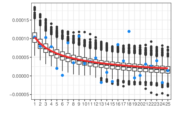
Now, let us estimate the parameters δ\delta and cc by minimizing the ℒ2\mathcal{L}^{2}-distance of τ\tau and τ^\hat{\tau} based on the first 25 time instances. We choose this value based on the computation costs of a higher threshold and on the fact that this value has proven useful in simulation studies as part of the preliminary analysis. Using our procedure, we estimate δ^=1.0474\hat{\delta}=1{\mathchar 314\relax}0474 and c^=0.0019\hat{c}=0{\mathchar 314\relax}0019. To validate our estimation, we ran a parametric bootstrap and simulated 1000 Sα^\hat{\alpha}S time series with kernel parameters δ^\hat{\delta} and c^\hat{c} to get a grasp on the variance of τ\tau in our chosen model. The results of our parametric bootstrap are depicted in Figure 3. It shows that despite some discrepancies with regard to the empirically computed τ^\hat{\tau}, which is to be expected in real data, our model exhibits a reasonable fit for the data set.

Notice that, due to the empirical estimation of the scale parameters σ\sigma and σt\sigma_{t}, it happens that τ^​(t)<0\hat{\tau}(t)<0 for some t>0t>0, which is impossible for the theoretical codifference τ\tau. This, however, does not substantially affect the quality of the fit of τ^\hat{\tau} to τ\tau. By the same parametric bootstrap we find the standard deviations of 0.18020{\mathchar 314\relax}1802 for δ\delta and 0.00050{\mathchar 314\relax}0005 for cc. It holds that δ^=1.0474<2/α=1.2821\hat{\delta}=1{\mathchar 314\relax}0474<2/\alpha=1{\mathchar 314\relax}2821 which implies by 3.7 that the log-returns of Intel Corporation are long range dependent.
Refer to caption
Figure 3: Parametric bootstrap of τ⁡(t)\tau(t). Black: boxplots of τ^​(t)\hat{\tau}(t) based on 1000 Sα^\hat{\alpha}S time series simulated with kernel parameters δ^\hat{\delta} and c^\hat{c}; Blue: τ^​(t)\hat{\tau}(t) based on data; Red: kernel function with parameters δ^\hat{\delta} and c^\hat{c} (plotted as a line for better visibility).

Data Availability Statement

The data used in this paper was provided by a free data sample from
https://www.quandl.com/data/EOD/INTC.

References

  • Asadi et al. (2015) P. Asadi, A. C. Davison, and S. Engelke. Extremes on river networks. Ann. Appl. Stat, 9(4):2023–2050, 2015.
  • Avram and Taqqu (1986) F. Avram and M. S. Taqqu. Weak convergence of moving averages with infinite variance. In Dependence in probability and statistics (Oberwolfach, 1985), volume 11 of Progr. Probab. Statist., pages 399–415. Birkhäuser Boston, Boston, MA, 1986.
  • Beran et al. (2012) J. Beran, B. Das, and D. Schell. On robust tail index estimation for linear long-memory processes. J. Time Series Anal., 33(3):406–423, 2012.
  • Beran et al. (2013) J. Beran, Y. Feng, S. Ghosh, and R. Kulik. Long memory processes. Probabilistic Properties and Statistical Methods. Springer, 2013.
  • Botcharova et al. (2014) M. Botcharova, S. F. Farmer, and L. Berthouze. Markers of criticality in phase synchronization. Front. Syst. Neurosci., 8:176, 2014.
  • Buishand et al. (2008) T. Buishand, L. De Haan, C. Zhou, et al. On spatial extremes: with application to a rainfall problem. Ann. Appl. Stat, 2(2):624–642, 2008.
  • Bulinski and Shashkin (2007) A. Bulinski and A. Shashkin. Limit Theorems for Associated Random Fields and Related Systems. World Scientific Publishing Co. Pte. Ltd., 2007.
  • Burnecki (2012) K. Burnecki. Farima processes with application to biophysical data. J. Stat. Mech. Theory Exp, 2012(05):P05015, 2012.
  • Cheung and Lai (1995) Y.-W. Cheung and K. S. Lai. A search for long memory in international stock market returns. J. Int. Money Finance, 14(4):597–615, 1995.
  • Coles (1993) S. G. Coles. Regional modelling of extreme storms via max-stable processes. J. R. Stat. Soc. Ser. B. Stat. Methodol., 55(4):797–816, 1993.
  • Damarackas and Paulauskas (2014) J. Damarackas and V. Paulauskas. Properties of spectral covariance for linear processes with infinite variance. Lith. Math. J., 54(3):252–276, 2014.
  • Damarackas and Paulauskas (2017) J. Damarackas and V. Paulauskas. Spectral covariance and limit theorems for random fields with infinite variance. J. Multivariate Anal., 153:156–175, 2017.
  • Davison and Gholamrezaee (2012) A. C. Davison and M. M. Gholamrezaee. Geostatistics of extremes. P. Roy. Soc. A-Math. Phy., 468(2138):581–608, 2012.
  • Dehling and Philipp (2002) H. Dehling and W. Philipp. Empirical process techniques for dependent data. In Empirical process techniques for dependent data, pages 3–113. Birkhäuser Boston, Boston, MA, 2002.
  • Dombry and Kabluchko (2017) C. Dombry and Z. Kabluchko. Ergodic decompositions of stationary max-stable processes in terms of their spectral functions. Stochastic Process. Appl., 127(6):1763–1784, 2017.
  • Doukhan et al. (2003) P. Doukhan, G. Oppenheim, and M. S. Taqqu, editors. Theory and applications of long-range dependence. Birkhäuser Boston, Inc., Boston, MA, 2003.
  • Embrechts et al. (1997) P. Embrechts, C. Klüppelberg, and T. Mikosch. Modelling Extremal Events for Insurance and Finance. Springer-Verlag, Berlin Heidelberg, 1997.
  • Giraitis et al. (2012) L. Giraitis, H. L. Koul, and D. Surgailis. Large sample inference for long memory processes. Imperial College Press, London, 2012.
  • Heyde and Yang (1997) C. C. Heyde and Y. Yang. On defining long-range dependence. J. Appl. Probab., 34(4):939–944, 1997.
  • Hosoya (1978) Y. Hosoya. Discrete-time stable processes and their certain properties. Ann. Probab., 6(1):94–105, 02 1978.
  • Hurst (1951) H. E. Hurst. Long-term storage capacity of reservoirs. Trans. Amer. Soc. Civil Eng., 116:770–799, 1951.
  • Jach et al. (2012) A. Jach, T. McElroy, and D. N. Politis. Subsampling inference for the mean of heavy-tailed long-memory time series. J. Time Series Anal., 33(1):96–111, 2012.
  • Kabluchko and Schlather (2010) Z. Kabluchko and M. Schlather. Ergodic properties of max-infinitely divisible processes. Stochastic Process. Appl., 120(3):281–295, 2010.
  • Kabluchko et al. (2009) Z. Kabluchko, M. Schlather, and L. de Haan. Stationary max-stable fields associated to negative definite functions. Ann. Probab., 37(5):2042–2065, 2009.
  • Kampf et al. (2020) J. Kampf, G. Shevchenko, and E. Spodarev. Nonparametric estimation of the kernel function of symmetric stable moving average random functions. Ann. Inst. Statist. Math., to appear, 2020. doi: 10.1007/510463-020-00751-6.
  • Kasahara et al. (1988) Y. Kasahara, M. Maejima, and W. Vervaat. Log-fractional stable processes. Stochastic Process. Appl., 30(2):329–339, 1988.
  • Kokoszka and Mikosch (1997) P. Kokoszka and T. Mikosch. The integrated periodogram for long-memory processes with finite or infinite variance. Stochastic Process. Appl., 66(1):55–78, 1997.
  • Kokoszka and Taqqu (1996) P. S. Kokoszka and M. S. Taqqu. Parameter estimation for infinite variance fractional ARIMA. Ann. Statist., 24(5):1880–1913, 1996.
  • Koul and Surgailis (2018) H. L. Koul and D. Surgailis. Asymptotic distributions of some scale estimators in nonlinear models with long memory errors having infinite variance. J. Time Series Anal., 39(3):273–298, 2018.
  • Kulik and Spodarev (2019) R. Kulik and E. Spodarev. Long range dependence of heavy tailed random functions. arXiv e-prints, page arXiv:1706.00742v3, 2019.
  • Lavancier (2006) F. Lavancier. Long memory random fields. In Dependence in probability and statistics, volume 187 of Lecture Notes in Statist., pages 195–220. Springer, New York, 2006.
  • Maejima and Yamamoto (2003) M. Maejima and K. Yamamoto. Long-memory stable Ornstein-Uhlenbeck processes. Electron. J. Probab., 8(19):1–18, 2003.
  • Magdziarz and Weron (2007) M. Magdziarz and A. Weron. Fractional Langevin equation with α\alpha-stable noise. A link to fractional ARIMA time series. Studia Math., 181(1):47–60, 2007.
  • McCulloch (1986) J. H. McCulloch. Simple consistent estimators of stable distribution parameters. Commun. Stat-Simul C, 15(4):1109–1136, 1986.
  • Montillet and Yu (2015) J.-P. Montillet and K. Yu. Modeling geodetic processes with Levy α\alpha-stable distribution and FARIMA. Math. Geosci., 47(6):627–646, 2015.
  • Oesting et al. (2017) M. Oesting, M. Schlather, and P. Friederichs. Statistical post-processing of forecasts for extremes using bivariate Brown–Resnick processes with an application to wind gusts. Extremes, 20(2):309–332, 2017.
  • Panas (2001) E. Panas. Estimating fractal dimension using stable distributions and exploring long memory through arfima models in athens stock exchange. Appl Financ Econ, 11(4):395–402, 2001.
  • Paulauskas (2016) V. Paulauskas. Some remarks on definitions of memory for stationary random processes and fields. Lith. Math. J., 56(2):229–250, 2016.
  • Paulauskas (1976) V. J. Paulauskas. Some remarks on multivariate stable distributions. J. Multivariate Anal., 6(3):356–368, 1976.
  • Pilipauskaitė and Surgailis (2016) V. Pilipauskaitė and D. Surgailis. Anisotropic scaling of the random grain model with application to network traffic. J. Appl. Probab., 53(3):857–879, 2016.
  • Rachev and Samorodnitsky (2002) S. T. Rachev and G. Samorodnitsky. Erratum to: “Long strange segments in a long-range-dependent moving average” [Stochastic Process. Appl. 93 (2001), no. 1, 119–148;]. Stochastic Process. Appl., 101(1):161, 2002.
  • Reed and Simon (1981) M. Reed and B. Simon. Methods of Modern Mathematical Physics, Volume 1, Functional Analysis. Academic Press, 1981.
  • Resnick (2007) S. I. Resnick. Heavy-Tail Phenomena: Probabilistic and Statistical Modeling. Springer, New York, 2007.
  • Resnick (2013) S. I. Resnick. Extreme Values, Regular Variation and Point Processes. Springer, 2013.
  • Samorodnitsky (2004) G. Samorodnitsky. Extreme value theory, ergodic theory and the boundary between short memory and long memory for stationary stable processes. Ann. Probab., 32(2):1438–1468, 2004.
  • Samorodnitsky (2016) G. Samorodnitsky. Stochastic processes and long range dependence. Springer Series in Operations Research and Financial Engineering. Springer, Cham, 2016.
  • Samorodnitsky and Taqqu (1994) G. Samorodnitsky and M. S. Taqqu. Stable non-Gaussian random processes. Stochastic Modeling. Chapman & Hall, New York, 1994. Stochastic models with infinite variance.
  • Schilling (2017) R. L. Schilling. Measures, Integrals and Martingales. Cambridge University Press, second edition, 2017.
  • Schlather (2002) M. Schlather. Models for stationary max-stable random fields. Extremes, 5(1):33–44, 2002.
  • Schlather and Tawn (2003) M. Schlather and J. A. Tawn. A dependence measure for multivariate and spatial extreme values: Properties and inference. Biometrika, 90(1):139–156, 2003.
  • Stoev (2008) S. A. Stoev. On the ergodicity and mixing of max-stable processes. Stochastic Process. Appl., 118(9):1679–1705, 2008.
  • Strokorb and Schlather (2015) K. Strokorb and M. Schlather. An exceptional max-stable process fully parameterized by its extremal coefficients. Bernoulli, 21(1):276–302, 2015.
  • Wang and Stoev (2010) Y. Wang and S. Stoev. On the structure and representations of max-stable processes. Adv. Appl. Probab., 42(3):855–877, 2010.
  • Zhang and Smith (2010) Z. Zhang and R. L. Smith. On the estimation and application of max-stable processes. J. Statist. Plann. Inference, 140(5):1135–1153, 2010.

Appendix A Appendix

Lemma A.1

Suppose UU and VV are identically distributed random variables with marginal characteristic function φU\varphi_{U} and joint characteristic function φU​V\varphi_{UV}. Also, let U′U^{\prime} and V′V^{\prime} be independent copies of UU and VV, respectively. Then, for a Fourier transform of a finite measure μ\mu denoted by ψ:ℝ→ℂ,ψ⁡(s)=∫ℝexp⁡{i​s​x}​μ​(𝑑x)\psi:\mathbb{R}\rightarrow\mathbb{C}\mathchar 24891\relax\psi(s)=\int_{\mathbb{R}}\exp\{isx\}\,\mu(dx) it holds that

𝔼​∫ℝ∫ℝf^a​(s1,s2)​ψ⁡(s1)​ψ​(s2)¯​d​s1​d​s2=∫ℝ∫ℝ𝔼​f^a​(s1,s2)​ψ⁡(s1)​ψ​(s2)¯​d​s1​d​s2,\displaystyle\mathbb{E}\int_{\mathbb{R}}\int_{\mathbb{R}}\widehat{f}_{a}(s_{1}\mathchar 24891\relax s_{2})\overline{\psi(s_{1})\psi(s_{2})}\ ds_{1}\,ds_{2}=\int_{\mathbb{R}}\int_{\mathbb{R}}\mathbb{E}\widehat{f}_{a}(s_{1}\mathchar 24891\relax s_{2})\overline{\psi(s_{1})\psi(s_{2})}\ ds_{1}\,ds_{2}\mathchar 24891\relax

where f^a​(s1,s2)=∫ℝ∫ℝei⁡(s1​u+s2​v)​fa​(u,v)​𝑑u​𝑑v\widehat{f}_{a}(s_{1}\mathchar 24891\relax s_{2})=\int_{\mathbb{R}}\int_{\mathbb{R}}e^{i(s_{1}u+s_{2}v)}f_{a}(u\mathchar 24891\relax v)\ du\,dv, a>0a>0 and

fa(u,v)=𝟙{U>u>−a,V>v>−a}−𝟙{U′>u>−a,V′>v>−a}.\displaystyle f_{a}(u\mathchar 24891\relax v)=\mathds{1}\big\{U>u>-a\mathchar 24891\relax V>v>-a\big\}-\mathds{1}\big\{U^{\prime}>u>-a\mathchar 24891\relax V^{\prime}>v>-a\big\}\mathchar 314\relax
Proof.

Let us define ga​(s1,s2)=f^a​(s1,s2)​𝟙​{s1,s2∈(−r,r)}g_{a}(s_{1}\mathchar 24891\relax s_{2})=\widehat{f}_{a}(s_{1}\mathchar 24891\relax s_{2})\mathds{1}\{s_{1}\mathchar 24891\relax s_{2}\in(-r\mathchar 24891\relax r)\} for r>0r>0 and denote

ar=∫ℝ∫ℝga​(s1,s2)​ψ⁡(s1)​ψ​(s2)¯​d​s1​d​s2=∫ℝ∫ℝg^a​(s1,s2)​μ​(s1)​μ​(s2),\displaystyle a_{r}=\int_{\mathbb{R}}\int_{\mathbb{R}}g_{a}(s_{1}\mathchar 24891\relax s_{2})\overline{\psi(s_{1})\psi(s_{2})}\ ds_{1}\,ds_{2}=\int_{\mathbb{R}}\int_{\mathbb{R}}\widehat{g}_{a}(s_{1}\mathchar 24891\relax s_{2})\ \mu(s_{1})\,\mu(s_{2})\mathchar 24891\relax

where we have used (Schilling 2017, Theorem 19.12) in the last equality and g^a\widehat{g}_{a} is the inverse Fourier transform of gag_{a}. It can be computed by tedious, yet simple calculations as

g^a​(s1,s2)\displaystyle\widehat{g}_{a}(s_{1}\mathchar 24891\relax s_{2}) =(∫−rre−i​s1​xi​x​(ei​x​U−e−i​x​a)​𝑑x)​(∫−rre−i​s2​yi​y​(ei​y​V−e−i​y​a)​𝑑y)\displaystyle=\bigg(\int_{-r}^{r}\frac{e^{-is_{1}x}}{ix}\Big(e^{ixU}-e^{-ixa}\Big)\ dx\bigg)\bigg(\int_{-r}^{r}\frac{e^{-is_{2}y}}{iy}\Big(e^{iyV}-e^{-iya}\Big)\ dy\bigg)
−(∫−rre−i​s1​xi​x​(ei​x​U′−e−i​x​a)​𝑑x)​(∫−rre−i​s2​yi​y​(ei​y​V′−e−i​y​a)​𝑑y).\displaystyle\quad-\bigg(\int_{-r}^{r}\frac{e^{-is_{1}x}}{ix}\Big(e^{ixU^{\prime}}-e^{-ixa}\Big)\ dx\bigg)\bigg(\int_{-r}^{r}\frac{e^{-is_{2}y}}{iy}\Big(e^{iyV^{\prime}}-e^{-iya}\Big)\ dy\bigg)\mathchar 314\relax (27)

Computing one of these factors gives us

∫−rre−i​s1​xi​x​(ei​x​U−e−i​x​a)​𝑑x\displaystyle\int_{-r}^{r}\frac{e^{-is_{1}x}}{ix}\Big(e^{ixU}-e^{-ixa}\Big)\ dx =∫−rr∫−aUe−i​s1​x​ei​x​t​𝑑t​𝑑x=∫−aU∫−rrei​x​(t−s1)​𝑑x​𝑑t\displaystyle=\int_{-r}^{r}\int_{-a}^{U}e^{-is_{1}x}e^{ixt}\ dt\,dx=\int_{-a}^{U}\int_{-r}^{r}e^{ix(t-s_{1})}\ dx\,dt
=2​∫r⁡(U−s1)r⁡(a−s1)1t​ei​t−e−i​t2​i​𝑑t=2​∫r⁡(U−s1)r⁡(a−s1)sin⁡tt​𝑑t<C\displaystyle=2\int_{r(U-s_{1})}^{r(a-s_{1})}\frac{1}{t}\,\frac{e^{it}-e^{-it}}{2i}\ dt=2\int_{r(U-s_{1})}^{r(a-s_{1})}\frac{\sin t}{t}\ dt<C

for some finite constant C>0C>0 which is independent of UU, VV and rr. This constant exists because the function Si​(x)=∫0xsin⁡tt​𝑑t\text{Si}(x)=\int_{0}^{x}\frac{\sin t}{t}\ dt is bounded. Thus, |g^a​(s1,s2)|≤2​C2|\widehat{g}_{a}(s_{1}\mathchar 24891\relax s_{2})|\leq 2C^{2} for all s1,s2∈ℝs_{1}\mathchar 24891\relax s_{2}\in\mathbb{R} by equality (27) and |ar|≤2​C2​μ2​(ℝ)|a_{r}|\leq 2C^{2}\mu^{2}(\mathbb{R}). Therefore, we can apply the dominated convergence theorem and 𝔼⁡[limr→∞ar]=limr→∞𝔼⁡[ar]\mathbb{E}[\lim_{r\to\infty}a_{r}]=\lim_{r\to\infty}\mathbb{E}[a_{r}]. ∎

Lemma A.2
  1. (a)

    Suppose a,b∈ℝa\mathchar 24891\relax b\in\mathbb{R} and α∈(0,2)\alpha\in(0\mathchar 315\relax 2). Then it holds that

    ||a|α+|b|α−|a−b|α|≤2​|a|α/2​|b|α/2.\displaystyle\Big||a|^{\alpha}+|b|^{\alpha}-|a-b|^{\alpha}\Big|\leq 2|a|^{\alpha/2}|b|^{\alpha/2}\mathchar 314\relax
  2. (b)

    Suppose a,b≥0a\mathchar 24891\relax b\geq 0 and α≥0\alpha\geq 0, then |a−b|α≤aα+bα|a-b|^{\alpha}\leq a^{\alpha}+b^{\alpha}.

  3. (c)

    Let α>0,a≥0,b≥0,\alpha>0\mathchar 24891\relax a\geq 0\mathchar 24891\relax b\geq 0\mathchar 24891\relax then

    ∫01∫01(a​s1+b​s2)α−|a​s1−b​s2|αs1​s2​d​s1​d​s2≥Cα​(aα∧bα),\int_{0}^{1}\int_{0}^{1}\frac{(as_{1}+bs_{2})^{\alpha}-|as_{1}-bs_{2}|^{\alpha}}{s_{1}s_{2}}\mathrm{d}s_{1}\mathrm{d}s_{2}\geq C_{\alpha}\left(a^{\alpha}\wedge b^{\alpha}\right)\mathchar 24891\relax (28)

    where Cα=2α​∫01(1+u)α−(1−u)αu​𝑑u≥4​(2α−1)α⁡(α+1).C_{\alpha}=\frac{2}{\alpha}\int_{0}^{1}\frac{(1+u)^{\alpha}-(1-u)^{\alpha}}{u}\mathrm{d}u\geq\frac{4(2^{\alpha}-1)}{\alpha(\alpha+1)}\mathchar 314\relax

Proof.
  1. (a)

    Recall that the covariance function of a fractional Brownian motion BH={BtH,t∈ℝ}B^{H}=\{B_{t}^{H}\mathchar 24891\relax t\in\mathbb{R}\} with Hurst index H∈(0,1)H\in(0\mathchar 315\relax 1) equals

    𝔼⁡[BtH​BsH]=12​(|t|2​H+|s|2​H−|t−s|2​H),\displaystyle\mathbb{E}[B_{t}^{H}B_{s}^{H}]=\frac{1}{2}(|t|^{2H}+|s|^{2H}-|t-s|^{2H})\mathchar 24891\relax (29)

    where s,t∈ℝs\mathchar 24891\relax t\in\mathbb{R}. Using the Cauchy-Schwarz inequality we have that

    |𝔼⁡[BtH​BsH]|2≤𝔼⁡[(BtH)2]​𝔼​[(BsH)2]=|t|2​H​|s|2​H.\displaystyle|\mathbb{E}[B_{t}^{H}B_{s}^{H}]|^{2}\leq\mathbb{E}[(B_{t}^{H})^{2}]\mathbb{E}[(B_{s}^{H})^{2}]=|t|^{2H}|s|^{2H}\mathchar 314\relax (30)

    Denoting α=2​H\alpha=2H and combining (29) and (30) we get |12​(|t|α+|s|α−|t−s|α)|2≤|t|α​|s|α,\bigg|\frac{1}{2}(|t|^{\alpha}+|s|^{\alpha}-|t-s|^{\alpha})\bigg|^{2}\leq|t|^{\alpha}|s|^{\alpha}\mathchar 24891\relax or, equivalently, ||t|α+|s|α−|t−s|α|≤2​|t|α/2​|s|α/2.\bigg||t|^{\alpha}+|s|^{\alpha}-|t-s|^{\alpha}\bigg|\leq 2|t|^{\alpha/2}|s|^{\alpha/2}\mathchar 314\relax

  2. (b)

    Suppose a<ba<b, then

    aα+bα−|a−b|α=aα+bα−(b−a)α≥aα+bα−bα=aα≥0.\displaystyle a^{\alpha}+b^{\alpha}-|a-b|^{\alpha}=a^{\alpha}+b^{\alpha}-(b-a)^{\alpha}\geq a^{\alpha}+b^{\alpha}-b^{\alpha}=a^{\alpha}\geq 0\mathchar 314\relax

    The claim follows analogously if a≥ba\geq b.

  3. (c)

    For simplicity, consider the case 0<a<b.0<a<b\mathchar 314\relax After the change of variable, the integral in (28) rewrites

    ∫0a∫0b(z2+z1)α−|z1−z2|αz1​z2​d​z1​d​z2=2​∬0≤z1≤z2≤a(z2+z1)α−(z2−z1)αz1​z2​d​z1​d​z2\displaystyle\int_{0}^{a}\int_{0}^{b}\frac{(z_{2}+z_{1})^{\alpha}-|z_{1}-z_{2}|^{\alpha}}{z_{1}z_{2}}\mathrm{d}z_{1}\mathrm{d}z_{2}=2\iint_{0\leq z_{1}\leq z_{2}\leq a}\frac{(z_{2}+z_{1})^{\alpha}-(z_{2}-z_{1})^{\alpha}}{z_{1}z_{2}}\mathrm{d}z_{1}\mathrm{d}z_{2}
    +∫0a∫ab(z2+z1)α−(z2−z1)αz1​z2dz2dz1≥2∫0a[∫0z2(z2+z1)α−(z2−z1)αz1dz1]d​z2z2\displaystyle+\int_{0}^{a}\int_{a}^{b}\frac{(z_{2}+z_{1})^{\alpha}-(z_{2}-z_{1})^{\alpha}}{z_{1}z_{2}}\mathrm{d}z_{2}\mathrm{d}z_{1}\geq 2\int_{0}^{a}\left[\int_{0}^{z_{2}}\frac{(z_{2}+z_{1})^{\alpha}-(z_{2}-z_{1})^{\alpha}}{z_{1}}\mathrm{d}z_{1}\right]\frac{\mathrm{d}z_{2}}{z_{2}}
    =2​∫0az2α−1​d​z2​[∫01(1+u)α−(1−u)αu​𝑑u]=Cα​aα.\displaystyle=2\int_{0}^{a}z_{2}^{\alpha-1}\mathrm{d}z_{2}\left[\int_{0}^{1}\frac{(1+u)^{\alpha}-(1-u)^{\alpha}}{u}\mathrm{d}u\right]=C_{\alpha}a^{\alpha}\mathchar 314\relax (31)

∎

Lemma A.3

Let X={X⁡(t),t∈ℝ}X=\{X(t)\mathchar 24891\relax\ t\in\mathbb{R}\} be a Sα\alphaS moving average process with parameter α∈(0,2)\alpha\in(0\mathchar 24891\relax 2), nonnegative kernel function m∈ℒα​(ℝ)m\in{\mathcal{L}}^{\alpha}(\mathbb{R}), m⁡(x)>0m(x)>0 on a set of positive Lebesgue measure and α−\alpha-spectral covariance ρt.\rho_{t}\mathchar 314\relax Let φ\varphi and φt\varphi_{t}, t∈ℝt\in\mathbb{R}, be the characteristic functions given in equations (12) and (13). Then,

I1=∫ℝ+∫ℝ+|φt​(s1,−s2)−φ⁡(s1)​φ​(s2)|s1​s2​d​s1​d​s2\displaystyle I_{1}=\int_{\mathbb{R}_{+}}\int_{\mathbb{R}_{+}}\frac{|\varphi_{t}(s_{1}\mathchar 24891\relax-s_{2})-\varphi(s_{1})\varphi(s_{2})|}{s_{1}s_{2}}\,\mathrm{d}s_{1}\,\mathrm{d}s_{2} ≤8​πα2​‖m‖α2​α​ρt‖m‖α2​α−ρt2,\displaystyle\leq\frac{8\pi}{\alpha^{2}\|m\|^{2\alpha}_{\alpha}}\frac{\rho_{t}}{\sqrt{\|m\|^{2\alpha}_{\alpha}-\rho_{t}^{2}}}\mathchar 24891\relax (32)
I2=∫ℝ+∫ℝ+|φt​(s1,s2)−φ⁡(s1)​φ​(s2)|s1​s2​d​s1​d​s2\displaystyle I_{2}=\int_{\mathbb{R}_{+}}\int_{\mathbb{R}_{+}}\frac{|\varphi_{t}(s_{1}\mathchar 24891\relax s_{2})-\varphi(s_{1})\varphi(s_{2})|}{s_{1}s_{2}}\,\mathrm{d}s_{1}\,\mathrm{d}s_{2} ≤8​πα2​‖m‖α2​α​ρt‖m‖α2​α−ρt2.\displaystyle\leq\frac{8\pi}{\alpha^{2}\|m\|^{2\alpha}_{\alpha}}\frac{\rho_{t}}{\sqrt{\|m\|^{2\alpha}_{\alpha}-\rho_{t}^{2}}}\mathchar 314\relax (33)
Proof.

First, compute for α∈(0,2)\alpha\in(0\mathchar 315\relax 2) the absolute value of the difference of characteristic functions in I1I_{1} for any s1,s2>0s_{1}\mathchar 24891\relax s_{2}>0:

|φt​(s1,−s2)−φ⁡(s1)​φ​(s2)|=φt​(s1,−s2)⋅|1−φ⁡(s1)​φ​(s2)φt​(s1,−s2)|\displaystyle|\varphi_{t}(s_{1}\mathchar 24891\relax-s_{2})-\varphi(s_{1})\varphi(s_{2})|=\varphi_{t}(s_{1}\mathchar 24891\relax-s_{2})\ \cdot\bigg|1-\frac{\varphi(s_{1})\varphi(s_{2})}{\varphi_{t}(s_{1}\mathchar 24891\relax-s_{2})}\bigg|
=φt(s1,−s2)⋅|1−exp{−∫ℝ(|s1​m​(−x)|α+|s2​m​(t−x)|α−|s1​m​(−x)−s2​m​(t−x)|α⏟≥0​ by A.2(b) )dx}|\displaystyle=\varphi_{t}(s_{1}\mathchar 24891\relax-s_{2})\cdot\bigg|1-\exp\bigg\{-\int_{\mathbb{R}}\bigg(\underbrace{|s_{1}m(-x)|^{\alpha}+|s_{2}m(t-x)|^{\alpha}-|s_{1}m(-x)-s_{2}m(t-x)|^{\alpha}}_{\geq 0\text{ by \lx@cref{creftypecap\lx@tilde refnum}{lem: inequalities_bundled}(\ref{lem: Ungleichen groesser, kleiner null}) }}\bigg)\,\mathrm{d}x\bigg\}\bigg|
≤φt​(s1,−s2)⋅∫ℝ(|s1​m​(−x)|α+|s2​m​(t−x)|α−|s1​m​(−x)−s2​m​(t−x)|α)​𝑑x\displaystyle\leq\varphi_{t}(s_{1}\mathchar 24891\relax-s_{2})\cdot\int_{\mathbb{R}}\bigg(|s_{1}m(-x)|^{\alpha}+|s_{2}m(t-x)|^{\alpha}-|s_{1}m(-x)-s_{2}m(t-x)|^{\alpha}\bigg)\,\mathrm{d}x
(by using ​|e−x−1|≤x​ for all ​x≥0)\displaystyle\hskip 227.62204pt\Big(\text{by using }|e^{-x}-1|\leq x\text{ for all }x\geq 0\Big)
≤φt(s1,−s2)⋅2s1α/2s2α/2∫ℝmα/2(−x)mα/2(t−x)dx,\displaystyle\leq\varphi_{t}(s_{1}\mathchar 24891\relax-s_{2})\cdot 2s_{1}^{\alpha/2}s_{2}^{\alpha/2}\int_{\mathbb{R}}m^{\alpha/2}(-x)m^{\alpha/2}(t-x)\,\mathrm{d}x\mathchar 24891\relax (34)

where we have used A.2(a) in the last inequality.
Similarly, we compute |φt​(s1,s2)−φ⁡(s1)​φ​(s2)||\varphi_{t}(s_{1}\mathchar 24891\relax s_{2})-\varphi(s_{1})\varphi(s_{2})| for the case α∈(1,2)\alpha\in(1\mathchar 315\relax 2) as

|φt​(s1,s2)−φ⁡(s1)​φ​(s2)|\displaystyle|\varphi_{t}(s_{1}\mathchar 24891\relax s_{2})-\varphi(s_{1})\varphi(s_{2})|
=φ⁡(s1)​φ​(s2)⋅|φt​(s1,s2)φ⁡(s1)​φ​(s2)−1|\displaystyle=\varphi(s_{1})\varphi(s_{2})\cdot\bigg|\frac{\varphi_{t}(s_{1}\mathchar 24891\relax s_{2})}{\varphi(s_{1})\varphi(s_{2})}-1\bigg|
=φ(s1)φ(s2)⋅|exp{−∫ℝ(|s1​m​(−x)+s2​m​(t−x)|α−|s1​m​(−x)|α−|s2​m​(t−x)|α⏟≥0​ since ​α>1)dx}−1|\displaystyle=\varphi(s_{1})\varphi(s_{2})\cdot\bigg|\exp\bigg\{-\int_{\mathbb{R}}\bigg(\underbrace{|s_{1}m(-x)+s_{2}m(t-x)|^{\alpha}-|s_{1}m(-x)|^{\alpha}-|s_{2}m(t-x)|^{\alpha}}_{\geq 0\text{ since }\alpha>1}\bigg)\,\mathrm{d}x\bigg\}-1\bigg|
≤φ⁡(s1)​φ​(s2)⋅∫ℝ(|s1​m​(−x)+s2​m​(t−x)|α−|s1​m​(−x)|α−|s2​m​(t−x)|α)​𝑑x\displaystyle\leq\varphi(s_{1})\varphi(s_{2})\cdot\int_{\mathbb{R}}\bigg(|s_{1}m(-x)+s_{2}m(t-x)|^{\alpha}-|s_{1}m(-x)|^{\alpha}-|s_{2}m(t-x)|^{\alpha}\bigg)\,\mathrm{d}x
≤φ(s1)φ(s2)⋅2s1α/2s2α/2∫ℝmα/2(−x)mα/2(t−x)dx\displaystyle\leq\varphi(s_{1})\varphi(s_{2})\cdot 2s_{1}^{\alpha/2}s_{2}^{\alpha/2}\int_{\mathbb{R}}m^{\alpha/2}(-x)m^{\alpha/2}(t-x)\,\mathrm{d}x
≤φt(s1,−s2)⋅2s1α/2s2α/2∫ℝmα/2(−x)mα/2(t−x)dx,\displaystyle\leq\varphi_{t}(s_{1}\mathchar 24891\relax-s_{2})\cdot 2s_{1}^{\alpha/2}s_{2}^{\alpha/2}\int_{\mathbb{R}}m^{\alpha/2}(-x)m^{\alpha/2}(t-x)\,\mathrm{d}x\mathchar 24891\relax (35)

where, again, we have used A.2(a) in the last inequality. Using the same arguments, we get for the case α∈(0,1)\alpha\in(0\mathchar 315\relax 1) that

|φt​(s1,s2)−φ⁡(s1)​φ​(s2)|=φt​(s1,s2)⋅|1−φ⁡(s1)​φ​(s2)φt​(s1,s2)|\displaystyle|\varphi_{t}(s_{1}\mathchar 24891\relax s_{2})-\varphi(s_{1})\varphi(s_{2})|=\varphi_{t}(s_{1}\mathchar 24891\relax s_{2})\ \cdot\bigg|1-\frac{\varphi(s_{1})\varphi(s_{2})}{\varphi_{t}(s_{1}\mathchar 24891\relax s_{2})}\bigg|
=φt(s1,s2)⋅|1−exp{−∫ℝ(|s1​m​(−x)|α+|s2​m​(t−x)|α−|s1​m​(−x)+s2​m​(t−x)|α⏟≥0​ since ​α<1)dx}|\displaystyle=\varphi_{t}(s_{1}\mathchar 24891\relax s_{2})\cdot\bigg|1-\exp\bigg\{-\int_{\mathbb{R}}\bigg(\underbrace{|s_{1}m(-x)|^{\alpha}+|s_{2}m(t-x)|^{\alpha}-|s_{1}m(-x)+s_{2}m(t-x)|^{\alpha}}_{\geq 0\text{ since }\alpha<1}\bigg)\,\mathrm{d}x\bigg\}\bigg|
≤φt(s1,s2)⋅2s1α/2s2α/2∫ℝmα/2(−x)mα/2(t−x)dx\displaystyle\leq\varphi_{t}(s_{1}\mathchar 24891\relax s_{2})\cdot 2s_{1}^{\alpha/2}s_{2}^{\alpha/2}\int_{\mathbb{R}}m^{\alpha/2}(-x)m^{\alpha/2}(t-x)\,\mathrm{d}x
≤φt(s1,−s2)⋅2s1α/2s2α/2∫ℝmα/2(−x)mα/2(t−x)dx,\displaystyle\leq\varphi_{t}(s_{1}\mathchar 24891\relax-s_{2})\cdot 2s_{1}^{\alpha/2}s_{2}^{\alpha/2}\int_{\mathbb{R}}m^{\alpha/2}(-x)m^{\alpha/2}(t-x)\,\mathrm{d}x\mathchar 24891\relax (36)

Now, plugging the estimates (34),(35) and (36) into I1I_{1} and I2I_{2} we get

I1,I2\displaystyle I_{1}\mathchar 24891\relax I_{2} ≤2​(∫ℝ+∫ℝ+φt​(s1,−s2)s11−α/2​s21−α/2​d​s1​d​s2)​(∫ℝmα/2​(−x)​mα/2​(t−x)​𝑑x)\displaystyle\leq 2\bigg(\int_{\mathbb{R}_{+}}\int_{\mathbb{R}_{+}}\frac{\varphi_{t}(s_{1}\mathchar 24891\relax-s_{2})}{s_{1}^{1-\alpha/2}s_{2}^{1-\alpha/2}}\,\mathrm{d}s_{1}\,\mathrm{d}s_{2}\bigg)\bigg(\int_{\mathbb{R}}m^{\alpha/2}(-x)m^{\alpha/2}(t-x)\,\mathrm{d}x\bigg)\,
=2​(∫ℝ+∫ℝ+φt​(s1,−s2)s11−α/2​s21−α/2​d​s1​d​s2)​ρt.\displaystyle=2\bigg(\int_{\mathbb{R}_{+}}\int_{\mathbb{R}_{+}}\frac{\varphi_{t}(s_{1}\mathchar 24891\relax-s_{2})}{s_{1}^{1-\alpha/2}s_{2}^{1-\alpha/2}}\,\mathrm{d}s_{1}\,\mathrm{d}s_{2}\bigg)\rho_{t}\mathchar 314\relax (37)

We estimate the integral in (37) from above via the density of a bivariate normal law. Thus,

∫ℝ+\displaystyle\int_{\mathbb{R}_{+}} ∫ℝ+φt​(s1,−s2)s11−α/2​s21−α/2​d​s1​d​s2\displaystyle\int_{\mathbb{R}_{+}}\frac{\varphi_{t}(s_{1}\mathchar 24891\relax-s_{2})}{s_{1}^{1-\alpha/2}s_{2}^{1-\alpha/2}}\,\mathrm{d}s_{1}\,\mathrm{d}s_{2}
=∫ℝ+∫ℝ+(1s1​s2)1−α2exp{−∫ℝ|s1m(−x)+(−s2)m(t−x)|αdx}ds1ds2\displaystyle=\int_{\mathbb{R}_{+}}\int_{\mathbb{R}_{+}}\bigg(\frac{1}{s_{1}s_{2}}\bigg)^{1-\tfrac{\alpha}{2}}\exp\bigg\{-\int_{\mathbb{R}}|s_{1}m(-x)+(-s_{2})m(t-x)|^{\alpha}\,\mathrm{d}x\bigg\}\mathrm{d}s_{1}\,\mathrm{d}s_{2}
=∫ℝ+∫ℝ+(1s1​s2)1−α2exp{−∫ℝ|s1m(−x)|αdx−∫ℝ|(−s2)m(t−x)|αdx\displaystyle=\int_{\mathbb{R}_{+}}\int_{\mathbb{R}_{+}}\bigg(\frac{1}{s_{1}s_{2}}\bigg)^{1-\tfrac{\alpha}{2}}\exp\bigg\{-\int_{\mathbb{R}}|s_{1}m(-x)|^{\alpha}\,\mathrm{d}x-\int_{\mathbb{R}}|(-s_{2})m(t-x)|^{\alpha}\,\mathrm{d}x
+∫ℝ|s1m(−x)|α+|(−s2)m(t−x)|α−|s1m(−x)+(−s2)m(t−x)|αdx}ds1ds2\displaystyle+\int_{\mathbb{R}}|s_{1}m(-x)|^{\alpha}+|(-s_{2})m(t-x)|^{\alpha}-|s_{1}m(-x)+(-s_{2})m(t-x)|^{\alpha}\,\mathrm{d}x\bigg\}\mathrm{d}s_{1}\,\mathrm{d}s_{2}
≤∫ℝ+∫ℝ+(1s1​s2)1−α2exp{−s1α∫ℝmα(x)dx−s2α∫ℝmα(x)dx\displaystyle\leq\int_{\mathbb{R}_{+}}\int_{\mathbb{R}_{+}}\bigg(\frac{1}{s_{1}s_{2}}\bigg)^{1-\tfrac{\alpha}{2}}\exp\bigg\{-s_{1}^{\alpha}\int_{\mathbb{R}}m^{\alpha}(x)\,\mathrm{d}x-s_{2}^{\alpha}\int_{\mathbb{R}}m^{\alpha}(x)\,\mathrm{d}x
+2(s1s2)α/2∫ℝmα/2(−x)mα/2(t−x)dx}ds1ds2\displaystyle\hskip 56.9055pt+2(s_{1}s_{2})^{\alpha/2}\int_{\mathbb{R}}m^{\alpha/2}(-x)m^{\alpha/2}(t-x)\,\mathrm{d}x\bigg\}\mathrm{d}s_{1}\,\mathrm{d}s_{2}
=∫ℝ+∫ℝ+(1s1​s2)1−α2​exp⁡{−(s1α/2​σ)2−(s2α/2​σ)2+2​ρt~​(σ​s1α/2)​(σ​s2α/2)}​d​s1​d​s2,\displaystyle=\int_{\mathbb{R}_{+}}\int_{\mathbb{R}_{+}}\bigg(\frac{1}{s_{1}s_{2}}\bigg)^{1-\tfrac{\alpha}{2}}\exp\bigg\{-(s_{1}^{\alpha/2}\sigma)^{2}-(s_{2}^{\alpha/2}\sigma)^{2}+2\tilde{\rho_{t}}(\sigma s_{1}^{\alpha/2})(\sigma s_{2}^{\alpha/2})\bigg\}\,\mathrm{d}s_{1}\,ds_{2}\mathchar 24891\relax (38)

where we denoted

σ2=ρ0=∫ℝmα​(x)​𝑑x=‖m‖αα and ρt~=ρtσ2=1σ2​∫ℝ|m⁡(−x)​m​(t−x)|α/2​𝑑x\displaystyle\sigma^{2}=\rho_{0}=\int_{\mathbb{R}}m^{\alpha}(x)\,\mathrm{d}x=\|m\|_{\alpha}^{\alpha}\quad\text{ and }\quad\tilde{\rho_{t}}=\frac{\rho_{t}}{\sigma^{2}}=\frac{1}{\sigma^{2}}\int_{\mathbb{R}}|m(-x)m(t-x)|^{\alpha/2}\,\mathrm{d}x (39)

in the last equality. Now, we have a substitution

yi2​(1−ρt~2)=σsiα/2, or si=(yiσ​2​(1−ρt~2))2/α,i=1,2,\displaystyle\frac{y_{i}}{\sqrt{2(1-\tilde{\rho_{t}}^{2})}}=\sigma s_{i}^{\alpha/2}\mathchar 24891\relax\text{ or }s_{i}=\bigg(\frac{y_{i}}{\sigma\sqrt{2(1-\tilde{\rho_{t}}^{2})}}\bigg)^{2/\alpha}\mathchar 24891\relax\quad i=1\mathchar 24891\relax 2\mathchar 24891\relax

so that

dsi=2α​yi2α−1(σ​2​(1−ρt~2))2/αdyi,i=1,2.ds_{i}=\frac{\frac{2}{\alpha}y_{i}^{\tfrac{2}{\alpha}-1}}{\big(\sigma\sqrt{2(1-\tilde{\rho_{t}}^{2})}\,\big)^{2/\alpha}}\ dy_{i}\mathchar 24891\relax\quad i=1\mathchar 315\relax 2\mathchar 314\relax

Then, relation (38) rewrites

∫ℝ+∫ℝ+((2​σ2​(1−ρt~2))2/αy12/α​y22/α)1−α2​exp⁡{−y12+y22−2​ρt~​y1​y22​(1−ρt~2)}​(2α)2y12α−1y22α−1(2​σ2​(1−ρt~2))2/α​d​y1​d​y2\displaystyle\int_{\mathbb{R}_{+}}\int_{\mathbb{R}_{+}}\bigg(\frac{\big(2\sigma^{2}(1-\tilde{\rho_{t}}^{2})\,\big)^{2/\alpha}}{y_{1}^{2/\alpha}y_{2}^{2/\alpha}}\bigg)^{1-\tfrac{\alpha}{2}}\,\exp\bigg\{-\frac{y_{1}^{2}+y_{2}^{2}-2\tilde{\rho_{t}}y_{1}y_{2}}{2(1-\tilde{\rho_{t}}^{2})}\bigg\}\,\frac{(\frac{2}{\alpha})^{{}^{2}}\,y_{1}^{\tfrac{2}{\alpha}-1}y_{2}^{\tfrac{2}{\alpha}-1}}{\big(2\sigma^{2}(1-\tilde{\rho_{t}}^{2})\,\big)^{2/\alpha}}\ dy_{1}\,dy_{2}
=(2​σ2​(1−ρt~2))−1​(2α)2​∫ℝ+∫ℝ+exp⁡{−y12+y22−2​ρt~​y1​y22​(1−ρt~2)}​d​y1​d​y2\displaystyle=\big(2\sigma^{2}(1-\tilde{\rho_{t}}^{2})\,\big)^{-1}\bigg(\frac{2}{\alpha}\bigg)^{2}\int_{\mathbb{R}_{+}}\int_{\mathbb{R}_{+}}\exp\bigg\{-\frac{y_{1}^{2}+y_{2}^{2}-2\tilde{\rho_{t}}y_{1}y_{2}}{2(1-\tilde{\rho_{t}}^{2})}\bigg\}\ dy_{1}\,dy_{2}
=4​πα2​σ2(1−ρt~2)−1/2∫0∞∫0∞12​π​1−ρt~2​exp⁡{−y12+y22−2​ρt~​y1​y22​(1−ρt~2)}​d​s1​d​s2⏟≤1​ as a density of bivariate normal distribution\displaystyle=\frac{4\pi}{\alpha^{2}\sigma^{2}}\big(1-\tilde{\rho_{t}}^{2}\,\big)^{-1/2}\underbrace{\int_{0}^{\infty}\int_{0}^{\infty}\frac{1}{2\pi\sqrt{1-\tilde{\rho_{t}}^{2}}}\exp\bigg\{-\frac{y_{1}^{2}+y_{2}^{2}-2\tilde{\rho_{t}}y_{1}y_{2}}{2(1-\tilde{\rho_{t}}^{2})}\bigg\}\,\mathrm{d}s_{1}\,ds_{2}}_{\leq 1\text{ as a density of bivariate normal distribution}}
≤4​πα2​σ2(1−ρt~2)−1/2=4​πα2​‖m‖α2​α(ρ02−ρt2)−1/2<∞ for ρt≠ρ0.\displaystyle\leq\frac{4\pi}{\alpha^{2}\sigma^{2}}\big(1-\tilde{\rho_{t}}^{2}\,\big)^{-1/2}=\frac{4\pi}{\alpha^{2}\|m\|^{2\alpha}_{\alpha}}\big(\rho_{0}^{2}-\rho_{t}^{2}\,\big)^{-1/2}<\infty\text{ for }\rho_{t}\neq\rho_{0}\mathchar 314\relax

Now, show that (ρ02−ρt2)−1/2\big(\rho_{0}^{2}-\rho_{t}^{2}\,\big)^{-1/2} is only infinite on a null set. More specifically, we show that ρt=ρ0\rho_{t}=\rho_{0} if and only if t=0t=0. Recall that the Cauchy-Schwarz inequality (cf. Reed and Simon 1981, Theorem S.3.) states that

ρt=∫ℝmα/2​(−x)​mα/2​(t−x)​𝑑x≤∫ℝmα​(−x)​𝑑x=ρ0,\displaystyle\rho_{t}=\int_{\mathbb{R}}m^{\alpha/2}(-x)m^{\alpha/2}(t-x)\,\mathrm{d}x\leq\int_{\mathbb{R}}m^{\alpha}(-x)\,\mathrm{d}x=\rho_{0}\mathchar 24891\relax

where equality holds if and only if there exists λt∈ℝ\lambda_{t}\in\mathbb{R} such that mα/2​(−x)=λt​mα/2​(t−x)​ a.em^{\alpha/2}(-x)=\lambda_{t}m^{\alpha/2}(t-x)\text{ a.e}. In this case, relation ρt=ρ0\rho_{t}=\rho_{0} yields λt=1\lambda_{t}=1. Note that due to mm being nonnegative, we can rewrite the condition as m⁡(−x)=m⁡(t−x)​ a.e.m(-x)=m(t-x)\text{ a.e.} or m⁡(x)=m⁡(x+t)​ a.e.m(x)=m(x+t)\text{ a.e.}; hence, mm is a tt-periodic function with m⁡(x)>0m(x)>0 on a set of positive Lebesgue measure which contradicts m∈ℒα​(ℝ)m\in{\mathcal{L}}^{\alpha}(\mathbb{R}) because in that case m⁡(x)→0m(x)\rightarrow 0 as x→±∞x\rightarrow\pm\infty. Consequently, ρt=ρ0\rho_{t}=\rho_{0} if and only if t=0t=0.

∎

Proof of 3.5: Let us choose μ=δ0\mu=\delta_{0} where δ0\delta_{0} is the Dirac measure concentrated at zero. Obviously this measure is finite and by 2.2 we get for t∈ℝt\in\mathbb{R}:

∫ℝ∫ℝCov(𝟙{X(0)>u},𝟙{X(t)>v})μ(du)μ(dv)\displaystyle\int_{\mathbb{R}}\int_{\mathbb{R}}\Cov(\mathds{1}\{X(0)>u\}\mathchar 24891\relax\mathds{1}\{X(t)>v\})\,\mu(\mathrm{d}u)\,\mu(\mathrm{d}v)
=12​π2​∫ℝ+∫ℝ+1s1​s2​(φt​(s1,−s2)−φt​(s1,s2))​d​s1​d​s2.\displaystyle=\frac{1}{2\pi^{2}}\int_{\mathbb{R}_{+}}\int_{\mathbb{R}_{+}}\frac{1}{s_{1}s_{2}}\bigg(\varphi_{t}(s_{1}\mathchar 24891\relax-s_{2})-\varphi_{t}(s_{1}\mathchar 24891\relax s_{2})\bigg)\,\mathrm{d}s_{1}\,\mathrm{d}s_{2}\mathchar 314\relax (40)

We denote A=|s1​m​(−x)+s2​m​(t−x)|αA=|s_{1}m(-x)+s_{2}m(t-x)|^{\alpha} and B=|s1​m​(−x)−s2​m​(t−x)|αB=|s_{1}m(-x)-s_{2}m(t-x)|^{\alpha}. Then, by ex−1≥xe^{x}-1\geq x for all x∈ℝx\in\mathbb{R} we estimate

φt​(s1,−s2)−φt​(s1,s2)\displaystyle\varphi_{t}(s_{1}\mathchar 24891\relax-s_{2})-\varphi_{t}(s_{1}\mathchar 24891\relax s_{2}) =exp{−∫ℝBdx}−exp{−∫ℝAdx}\displaystyle=\exp\bigg\{-\int_{\mathbb{R}}B\,\mathrm{d}x\bigg\}-\exp\bigg\{-\int_{\mathbb{R}}A\,\mathrm{d}x\bigg\}
=exp{−∫ℝAdx}(exp{∫ℝ[A−B]dx}−1)\displaystyle=\exp\bigg\{-\int_{\mathbb{R}}A\,\mathrm{d}x\bigg\}\bigg(\exp\bigg\{\int_{\mathbb{R}}[A-B]\,\mathrm{d}x\bigg\}-1\bigg)
≥exp{−∫ℝAdx}∫ℝ[A−B]dx.\displaystyle\geq\exp\bigg\{-\int_{\mathbb{R}}A\,\mathrm{d}x\bigg\}\int_{\mathbb{R}}[A-B]\,\mathrm{d}x\mathchar 314\relax (41)

Thus, we obtain a lower bound for the right hand side of (41):

exp{−∫ℝ|s1m(−x)+s2m(t−x)|αdx}\displaystyle\exp\bigg\{-\int_{\mathbb{R}}|s_{1}m(-x)+s_{2}m(t-x)|^{\alpha}\,\mathrm{d}x\bigg\}
×∫ℝ[(s1​m​(−x)+s2​m​(t−x))α−|s1​m​(−x)−s2​m​(t−x)|α]​𝑑x.\displaystyle\hskip 56.9055pt\times\int_{\mathbb{R}}\left[(s_{1}m(-x)+s_{2}m(t-x))^{\alpha}-|s_{1}m(-x)-s_{2}m(t-x)|^{\alpha}\right]\,\mathrm{d}x\mathchar 314\relax

Note that for any a,b>0,a\mathchar 24891\relax b>0\mathchar 24891\relax (a+b)α=((a+b)2)α/2≤2α/2​(a2+b2)α/2≤2α/2​(aα+bα).(a+b)^{\alpha}=((a+b)^{2})^{\alpha/2}\leq 2^{\alpha/2}(a^{2}+b^{2})^{\alpha/2}\leq 2^{\alpha/2}(a^{\alpha}+b^{\alpha})\mathchar 314\relax Thus, for s1,s2∈[0,1]s_{1}\mathchar 24891\relax s_{2}\in[0\mathchar 315\relax 1]

exp{−∫ℝ|s1m(−x)+s2m(t−x)|αdx}≥exp{−(s1α+s2α)2α2∥m∥αα}≥e−4​‖m‖αα.\displaystyle\exp\bigg\{-\int_{\mathbb{R}}|s_{1}m(-x)+s_{2}m(t-x)|^{\alpha}\,\mathrm{d}x\bigg\}\geq\exp\bigg\{-(s_{1}^{\alpha}+s_{2}^{\alpha})2^{\frac{\alpha}{2}}\|m\|^{\alpha}_{\alpha}\bigg\}\geq e^{-4\|m\|^{\alpha}_{\alpha}}\mathchar 314\relax

Consequently, it holds

∫0∞∫0∞1s1​s2​(φt​(s1,−s2)−φt​(s1,s2))​d​s1​d​s2≥∫01∫011s1​s2​(φt​(s1,−s2)−φt​(s1,s2))​d​s1​d​s2\displaystyle\int_{0}^{\infty}\int_{0}^{\infty}\frac{1}{s_{1}s_{2}}\bigg(\varphi_{t}(s_{1}\mathchar 24891\relax-s_{2})-\varphi_{t}(s_{1}\mathchar 24891\relax s_{2})\bigg)\,\mathrm{d}s_{1}\,\mathrm{d}s_{2}\geq\int_{0}^{1}\int_{0}^{1}\frac{1}{s_{1}s_{2}}\bigg(\varphi_{t}(s_{1}\mathchar 24891\relax-s_{2})-\varphi_{t}(s_{1}\mathchar 24891\relax s_{2})\bigg)\,\mathrm{d}s_{1}\,\mathrm{d}s_{2}
≥\displaystyle\geq ∫01∫011s1​s2(exp{−∫ℝ(s1m(−x)+s2m(t−x))αdx}\displaystyle\int_{0}^{1}\int_{0}^{1}\frac{1}{s_{1}s_{2}}\bigg(\exp\bigg\{-\int_{\mathbb{R}}(s_{1}m(-x)+s_{2}m(t-x))^{\alpha}\,\mathrm{d}x\bigg\}
×∫ℝ((s1m(−x)+s2m(t−x))α−|s1m(−x)−s2m(t−x)|α)dx)ds1ds2\displaystyle\times\int_{\mathbb{R}}\Big((s_{1}m(-x)+s_{2}m(t-x))^{\alpha}-|s_{1}m(-x)-s_{2}m(t-x)|^{\alpha}\Big)\,\mathrm{d}x\bigg)\,\mathrm{d}s_{1}\,\mathrm{d}s_{2}
≥\displaystyle\geq e−4​‖m‖αα​∫01∫01∫ℝ(s1​m​(−x)+s2​m​(t−x))α−|s1​m​(−x)−s2​m​(t−x)|αs1​s2​𝑑x​d​s1​d​s2.\displaystyle e^{-4\|m\|^{\alpha}_{\alpha}}\int_{0}^{1}\int_{0}^{1}\int_{\mathbb{R}}\frac{(s_{1}m(-x)+s_{2}m(t-x))^{\alpha}-|s_{1}m(-x)-s_{2}m(t-x)|^{\alpha}}{s_{1}s_{2}}\,\mathrm{d}x\,\mathrm{d}s_{1}\,\mathrm{d}s_{2}\mathchar 314\relax

Now, by Fubini’s theorem and A.2 (c), this is greater or equal to

e−4​‖m‖αα​Cα​∫ℝmα​(−x)∧mα​(t−x)​𝑑x.e^{-4\|m\|^{\alpha}_{\alpha}}C_{\alpha}\int_{\mathbb{R}}m^{\alpha}(-x)\wedge m^{\alpha}(t-x)\,\mathrm{d}x\mathchar 314\relax

Thus, for μ=δ0\mu=\delta_{0} we have that

∫ℝ∫ℝCov(𝟙{X(0)>u},𝟙{X(t)>v})μ(du)μ(dv)≥c∫ℝ(mα(−x)∧mα(t−x))dx.\displaystyle\int_{\mathbb{R}}\int_{\mathbb{R}}\Cov(\mathds{1}\{X(0)>u\}\mathchar 24891\relax\mathds{1}\{X(t)>v\})\,\mu(\mathrm{d}u)\,\mu(\mathrm{d}v)\geq c\int_{\mathbb{R}}\big(m^{\alpha}(-x)\wedge m^{\alpha}(t-x)\big)\,\mathrm{d}x\mathchar 314\relax

Consequently, by 1.2 and Fubini’s theorem, XX is long range dependent if

∫ℝ∫ℝ(mα​(−x)∧mα​(t−x))​𝑑x​𝑑t\displaystyle\int_{\mathbb{R}}\int_{\mathbb{R}}\big(m^{\alpha}(-x)\wedge m^{\alpha}(t-x)\big)\,\mathrm{d}x\,\mathrm{d}t =∫ℝ∫ℝ(mα​(−x)∧mα​(t−x))​𝑑t​𝑑x\displaystyle=\int_{\mathbb{R}}\int_{\mathbb{R}}\big(m^{\alpha}(-x)\wedge m^{\alpha}(t-x)\big)\,\mathrm{d}t\,\mathrm{d}x
=∫ℝ∫ℝ(mα​(x)∧mα​(t))​𝑑t​𝑑x=∞.\displaystyle=\int_{\mathbb{R}}\int_{\mathbb{R}}\big(m^{\alpha}(x)\wedge m^{\alpha}(t)\big)\,\mathrm{d}t\,\mathrm{d}x=\infty\mathchar 314\relax