Rate of Strong Convergence to Markov-modulated Brownian motion

The family of flip-flop processes corresponds to a class of piecewise-linear Markov processes that converges, in some sense, to a standard Brownian motion. Specifically, for $\lambda>0$, let $=\{\varphi^{\lambda}(t)\}_{t\geq 0}$ be a Markov jump process with state space $\{+,-\}$, initial distribution $(1/2,1/2)$ and intensity matrix

Let $r(+)=\sqrt{\lambda}$, $r(-)=-\sqrt{\lambda}$ and define

We call $\{(F^{\lambda}(t),\varphi^{\lambda}(t))\}_{t\geq 0}$ a flip-flop process. It can be shown (see, e.g., [18]) that $\mathcal{F}^{\lambda}=\{F^{\lambda}(t)\}_{t\geq 0}$ converges weakly to a standard Brownian motion $\mathcal{B}=\{B(t)\}_{t\geq 0}$ as $\lambda\rightarrow\infty$. In other words,

whenever $h:\mathcal{C}([0,\infty))\mapsto\mathds{R}$ is a bounded Borel-measurable functional continuous with respect to the topology of uniform convergence on compact intervals. Weak convergence implies that the family of probability laws induced by $\{\mathcal{F}^{\lambda}\}_{\lambda>0}$ is tight, and that, for any $0\leq t_{1}<t_{2}<\dots<t_{n}<\infty$,

These two properties are also sufficient conditions for (1.2) to hold [4]. As weak convergence is a statement regarding probability laws, the stochastic processes involved do not need to be defined on a common probability space.

An alternative definition of the flip-flop process $\mathcal{F}^{\lambda}$ is as follows. For $t>0$, let

and $N^{\lambda}(0)=0$. Then, $\{N^{\lambda}(t)\}_{t\geq 0}$ is the Poisson process of intensity $\lambda$ which counts the jumps of $\{\varphi^{\lambda}(t)\}_{t\geq 0}$, and we can rewrite (1.1) as

The process $\mathcal{F}^{\lambda}$ defined as in (1.3) was first considered in [6, 11], where a link between its transition probabilities and the telegraph equation was developed. In this context, $\mathcal{F}^{\lambda}$ became known as a telegraph process or uniform transport process, of which the weak convergence to $\mathcal{B}$ was proved in [17] and [19].

Later on, it was proved in [10] that such a convergence also holds in a pathwise sense. More precisely, the authors showed that there exists a common probability space in which the family of flip-flop (or uniform transport) processes $\{\mathcal{F}^{\lambda}\}_{\lambda>0}$ and a standard Brownian motion $\mathcal{B}$ are defined such that for any $T>0$

Whenever (1.4) holds, we say that $\mathcal{F}^{\lambda}$ converges strongly to $\mathcal{B}$ as $\lambda\rightarrow\infty$. By applying the Bounded Convergence Theorem to (1.2), we trivially get that strong convergence implies weak convergence. Strong convergence results also lead to stronger approximations for diffusions and for solutions to stochastic differential equations (e.g. in [8] and [7], respectively). In [9], the rate of strong convergence of $\mathcal{F}^{\lambda}$ to $\mathcal{B}$ was computed. The key step in [10, 9] consisted in embedding certain values of $\mathcal{F}^{\lambda}$ into $\mathcal{B}$ using the Skorokhod embedding theorem.

In recent years, the study of flip-flop processes was generalised into different directions, most of which are based on the following. Consider a process $(\mathcal{R},\mathcal{J})=\{(R(t),J(t))\}_{t\geq 0}$ where the phase process $\mathcal{J}$ is a Markov jump process on a finite state space $\mathcal{S}$, initial distribution $\bm{p}$, and intensity matrix $Q$, and the level process $\mathcal{R}$ is defined by

with $\mu_{i}\in\mathds{R}$ and $\sigma_{i}\geq 0$ for $i\in\mathcal{S}$. If $\sigma_{i}=0$ for all $i\in\mathcal{S}$, the process $(\mathcal{R},\mathcal{J})$ is known as a stochastic fluid process (SFP). If $\sigma_{i}>0$ for all $i\in\mathcal{S}$, then $(\mathcal{R},\mathcal{J})$ is called a Markov modulated Brownian motion (MMBM). In [13], it is shown that there exists a family of SFPs that converges weakly to any given MMBM. This result was later used to study MMBM with two boundaries in [12], [14] and [1], Markov-modulated sticky Brownian motion in [15], and MMBM with temporary change of regime at zero in [16].

In this paper, we construct a sequence of stochastic fluid processes which converges strongly to an MMBM of any given parameters. More specifically, we prove the following result.

In fact, Theorem 1.1 is a consequence of the following result which concerns the rate of the strong convergence of $\{(\mathcal{R}^{n},\mathcal{J}^{n})\}_{n\geq 0}$ to $(\mathcal{R},\mathcal{J})$.

The case $T\in[0,1)$ of Theorem 1.1 is a consequence of Theorem 1.2 and the Borel-Cantelli lemma, with the case $T\geq 1$ following by elementary time-scaling arguments.

This paper is structured as follows. In Section 2 we construct $(\Omega,\mathscr{F},\mathds{P})$ and describe the distributional characteristics of each stochastic fluid process $(\mathcal{R}^{n},\mathcal{J}^{n})$, for $n\geq 0$. We compute in Section 3 the rate of convergence of $\mathcal{R}^{n}$ to $\mathcal{R}$, from which the proof of Theorem 1.2, and thus that of Theorem 1.1, follows. Finally, in Section 4 we develop some implications of Theorem 1.1 regarding the downcrossing probabilities of $\mathcal{R}$ and $\mathcal{R}^{n}$; in particular, we exhibit a new link between the solutions of certain Riccati and quadratic matrix equations.

First, we construct the probability space suitable to prove Theorems 1.1 and 1.2. Fix $\bm{p}$, $Q$, $\{\mu_{i}\}_{i\in\mathcal{S}}$ and $\{\sigma_{i}>0\}_{i\in\mathcal{S}}$ of Theorem 1.1. Let $\lambda_{0}=2\max_{i\in\mathcal{S}}|Q_{ii}|$, and consider a sequence $\{\lambda_{n}\}_{n\geq 1}$ such that $\lambda_{n}\geq\lambda_{n-1}$ for $n\geq 1$ and $\lim_{n\rightarrow\infty}\lambda_{n}=\infty$. Let $(\Omega,\mathscr{F},\mathds{P})$ be a probability space that supports:

• •

  a standard Brownian motion $\mathcal{B}=\{B(t)\}_{t\geq 0}$,

• •

  a Poisson process $\mathcal{M}^{0}=\{M^{0}(t)\}_{t\geq 0}$ of rate $\lambda_{0}/2$,

• •

  a sequence of Poisson processes $\{\mathcal{\widetilde{M}}^{n}\}_{n\geq 1}$, where $\mathcal{\widetilde{M}}^{n}$ has rate $(\lambda_{n}-\lambda_{n-1})/2$,

• •

  a discrete-time Markov chain $\mathcal{X}^{0}=\{X^{0}(k)\}_{k\geq 0}$ with state space $\mathcal{S}$, initial distribution $\bm{p}$, and transition probability matrix $P_{0}:=I+(\lambda_{0}/2)^{-1}Q$,

with $\mathcal{B}$, $\mathcal{M}^{0}$, $\{\mathcal{\widetilde{M}}^{n}\}_{n\geq 1}$, and $\mathcal{X}^{0}$ being independent of each other. All the elements stated in Theorem 1.1 and of the whole manuscript will be constructed in $(\Omega,\mathscr{F},\mathds{P})$. To construct $(\mathcal{R},\mathcal{J})$ on $(\Omega,\mathscr{F},\mathds{P})$, let

The uniformization method implies that $\mathcal{J}=\{J(t)\}_{t\geq 0}$ is a Markov jump process with initial distribution $\bm{p}$ and intensity matrix $Q$. Let $\mathcal{R}=\{R(t)\}_{t\geq 0}$ be defined as on (1.5), so that $(\mathcal{R},\mathcal{J})$ corresponds to a Markov-modulated Brownian motion.

Next, for each $n\geq 0$, we construct the process $(\mathcal{R}^{n},\mathcal{J}^{n})$ as follows. Define the arrival process $\mathcal{M}^{n}=\{M^{n}(t)\}_{t\geq 0}$ to be the superposition of $\{\mathcal{M}^{0},\mathcal{\widetilde{M}}^{1},\mathcal{\widetilde{M}}^{2},\dots,\mathcal{\widetilde{M}}^{n}\}$. Then, $\mathcal{M}^{n}$ is itself a Poisson process of intensity

and its arrival epochs form a subset of the arrival epochs of $\mathcal{M}^{n+m}$ for any $m\geq 0$. In other words, $\{\mathcal{M}^{n}\}_{n\geq 0}$ is a sequence of Poisson process with nested time epochs whose new arrivals, as $n$ increases, are created independently of the existing ones. Let us emphasize that choosing to have Poissonan observations with rates $\lambda_{n}/2$ allows a direct comparison of our construction with the models of [9] and of [18] in the special case of flip-flop approximations to a standard Brownian motion.

Intuitively, our aim is to construct $(\mathcal{R}^{n},\mathcal{J}^{n})$ in such a way that $\mathcal{R}^{n}$ visits the levels of $\mathcal{R}$ inspected at the arrival epochs of the Poisson process $\mathcal{M}^{n}$. To that end, we employ the well-known Wiener-Hopf factorisation for the Brownian motion with drift; see [5, Corollary 2.4.10] for a proof.

Theorem 2.1 implies that, restricted to an exponentially distributed time interval, we can track both the value of the minimum over this period and that at the right endpoint of a Brownian motion with drift. Let $\{T_{k}^{n}\}_{k\geq 1}$ be the interarrival times of the process $\mathcal{M}^{n}$, and define $\theta_{0}^{n}:=0$,

thus $\{\theta_{k}^{n}\}_{n\geq 0}$ are the arrival epochs of $\mathcal{M}^{n}$. See Figure 1 for an illustration.

As $\{\theta_{k}^{n}\}_{n\geq 0}$ contain all the arrival epochs of $\mathcal{M}^{0}$, Equation (2.1) implies that $\{J(t)\}_{t\geq 0}$ remains constant on each interval $[\theta_{k}^{n},\theta_{k+1}^{n})$, $k\geq 0$. Consequently, given $J({\theta_{k}^{n}})=i$ on $[\theta_{k}^{n},\theta_{k+1}^{n})$, $\{R(t)\}_{t\geq 0}$ behaves like a Brownian motion with drift $\mu_{i}$ and variance $\sigma^{2}_{i}$. Thus, by sequentially using the Wiener-Hopf factorisation between arrival epochs of $\mathcal{M}^{n}$, we can keep track of $\{R(\theta_{k}^{n})\}_{k\geq 0}$ and of $\{\min_{\theta_{k}^{n}\leq t\leq\theta_{k+1}^{n}}R(t)\}_{k\geq 0}=\{\min_{0\leq t\leq T_{k+1}^{n}}R(\theta_{k}^{n}+t)\}_{k\geq 0}$ in a simple manner, which we explain in detail next.

For each $k\geq 0$, define the random variables

By Theorem 4.4 in the Appendix, $\mathcal{X}^{n}=\{X^{n}(k)\}_{k\geq 0}$ is a discrete-time Markov chain with transition probability matrix $P_{n}:=I+(\lambda_{n}/2)^{-1}Q$. The strong Markov property of $\{(R(t),J(t))\}_{t\geq 0}$ and Theorem 2.1 imply that, conditioned on $\mathcal{X}^{n}$, $\{L^{n}_{k+1}\}_{k\geq 0}$ is a collection of independent random variables. More specifically, given $X^{n}_{k}=i$, $L^{n}_{k+1}$ is exponentially distributed with rate

Similarly, $\{H^{n}_{k+1}\}_{k\geq 0}$ is a collection of conditionally independent random variables for which, given $X^{n}_{k}=i$, $H^{n}_{k+1}$ is exponentially distributed with rate

Moreover, $\{L^{n}_{k+1}\}_{k\geq 0}$ is conditionally independent of $\{H^{n}_{k+1}\}_{k\geq 0}$. Note that $\{L^{n}_{k+1}\}_{k\geq 0}$ and $\{H^{n}_{k+1}\}_{k\geq 0}$ completely describe $\{R(\theta_{k}^{n})\}_{k\geq 0}$ and $\{\min_{\theta_{k}^{n}\leq t\leq\theta_{k+1}^{n}}R(t)\}_{k\geq 0}$, in the sense that for all $k\geq 0$,

For all $k\geq 1$, if $X^{n}(k-1)=i$, define

Then, the collections $\{\widehat{L}^{n}_{k}\}_{k\geq 1}$ and $\{\widehat{H}^{n}_{k}\}_{k\geq 1}$ are i.i.d. random variables exponentially distributed with parameter $\lambda_{n}$. Let $\chi_{n}^{0}:=0$, and define for all $k\geq 1$

Let $\mathcal{J}^{n}=\{J^{n}(t)\}_{t\geq 0}$ be the process with state space $\{+,-\}\times\mathcal{S}$ defined by

Figure 2 shows a sample path of $\mathcal{J}^{n}$ with $\mathcal{S}=\{1,2,3\}$.

The process $\mathcal{J}^{n}$ jumps alternately between $\{-\}\times\mathcal{S}$ and $\{+\}\times\mathcal{S}$ with intensity given by $\lambda_{n}$; furthermore, changes in its second coordinate, which occur according to $P_{n}$, are only possible at jumps instants from $\{+\}\times\mathcal{S}$ to $\{-\}\times\mathcal{S}$. Thus, $\mathcal{J}^{n}$ is a Markov jump process with state-space $\{+,-\}\times\mathcal{S}$ (ordered lexicographically), initial distribution $(\bm{0},\bm{p})$ and intensity matrix given by

Note that the sequence of states in $\mathcal{S}$ visited by $\pi_{2}(\mathcal{J}^{n})$ coincides with that of $\mathcal{J}$, or more precisely,

Also notice the jumps of $\pi_{2}(\mathcal{J}^{n})$ can occur only at $\{\chi^{n}_{k}\}_{k\geq 0}$ while the jumps of $\mathcal{J}$ can occur only at $\{\theta^{n}_{k}\}_{k\geq 0}$. In general, $\{\chi^{n}_{k}\}_{k\geq 0}\neq\{\theta^{n}_{k}\}_{k\geq 0}$; nevertheless,

In words, the average jump times of $\pi_{2}(\mathcal{J}^{n})$ coincide with the average jump times of $\mathcal{J}$, so that the process $\pi_{2}(\mathcal{J}^{n})$ is indeed similar to $\mathcal{J}$. A more precise and stronger version of this statement is proven in Section 3.

In order to construct $\mathcal{R}^{n}$, define $r^{n}:\{+,-\}\times\mathcal{S}\mapsto\mathds{R}$ by

Let

The pair $(\mathcal{R}^{n},\mathcal{J}^{n})$ is indeed a stochastic fluid process. Moreover, from the construction of $\mathcal{J}^{n}$, (2.3) and (2.4), it follows that for all $k\geq 0$

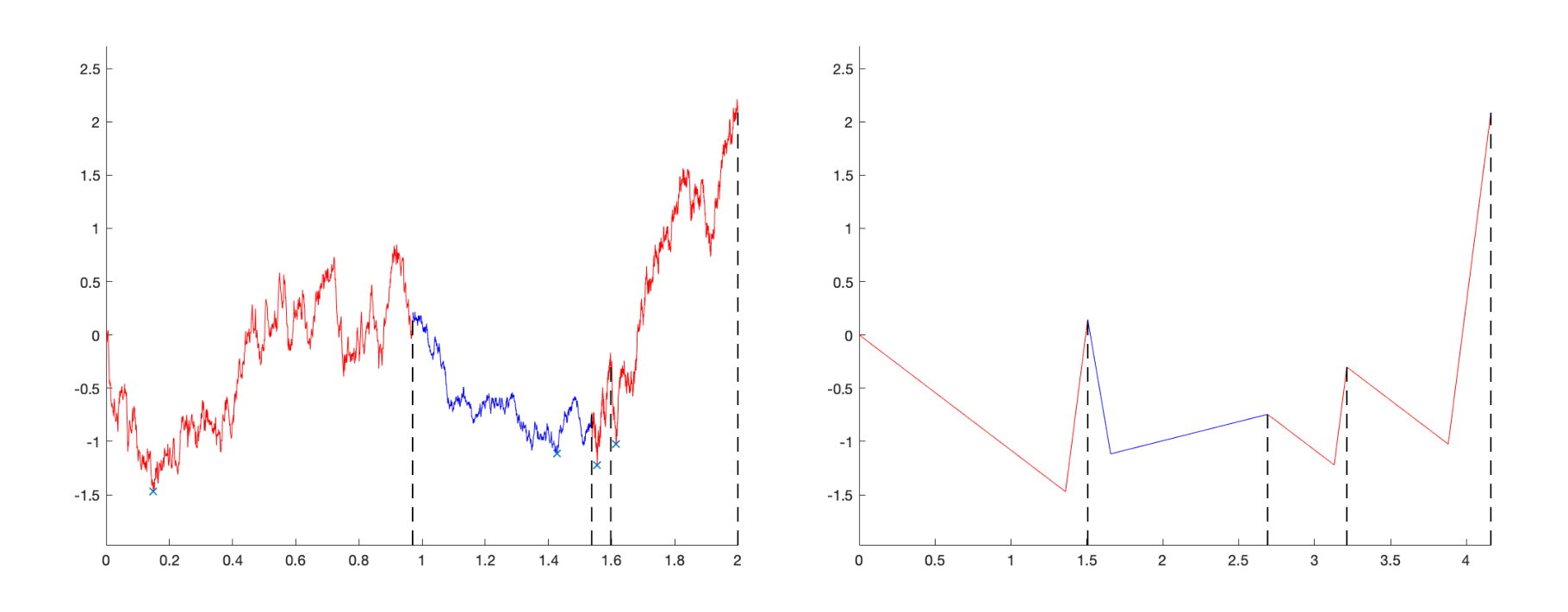
This implies that the values at the inflection points of the level process $\mathcal{R}^{n}$ coincide with the values of $\{R(\theta_{k}^{n})\}_{k\geq 0}$ and $\{\min_{\theta_{k}^{n}\leq t\leq\theta_{k+1}^{n}}R(t)\}_{k\geq 0}$. In conclusion, the values of $\mathcal{R}$ at the arrival epochs of $\mathcal{M}^{n}$, and the minimum level attained between them, are embedded in $\mathcal{R}^{n}$. Figure 3 illustrates the construction of the stochastic fluid process $(\mathcal{R}^{n},\mathcal{J}^{n})$ corresponding to the Markov-modulated Brownian motion $(\mathcal{R},\mathcal{J})$.

As $\lambda_{n}\rightarrow\infty$, the partitions induced by $\{\theta^{n}_{k}\}_{k\geq 0}$ and $\{\chi^{n}_{k}\}_{k\geq 0}$ become finer. Intuitively, this and (2.6) indicate that $\mathcal{R}^{n}$ approximates $\mathcal{R}$ as $n\rightarrow\infty$, which is stated more precisely in Theorems 1.1 and 1.2. We devote this section to rigorously prove Theorem 1.2, from which Theorem 1.1 follows as a corollary.

Let $\lambda_{n}=2n^{2}$; this makes our results and rates comparable to those of [9] and related papers. Fix $T\in[0,1)$, $q>0$ and w.l.o.g. consider $n\geq 2$ throughout.

Proof of Part (i). In order to prove (1.8), notice that

where

where $\alpha$ is a constant to be determined later. We now show that each of the quantities $P(A^{n})$ and $P(\chi_{n^{2}}^{n}<T)$ are $o(n^{-q})$.

The triangle inequality implies that

where

By (2.6), $B_{3}^{n}$ can be rewritten as

so that the events $B_{1}^{n},B_{2}^{n}$ and $B_{3}^{n}$ concern only the process $\mathcal{R}$, not $\mathcal{R}^{n}$.

Let $\{\delta_{n}\}_{n\geq 0}$ be any positive and decreasing sequence. Making a further partition, we obtain

where

On $(C^{n}_{\chi}\cup C^{n}_{\theta})^{c}$, for all $k=1,\ldots,n^{2}$ we have that

Let $x_{+}:=\max\{x,0\}$ for $x\in\mathds{R}$. If there exists $a,b\in[k/n^{2}-\delta_{n},(k+1)/n^{2}+\delta_{n}]$ such that $|R(a_{+})-R(b_{+})|>\alpha\varepsilon_{n}/4$ , then by the triangle inequality either $|R([k/n^{2}-\delta_{n}]_{+})-R(a_{+})|>\alpha\varepsilon_{n}/8$, or $|R([k/n^{2}-\delta_{n}]_{+})-R(b_{+})|>\alpha\varepsilon_{n}/8$. Therefore,

where

Thus, by (3.2) and (3.3),

In the following, we show that with an appropiate choice of $\alpha$ and $\{\delta_{n}\}_{n\geq 1}$, each summand in the RHS of (3.4) is an $o(n^{-q})$ function. For the remainder of the section, $K_{j}$, for $j\in\mathds{N}$, denote generic constants that are used to simplify bounds and are not dependent on $q$ or $n$.

Bounding $P(B^{n}_{4})$. Let $\omega_{\min}^{n}:=\min\limits_{i\in\mathcal{S}}\omega_{i}^{n},\;\eta_{\min}^{n}:=\min\limits_{i\in\mathcal{S}}\eta_{i}^{n},\;\kappa_{n}:=\omega_{\min}^{n}\wedge\eta_{\min}^{n}.$ Then,

By definition,

where the notation $O(g(n))$, for $g:\mathds{N}\mapsto\mathds{R}_{+}$, denotes a function $f:\mathds{N}\mapsto\mathds{R}$ such that $\limsup_{n\rightarrow\infty}|f(n)|/g(n)\leq M$ for some $M\in\mathds{R}$. Then, there exists $n_{1}$ such that $\kappa_{n}>n^{1/2}$ for all $n\geq n_{1}$, and so for $n\geq n_{1}$

Choose $\alpha$ to be larger than $\alpha_{1}:=8q+8$. Then, $\mathds{P}(B_{4}^{n})$ is an $O(n^{-2q})$ function and thus, it is an $o(n^{-q})$ function.

Bounding $P(C^{n}_{\chi})$ and $P(C^{n}_{\theta})$. Let $\{p_{n}\}_{n}$ be a sequence taking values in $\mathds{N}$. By Doob’s $L_{p}$-maximal inequality, we have

Since $\chi_{n^{2}}^{n}$ is a convolution of $2n^{2}$ exponential r.v.s of rate $2n^{2}$, $\chi_{n^{2}}^{n}\sim\mbox{Erlang}(2n^{2},2n^{2})$, so that (3.5) and Lemma 4.5 (in the Appendix) imply that

References

• [1] S. Ahn. Time-dependent and stationary analyses of two-sided reflected Markov-modulated Brownian motion with bilateral PH-type jumps. Journal of the Korean Statistical Society, 46(1):45–69, 2017.
• [2] S. Asmussen. Stationary distributions for fluid flow models with or without Brownian noise. Stochastic Models, 11(1):21–49, 1995.
• [3] N. G. Bean, M. M. O’Reilly, and P. G. Taylor. Algorithms for return probabilities for stochastic fluid flows. Stochastic Models, 21(1):149–184, 2005.
• [4] P. Billingsley. Convergence of Probability Measures. John Wiley & Sons, June 1999.
• [5] M. Bladt and B. F. Nielsen. Matrix-Exponential Distributions in Applied Probability, volume 81. Springer, 2017.
• [6] S. Goldstein. On diffusion by discontinuous movements, and on the telegraph equation. The Quarterly Journal of Mechanics and Applied Mathematics, 4(2):129–156, 01 1951.
• [7] L. G. Gorostiza. Rate of convergence of an approximate solution of stochastic differential equations. Stochastics, 3(1-4):267–276, 1980.
• [8] L. G. Gorostiza and R. J. Griego. Strong approximation of diffusion processes by transport processes. Journal of Mathematics of Kyoto University, 19(1):91–103, 1979.
• [9] L. G. Gorostiza and R. J. Griego. Rate of convergence of uniform transport processes to Brownian motion and application to stochastic integrals. Stochastics, 3(1-4):291–303, 1980.
• [10] R. J. Griego, D. Heath, and A. Ruiz-Moncayo. Almost sure convergence of uniform transport processes to Brownian motion. The Annals of Mathematical Statistics, 42(3):1129–1131, 1971.
• [11] M. Kac. A stochastic model related to the telegrapher’s equation. Rocky Mountain J. Math., 4(3):497–510, 09 1974.
• [12] G. Latouche and G. T. Nguyen. Fluid approach to two-sided reflected Markov-modulated Brownian motion. Queueing Systems, 80(1-2):105–125, 2015.
• [13] G. Latouche and G. T. Nguyen. The morphing of fluid queues into Markov-modulated Brownian motion. Stochastic Systems, 5(1):62–86, 2015.
• [14] G. Latouche and G. T. Nguyen. Feedback control: Two-sided Markov-modulated Brownian motion with instantaneous change of phase at boundaries. Performance Evaluation, 106:30–49, 2016.
• [15] G. Latouche and G. T. Nguyen. Slowing time: Markov-modulated Brownian motions with a sticky boundary. Stochastic Models, 33(2):297–321, 2017.
• [16] G. Latouche and M. Simon. Markov-modulated Brownian motion with temporary change of regime at level zero. Methodology and Computing in Applied Probability, pages 1–24, 2018.
• [17] M. Pinsky. Differential equations with a small parameter and the central limit theorem for functions defined on a finite markov chain. Probability Theory and Related Fields, 9(2):101–111, 1968.
• [18] V. Ramaswami. A fluid introduction to Brownian motion and stochastic integration. In Matrix-analytic methods in stochastic models, pages 209–225. Springer, 2013.
• [19] T. Watanabe. Approximation of uniform transport process on a finite interval to Brownian motion. Nagoya Mathematical Journal, 32:297–314, 1968.
• [20] R. Willink. Relationships between central moments and cumulants, with formulae for the central moments of gamma distributions. Communications in Statistics-Theory and Methods, 32(4):701–704, 2003.