Properties of Density and Velocity Gaps Induced by a Planet in a Protoplanetary Disk
Abstract
Gravitational interactions between a protoplanetary disk and its embedded planet is one of the formation mechanisms of gaps and rings found in recent ALMA observations. To quantify the gap properties measured in not only surface density but also rotational velocity profiles, we run two-dimensional hydrodynamic simulations of protoplanetary disks by varying three parameters: the mass ratio of a planet to a central star, the ratio of the disk scale height to the orbital radius of the planet, and the viscosity parameter . We find the gap depth in the gas surface density depends on a single dimensionless parameter as , consistent with the previous results of Kanagawa et al. 2015a. The gap depth in the rotational velocity is given by . The gap width, in both surface density and rotational velocity, has a minimum of about when the planet mass is around the disk thermal mass , while it increases in a power-law fashion as increases or decrease from unity. Such a minimum in the gap width arises because spirals from sub-thermal planets have to propagate before they shock the disk gas and open a gap. We compare our relations for the gap depth and width with the previous results, and discuss their applicability to observations.
Keywords:
hydrodynamics, protoplanetary disks, planet-disk interactionI Introduction
High resolution observations of protoplanetary disks in the past decade have found diverse substructures in the disks, including spiral arms (e.g., SAO 206462, Muto et al. 2012; MWC758, Grady et al. 2013; HD 100453, Wagner et al. 2015), large-scale asymmetries (e.g., HD 142527, Casassus et al. 2013; Oph IRS 48, van der Marel et al. 2013), and gaps or rings (e.g., HL Tau, ALMA Partnership et al. 2015, TW Hya: Andrews et al. 2016; HD 163296, Isella et al. 2016; HD 169142, Fedele et al. 2017; AA Tau, Loomis et al. 2017; Elias 2-24, Cieza et al. 2017; AS 209, Fedele et al. 2018; GY 91, Sheehan & Eisner 2018; V1094 Scorpii, van Terwisga et al. 2018; HD 143005, Bensity et al. 2018; HD 92945, Marino et al. 2019). Compared to other substructures in the disks, gaps or rings are nearly axisymmetric and concentric.
While these substructures appear common in protoplanetary disks, their physical origin has remained uncertain. For gaps or rings, in particular, a number of scenarios have been proposed as their formation mechanisms. For example, fast pebble growth near the snowlines of abundant volatile molecules was proposed by Zhang et al. 2015 to explain the observed gaps in HL Tau. However, the presence of eccentric rings (Dong et al. 2018a) and recent observations that gap locations do not correspond to the snowlines of the most common species in many proptoplanetary disks (Long et al. 2018; Huang et al. 2018; van der Marel et al. 2019) suggest that the snowline scenario is unlikely as a common origin of multiple gaps. Other potential mechanisms include secular gravitational instability (Takahashi & Inutsuka 2016), toroidal vortices induced by large-scale instability (Lorén-Aguilar & Bate 2016), self-induced dust vortex (Gonzalez et al. 2015), disk winds (Suriano et al. 2017), zonal flow (Flock et al. 2015), and sintering-induced piling-up of dust aggregates (Okuzumi et al. 2016). Although these mechanisms successfully produce rings at the locations close the observed ring radii in specific systems, it is unclear whether they can be applicable to all observed protoplanetary disks with gaps (Huang et al. 2018).
Perhaps, the most natural and favored mechanism for gaps/rings may be gravitational interactions between the disk and its embedded planet(s) (Lin & Papaloizou 1979). Density wakes launched by the gravity of the planet can transfer angular momentum from the regions inside the planet orbit to the outside, making the gas in the disk pushed away from the vicinity of the planet (Goldreich & Tremaine 1980; Rafikov 2002). In fact, Bae et al. 2018 showed that the disk-planet interactions with differing parameters such as viscosity and dust distribution, etc. can create diverse morphology that includes a full disk, a transition disk with an inner cavity, a disk with a single gap and a central continuum peak and a disk with multiple gap and a central continuum peak. Even a single planet can forms multiple gaps in a low-viscosity disk (Dong et al. 2017; Bae et al. 2017), because secondary and tertiary spiral arms can also grow enough to induce shocks across which gas loses its angular momentum (see also Bae & Zhu 2018; Miranda & Rafikov 2019).
The shape of a gap produced by a planet is determined by the balance between the tidal torque density and the viscous stress. In a disk with scale height and surface density around a protostar with mass , the tidal torque by a planet with mass at orbital radius is proportional to with (e.g., Goldreich & Tremaine 1980; Papaloizou & Lin 1984), while the viscous stress is proportional to the viscous parameters of Shakura & Sunayev 1973. It was shown that the gap depth in the surface density can be characterized by a single dimensionless parameter (Duffell & MacFadyen 2013; Fung et al. 2014; Kanagawa et al. 2015a), while the gap width can be described solely by (Kanagawa et al. 2016; Kanagawa et al. 2017). These relations were applied to constrain the masses of embedded planets in several systems such as HL Tau (Kanagawa et al. 2015b; Kanagawa et al. 2016), HD169142 (Kanagawa et al. 2015b), and HD 97048 (Ginski et al. 2016).
However, applying these relations for the gap depth and width to observations requires a strict assumption that the distribution of dust particles is well-matched with that of gas (Kanagawa et al. 2015b). In reality, the conversion of observed dust continuum to the gas surface density is subject to many uncertainties surrounding dust-to-gas ratio, varying dust properties, and chemical effects (Bergin et al. 2013; Miotello et al. 2017). To directly measure the gap properties in dust continuum profiles, Zhang et al. 2018 ran numerical simulations by including dust particles and obtained the empirical relations for the gap depth and width in terms of the various dimensionless parameters. But, they were still unable to incorporate dust evolution, feedback to the gas, and the potential effects of streaming instability in the simulations that may affect the gap properties significantly.
One way to circumvent the uncertainties in the gap parameters measured from the gas surface density profiles is to use the rotational velocity obtained from gas tracers such as CO that directly probes the kinematic changes in the gas disk induced by an embedded planet. Pérez et al. 2015; Pérez et al. 2018 showed that kinematic features including circumplanetary disk and large-scale velocity perturbations induced by a Jupiter-mass planet are observable with the ALMA. In fact, Teague et al. 2018 and Keppler et al. 2019 recently compared the observed rotational velocity profiles with the numerical simulations to infer the masses of planets in HD 163296 and PDS 70, respectively. Zhang et al. 2018 ran extensive numerical simulations to find an empirical relation for the amplitude of the perturbed rotational velocity as a combination of , and . Since the simulations were run up to planetary orbits, however, it is uncertain whether the gaps in their models reach a steady state, as they noted (see also Rosotti et al. 2016). In addition, they found that the width of velocity gaps is roughly 4.4 times , insensitive to and , which needs to be checked in long-term evolution.
In this paper, we run hydrodynamic simulations of protoplanetary disks to systematically investigate the gap properties in not only gas surface density profile but also rotational velocity profile induced by an embedded planet. We vary three parameters, , , and , in a wide range, and explore how the gap depth and width depend on these parameters. Our work extends Zhang et al. 2018 by exploring a wider range of the parameter space and by running the simulations 10 times longer than their models in order to achieve quasi-steady configurations of the gaps. We also introduce a new definition of the gap width in the surface density and rotational velocity profiles and provide the physical explanation for its dependence on the planet mass.
II Numerical Method
We consider a protoplanetary disk rotating at angular frequency about a central protostar with mass . The disk is assumed to be razor-thin along the vertical direction, unmagnetized, and non-self-gravitating. To study gravitational interactions between the disk with an embedded planet with mass , we run two-dimensional (2D) hydrodynamic simulations using FARGO3D in cylindrical polar coordinates (Masset 2000; Benítez-Llambay & Masset 2016). We do not consider the effects of dust and planet migration in the present work. The basic equations we solve are
| (1) | |||
| (2) |
where is the surface density, is the velocity, and is a vertically integrated gas pressure with being the isothermal speed of sound. The pressure scale height of the disk is given by , where is the angular velocity of Keplerian rotation. In Equation (2), and are the gravitational potentials of the central star and the planet located at , respectively, given by
| (3) |
where is the softening length taken equal to for . The planet is set to follow the Keplerian rotation with angular velocity , without undergoing migration. We ignore the indirect term arising from the motions of the central star relative to the center of mass of the whole system, which are shown to make insignificant differences on the gap properties (Appendix A; see also Kanagawa et al. 2017)
The last term in Equation (2) represents the viscous stress tensor
| (4) |
where is the kinematic viscosity and is the identity matrix. We adopt an -disk model of Shakura & Sunayev 1973 with , and vary to control the strength of the viscosity.
The density distribution of our initial disk follows a power-law with an exponential cutoff:
| (5) |
corresponding to a quasi-equilibrium solution of viscous disks (e.g., Lynden-Bell & Pringle 1974). The temperature profile is set to a simple power-law
| (6) |
which remains unchanged over time in our simulations. In this paper, we adopt and . These radial density and temperature distributions describe the observed protoplanetary disks reasonably well (e.g., Andrews et al. 2009; Andrews et al. 2010). We vary or to explore disks with differing temperature. In what follows, the non-uniform disks refer to a power-law disk with an exponential cutoff, in contrast to uniform disks with constant density and temperature (e.g., Kanagawa et al. 2015a; Kanagawa et al. 2016; Kanagawa et al. 2017).
The initial rotational velocity of gas in equilibrium is very close to the Keplerian velocity (within of ). Our simulation domain extends from to in radius and from 0 to in azimuth. For the boundary conditions, we adopt the wave-damping zones at and , which is known to prevent wave reflections at the boundaries (de Val-Borro et al. 2006). For simulations presented in this paper, we set up a non-uniform, logarithmically spaced cylindrical grid with radial zones and 1396 azimuthal zones. This makes the zones almost square-shaped throughout the grid (i.e., ). The grid spacing adopted here results from a compromise between computational cost and accuracy. By running simulations with various resolution, we checked that the results with agrees with those within .
The fundamental dimensional units for length, time, and mass are the orbital radius and orbital time of the planet, and the mass of the central star . Then, Equations (1) and (2) in dimensionless form depend only on three dimensionless parameters: the mass ratio , the disk aspect ratio , and the viscosity parameter . We run a total of 72 simulations that differ in these three parameters. The planet mass is varied in the range between and relative to , or between and relative to the thermal mass (e.g., Goodman & Rafikov 2001). We take , for , and for the parameter. All simulations are run up to . Table 1 in Appendix B lists the model parameters and the measured gap properties.
III Simulation Results

An introduction of the gravitational potential of a planet excites spiral waves in the disk that eventually develop into shocks. For a low-mass planet, perturbations are weak so that they propagate radially away from the planet before turning to shocks (Goodman & Rafikov 2001). When a planet is massive, however, the shock formation occurs almost instantly near the planet location. Almost inviscid disks with small may produce up to three spiral shocks, while viscious disks with large considered here form only one spiral shock (Bae et al. 2017). When the gas inside (outside) the orbit of the planet experiences a spiral shock, it loses (gains) angular momentum and thus moves inward (outward) in the radial direction, producing a gap in the surface density profile (Rafikov 2002). Similarly, the disk rotation curve, which is initially close to Keplerian, is also perturbed to become sub- and super-Keplerian in the regions with and , respectively.
The disk reaches a quasi-steady equilibrium by (see Appendix C). To quantify the gap properties, we select 11 snapshots from to , separated by a time interval , and take their time averages. We then remove the disk material, within the distance from the planet, that belongs to the spiral shocks attached to the planet rather than the gap (Fung et al. 2014). Figure 1 plots the time-averaged distribution of the normalized surface density in the – plane as well as the radial distributions of , , and for a model with (or ), , and . Here, the angle brackets denote the temporal and azimuthal average. In what follows, we first present the dependence on the input parameters of the gap depth and width in the distributions. We then discuss the depth and width in the perturbed velocity profiles.
III.1 Gap in Surface Density
Here we focus on the gap depth () and the width () in the surface density profiles and explore their dependence on the combinations of the dimensionless parameters , , and .
III.1.1 Gap Depth
Kanagawa et al. 2015a defined the gap depth in the surface density as , as illustrated in Figure 1(b). For disks with uniform density and temperature distributions, they showed that depends on , , and through a single dimensionless parameter . From the requirement that the planet-induced gravitational torque balances the viscous torque in the linear analysis, Kanagawa et al. 2015a derived the relation
| (7) |
consistent with the results of their numerical simulations for uniform disks.

To explore how the gap depth depend on in our non-uniform disks, Figure 2 plots the measured as a function of for all models. We fit the data using a functional form same as in Equation (7) but with a different coefficient. The solid line draws our least-square fit
| (8) |
to the numerical results for .11 1 Note that actually measures the height of a density floor from the bottom in the distribution. The real gap depth relative to the unperturbed value is . Equation (8) is almost equal to Equation (7), shown as the dotted line, and also to those reported by Duffell & MacFadyen 2013, Kanagawa et al. 2017, and Dong & Fung 2017. This suggests that the radial stratification in the initial disks does not affect the gap depth much. The small differences between Equation (8) (or Equation (7)) and the numerical results at for are likely due to the fact that gas responses to such massive planets are highly nonlinear, so that the linear theory of Kanagawa et al. 2015a is not applicable (see also Kanagawa et al. 2015a; Kanagawa et al. 2017; Dong & Fung 2017).
III.1.2 Gap Width
Kanagawa et al. 2016 defined the gap width as the radial distance between two points where , with the threshold value of , and showed empirically that depends on a single dimensionless parameter as
| (9) |
for uniform disks (see also Kanagawa et al. 2017). Figure 3 plots measured in our models with non-uniform disks as a functions of . To fit the data, we use a functional form same as in Equation (9) with power index fixed, and allow a proportional coefficient to vary. The solid line draws our least-square fit
| (10) |
which overall gives a wider gap, by about a factor of 1.4, than Equation (9) plotted as the dotted line. The discrepancies between and may arise from the differences in the initial distributions of the disk surface density and temperature.
Figure 3 shows that Equation (10) overestimates the width at small . This is expected since the gap width tends to decreases drastically as approaches the threshold value . In fact, the definition of Kanagawa et al. 2016 for the gap width cannot be applicable for shallow gaps with . Increasing the threshold may alleviate this problem to some extent, but at the expense of increasing the gap width.22 2 For the threshold density , our numerical results for non-uniform disks are fitted by , which can be compared with of Kanagawa et al. 2017 for uniform disks. Still, using a fixed threshold density in measuring a gap width is somewhat arbitrary and cannot be applied to all possible gaps.

We thus introduce another definition of a gap width , namely the radial distance between the points where achieves extremum values at both sides of the planet location. The new definition based on the radial gradient of the surface density is motivated to relate the gap width in the surface density to the width in the perturbed velocity profile (see Section III.2.2). We try to fit the measured using various combinations of the input parameters, and find that it is best described by the planet mass normalized by the thermal mass.
Figure 4 plots as a function of . Note that the range of is very narrow for the parameters we adopt, with on average. Still, depends weakly on the planet mass, such that it increases as decreases or increases from about 1.5. This is unlike which increase monotonically with the planet mass. We fit the data using a linear combination of two power laws in with four free parameters (two coefficients and two power indices). Our least-square fit is
| (11) |
plotted as a solid line on Figure 4. The effect of on is almost negligible compared to those of and .

The dependence of on can be understood in terms of the shock formation distance. Since perturbations induced by a low-mass planet are weak even in the regions very close to the planet, they have to travel some distance radially before undergoing nonlinear steepening into shocks. Goodman & Rafikov 2001 showed that the shock formation distance from a planet is given by
| (12) |
where is an adiabatic index. Note that the power-law dependence of on is quite similar to that of for in Equation (11). When , on the other hand, perturbations are already nonlinear over a range of radii from the planet location, instantly forming shocks there (e.g., Dong et al. 2011). In this case, the regions (i.e., gap) influenced by shocks become wider for larger .
To illustrate is associated with shocks, we calculate the azimuthally-averaged potential vorticity defined as
| (13) |
Strictly speaking, the potential vorticity in our simulations is not a conserved quantity because the initial disks are not barotropic, so that it is generated not only by the shock fronts but non-vanishing baroclinic terms. Since the potential vorticity induced by the baroclinic terms is confined to the corotation regions, its change relative to the initial profile away from the corotation is mostly caused by curved shocks. Figure 5 plots the radial distributions of (a) and (b) at for the models with differing but with the same , and . Apparently, the regions with substantial are bounded by the radii where attains its maximum or minimum, marked by the vertical dotted lines. This is observed for all simulation results which hints that for can be explained by the shock formation distance.
Figure 1 hints that the extrema in the radial gradient of occur near the bottom of a gap, making smaller than with . Figure 6 compares and with differing threshold , , , . It is apparent that is larger for larger . For most cases, is smaller than . Approximately, is similar to with , indicating that measures the width at the lower part of a gap.
III.2 Perturbed Rotational Velocity
The presence of a planet not only produces a gap in the surface density profile but also induce significant distortion in the rotational velocity . Figure 1(d) plots the exemplary distribution of the azimuthally-averaged, perturbed velocity . Clearly, the radial profile of is nearly anti-symmetric with respect to the planet, with the regions inside (outside) the planet moving slower (faster) than the initial near-Keplerian speed. In this subsection, we quantify the amplitude and width of the perturbed rotational velocity, which rapidly reach a quasi-steady state within (Appendix C).
III.2.1 Amplitude of Perturbed Velocity
We define the dimensionless amplitude, , of the perturbed rotational velocity as the difference in between the super-Keplerian peak formed near the outer gap edge and the sub-Keplerian peak near the inner gap edge, as illustrated in Figure 1(d). We measure for all models and plot as a function of in Figure 7. Apparently, the perturbed velocity is larger for a more massive planet in a colder and less diffusive disk. We try to fit using an inverse of a linear combination of two power laws in with four free parameters. The solid line draws the resulting least-square fit
| (14) |
which is within of the all measured . This predicts for .

The dependence of on and in Equation (14) results from the fact that the gaps are in hydrostatic equilibrium. In a quasi-steady state, the force balance in the radial direction reads
| (15) |
or
| (16) |
Since the pressures gradient is negative (positive) near the inner (outer) edge of the gap, the gas there should rotate slower (faster) than the initial velocity in order to maintain an equilibrium (e.g., Teague et al. 2018). Assuming that the perturbed velocity is much smaller than the initial rotation velocity and that is radially constant, one can show that Equation (16) reduces to
| (17) |
We numerically confirm that Equation (17) holds within 20% for all models, as evidenced by Figure 1(c) and (d). The deviation becomes larger as the radial range influenced by the planet increases, so that the radial dependence of becomes non-negligible. This proves that the gap width determined by the extremum positions of traces the sub/super-Keplerian peaks in the velocity profile.
Under the assumption that the profile is anti-symmetric with respect to the planet, Equation (17) gives
| (18) |
There is no obvious way to calculate at the sub- and super-Keperian peak positions, but it should be related to the gap depth and width, and scale dimensionally as .33 3 We empirically find for small . Since is a function of (Figure 2 and Equation 8) and (Figure 4), Equation (18) indicates that should be well described by the parameter alone, consistent with Figure 7.

Zhang et al. 2018 also studied the dependence on the disk parameters of the amplitude of perturbed velocities by using disk models similar to ours but without the exponential cutoff in the initial density distribution (Equation 5). They found that the amplitude of the sub/super-Keplerian peaks in the velocity profile is well fitted by
| (19) |
where . Figure 8 plots measured from our simulations as a function of . Our measured agrees, mostly within 30%, with Equation (19) plotted as a dotted line, with a small discrepancy between the two caused most likely by the difference in the initial density distribution.
III.2.2 Width of Perturbed Regions
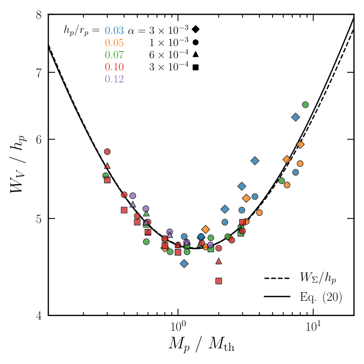
We define the width, , of the regions with significant perturbed velocities as the radial distance between the super- and sub-Keplerian peaks in the profile, as indicated in Figure 1(d). As mentioned above, would be similar to if the disks have constant temperature, but the non-uniform temperature distribution makes them slightly different from each other. Figure 9 plots as a function of . Similarly to , we fit the numerical results for using a linear combination of two power laws in with four free parameters. Our least-square fit is
| (20) |
plotted as a solid line. For comparison, we overplot Equation (11) for as a dashed line, which is very close to Equation (20), suggesting that Equation 17 is a good approximation. As in , the range of is very narrow for the parameters adopted, with on average. This is in agreement with Zhang et al. 2018 who found . Again, follows a power law for , with an index very close to , suggesting that the width of the perturbed regions is determined by the shock formation distance for a low-mass planet.
IV Discussion
So far, we have provided the quantitative dependence on the input parameters of the gap depth and width or in the perturbed density profile as well as the amplitude and spatial range of the perturbed velocities. Most observations with ALMA trace dust rather than gas in the disks, while the gap parameters measured in the present work are for the surface density and velocity distributions in the gaseous component. One thus needs to convert dust-continuum emissions to surface density maps to obtain and (Dong & Fung 2017), but the conversion process can easily be affected by the dust-to-gas ratio, dust properties, chemical effects, etc., which are quite uncertain (Bergin et al. 2013; Miotello et al. 2017). However, and are relatively free of the conversion problem because one can directly measure the perturbed rotational velocities in the gaseous disks (Pinte et al. 2018; Teague et al. 2018).
Still, the relations presented in the preceding section are based on the 2D simulations, while observed rotational velocities are derived at the emission surface of a certain tracer, which is typically above the disk midplane. To estimate the effects of the vertical disk stratification, we follow Dartois et al. 2003 and Andrews et al. 2012 to consider a thermally-stratified, axisymmetric disk in the – plane with temperature distribution
| (21) |
where is the midplane temperature (Equation 6) and is the temperature of the disk atmosphere at . We consider three models with for , 2, and 3: corresponds to an isothermal disk in .
The condition of hydrostatic equilibrium along the -direction requires that the mass density obeys
| (22) |
The force balance along the radial direction (cf. Equation 15) allows us to calculate the equilibrium rotational velocity in the – plane.
The left panels of Figure 10 plot the logarithm of the mass density in the – plane of the stratified disk models for , 2, 3 from top to bottom. The case with , , and is chosen. The right panels plot the radial distribution of at certain heights , , in comparison with the 2D results (i.e., at ). Note that the width of the perturbed regions is almost independent of . However, the amplitude of the perturbed velocity is boosted significantly as increases in a thermally-stratified disk, and the amount of the boost is proportional to through the pressure gradient in the radial direction. This suggests that the 2D results may not be applicable to optically-thick disks for which emission comes from high- regions. In this case, it is desirable to run three-dimensional simulations with radiation transfer included in order to incorporate the vertical temperature distribution as well as gas mixing induced by a planet.
With the caveat that our empirical relations are based on simulations with a single planet, we apply our empirical results to the observed rotational velocity of the C18O(2-1) emission from the HD 163296 disk presented by Teague et al. 2018. Because the inner regions of the disk suffer from insufficient spatial resolution in precisely measuring the rotational velocity (Teague et al. 2018), we focus on the outer two gaps. By using the disk temperature model of Flaherty et al. 2017, and assuming that C18O traces (Teague et al. 2018), the observed gap depth corresponds to and for the middle and outermost gaps at AU and AU, respectively.44 4 These gap locations are based on the pre-Gaia distance of to HD 163296 (van den Ancker et al. 1997). The corresponding Gaia distance is (Gaia Collaboration et al. 2018). Our empirical relation, Equation (14), then gives – and – allowing for 18% uncertainties, respectively, for middle and outermost gaps, where is the Jupiter mass. We can also place constraints on the planet mass using the observed gap width in rotation velocities. For the middle gap at 100 AU, we obtain for the observed width AU and . This suggests that the planet mass could be close to the thermal mass (), consistent with the above estimate using the gap depth relation, although we should point out that is smaller than the minimum of our best fit (4.7; Equation 20). We conjecture that this is presumably because the interaction between multiple planets could have modified the gap shape; for the middle gap in particular, it is quite possible that the gap could become narrower than otherwise, as the disk gas is pushed by both inner and outer planets. For the outer gap at 165 AU, the outer peak location cannot be well defined in the observations because the signal-to-noise ratio of the CO data drops in the outer disk (see Figure 5 of Teague et al. 2018). Depending on the exact peak location, the gap width ranges from 55 AU to 75 AU, which correspond to –. Because this covers a broad range of planet mass (Figure 9), we cannot make a meaningful estimate based on the data presented in Teague et al. 2018.
It is worth noting that the above inferred planet masses have to be regarded as a lower limit to the actual planet mass, because the observed rotation velocity deviations are smoothed with a synthesized ALMA beam and thus have to be smaller than the intrinsic values. In Teague et al. 2018, they obtained simulated CO rotation velocities by convolving the raw velocity field from a two-dimensional planet-disk interaction simulation with a synthesized ALMA beam (). Taking into the beam convolution account, they needed 1.0 and 1.3 planets to reproduce the observation, a factor of 2.3 and 1.5 larger than our estimates, respectively. These discrepancies between the planet mass with and without beam convolution suggest that one should be careful when applying our relation for directly to observations.
As a measure of gap width in real observations, Zhang et al. 2018 suggested the width normalized by the location of the outer gap edge instead of the planet position since the latter is hardly constrained observationally. Assuming that the density gap is symmetric with respect to the planet, one can express in terms of as
| (23) |
and a similar expression for the spatial width of the regions with significant velocity perturbations. Using our simulations, we check that Equation (23) is accurate within 8%, suggesting that the is nearly symmetric relative to the planet.
In this paper, we have explored various gap properties produced by planets using simple numerical simulations. There are certainly many caveats that need to be improved in future studies. Our models consider only gaseous disks and neglect the effects of dust. A dust-gas mixture is prone to streaming instability (Youdin & Goodman 2005) and the gap structure can be altered by the frictional feedback of dust when a sufficient amount of dust is trapped at the edge of the gap (Kanagawa et al. 2018). In addition, our simulations do not allow for planet migration by taking a fixed circular orbit. Nazari et al. 2019 showed that the number and shape of gaps depend on the migration speed of a planet and the drift speed of dust. Also, increasing an inclination angle of the planet orbit relative to the disk midplane tends to make a gap shallower (Zhu 2018).
Our models adopt viscous disks with , so that we are unable to explore multiple gaps launched by a single planet commonly found in low viscosity disks with (Dong et al. 2017; Bae et al. 2017). A number of studies investigated the spacing, depth, and number of gaps (Dong et al. 2018b; Zhang et al. 2018), but other gap parameters such as the gap depth in the surface profile and the properties of the associated velocity have yet to be explored for multiple gaps. Comparison of the properties between primary and secondary gaps would help distinguish whether observed multiple gaps are launched by a single or multiple planets.
Finally, our simulations do not include the effects of magnetic fields that may be pervasive in protoplanetary disks. Previous work that ran magnetohydrodynamic simulations of protoplanetary disks reported that gap structure can be changed considerably by magnetic fields (Winters et al. 2003; Nelson & Papaloizou 2003; Uribe et al. 2011; Zhu et al. 2013). The presence of magnetic fields tends to make gaps wider compared to unmagnetized counterparts, there is no consensus on the effect of magnetic fields on the gap depth. For instance, Winters et al. 2003 with toroidal fields reported that turbulence driven by magnetorotational instability makes the gaps shallower, while Nelson & Papaloizou 2003 and Zhu et al. 2013 with initial poloidal fields found turbulence makes the gaps deeper that the hydrodynamic cases. It is uncertain whether the discrepancies in the results with magnetic fields are due to filed geometry, disk structure, numerical methods, or resolution. This issue will be addressed by comparing the results of simulations in which one one parameter is varied, while the other parameters are fixed.
V Summary
We run 2D hydrodynamic simulations of protoplanetary disks with an embedded planet to study the properties of gaps in the surface density profile and the perturbed rotational velocity induced by the planet. We assume that the disks are razor thin, locally isothermal, unmagnetized, non-self-gravitating, and non-uniform in the radial direction. To investigate various situations, we vary the mass ratio of a planet to a central star, the ratio of the disk scale height to the orbital radius of the planet, and the viscosity parameter . We measure the gap depth and width in the surface density and velocity profiles after when a system reaches a quasi-steady state, and fit them using various combinations of the input parameters. Our main results can be summarized as follows.
- 1.
The gap depth in the surface density profile in our non-uniform disks is well described by the parameter introduced by Kanagawa et al. 2015a as (see Equation 8 and Figure 2), which is very close to the well-known relation of Kanagawa et al. 2015a for uniform disks.
- 2.
The gap width defined as the radial distance between two points with behaves as (see Equation 10 and Figure 3), where is a dimensionless parameter introduced by Kanagawa et al. 2016. Gaps in our non-uniform disks are wider than those in uniform disks by a factor of .
- 3.
An alternative gap width based on the radial gradient of the surface density profile has a minimum at , while depending weakly on as , with being the thermal mass (see Equation 11 and Figure 4). The power-law dependence of on suggests that the gap formation involves nonlinear steepening of perturbations into shocks for low-mass planets.
- 4.
The dimensionless amplitude of the perturbed rotational velocity , defined as the difference between the positive peak and the negative peak in the profile can be parameterized by as (see Equation 14 and Figure 7). The perturbed rotational velocity is directly related to the radial gradient of the surface density profile via Equation (17).
- 5.
These parameterized gap properties can be applied to observations to infer the planet mass and orbital radius as well as the disk properties that are difficult to constrain observationally, for gaps produced by planets.
Appendix A Effects of the Indirect Term
To illustrate the effects of the indirect term () arising from the motion of the central star relative to the center of mass, we run a simulation for , and by including the indirect term in the momentum equations. Figure 11 compares the radial distributions of the normalized surface density and the normalized perturbed velocity averaged over the azimuthal direction and time – between the cases with and without the indirect term. The indirect term make almost negligible (less than 1%) changes to the gap profiles, consistent with the results of Kanagawa et al. 2017 that the indirect term do not significantly contribute to the angular momentum flux of waves generated by a planet. This confirms that one can ignore the indirect term in measuring the gap properties.
Appendix B Model Parameters and Measured Gap Properties
Table 1 lists the model parameters and gap properties measured from the radial distributions of and averaged over the azimuthal direction and over –. Columns (1)–(3) give the disk aspect ratio , viscosity parameter , and mass ratio , respectively. Columns (4)–(6) give the depth from the bottom in the distribution, width defined by the radial distance between two points where , and width defined by the distance between minimum and maximum points in the distribution. Columns (7) and (8) give the depth and width width defined by the difference in and the radial distance between the super- and sub-Keplerian peaks. All quantities are dimensionless.
| aa can be calculated only when . | |||||||
|---|---|---|---|---|---|---|---|
| (1) | (2) | (3) | (4) | (5) | (6) | (7) | (8) |
| 0.03 | 1 | 3.0 | 3.99 | 0.121 | 0.144 | 9.37 | 0.144 |
| 4.0 | 2.87 | 0.157 | 0.144 | 1.32 | 0.144 | ||
| 6.0 | 1.63 | 0.201 | 0.153 | 1.91 | 0.149 | ||
| 8.0 | 9.72 | 0.232 | 0.153 | 2.41 | 0.153 | ||
| 1.0 | 5.91 | 0.263 | 0.158 | 2.86 | 0.158 | ||
| 2.0 | 5.75 | 0.428 | 0.167 | 4.79 | 0.167 | ||
| 3 | 3.0 | 5.77 | – | 0.144 | 4.16 | 0.135 | |
| 4.0 | 4.76 | 0.078 | 0.144 | 6.40 | 0.144 | ||
| 6.0 | 3.35 | 0.152 | 0.153 | 1.02 | 0.153 | ||
| 8.0 | 2.42 | 0.188 | 0.162 | 1.35 | 0.162 | ||
| 1.0 | 1.76 | 0.224 | 0.171 | 1.66 | 0.171 | ||
| 2.0 | 3.84 | 0.337 | 0.189 | 3.01 | 0.189 | ||
| 0.05 | 1 | 1.0 | 3.84 | 0.234 | 0.238 | 1.36 | 0.238 |
| 2.0 | 1.51 | 0.368 | 0.238 | 3.05 | 0.234 | ||
| 3.0 | 7.24 | 0.455 | 0.248 | 4.20 | 0.239 | ||
| 4.0 | 3.71 | 0.543 | 0.248 | 5.18 | 0.248 | ||
| 5.0 | 1.96 | 0.636 | 0.253 | 6.09 | 0.253 | ||
| 8.0 | 3.06 | 0.889 | 0.272 | 8.35 | 0.270 | ||
| 1.0 | 6.58 | 1.088 | 0.271 | 9.59 | 0.284 | ||
| 3 | 1.0 | 5.63 | – | 0.234 | 6.11 | 0.234 | |
| 2.0 | 3.13 | 0.267 | 0.252 | 1.70 | 0.244 | ||
| 4.0 | 1.24 | 0.415 | 0.270 | 3.25 | 0.262 | ||
| 8.0 | 2.33 | 0.640 | 0.284 | 5.71 | 0.286 | ||
| 1.0 | 1.06 | 0.742 | 0.294 | 6.61 | 0.297 | ||
| 0.07 | 3 | 2.0 | 2.61 | 0.414 | 0.349 | 3.16 | 0.345 |
| 4.0 | 8.27 | 0.541 | 0.324 | 6.17 | 0.329 | ||
| 6.0 | 3.39 | 0.645 | 0.330 | 8.00 | 0.326 | ||
| 1.0 | 7.37 | 0.882 | 0.335 | 1.06 | 0.338 | ||
| 6 | 2.0 | 3.53 | 0.369 | 0.349 | 2.10 | 0.354 | |
| 5.0 | 8.81 | 0.568 | 0.325 | 5.65 | 0.330 | ||
| 1.0 | 1.72 | 0.800 | 0.339 | 8.97 | 0.341 | ||
| 1 | 1.0 | 6.79 | – | 0.386 | 4.21 | 0.386 | |
| 2.0 | 4.29 | 0.278 | 0.332 | 1.53 | 0.332 | ||
| 3.0 | 2.71 | 0.408 | 0.324 | 2.80 | 0.324 | ||
| 4.0 | 1.82 | 0.469 | 0.324 | 3.89 | 0.324 | ||
| 6.0 | 9.22 | 0.563 | 0.329 | 5.50 | 0.335 | ||
| 8.0 | 5.10 | 0.649 | 0.335 | 6.75 | 0.336 | ||
| 1.0 | 2.96 | 0.728 | 0.339 | 7.83 | 0.343 | ||
| 2.0 | 2.80 | 1.148 | 0.385 | 1.19 | 0.382 | ||
| 3.0 | 1.36 | 1.649 | 0.451 | 1.39 | 0.455 | ||
| 0.10 | 3 | 3.0 | 4.74 | 0.244 | 0.541 | 2.19 | 0.546 |
| 4.0 | 3.40 | 0.496 | 0.517 | 3.48 | 0.510 | ||
| 5.0 | 2.49 | 0.583 | 0.493 | 4.75 | 0.496 | ||
| 6.0 | 1.90 | 0.620 | 0.485 | 5.92 | 0.485 | ||
| 8.0 | 1.24 | 0.675 | 0.469 | 7.74 | 0.470 | ||
| 1.0 | 8.68 | 0.712 | 0.463 | 9.00 | 0.463 | ||
| 2.0 | 1.82 | 0.865 | 0.432 | 1.35 | 0.433 | ||
| 3.0 | 7.95 | 0.991 | 0.488 | 1.62 | 0.496 | ||
| 6 | 3.0 | 5.73 | – | 0.560 | 1.35 | 0.565 | |
| 6.0 | 2.86 | 0.558 | 0.485 | 4.12 | 0.485 | ||
| 1.0 | 1.42 | 0.676 | 0.474 | 7.15 | 0.470 | ||
| 2.0 | 3.84 | 0.813 | 0.458 | 1.13 | 0.453 | ||
| 1 | 3.0 | 6.42 | – | 0.591 | 9.33 | 0.583 | |
| 4.0 | 5.40 | – | 0.529 | 1.56 | 0.528 | ||
| 5.0 | 4.49 | 0.349 | 0.509 | 2.28 | 0.503 | ||
| 6.0 | 3.74 | 0.470 | 0.491 | 3.02 | 0.496 | ||
| 8.0 | 2.68 | 0.565 | 0.478 | 4.46 | 0.478 | ||
| 1.0 | 2.00 | 0.620 | 0.478 | 5.69 | 0.470 | ||
| 1.5 | 1.08 | 0.707 | 0.466 | 8.03 | 0.472 | ||
| 2.0 | 6.25 | 0.767 | 0.468 | 9.78 | 0.467 | ||
| 2.5 | 3.85 | 0.826 | 0.471 | 1.13 | 0.476 | ||
| 3.0 | 2.44 | 0.885 | 0.478 | 1.26 | 0.486 | ||
| 0.12 | 6 | 8.0 | 3.55 | 0.573 | 0.627 | 3.96 | 0.620 |
| 1.0 | 2.68 | 0.676 | 0.603 | 5.39 | 0.595 | ||
| 1.5 | 1.55 | 0.782 | 0.578 | 8.31 | 0.578 | ||
| 2.0 | 1.05 | 0.841 | 0.568 | 1.01 | 0.568 | ||
| 1 | 8.0 | 4.52 | 0.381 | 0.633 | 2.85 | 0.632 | |
| 1.0 | 3.60 | 0.561 | 0.608 | 3.99 | 0.614 | ||
| 1.5 | 2.20 | 0.720 | 0.577 | 6.59 | 0.582 | ||
| 2.0 | 1.51 | 0.783 | 0.572 | 8.74 | 0.568 | ||
| 3.0 | 7.49 | 0.878 | 0.559 | 1.12 | 0.564 |
Appendix C Temporal Changes of the Gap Properties
To explore how the gap properties change with time, we select a model with , and and measure the depth and width of the surface density gap and the depth and width of the velocity gap at every starting from to . Figure 12 plots the resulting temporal variations of (a) and and (b) and . The properties of the density gap converge to relatively slowly with time to quasi-steady values reached at around . In this model, and at are about times larger and times smaller than the values at , respectively. Interestingly, the gap properties in the velocity profiles converge rapidly within : relative differences of and between and are only 1.3% and 0.22%, respectively. In our simulations, the density profile deepens secularly with time, while retaining its radial gradient as well as the corresponding velocity profile intact.
References
- ALMA Partnership et al. (2015) ALMA Partnership, Brogan, C. L., Pérez, L. M., et al. 2015, ApJ, 808, L3
- Andrews et al. (2009) Andrews, S. M., Wilner, D. J., Hughes, A. M., Qi, C., Dullemond, C. P. 2009, ApJ, 700, 1502
- Andrews et al. (2010) Andrews, S. M., Wilner, D. J., Hughes, A. M., Qi, C., Dullemond, C. P. 2010, ApJ, 723, 124
- Andrews et al. (2012) Andrews, S. M., Wilner, D. J., Hughes, A. M., et al. 2012, ApJ, 744, 162
- Andrews et al. (2016) Andrews, S. M., Wilner, D. J., Zhu, Z., et al. 2016, ApJ, 820, L40
- Bae et al. (2017) Bae, J., Zhu, Z., & Hartmann, L. 2017, ApJ, 850, 201
- Bae & Zhu (2018) Bae, J., & Zhu, Z. 2018, ApJ, 859, 118
- Bae et al. (2018) Bae, J., Pinilla, P., & Birnstiel, T. 2018, ApJ, 864, L26
- Benítez-Llambay & Masset (2016) Benítez-Llambay, P., & Masset, F. 2016, ApJS, 223, 11
- Bensity et al. (2018) Benisty, M., Juhász, A., Facchini, S., et al. 2018, A&A, 619, A171
- Bergin et al. (2013) Bergin, E. A., Cleeves, L. I., Gorti, U., et al. 2013, Nature, 493, 644.
- Casassus et al. (2013) Casassus, S., van der Plas, G., S, P. M., et al. 2013, Nature, 493, 191
- Cieza et al. (2017) Cieza, L. A., Casassus, S., Pérez, S., et al. 2017, ApJ, 851, L23
- de Val-Borro et al. (2006) de Val-Borro, M., Edgar, R. G., Artymowicz, P., et al. 2006, MNRAS, 370, 529
- Dartois et al. (2003) Dartois, E., Dutrey, A., & Guilloteau, S. 2003, A&A, 399, 773
- Dong et al. (2011) Dong, R., Rafikov, R. R., & Stone, J. M. 2011,ApJ, 741, 57
- Dong & Fung (2017) Dong, R., & Fung, J. 2017, ApJ, 835, 146
- Dong et al. (2017) Dong, R., Li, S., Chiang, E., & Li, H. 2017, ApJ, 843, 127
- Dong et al. (2018a) Dong, R., Liu, S.-y., Eisner, J., et al. 2018a, ApJ, 860, 124
- Dong et al. (2018b) Dong, R., Li, S., Chiang, E., Li, H. 2018b, ApJ, 866, 110
- Duffell & MacFadyen (2013) Duffell, P. C., & MacFadyen, A. I. 2013, ApJ, 769, 41
- Fedele et al. (2017) Fedele, D., Carney, M., Hogerheijde, M. R., et al. 2017, A&A, 600, A72
- Fedele et al. (2018) Fedele, D., Tazzari, M., Booth, R., et al. 2018, A&A, 610, A24
- Flaherty et al. (2017) Flaherty, K. M., Hughes, A. M., Rose, S. C., et al. 2017, ApJ, 843, 150
- Flock et al. (2015) Flock, M., Ruge, J. P., Dzyurkevich, N., et al. 2015, A&A, 574, A68
- Fung et al. (2014) Fung, J., Shi, J.-M., & Chiang, E. 2014, ApJ, 782, 88
- Gaia Collaboration et al. (2018) Gaia Collaboration, Brown, A. G. A., Vallenari, A., et al. 2018, A&A, 616, A1
- Ginski et al. (2016) Ginski, C., Stolker, T., Pinilla, P., et al. 2016, A&A, 595, A112
- Goldreich & Tremaine (1980) Goldreich, P., & Tremaine, S. 1980, ApJ, 241, 425
- Gonzalez et al. (2015) Gonzalez, J.-F., Laibe, G., Maddison, S. T., Pinte, C., & Ménard, F. 2015, MNRAS, 454, L36
- Goodman & Rafikov (2001) Goodman, J., & Rafikov, R. R. 2001, ApJ, 552, 793
- Grady et al. (2013) Grady, C. A., Muto, T., Hashimoto, J., et al. 2013, ApJ, 762, 48
- Huang et al. (2018) Huang, J., Andrews, S. M., Dullemond, C. P., et al. 2018, ApJ, 869, L42
- Isella et al. (2016) Isella, A., Guidi, G., Testi, L., et al. 2016, Phys. Rev. Lett., 117, 251101
- Johansen et al. (2014) Johansen, A., Blum, J., Tanaka, H., et al. 2014, in Protostars and Planets VI, ed. H. Beuther et al. (Tucson, AZ: Univ. Arizona Press), 547
- Kanagawa et al. (2015a) Kanagawa, K. D., Tanaka, H., Muto, T., Tanigawa, T., & Takeuchi, T. 2015b, MNRAS, 448, 994
- Kanagawa et al. (2015b) Kanagawa, K. D., Muto, T., Tanaka, H., et al. 2015a, ApJ, 806, L15
- Kanagawa et al. (2016) Kanagawa, K. D., Muto, T., Tanaka, H., et al. 2016, PASJ, 68, 43
- Kanagawa et al. (2017) Kanagawa, K. D., Tanaka, H., Muto, T., & Tanigawa, T. 2017, PASJ, 69, 97
- Kanagawa et al. (2018) Kanagawa, K. D., Muto, T., Okuzumi, S., et al. 2018, ApJ, 868, 48
- Keppler et al. (2019) Keppler, M., Teague, R., Bae., J., et al. 2019, A&A, 625, A118
- Li et al. (2005) Li, H., Li, S., Koller, J., et al. 2005, ApJ, 624, 1003
- Lin & Papaloizou (1979) Lin, D. N. C., & Papaloizou, J. 1979, MNRAS, 188, 191
- Lin & Papaloizou (1986) Lin, D. N. C., & Papaloizou, J. 1986, ApJ, 307, 395
- Liu et al. (2018) Liu, S.-F., Jin, S., Li, S., et al. 2018, ApJ, 857, 87
- Long et al. (2018) Long, F., Pinilla, P., Herczeg, G. J., et al. 2018, ApJ, 869, 17
- Loomis et al. (2017) Loomis, R. A., Öberg, K. I., Andrews, S. M., & MacGregor, M. A. 2017, ApJ, 840, 23
- Lorén-Aguilar & Bate (2016) Lorén-Aguilar, P., & Bate, M. R. 2016, MNRAS, 457, L54
- Lynden-Bell & Pringle (1974) Lynden-Bell, D., & Pringle, J. E. 1974, MNRAS, 168, 603
- Marino et al. (2019) Marino, S., Yelverton, B., Booth, M., et al. 2019, MNRAS, 484, 1257
- Masset (2000) Masset, F. 2000, A&AS, 141, 165
- Miranda & Rafikov (2019) Miranda, R., & Rafikov, R. R. 2019, ApJ, 515, 767
- Miotello et al. (2017) Miotello, A., van Dishoeck, E. F., Williams, J. P., et al. 2017, A&A, 599, A113.
- Muto et al. (2012) Muto, T., Grady, C. A., Hashimoto, J., et al. 2012, ApJ, 748, L22
- Nazari et al. (2019) Nazari, P., Booth., R. A., Clarke, C. J., et al. 2019, MNRAS, 485, 5914
- Nelson & Papaloizou (2003) Nelson, R. P., & Papaloizou, J. C. B. 2003, MNRAS, 339, 993
- Okuzumi et al. (2016) Okuzumi, S., Momose, M., Sirono, S.-i., Kobayashi, H., & Tanaka, H. 2016, ApJ, 821, 82
- Papaloizou & Lin (1984) Papaloizou, J., & Lin, D. N. C. 1984, ApJ, 285, 818
- Pérez et al. (2015) Pérez, S., Dunhill, A., Casassus, S., et al. 2015, ApJ, 811, L5
- Pérez et al. (2018) Pérez, S., Casassus, S., & Benítez-Llambay, P. 2018, MNRAS, 480, L12
- Pinte et al. (2018) Pinte, C., Price, D. J., Ménard, F., et al. 2018, ApJ, 860, L13
- Rafikov (2002) Rafikov, R. R. 2002, ApJ, 572, 566
- Rosotti et al. (2016) Rosotti, G. P., Juhasz, A., Booth, R. A., & Clarke, C. J. 2016, MNRAS, 459, 2790
- Shakura & Sunayev (1973) Shakura, N. I., & Sunyaev, R. A. 1973, A&A, 24, 337
- Suriano et al. (2017) Suriano, S. S., Li, Z.-Y., Krasnopolsky, R., & Shang, H. 2017, MNRAS, 468, 3850
- Sheehan & Eisner (2018) Sheehan, P. D., & Eisner, J. A. 2018, ApJ, 857, 18
- Takahashi & Inutsuka (2016) Takahashi, S. Z., & Inutsuka, S.-i. 2016, AJ, 152, 184
- Teague et al. (2018) Teague, R., Bae, J., Bergin, E., Birnstiel, T.,& Foreman-Mackey, D. 2018, ApJ, 860, L12
- Uribe et al. (2011) Uribe, A. L., Klahr, H., Flock, M., & Henning, T. 2011, ApJ, 736, 85
- van den Ancker et al. (1997) van den Ancker M. E., The, P. S., Tjin A Djie, H. R. E., et al., 1995, A&A, 324, L33
- van der Marel et al. (2013) van der Marel, N., van Dishoeck, E. F., Bruderer, S. et al. 2013, Science, 340,1199
- van der Marel et al. (2019) van der Marel, N., Dong, R., di Francesco, J., et al. 2019, ApJ, 872, 112
- van Terwisga et al. (2018) van Terwisga, S. E., van Dishoeck, E. F., Ansdell, M., et al. 2018, A&A, 616, A88
- Wagner et al. (2015) Wagner, K., Apai, D., Kasper, M., & Robberto, M. 2015, ApJ, 813, L2
- Winters et al. (2003) Winters, W. F., Balbus, S. A.,& Hawley, J. F. 2003, ApJ, 589, 543
- Youdin & Goodman (2005) Youdin, A. N., & Goodman, J. 2005, ApJ, 620, 459,
- Zhang et al. (2015) Zhang, K., Blake, G. A., & Bergin, E. A. 2015, ApJ, 806, L7
- Zhang et al. (2018) Zhang, S., Zhu, Z., Huang, J. et al. 2018, ApJ, 869, L47
- Zhu et al. (2013) Zhu, Z., Stone, J. M.,& Rafikov, R. R. 2013, ApJ, 768, 143
- Zhu (2018) Zhu, Z. 2018, MNRAS, 483, 4221