Implications of pinned occupation numbers for natural orbital expansions. I: Generalizing the concept of active spaces
Abstract
The concept of active spaces simplifies the description of interacting quantum many-body systems by restricting to a neighbourhood of active orbitals around the Fermi level. The respective wavefunction ansatzes which involve all possible electron configurations of active orbitals can be characterized by the saturation of a certain number of Pauli constraints , identifying the occupied core orbitals () and the inactive virtual orbitals (). In Part I, we generalize this crucial concept of active spaces by referring to the generalized Pauli constraints. To be more specific, we explain and illustrate that the saturation of any such constraint on fermionic occupation numbers characterizes a distinctive set of active electron configurations. A converse form of this selection rule establishes the basis for corresponding multiconfigurational wavefunction ansatzes. In Part II, we provide rigorous derivations of those findings. Moroever, we extend our results to non-fermionic multipartite quantum systems, revealing that extremal single-body information has always strong implications for the multipartite quantum state. In that sense, our work also confirms that pinned quantum systems define new physical entities and the presence of pinnings reflect the existence of (possibly hidden) ground state symmetries.
1 Introduction
At first sight, an accurate description of fermionic quantum many-body systems seems to be highly challenging, if not impossible: The interaction between the particles can lead to strong correlations which in principle may distribute over an exponentially large Hilbert space. Yet, realistic physical systems exhibit some additional structure. To name possibly the most important one, the particles interact only by two-body forces and the respective ground state problem can therefore be addressed in the reduced two-particle picture [1, 2]. Since most subcommunities restrict to systems all characterized by the same pair interaction (for instance Coulomb interaction in quantum chemistry, contact interaction in quantum optics and Hubbard interaction in solid state physics) the ground state problem should de facto involve only the one-particle reduced density matrix. Indeed, for Hamiltonians of the form , where represents the one-particle terms and the fixed pair interaction with coupling strength , the conjugate variable to and , respectively, is the one-particle reduced density operator . The corresponding exact one-particle theory is known as Reduced Density Matrix Functional Theory (RDMFT) and is based on the existence of an exact energy functional [3] (see also [4]). Here, the interaction functional is universal in the sense that it depends only on the fixed interaction but not on the coupling or the one-particle terms .
There is also another less profound motivation for the description of quantum many-body systems in the one-particle picture, as governed by the one particle reduced density operator. Whenever, the coupling between the identical fermions vanishes the respective Hamiltonian contains only one-particle terms and the ground state problem can be entirely discussed and solved in the much simpler one-particle picture: In a first step one needs to diagonalize the one-particle Hamiltonian on the one-particle Hilbert space , . Then, in a second step, the energetically lowest one-particle eigenstates are occupied successively from below just obeying Pauli’s exclusion principle. The respective -fermion ground state follows immediately as , emphasizing clearly why configuration states are considered as being uncorrelated. But how about interacting systems? By turning on the coupling , the occupation numbers of the individual one-particle states begin to deviate from the extremal values one and zero, respectively. In other words, the corresponding -fermion ground state is not uncorrelated anymore and instead follows in general as a superposition involving various -fermion configurations
| (1) |
This superposition could involve in principle all configurations of fermions distributed over many orbitals . Yet, for realistic systems of confined fermions (e.g., electrons in atoms) the one-particle Hamiltonian often dominates the interaction Hamiltonian and energetically lower or higher lying orbitals far away from the Fermi level are either almost occupied () or almost unoccupied (). This emphasizes the significance of the concept of active spaces. To be more specific, it allows one to exploit significantly simplified ansatzes for involving only configurations with a certain number of fully frozen (core) orbitals and some inactive virtual orbitals. In quantum chemistry such ground state ansatzes are referred to as Complete Active Space Self-Consistent Field (CASSCF) ansatz (see, e.g., Refs. [5, 6, 7, 8]).
The general aim of our paper is to illustrate and prove in a mathematically rigorous way that also the saturation of the generalized Pauli constraints (pinning) [9, 10, 11, 12] gives rise to specific, generalized active spaces. In that sense, our work shall provide the foundation for possible future applications of the new concept of generalized Pauli constraints within quantum chemistry and physics, particularly in the form of more systematic Multiconfiguration Self-Consistent Field (MCSCF) ansatzes. The paper therefore consists of two complementary parts. Part I explains and comprehensively illustrates various results in the context of fermionic quantum systems and avoids any technicalities. Quite in contrast, Part II provides rigorous derivations of our results and extends them to non-fermionic systems.
The present Part I is structured as follows. After fixing the notation and introducing the basic concepts in Section 2, we illustrate in Section 3 the connection of pinning of Pauli constraints and structural simplifications of the -fermion quantum state. This link between the one-particle and -particle picture provides in particular a solid foundation for the concept of (complete) active spaces. In Section 4, we explain and illustrate how this concept of active spaces could be generalized. To be more specific, we present and illustrate our main results stating that the saturation of the generalized Pauli constraints implies a selection rule identifying the -fermion configurations contributing in a respective natural orbital expansion. A converse form of this selection rule establishes the basis for corresponding multiconfigurational wavefunction ansatzes.
2 Notation and concepts
In the following, we fix the notation and introduce some basic concepts. To keep our work self-contained we in particular recall some concepts which were already introduced and discussed in [13, 14]. In our work, we always consider a finite -dimensional one-particle Hilbert space . In the context of numerical approaches in physics and quantum chemistry, such typically arises from the truncation of the full infinite-dimensional one-particle Hilbert space of square integrable wave functions by choosing a finite basis set of spin-orbitals. A prime example would be electrons in an atom, i.e., spin with the underlying configuration space given by and a basis set of atomic spin-orbitals.
2.1 Natural orbitals and natural occupation numbers
The crucial object of our work is the one-particle reduced density operator of an -fermion quantum state . There are two equivalent routes that one could follow for introducing . By exploiting first quantization, one naturally embeds the -fermion Hilbert space into the Hilbert space of distinguishable particles. Tracing out of those tensor product factors yields
| (2) |
The partial trace in Eq. (2) is indeed well-defined since the choice of the factors to be traced out does not matter due to the well-defined exchange-symmetry of . An alternative but equivalent approach to define is based on second quantization. After fixing some orthonormal reference basis for the one-particle Hilbert space and introducing the respective creation and annihilation operators, follows from its matrix representation
| (3) |
Diagonalizing the Hermitian one-particle reduced density operator ,
| (4) |
gives rise to the natural occupation numbers (NONs) and the natural orbitals , the corresponding eigenstates [15, 16]. This terminology also motivates the normalization which allows us to interpret the eigenvalues of as occupation numbers, the occupancies of the natural orbitals. Moreover, for the following considerations we order the NONs decreasingly, .
The natural orbitals of any -fermion state form an orthonormal basis for the one-particle Hilbert space . This basis is unique (up to phases) as long as the NONs are non-degenerate. Based on the natural orbital basis , we introduce a natural orbital induced operator which will play a crucial role for the compact formulating of our main results:
Definition 1 (Natural orbital induced operators).
Given and let be a basis of natural orbitals. For any polynomial of variables of degree one, we define
| (5) |
where the particle number operators refer to the natural orbitals .
Since we use this concept of an orbital induced operator only with respect to the natural orbitals of a given quantum state we refrained from extending the definition of to arbitrary orthonormal bases . We would also like to stress again that here and in the following, the natural orbitals of are only unique as long as the NONs are non-degenerate and their labelling resembles that of the corresponding NONs, i.e. .
Of course, we could have easily extended the Definition 1 to all analytic functions of variables. Yet, only for linear forms the following important identity holds (due to )
| (6) |
2.2 Natural orbital expansion
In general, any orthonormal basis for induces an orthonormal basis for , given by the family of configuration states
| (7) |
where , and denotes the vacuum state of the Fock space constructed over . For ease of notation we suppress here and in the following the explicit dependence of the configuration states on and the choice of natural orbitals in case the NONs are degenerate. Since is a basis for we can expand every quantum state in uniquely with respect to , in particular also itself (whose natural orbitals gave rise to and thus ) [17, 16]
| (8) |
Notice that this expansion based on natural orbitals imposes quite strong restrictions on the expansion coefficients . These self-consistency conditions namely reflect the fact that the corresponding one-particle reduced density operator (2) is diagonal with respect to its own natural orbitals . In addition, the occupancy of is given by , the -th largest NON,
| (9) |
Note, that in a natural expansion (8) some of the coefficients may be zero. We will often distinguish the set of configuration states which do not contribute to the expansion of and call it the natural support, , of
| (10) |
Clearly, in case of degenerate NONs the support of may depend on the specific choice of natural orbitals.
2.3 Geometric picture of occupation numbers
Equation (9) allows us to interpret the self-consistent expansion (8) geometrically. By denoting for each configuration state the respective vector of unordered occupation numbers by ,
| (11) |
Eq. (9) implies
| (12) |
This means that the vector of NONs follows as the “center of mass” for masses located at positions in . Since each contains ones and zeros, the vectors are vertices of the Pauli hypercube , namely exactly those with normalization . All the other vertices of the Pauli hypercube would correspond to configuration states of particle numbers different than and therefore will not play any role in the present work which restricts to fixed particle number . This geometric picture is illustrated in Figure 2 in Section 4.4 for the Borland-Dennis setting, i.e., for the case of three fermions and a six-dimensional one-particle Hilbert space.
Lastly, we point out a geometric aspect concerning the action of operators from Definition 1 on configuration states . Namely, for a given it is straightforward to check that is diagonal in the NO-basis and that its diagonal entries follow by the geometric formula
| (13) |
Here, we use the standard notation for the dot-product of vectors, i.e. .
3 Pauli constraints and concept of active spaces
The properties and the behavior of fermionic quantum systems strongly rely on Pauli’s exclusion principle [18]. This principle defines a constraint on the one-particle picture as governed by the one-particle reduced density operator . For any -fermion state the occupancies of one-particle states are restricted, . Indeed, since this constrains according to
| (14) |
Equivalent to this operator relation, the NONs (eigenvalues of ) are restricted,
| (15) |
These Pauli constraints play an important role for various physical phenomena with remarkable consequences for both, the microscopic and the macroscopic world. On a microscopic length scale, they are the basis of the Aufbau principle for atoms and nuclei. For macroscopic systems the Pauli exclusion principle is responsible for the very stability of matter [19, 20]. This universal relevance of Pauli’s exclusion principle is quite obvious for weakly interacting systems: All Pauli constraints are (approximately) saturated, i.e., one observes for each NON either or . Such (approximate) pinning of all Pauli constraints is the typical behavior within mean field theories such as the Landau-Fermi theory or the Hartree-Fock theory. Even for strongly correlated systems one often observes this quasipinning by Pauli constraints since at least the largest occupation numbers are very close to one and the smallest ones are very close to zero. For instance, the 1s shell in atoms (under realistic conditions) is typically fully occupied and the normalization requires the smallest NONs to be arbitrarily small for large or even infinite basis set size .
In the following, we would like to formalize the concept of active spaces by relating their structure in the -particle picture to the possible saturation of multiple Pauli constraints concerning the one-particle picture. For this, we express the family of Pauli constraints (15) in a more compact form. For any pair of integers , we define the constraints (see also [14])
| (16) |
on the non-increasingly ordered NONs . The family of those constraints is equivalent to the Pauli constraints in their original form (15). From the geometric point of view (recall Section 2.3), all vectors of non-increasingly ordered NONs obeying the Pauli exclusion principle form a specific polytope in , the Pauli simplex ,
| (17) |
Theorem 2 (Active space).
Let with , recall Definition 1 and let be a basis of natural orbital of . For all integers , one then has
| (18) |
This implies a selection rule on the expansion coefficients in the sense that only those configuration states may contribute to the self-consistent expansion of (recall (8)) which include all natural orbitals and exclude . To be more precise, this means
| (19) |
where is the unordered spectrum of the configuration state as introduced in Eq. (11).
Proof.
Since the direction “” in Eq. (18) follows immediately. To prove “”, we observe that the configuration states are the eigenstates of the operator with respective integer eigenvalues . Since the smallest eigenvalue is zero, implies that the whole weight of needs to lie in the zero eigenspace. The Selection Rule (19) follows then immediately by plugging in the expansion (8) into (18) and using again the fact that is diagonal with respect to the configuration states . ∎
The proof of Theorem 2 and the derivation of the consequences of pinning by the Pauli constraints, respectively, was rather elementary. This is due to the fact that the natural orbital induced operator has no negative eigenvalues, i.e. it is positive semi-definite. Therefore, whenever , cannot have any weight in eigenspaces with positive eigenvalues since their contributions to could not be cancelled out by contributions from eigenspaces with negative eigenvalues. This will be different when we discuss in the following the consequences of pinning of generalized Pauli constraints, , since their respective natural orbital induced operators have both negative and positive eigenvalues.
4 Generalized Pauli constraints and generalized active spaces
4.1 Generalized Pauli constraints
Despite the remarkable significance of Pauli’s exclusion principle (15), (16) on all physical length scales, it has conclusively been shown only recently [21, 11, 12] that the fermionic exchange symmetry implies even greater restrictions on the one-particle picture. To be more specific, as illustrated in Fig. 1, the set of pure -representable vectors of (non-increasingly ordered) NONs form a polytope, a proper subset of the Pauli simplex (17).

For each setting of fermions and a -dimensional one-particle Hilbert space , this polytope is described by a finite family of linear inequalities, the generalized Pauli constraints (GPC),
| (20) |
. For each GPC , the respective coefficients can be chosen as integers. In particular, by referring to the canonical choice of minimal integers, the -distance of to the hyperplane defined by follows as up to a prefactor (for more details see Ref. [22]).
While the GPCs for the smaller settings with have already been derived several decades ago by some brute force approach [23, 9, 24], it was Klyachko’s breakthrough [21, 11] on how to find a systematic procedure which allows one to determine for all settings , at least in principle, the family of GPCs. Yet, it is still an ongoing challenging to develop more efficient algorithms for determining the GPCs and in particular to approximate them (see, e.g., Ref. [25]). Before we briefly discuss the potential physical relevance of the GPCs, we would like to present them for the first non-trivial setting, , and comment on their triviality for the smallest few settings.
First, due to the particle hole duality on the fermionic Fock space we can restrict ourselves without loss of generality to . Indeed, one has (see, e.g., [21])
Lemma 3 (Particle-hole duality).
The generalized Pauli constraints of the setting of fermions and a -dimensional one-particle Hilbert space follows from those of by just replacing for all .
Second, as summarized by Example 4, the GPCs for all settings with only one or two fermions (and according to the particle-hole duality, Lemma 3, also those with one or two holes) are trivial [26]. The first non-trivial setting is thus the Borland-Dennis setting, i.e. .
Example 4 (Trivial settings).
The GPCs for are given by and for all (i.e., the polytope of mathematically possible contains only one point). For the case of fermions, the GPCs are given by for all and in case is odd one has additionally .
Example 5 (Borland-Dennis setting).
The GPCs for the setting read [9]
| (21) | |||
| (22) |
We remind the reader that the NONs are always ordered non-increasingly, . Notice that the inequality is more restrictive than Pauli’s exclusion principle, which just states implies . The incidence of GPCs taking the form of equalities (instead of inequalities) as those in (21) is rather unique since this happens only for the Borland-Dennis setting and the settings with at most two fermions or at most two holes.
4.2 Potential physical relevance of the generalized Pauli constraints
In complete analogy to Pauli’s exclusion principle, the physical significance of the GPCs is primarily be based on their possible (approximate) saturation in concrete systems. In an analytical study [27] of the ground state of three harmonically interacting fermions in a one-dimensional harmonic trap it has been shown that the GPCs are not fully saturated. Yet, given this it is quite remarkable that the vector of NONs has just a tiny distance to the polytope boundary given by the eighth power of the coupling strength, . A succeeding comprehensive and conclusive study of harmonic trap systems [28, 29, 22, 30, 31, 32] has confirmed that such quasipinning represents a genuine physical effect whose origin is the universal conflict between energy minimization and fermionic exchange symmetry in systems of confined fermions [30]. The presence of such quasipinning (or even pinning if the system’s chosen Hilbert space is artificially small) has been verified also in smaller atoms and molecules [33, 34, 35, 36, 37, 38, 39, 40, 41, 42, 43, 44, 45] ). A comment is in order concerning the non-triviality of such (quasi)pinning by the GPCs. Since at least some NONs in most realistic ground states are close to one, the vector of NONs is typically close to the boundary of the surrounding Pauli simplex (17) and consequently (recall and see Fig. 1) it is also close to the boundary of the polytope . The more crucial question is therefore whether the (quasi)pinning by the GPCs is nontrivial in the sense that it does not already follow from (quasi)pinning by the Pauli constraints, or in other words, whether the GPCs have any significance beyond the Pauli constraints (16). This also necessitates a systematic treatment of systems with symmetries, since symmetries are known to favour the occurrence of rather artificial (quasi)pinning [38, 41, 42]. A more systematic recent analysis based on the so-called -parameter [14] has shown that the quasipinning by the GPCs is indeed non-trivial [14, 32, 45].
It has been speculated and suggested that such (quasi)pinning would reduce the complexity of the system’s quantum state and would define “a new physical entity with its own dynamics and kinematics” [33] (see also [46, 13, 47]). Based on this expected implication of (quasi)pinning as an effect in the one-particle picture on the structure of the -fermion quantum states, variational ansatzes for ground states have been proposed as part of an ongoing development [48, 47, 49, 50, 51]. Moreover, general investigations and deeper insights into the structure of quantum states suggest that taking the GPCs into account may help to turn Reduced Density Matrix Functional Theory (RDMFT) into a more competitive method [52, 53] (for more specific results see Refs. [54, 55, 50]). In particular, it has been shown [56] for all translationally invariant one-band lattice systems (regardless of their dimensionality, size and interactions) that the gradient of the exact universal functional diverges repulsively on the polytope boundary . It is exactly this latter result and the suggested implications of (quasi)pinning which motivate us to explore and rigorously derive here the implications of pinning on the respective -fermion quantum state.
4.3 Borland-Dennis setting: Implications of pinned occupation numbers
We first discuss the implications of pinning within the specific Borland-Dennis setting, i.e. for . This in particular also allows us to understand how those implications may look like in the case of degenerate NONs.
At first sight, expanding quantum states in the Borland-Dennis setting seems to require configurations . By referring to the self-consistent expansion (8), this reduces to just eight configurations, namely . This result has been communicated privately by Ruskai and Kingsley to Borland and Dennis (cf. Ref. [9]) and represented an important ingredient for determining the respective GPCs (see also Ref. [24]). In particular, the three equalities (21) follow immediately. In addition, the complex-valued coefficients need to fulfil additional self-consistency conditions to ensure that the corresponding one-particle reduced density operator (2) is diagonal with respect to the natural orbitals.
In the following, we use as the independent variables in the occupation number pictures and the remaining ones follow form the conditions (21). Let us now assume that the NONs are saturating the GPC (22),
| (23) |
This implies (see Theorem 3 in [13]) and the most general quantum state with pinned NONs therefore takes the form
| (24) | |||||
Using Eq. (9), the NONs follow as
| (25) |
and the requirement on the off-diagonal entries of to vanish read
| (26) | |||||
| (27) | |||||
| (28) |
All the other off-diagonal entries vanish automatically and thus do not impose any conditions on the expansion coefficients .
4.3.1 Non-degenerate NONs
To illustrate the consequences of pinning, we use Theorem 4 from Ref. [13] which states for all in the Borland-Dennis setting with
| (29) |
Thus, whenever exhibits pinning with , it takes the form
| (30) |
Clearly, this includes the case of non-degenerate NONs, .
4.3.2 Degenerate NONs
In general, understanding the implications of pinning for degenerate NONs turns out to be rather challenging. There are two reason for this: First, there is no unique natural orbital basis anymore and it is therefore not clear whether a selection rule of the form (30) may refer to all possible natural orbital bases or to just one of them. Second, the saturation of some GPC and an additional ordering constraint may automatically enforce the saturation of additional GPCs. In that case, the corresponding selection rule for the saturation might be more restrictive than in the case of non-degenerate NONs. The latter happens in the Borland-Dennis setting in case of a degeneracy (and assuming ): The GPC (22) implies and thus (24) simplifies according to (recall Eq. (9)).
The case of an degeneracy is conceptually different. First of all, result (29) does not apply anymore. Moreover, corresponding states could take the specific form (30) only with respect to highly distinctive bases of natural orbitals. Indeed, for any with of the form (30) there are infinitely many allowed orbital rotations in the subspace (leaving invariant) and changing the form to (24), i.e. leading to a superposition of six rather than three configurations. Yet, the converse turns out to be true as well. Given an arbitrary quantum state with pinned NONs and an degeneracy, expressed self-consistently according to (24) with respect to some choice of natural orbitals . Then, there exists a (unitary) transformation of the natural orbitals
| (31) |
such that the state takes the form (30) with respect to the alternative choice of natural orbitals. The existence of such a unitary transformation of the degenerate natural orbitals follows directly from the conditions (26) and . The reader may verify that this transformation takes the form
| (32) |
leading to
| (33) |
The corresponding transformed expansion coefficients follow as
| (34) |
and all the remaining coefficients vanish.
4.3.3 Geometric picture of the Borland-Dennis setting
In the following we interpret these structure simplifications of the quantum state in case of pinning from a geometric point of view. First, the polytope of attainable vectors is shown in Fig. 1 in gray.
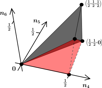

From the left side we can infer again that the GPCs are more restrictive than Pauli’s exclusion principle constraints since the respective polytope is a proper subset of the Pauli simplex (given by the polytope together with an extension shown in red). On the right side, the geometric picture as introduced in Section 2.3 is presented. The vector of NONs follows as the center of mass of masses located at the positions , the vertices of the Pauli hypercube. Their restrictions to the -subspace are given by (recall Eq. (11))
In case of non-degenerate NONs, only the configurations may contribute in the self-consistent expansion (8) according to (30) whose unordered spectra lie on the hyperplane corresponding to pinning (shown in blue). The same is still true in case of degeneracies or . For a degeneracy (i.e. ) and a generic choice of the natural orbitals in the subspace also the configurations whose vectors lie on the light blue hyperplane may contribute. This latter hyperplane is given by the swapping of the blue hyperplane. Yet, according to (33) there exists at least one basis of natural orbitals with respect to which the weights on the light blue hyperplane are transformed away and would lie solely on the blue hyperplane.
The analysis of the Borland-Dennis setting suggests the following implications of pinning by a GPC in a general setting : In case of non-degenerate NONs there is no ambiguity since the natural orbitals are unique and only those configurations may contribute to whose unordered spectra (recall Eq. (12)) lie on the respective hyperplane corresponding to pinning, . In case of degenerate NONs there exist at least one basis of natural orbitals with respect to which the original selection rule for non-degenerate NONs applies.
Although those main results of our work (see Theorems 6, 10 and Corollaries 7, 11 below) could be presented for both cases of non-degenerate and degenerate NONs together, we split them. This has the advantage that at least the results for non-degenerate NONs can be stated in a less technical form, namely not involving the ambiguity of natural orbital bases. For the proofs of various results we refer the reader to Part II.
4.4 Implications of non-degenerate pinned occupation numbers
In case of non-degenerate NONs the structural implications of pinning can be stated as
Theorem 6 (Pinning of non-degenerate NONs).
Let be an -fermion quantum state whose non-degenerate NONs saturate a GPC, and denote the family of ’s unique natural orbitals by . Then, lies in the zero-eigenspace of the respective -operator (recall Definition 1), i.e.
| (61) |
It is worth noticing that Theorem 6 applies to various saturated GPC simultaneously.
Theorem 6 implies immediate structural simplifications for the state which are particularly well-pronounced in the self-consistent expansion (8) as already illustrated above:
Corollary 7 (Selection rule for non-degenerate NONs).
We present an example which illustrates Theorem 6 and the corresponding selection rule, Corollary 7:
Example 8.
We consider non-degenerate NONs in the setting that are saturating one of the GPCs, namely
| (63) |
According to Theorem 6 any corresponding quantum state has to lie in the zero-eigenspace of the respective -operator,
| (64) |
Corollary 7 then identifies all configurations which may contribute to the self-consistent expansion of , namely . This reduction of configurations to just highlights the remarkable implications of pinning as an effect in the one-particle picture on the structure of the corresponding many-fermion quantum state.
4.5 Implications of degenerate pinned occupation numbers
Based on the analysis of pinning by degenerate NONs in the Borland-Dennis setting (Section 4.3) one may expect the following generalization of Theorem 6 to degenerate NONs:
Conjecture 9.
Let be an -fermion quantum state whose degenerate NONs saturate some (possibly several) GPCs. Then, there exists an orthonormal basis of natural orbitals such that lies in the zero-eigenspace of the respective -operators of various saturated GPCs (recall Definition 1), i.e.
| (65) |
There are actually a number of reasons (highlighted in Part II which presents various mathematical proofs) why the generalization of Theorem 6 to non-degenerate NONs and its proof are quite involved.
In the following we present a weaker extension of Theorem 6 to degenerate NONs. It refers to the saturation of exactly one GPC. Its proof requires in addition the validity of a technical assumption (presented as Assumption 13 in Part II) which we could verify for all GPCs known so far. Hence, there is little doubt that the assumption is always valid and the corresponding addition to the following theorem might be unnecessary.
Theorem 10 (Pinning of degenerate NONs).
Let be an -fermion quantum state whose degenerate NONs saturate exactly one GPC, and assume that the technical Assumption 13 from Part II is met. Then, there exists an orthonormal basis of natural orbitals such that lies in the zero-eigenspace of the respective -operator (recall Definition 1), i.e.
| (66) |
Despite the ambiguity of the natural orbital basis it is worth recalling that the natural orbitals are still referring to the non-increasingly ordered NONs (see also (4)).
In complete analogy to Theorem 6 and Corollary 7, Theorem 10 implies immediately a corresponding selection rule identifying all configurations which may contribute to in case of pinning:
Corollary 11 (Selection rule for degenerate NONs).
Let whose degenerate NONs saturate exactly one GPC, and assume that the technical Assumption 13 from Part II is met. Then, there exists an orthonormal basis of natural orbitals such that only configurations may contribute to the self-consistent expansion (8) of whose unordered spectra (recall Eq. (11)) lie on the the hyperplane , i.e.
| (67) |
4.6 Converse selection rule: Rationalizing pinning-based multiconfigurational ansatzes
The remarkable implications of pinning as an effect in the one-fermion picture on the structure of the -fermion quantum state offers an alternative characterization of some existing variational post-Hartree-Fock ansatzes and suggests additional new ones: Each face of the polytope , as characterized by a certain number of saturated Pauli constraints, generalized Pauli constraints and ordering constraints , defines a state manifold of quantum states. These are exactly those states whose NONs map to the face ,
| (68) |
Minimizing the energy expectation value of a given Hamiltonian of a system of interacting fermions over then defines a variational scheme associated with the face with a corresponding variational energy
| (69) |
From a qualitative point of view, one can say that the higher dimensional the face , the higher dimensional the corresponding state manifold and thus the more computationally demanding the respective ansatz. Some well-known examples for such polytope face-associated variational schemes are the Complete Active Space Self-Consistent Field (CASSCF) ansatzes (see, e.g., Refs. [5, 6, 7, 8]). Indeed, according to Theorem 2 they can be characterized by the saturation of a certain number of Pauli exclusion principle constraints. Our main results, Theorems 6, 10 and the respective selection rules, Corollaries 7, 11, highlight that even more elaborated variational ansatzes can be introduced by referring not only to the saturation of Pauli constraints but to extremal one-fermion information in general, i.e., pinned NONs. The motivation for proposing such generalizations of CASSCF ansatzes is twofold. On the one hand, the study of smaller atoms [45] has reveled that the GPCs have an additional significance for ground states beyond the one of the Pauli exclusion principle constraints, as quantified by the -parameter [14]. On the other hand, not all configurations within a complete active space are relevant and it would be preferable to identify only the most significant ones. The gain in computational time could be used to increase the basis set size, allowing one to recover more of the dynamic correlation.
A comment is in order concerning the practical implementation of such variational schemes. After having fixed , i.e. the corresponding family of contributing configurations , one would minimize both the respective expansion coefficients and the involved natural orbitals . Such variational approaches are known in quantum chemistry as Multiconfiguration Self-Consistent Field (MCSCF)-ansatzes (see, e.g., the textbook [57]). Yet, the stringent use of pinning-based variational ansatzes in the form (74) would be quite challenging and not particularly efficient. This is due to the fact that the selection rule 7 defines by referring to the self-consistent expansion (8), i.e. rather involved self-consistency conditions on the expansion coefficients would need to be imposed. From a converse point of view, an arbitrary superposition of all allowed configurations is typically not self-consistent. Hence, its relation to the face seems to be rather loose, since its vector of non-increasingly ordered NONs lies actually in the interior of the polytope rather than on the face . To illustrate this, let us revisit Example 8. We pick a random (real-valued) superposition of the allowed configurations listed in Example 8: . The corresponding vector of decreasingly-ordered NONs follows as
| (70) | |||||
For the GPC (63) at hand, one finds , i.e. lies far away from the polytope facet defined by . This is actually quite different for the vector obtained by permuting the NONs according to some specific permutation . Of course, does not lie in the polytope anymore since its entries are not properly ordered. Yet, by extending the face of to a hyperplane in the space of all occupation number vectors (including the ones which are not decreasingly ordered), turns out to lie on that hyperplane, . This is rather astonishing in particular since the one-particle reduced density matrices of such arbitrary superpositions are not diagonal in the original reference basis anymore. For instance, one finds for the superposition above . This surprising example has actually a deep origin:
Theorem 12 (Converse selection rule).
Let be a face of the polytope of the setting defined by the saturation of a specific family of GPCs . For an orthonormal basis of we define
| (71) |
i.e. the vector space of all superpositions of configurations fulfilling the selection rule 7 with respect to the basis for all GPCs with . Then, for any there exists a basis of (possibly wrongly ordered) natural orbitals of such that all configurations also fulfil the selection rules for all . In particular, the corresponding vector of (possibly wrongly ordered) NONs saturates for all , i.e. lies on the hyperplane obtained by extending the face to non-decreasingly ordered occupation number vectors.
To illustrate the first part of this theorem we revisit Example 8. Let be some orthonormal basis for and consider the GPC from Example 8. The corresponding linear space follows as (where denotes the face defined by )
| (72) | |||||
Let , i.e. is a linear combination of the nine specific configuration states shown in (72). As already explained above, the corresponding one-particle reduced density matrix of is in general not diagonal with respect to , i.e. its natural orbital basis is different than . Naively one may thus expect that the self-consistent natural orbital expansion (8) of would involve all 56 configurations. Yet, the first part of Theorem 12 states that this is not the case. In particular, there exists a permutation of ’s ordered natural orbitals yielding with the effect that only those contribute to which fulfil the selection rule .
The converse selection rule 12 establishes a more flexible relation between quantum states and polytope faces since it does not refer to the self-consistent expansion (8) anymore. In particular, it therefore provides a solid foundation for more effective pinning-based MCSCF ansatzes minimizing the energy expectation value of a Hamiltonian over all states in
| (73) |
Such ansatzes are indeed MCSCF ansatzes in a strict sense: In a first step, one identifies (via the choice of a face ) a specific set of configurations contributing to . Then, in a second step one minimizes the energy expectation value with respect to various expansion coefficients (without any additional constraints on them) and all possible orbital choices . The corresponding variational energy
| (74) |
is at least as good as the original one () and the computational effort is significantly reduced by omitting the quadratic self-consistency conditions required in the characterization of .
It will be one of the future challenging to implement and test such pinning-based MCSCF ansatzes (for a proof of concept see [48]). In particular, one needs to develop a systematic procedure for identifying the appropriate polytope faces , e.g., in the form of a renormalization group-inspired scheme which exploits the inclusion hierarchy of faces of different dimensionalities [58].
4.7 Presence of pinning reveals symmetries of quantum states
According to Theorem 6 and its generalization including the case of degenerate NONs, Theorem 10, pinning implies that the -fermion quantum state lies in the zero-eigenspace of the corresponding natural orbital induced operator . This means nothing else than that is the generator of a continuous symmetry of ,
| (75) |
This symmetry could be a hidden symmetry of the state itself or a symmetry of the Hamiltonian.
We present a prominent example for a pinned quantum state. For the Hubbard model with three sites and three electrons the ground state was shown to exhibit pinning [41]. In the self-consistent expansion (8) it takes the form (30). The corresponding natural orbitals are given by the following spin-momentum states ()
| (76) |
The corresponding natural orbital induced operator thus reads
| (77) |
The presence of pinning in the Hubbard trimer reflects the system’s -symmetry, generated by the total spin along the -axis. It would be interesting to explore the meaning of those symmetry operators, e.g. for the harmonic trap systems shown to exhibit (approximate) pinning [32].
5 Summary and conclusion
The concept of active spaces simplifies the description of interacting quantum many-body systems by restricting to a neighbourhood of active orbitals around the Fermi level. The respective -fermion wavefunction ansatzes can be characterized by the saturation of a certain number of Pauli constraints , identifying the occupied core orbitals () and the inactive virtual orbitals (). By referring to the generalized Pauli constraints, completing Pauli’s original exclusion principle, we have provided a natural generalization of the concept of active spaces: We have explained and comprehensively illustrated that the saturation of any one-body -representability condition defines a distinctive space of active electron configurations contributing to the wave function ansatz (see Theorems 6,10,12 and the selection rules 7,11). In contrast to the traditional complete active spaces defined through the saturation of Pauli’s exclusion principle constraints, the use of such generalized active spaces does not necessarily mean to neglect dynamical correlations since more orbitals may contribute while the number of contributing configurations is still restricted. In particular, the choice of appropriate generalized active spaces would identify in an efficient and systematic way the significant electron configurations (rather than taking all of them into account as in complete active space self-consistent field (CASSCF)-ansatzes). The present Part I therefore provides the theoretical foundation for possible wavefuntion based methods exploiting the fruitful mathematical structure underlying the generalized Pauli constraints. From a practical point of view, to achieve the full potential of our more systematic multiconfigurational approach, more effort needs to be spent on the mathematical side to calculate the generalized Pauli constraints for larger system sizes.
Moreover, according to Theorems 6, 10, pinning as an effect in the one-particle picture reveals the presence of symmetries. Those could be global symmetries of the underlying Hamiltonian (as, e.g., for Hubbard model clusters) or symmetries of just the quantum state at hand. Consequently, the successful search of possible (quasi)pinning in quantum systems could reveal and characterize possible ground state symmetries.
Acknowledgments
We thank D.Gross for helpful discussions. We also acknowledge financial support from the UK Engineering and Physical Sciences Research Council (Grant EP/P007155/1) and the German Research Foundation (Grant SCHI 1476/1-1) (CS), the National Science Centre, Poland under the grant SONATA BIS: 2015/18/E/ST1/00200 (AS),
the Excellence Initiative of the German Federal and State Governments (Grants ZUK 43 & 81) (AL).
References
- [1] A. J. Coleman. Structure of fermion density matrices. Rev. Mod. Phys., 35:668, Jul 1963.
- [2] A. J. Coleman and V. I. Yukalov. Reduced Density Matrices: Coulson’s Challenge. Springer, New York, 2000.
- [3] T. L. Gilbert. Hohenberg-Kohn theorem for nonlocal external potentials. Phys. Rev. B, 12:2111–2120, 1975.
- [4] K. Pernal and K. J. H. Giesbertz. Reduced Density Matrix Functional Theory (RDMFT) and Linear Response Time-Dependent RDMFT (TD-RDMFT), page 125. Springer International Publishing, Cham, 2016.
- [5] P. Siegbahn, A. Heiberg, B. Roos, and B. Levy. A comparison of the super-CI and the Newton-Raphson scheme in the complete active space SCF method. Phys. Scr., 21(3-4):323, 1980.
- [6] B. Roos, P. Taylor, and P. Siegbahn. A complete active space SCF method (CASSCF) using a density matrix formulated super-CI approach. Chem. Phys., 48(2):157 – 173, 1980.
- [7] P. Siegbahn, J. Almlöf, A. Heiberg, and B. Roos. The complete active space scf (CASSCF) method in a Newton-Raphson formulation with application to the HNO molecule. J. Chem. Phys., 74(4):2384–2396, 1981.
- [8] J. Olsen. The CASSCF method: A perspective and commentary. Int. J. Quant. Chem., 111(13):3267–3272, 2011.
- [9] R. E. Borland and K. Dennis. The conditions on the one-matrix for three-body fermion wavefunctions with one-rank equal to six. J. Phys. B, 5(1):7, 1972.
- [10] A. Klyachko. Quantum marginal problem and representations of the symmetric group. arXiv:0409113, 2004.
- [11] M. Altunbulak and A. Klyachko. The Pauli principle revisited. Commun. Math. Phys., 282:287–322, 2008.
- [12] M. Altunbulak. The Pauli principle, representation theory, and geometry of flag varieties. PhD thesis, Bilkent University, 2008.
- [13] C. Schilling. Quasipinning and its relevance for -fermion quantum states. Phys. Rev. A, 91:022105, 2015.
- [14] F. Tennie, V. Vedral, and C. Schilling. Influence of the fermionic exchange symmetry beyond Pauli’s exclusion principle. Phys. Rev. A, 95:022336, Feb 2017.
- [15] P.-O. Löwdin. Quantum theory of many-particle systems. I. physical interpretations by means of density matrices, natural spin-orbitals, and convergence problems in the method of configurational interaction. Phys. Rev., 97:1474, 1955.
- [16] E. R. Davidson. Properties and uses of natural orbitals. Rev. Mod. Phys., 44:451, 1972.
- [17] P.-O. Löwdin and H. Shull. Natural orbitals in the quantum theory of two-electron systems. Phys. Rev., 101:1730, 1956.
- [18] W. Pauli. Über den Zusammenhang des Abschlusses der Elektronengruppen im Atom mit der Komplexstruktur der Spektren. Z. Phys., 31:765–783, 1925.
- [19] F. J. Dyson and A. Lenard. Stability of matter. i. J. Math. Phys., 8(3):423–434, 1967.
- [20] E.H. Lieb. The stability of matter. Rev. Mod. Phys., 48:553–569, 1976.
- [21] A. Klyachko. Quantum marginal problem and N-representability. J. Phys. Conf. Ser., 36(1):72, 2006.
- [22] F. Tennie, D. Ebler, V. Vedral, and C. Schilling. Pinning of fermionic occupation numbers: General concepts and one spatial dimension. Phys. Rev. A, 93:042126, 2016.
- [23] D.W. Smith. N-representability problem for fermion density matrices. ii. the first-order density matrix with n even. Phys. Rev., 147:896, 1966.
- [24] M. B. Ruskai. Connecting N-representability to Weyl’s problem: the one-particle density matrix for N = 3 and R = 6. J. Phys. A, 40(45):F961, 2007.
- [25] T. Macia̧żek and V. Tsanov. Quantum marginals from pure doubly excited states. J. Phys. A, 50:465304, 2017.
- [26] R. J. Bell, R. E. Borland, and K. Dennis. The n+2 spin-orbital approximation to the n-body antisymmetric wave function. J. Phys. B, 3(8):1047, aug 1970.
- [27] C. Schilling, D. Gross, and M. Christandl. Pinning of fermionic occupation numbers. Phys. Rev. Lett., 110:040404, 2013.
- [28] D. Ebler. Pinning analysis for -harmonium. Semester thesis, ETH Zurich, 2013.
- [29] C. Schilling. Quantum marginal problem and its physical relevance. PhD thesis, ETH-Zürich, 2014.
- [30] F. Tennie, V. Vedral, and C. Schilling. Pinning of fermionic occupation numbers: Higher spatial dimensions and spin. Phys. Rev. A, 94:012120, 2016.
- [31] F. Tennie. Influence of the exchange symmetry beyond the exclusion principle. PhD thesis, University of Oxford, 2017.
- [32] Ö. Legeza and C. Schilling. Role of the pair potential for the saturation of generalized Pauli constraints. Phys. Rev. A, 97:052105, May 2018.
- [33] A. Klyachko. The Pauli exclusion principle and beyond. arXiv:0904.2009, 2009.
- [34] C. L. Benavides-Riveros, J. M. Gracia-Bondía, and M. Springborg. Quasipinning and entanglement in the lithium isoelectronic series. Phys. Rev. A, 88:022508, 2013.
- [35] A. Klyachko. The Pauli principle and magnetism. arXiv:1311.5999, 2013.
- [36] R. Chakraborty and D.A. Mazziotti. Generalized Pauli conditions on the spectra of one-electron reduced density matrices of atoms and molecules. Phys. Rev. A, 89:042505, 2014.
- [37] R. Chakraborty and D.A. Mazziotti. Sufficient condition for the openness of a many-electron quantum system from the violation of a generalized Pauli exclusion principle. Phys. Rev. A, 91:010101, 2015.
- [38] C. L. Benavides-Riveros and M. Springborg. Quasipinning and selection rules for excitations in atoms and molecules. Phys. Rev. A, 92:012512, 2015.
- [39] R. Chakraborty and D. A. Mazziotti. Structure of the one-electron reduced density matrix from the generalized Pauli exclusion principle. Int. J. Quant. Chem., 115(19):1305–1310, 2015.
- [40] A. Lopes. Pure univariate quantum marginals and electronic transport properties of geometrically frustrated systems. PhD thesis, University of Freiburg, 2015.
- [41] C. Schilling. Hubbard model: Pinning of occupation numbers and role of symmetries. Phys. Rev. B, 92:155149, 2015.
- [42] C. L. Benavides-Riveros. Disentangling the marginal problem in quantum chemistry. PhD thesis, Universidad de Zaragoza, 2015.
- [43] R. Chakraborty and D. A. Mazziotti. Role of the generalized Pauli constraints in the quantum chemistry of excited states. Int. J. Quant. Chem., 116, 2016.
- [44] R. Chakraborty and D.A. Mazziotti. Noise-assisted energy transfer from the dilation of the set of one-electron reduced density matrices. J. Chem. Phys., 146(18):184101, 2017.
- [45] C. Schilling, M. Altunbulak, S. Knecht, A. Lopes, J. D. Whitfield, M. Christandl, D. Gross, and M. Reiher. Generalized Pauli constraints in small atoms. Phys. Rev. A, 97:052503, May 2018.
- [46] C. Schilling. The quantum marginal problem. In P. Exner, W. König, and H. Neidhardt, editors, Mathematical Results in Quantum Mechanics, chapter 10, pages 165–176. World Scientific, 2014.
- [47] C. Schilling, C. L. Benavides-Riveros, and P. Vrana. Reconstructing quantum states from single-party information. Phys. Rev. A, 96:052312, 2017.
- [48] C. L. Benavides-Riveros and C. Schilling. Natural extension of Hartree-Fock through extremal 1-fermion information: Overview and application to the Lithium atom. Z. Phys. Chem., 230, 2016.
- [49] R. Chakraborty and D. A. Mazziotti. Sparsity of the wavefunction from the generalized Pauli exclusion principle. J. Chem. Phys., 148(5):054106, 2018.
- [50] C. L. Benavides-Riveros and M. A. L. Marques. Static correlated functionals for reduced density matrix functional theory. Eur. Phys. J. B, 91(6):133, 2018.
- [51] J.-N. Boyn and D. A. Mazziotti. Sparse non-orthogonal wave function expansions from the extension of the generalized Pauli constraints to the two-electron reduced density matrix. J. Chem. Phys., 150(14):144102, 2019.
- [52] I. Theophilou, N.N. Lathiotakis, M. Marques, and N. Helbig. Generalized Pauli constraints in reduced density matrix functional theory. J. Chem. Phys., 142(15), 2015.
- [53] C. Schilling. Communication: Relating the pure and ensemble density matrix functional. J. Chem. Phys., 149(23):231102, 2018.
- [54] I. Theophilou, N. N. Lathiotakis, and N. Helbig. Conditions for describing triplet states in reduced density matrix functional theory. J. Chem. Theory Comput., 12(6):2668, 2016.
- [55] I. Theophilou, N. N. Lathiotakis, and N. Helbig. Structure of the first order reduced density matrix in three electron systems: A generalized Pauli constraints assisted study. J. Chem. Phys., 148(11):114108, 2018.
- [56] C. Schilling and R. Schilling. Diverging exchange force and form of the exact density matrix functional. Phys. Rev. Lett., 122:013001, Jan 2019.
- [57] T. Helgaker, P. Jørgensen, and O. Jeppe. Molecular Electronic-Structure Theory. John Wiley, 2012.
- [58] C. Schilling. unpublished.