Fundamental energy requirement of reversible quantum operations

Here we consider the fundamental energy requirement for implementing quantum operations. Such requirement consists of at least two different contributions, which are consequences of the second law of thermodynamics and of energy conservation in quantum mechanics, respectively. The fact that the second law of thermodynamics has implications for the energy cost of computation is known as Landauer’s principle Landauer 1961. It asserts that any physical device that carries out a logically irreversible operation dissipates a certain minimum amount of energy as heat, and that this amount is proportional to the degree of irreversibility (which may be quantified in terms of entropic quantities, see Sagawa and Ueda 2009; Reeb and Wolf 2014; Faist et al. 2015; Faist and Renner 2018).

In this work we are concerned with the second fundamental contribution to the energy bill. This contribution can be regarded as a consequence of energy conservation, when applied to coherent transitions across states of different energy. If a process is executed on a system with non-degenerate energy levels then energy must be temporarily borrowed from a battery. For general quantum processes, this borrowing may occur in a superposition, i.e., the system’s quantum state may consist of one branch in which energy has flown from the battery and another one in which energy has flown into the battery. To ensure that this does not lead to decoherence, the corresponding energy states of the battery must be indistinguishable. This, in turn, is only possible if the battery is large enough. Determining the corresponding energy requirement is exactly the topic of this work.

Previous approaches to quantify the energy requirement are based on the Wigner-Araki-Yanase (WAY) theorem Wigner 1952; Araki and Yanase 1960, which states that any conservation law limits the accuracy with which quantities that do not commute with the conserved quantity can be measured. The theorem implies a bound on the variance of the energy in the initial state of the battery required to implement an operation Ozawa 2002; Ozawa 2003; Gea-Banacloche and Ozawa 2006; Karasawa and Ozawa 2007; Karasawa et al. 2009; Tajima et al. 2018. However, the variance does not in general provide a good bound on the size of the battery, nor on the average energy that needs to be initially stored in it. As a simple example, consider a system with $d$ equally spaced energy levels $\{E_{0},\dots,E_{d-1}\}$. A pure state in the superposition of energy eigenstates corresponding to $E_{0}$ and $E_{d-1}$ with amplitudes $\smash{\sqrt{1-1/d}}$ and $\smash{\sqrt{1/d}}$, respectively, has average energy (measured relative to $E_{0}=0$) less than $E_{1}$ and large energy variance that grows as $d$. On the other hand, even if the variance is fixed the energy can still take an arbitrarily large value.

Here we instead take a general resource-theoretic approach. Let $M$ be a function that quantifies the value of the different possible states of a system with respect to a resource. For example, $M(\rho)$ may be the average energy of the system when it is in state $\rho$. Furthermore, for a reversible operation $G$ on the system, we denote by $M(G)$ the maximum increase of the function $M$ when evaluated on an input state and on the corresponding output state produced by $G$. Hence, in the case where the considered resource is energy, $M(G)$ quantifies by how much the system’s energy can grow when executing $G$. Assume now that we want to implement $G$ up to a precision $\epsilon$ (which we quantify in terms of the worst-case infidelity, defined below). The implementation should consist of a device that can merely carry out free operations, i.e., operations that cannot generate the resource. Such an implementation must necessarily use a battery, as illustrated in Fig. 1. Then the following general assertion can be made.

This theorem, whose proof we will sketch in the first section below, yields in particular a lower bound on the energy requirement for implementing a reversible operation $G$. Specifically, in the second section, we show that the average energy content $\langle H_{\rm B}\rangle$ of the battery supplying energy to the processor must be at least

where $\|H_{\rm S}\|$ is the operator norm of the system’s Hamiltonian, $\lambda_{\max}$ ($\lambda_{\min}$) denotes the maximal (minimal) eigenvalue, and $\Delta_{G}H_{\rm S}=G^{\dagger}H_{\rm S}G-H_{\rm S}$ is the change of the system’s Hamiltonian induced by the action of the gate $G$. We have assumed, without loss of generality, that the minimum energy is zero for both the system and the battery, and thus $\|H_{\rm S}\|$ is equal to the maximum energy of the system. The bound (1) states that the average energy of the battery should be above the ground state energy by an amount determined by the energy change operator $\Delta_{G}H_{\rm S}$, the system’s energy scale $\|H_{\rm S}\|$, and the error $\epsilon$.

While the bound (1) depends on the particular operation $G$, by maximising over all such reversible operations we obtain a bound on the energy requirement of a universal quantum processor operating on a system $S\rm$ with a given Hamiltonian $H_{\rm S}$,

This bound is tight up to a constant factor. More precisely, assuming that the system has equally spaced energy levels, we show by an explicit construction, described in the third section below, that

Taking together these two bounds, we have thus established that the fundamental energy requirement for operating on $\rm S$ grows as $\|H_{\rm S}\|/\sqrt{\epsilon}$. Note that if the system’s Hamiltonian is fully degenerate, i.e., $\|H_{\rm S}\|=0$ then energy conversation does not imply an energy requirement. Besides the average energy, we show that the energy spread of the battery is lower bounded by $\|H_{\rm S}\|/\sqrt{\epsilon}$, and the tightness of the bound can again be achieved with the construction that led to (3).

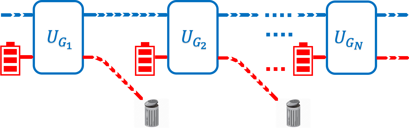
Finally, we determine how the energy requirement of a quantum circuit depends on its complexity. Previous works considered implementations of quantum circuits where each gate is powered by an independent battery Ozawa 2002; Gea-Banacloche and Ozawa 2006 (see Fig. 2). The energy requirement then obviously grows linearly with the number of non-conservative gates, making complex computations energetically demanding. In contrast, we show that the energy requirement of quantum circuits is independent of their complexity. For this we consider an implementation that uses a single battery to power all gates in the circuit (see Fig. 2). It turns out that energy can be recycled from one gate to the next, and that the energy requirement for a sequence of gates is exactly equal to the energy requirement of the overall gate resulting from their composition. Hence, the energy requirement depends only on the size of the computational register, but not on the time complexity of the computation. For quantum computations with classical inputs and outputs, such as Shor’s algorithm, we further show that our implementation is exact and the energy requirement is just the energy needed to write down the output of the computation. This may be regarded as the quantum analogue of a classical result by Fredkin and Toffoli Fredkin and Toffoli 1982, who studied the fundamental energy constraints that the classical laws of physics impose on computation.

To quantify how well the operation $\mathcal{E}_{G}$ approximates a desired gate $G$ we use the worst-case fidelity $F_{\rm wc}$ between the output of $G$ and $\mathcal{E}_{G}$ for any input, which may also be correlated to an external reference system ${\rm R}$. That is, explicitly,

with $\Psi:=|\Psi\rangle\langle\Psi|$, $\mathcal{G}(\cdot)=G\cdot G^{\dagger}$, and $\mathcal{I}_{\rm R}$ denoting the identity map on $L(\mathcal{H}_{\rm R})$, the space of linear operators on $\mathcal{H}_{\rm R}$. We say that an implementation has error $\epsilon$ if $F_{\rm wc}=1-\epsilon$. The use of this error measure is justified by the fact that the resource requirements, in the case of energy as discussed in the introduction, can be bounded tightly in terms of $\epsilon$ (up to a constant). We also note that the fidelity is easy to evaluate and widely used to quantify the quality of gates in quantum computation. Moreover, it may be related to other measures of distance, e.g., the diamond norm Kitaev 1997 (see dia for a definition) via the inequalities $1-\sqrt{F_{\rm wc}}\leq\frac{1}{2}\|\mathcal{E}_{G}-\mathcal{G}\|_{\diamond}\leq\sqrt{1-F_{\rm wc}}$. In Appendix D, we show that the dependence of the energy requirement on the diamond norm also scales as $1/\sqrt{\epsilon}$, up to a factor that may however depend on the system’s dimension.

Theorem 1 is a general resource-theoretic statement, which merely depends on general properties of the measure $M$ used to quantify resourcefulness. Specifically, for any given system, $M$ is a function of the density operator of that system such that the following holds:

1. 1.

   Monotonicity. $M$ is non-increasing under free operations and partial trace.

2. 2.

   Additivity on product states. $M(\rho\otimes\sigma)=M(\rho)+M(\sigma)$.

3. 3.

   Regularity. There exists a constant $c\in\mathbb{R}$ and, for any system $\rm S$, a Lipschitz constant $K_{\rm S}\geq 0$, such that $|M(\rho)-M(\sigma)|\leq K_{\rm S}\,\|\rho-\sigma\|_{1}+c$ for any states $\rho$ and $\sigma$ of system $\rm S$, and such that $K_{\rm S}$ is subadditive, i.e., $K_{\rm AB}\leq K_{\rm A}+K_{\rm B}$ for any systems $\rm A$ and $\rm B$.

With these definitions in place, we can now proceed to the proof of Theorem 1. Let $\mathcal{V}_{G}(\cdot):=\mathcal{U}_{G}(\cdot\otimes\beta)$ with $\mathcal{U}_{G}(\cdot)=U_{G}\cdot U_{G}^{\dagger}$ be the evolution defined in (4), but before tracing out the battery $\rm B$. Using techniques from Kretschmann et al. 2008a; Chiribella et al. 2013; Gutoski et al. 2017 we show (see Appendix A) that the channel $\mathcal{V}_{G}$ is close to $\mathcal{G}\otimes\beta^{\prime}$, where $\beta^{\prime}$ is a suitable battery state 2fo. Due to its additivity property, it is useful to measure this closeness in terms of the diamond norm $\|\cdot\|_{\diamond}$ dia

But this means that approximately there is no entanglement between the system and the battery after the evolution, and the battery ends up in a state close to $\beta^{\prime}$. Conversely, the state $\beta^{\prime}$ may be used to approximately implement the inverse gate $G^{\dagger}$, using the gate $U_{G}^{\dagger}$, i.e.,

with $\mathcal{V}^{\prime}_{G}(\cdot):=\mathcal{U}_{G}^{-1}(\cdot\otimes\beta^{\prime})$.

According to (6) and (7) we may thus implement the gate $G^{\dagger}$ after gate $G$, thereby returning the ancilla approximately to its initial state. Repeating this procedure $m$ (for any $m\in\mathbb{N}$) times, i.e., composing $m$ implementations of $G$ and of $G^{\dagger}$ in alternating order as illustrated in Fig. 3, we still approximate each of them within an error bounded by $4m\sqrt{\epsilon}$. Note that the circuit in the lower half of the figure increases the resource value $M$ by virtue of $G$ and $G^{\dagger}$. To approximate this increase of resource, the circuit in the upper half of the picture must use the battery, because all the other operations in the circuit are free and therefore resource non-generating. Hence, the amount of resource generated by $m$ uses of $G$ and $G^{\dagger}$, i.e., $m$ times $M(G)+M(G^{{\dagger}})$, must be matched by the battery. Evaluating this amount leads to the bound stated in Theorem 1.

In a similar way we can also derive a lower bound on the required total capacity $\|H_{\rm B}\|$ of the battery. For this we first apply Theorem 1 to the resource function $M^{\prime}(\rho):=\operatorname{Tr}\rho(\|H\|\cdot I-H)$ to obtain the bound

Taking the worst case $G$, which satisfies $\lambda_{\max}(\Delta_{G}H_{\rm S})=-\lambda_{\min}(\Delta_{G}H_{\rm S})=\|H_{\rm S}\|$, and combining this with bound (1), we find a bound on the maximum energy (or the capacity) of the battery,

This and (2) are lower bounds on the energy requirement of a universal processor, able to implement arbitrary gates on system $\rm S$ with error $\epsilon$ or less. While (2) quantifies the energy requirement in terms of the average energy that a battery must contain, (9) refers to the battery’s total capacity.

Theorem 1 also provides bounds on other types of resources, such as coherence Baumgratz et al. 2014; Winter and Yang 2016; Marvian and Spekkens 2016; Streltsov et al. 2017. A concrete example is the relative entropy of coherence Baumgratz et al. 2014 $C(\rho):=S(\rho_{\rm diag})-S(\rho)$, with $S$ denoting the von Neumann entropy and $\rho_{\rm diag}$ the diagonal part of $\rho$ in the energy eigenbasis. Here the theorem yields the bound (see Appendix B)

on the initial coherence that the battery must provide, where $d_{\rm S}$ is the dimension of the system on which $G$ acts, and $C({G})$ is the amount of coherence generated by the gate $G$. For gates like the generalized Hadamard gate this quantity can be as large as $\log d_{\rm S}$. Therefore, the minimum amount of coherence required to operate a universal quantum processor scales like $\log d_{\rm S}/\sqrt{\epsilon}$.

We have shown that the requirement for energy and coherence both follow an $1/\sqrt{\epsilon}$ scaling. The same scaling characterises also the standard deviation of the energy, as observed in previous works Ozawa 2002; Ozawa 2003; Gea-Banacloche and Ozawa 2006; Karasawa and Ozawa 2007; Karasawa et al. 2009; Tajima et al. 2018.

The implementation uses a battery with equally spaced energy levels with spacing $\hbar\omega$, ranging from $0$ to $\|H_{\rm B}\|=R\|H_{\rm S}\|$, where $R$ is an integer, assumed to be larger than 2 for later convenience. At the beginning, the battery is initialized in a superposition of energy eigenstates with sine-shaped amplitudes Bužek et al. 1999

where the summation runs in steps of $\hbar\omega$, and $L=({R-2})\|H_{\rm S}\|/(\hbar\omega)+2$. Note that the lowest and highest energy levels are unoccupied. This allows the battery to both supply and absorb energy from the system.

For the interaction between the system and the battery we adopt a construction from Refs. Skrzypczyk et al. 2013; Åberg 2014; Navascués and Popescu 2014, suitably adapted to unitary gates on finite-dimensional systems. Denote by $E_{\rm S,x}$ the energy of $|\psi_{x}\rangle$. For a given value $E$ of the total energy, and for every $x$ satisfying the condition

we define the eigenstates

Then, we denote by $\mathsf{E}_{\rm ok}$ the set of values of the total energy such that condition (12) is satisfied for every $x=1,\dots,d_{\rm S}$, or equivalently, the set of values $E$ satisfying the condition $\|H_{\rm S}\|\leq E\leq\|H_{\rm B}\|$. For every $E\in\mathsf{E}_{\rm ok}$, define the partial isometry

which acts as the unitary gate $G$ in the eigenspace with total energy $E$. To make the computation reversible on the whole system $\rm SB$, we set $U_{G}$ to be the unitary gate

where $P_{E}$ is the projector on the subspace with total energy $E$.

In Appendix C we show that the worst case fidelity of the above implementation is lower bounded as

and therefore the energy requirement is upper bounded as

In the worst case over all possible gates, one has $(\lambda_{\max}-\lambda_{\min})(\Delta_{G}H_{\rm S})=2\|H_{\rm S}\|$, matching the lower bound (2) up to a constant factor of $4\pi$.

The error $\epsilon$ depends on the parameter $R$ that characterizes the battery state (11). Observing that the energy of the sine state is $\langle H_{\rm B}\rangle=R\|H_{\rm S}\|/2$, we obtain the dependency $R\approx\pi(\lambda_{\max}-\lambda_{\min})(\Delta_{G}H_{\rm S})/(2\sqrt{\epsilon}\|H_{\rm S}\|)$. Therefore, the battery capacity of this implementation is $\|H_{\rm B}\|=R\|H_{\rm S}\|\approx\pi(\lambda_{\max}-\lambda_{\min})(\Delta_{G}H_{\rm S})/(2\sqrt{\epsilon})$. Taking the worst-case $G$, the capacity of the battery is approximately

matching the lower bound (9) up to a constant of $4\pi$.

We now show that, in fact, quantum computation can be implemented with an amount of energy that is independent of the circuit depth. To do so, we propose a scheme of computation where energy is recycled from one computational step to the next. The computation is performed on $n$ identical qubits, each with Hamiltonian $H_{\rm S}^{(1)}$ and energy gap $\|H_{\rm S}^{(1)}\|=\hbar\omega$, and uses a single battery of capacity $C_{\rm B}=Rn\|H^{(1)}_{\rm S}\|$, where $R$ is an integer depending on the desired level of accuracy. For an elementary gate $G$ acting on a subset of $k$ qubits, we let the battery and the $k$ qubits interact through the energy-preserving gate $U_{G}$ in (15). The energy subspaces on which the gate $U_{G}$ acts non-trivially correspond to the energy values $\mathsf{E}_{\rm ok}^{(k)}=\{E\,|~k\,\|H_{\rm S}^{(1)}\|\leq E\leq\|H_{\rm B}\|\}$. Now, consider the total energy of the $n$ qubits and the battery. For every two gates $G_{1}$ and $G_{2}$, one has the property

where $P_{\rm ok}^{(n)}$ is the projector on the eigenspaces of the total energy in $\mathsf{E}_{\rm ok}^{(n)}$. The above relation means that the local interactions of the battery with subsets of qubits are enough to generate every global interaction between the battery and all the qubits involved in the computation. Hence, the computation can be realized by preparing the battery in the state (11), with $\|H_{\rm S}\|=n\|H_{\rm S}^{(1)}\|$. For a computation consisting of $N$ gates $(G_{i})_{i=1}^{N}$, the energy requirement does not depend on $N$, but only on the unitary $G=G_{N}\cdots G_{2}G_{1}$ that describes the overall computation. Since the gate $G$ acts on at most $n$ qubits, the energy requirement for implementing any computation with accuracy $\epsilon$ is at most $\pi n\hbar\omega/(2\sqrt{\epsilon})$.

It is worth noting that, if the computation is only required to work on a subset of input states, the energy requirement can be lower. For example, suppose that a computation has classical input and classical output, as in Shor’s algorithm and in many other quantum algorithms. In this case, every computation can be implemented exactly by setting the battery in the initial state with energy $n\hbar\omega$, and then using the interaction (15) for every gate (see Appendix E).

Our bound on the energy requirement is unrelated to the second law of thermodynamics: it follows from the conservation of energy, and it is present even if the evolution is entirely reversible. Nonetheless, our energy requirement can be compared quantitatively with the thermodynamical work requirement associated to Landauer’s principle, which is present when the evolution is irreversible. Landauer’s principle sets the work cost of erasing information from a single qubit to $K_{B}T$, where $K_{B}$ is Boltzmann’s constant and $T$ is the system’s temperature. For superconducting qubits, assuming an operation temperature of the order of 1K, the Landauer’s cost is of the order of $10^{-23}J$. Our bounds (2) and (3), on the other hand, introduce a new energy requirement that depends on the Hamiltonian of the qubit system and the desired implementation accuracy. For transmon superconducting qubits, the energy gap between $|0\rangle$ and $|1\rangle$ is around the order of 10 GHz Koch et al. 2007; Kjaergaard et al. 2020, implying an energy requirement of $\sim 10^{-24}\times\epsilon^{-\frac{1}{2}}J$. The energy requirement is thus comparable to the energy cost predicted by Landauer’s principle.

Like Landauer’s principle, our results must be understood as fundamental limitations imposed by the laws of physics. At least for today’s few-qubit devices, which require large cooling and control machinery external to the actual quantum processors, the fundamental energy requirement as given by (2) and (3) merely represents a minor part of the overall energy consumption. However, as quantum technology is being developed further, the energy required, e.g., for cooling, will most likely scale less than linearly with the number of qubits, and its contribution to the overall energy bill thus become less dominant. Analogously to how the fundamental bounds of classical thermodynamics have helped us optimising engines, a theory of the thermodynamics of computation can guide the optimisation of computations with respect to their energy consumption. The bounds presented here may be regarded as a contribution to such a theory.

References

- Landauer (1961) R. Landauer, Irreversibility and heat generation in the computing process, IBM journal of Research and Development 5, 183 (1961).
- Nielsen and Chuang (2000) M. A. Nielsen and I. Chuang, Quantum computation, Quantum Information. Cambridge University Press, Cambridge (2000).
- Pérez-García (2006) D. Pérez-García, Optimality of programmable quantum measurements, Physical Review A 73, 052315 (2006).
- Kubicki et al. (2019) A. M. Kubicki, C. Palazuelos, and D. Pérez-García, Resource quantification for the no-programing theorem, Physical Review Letters 122, 080505 (2019).
- Yang et al. (2020) Y. Yang, R. Renner, and G. Chiribella, Optimal universal programming of unitary gates, Physical Review Letters 125, 210501 (2020).
- Sagawa and Ueda (2009) T. Sagawa and M. Ueda, Minimal energy cost for thermodynamic information processing: measurement and information erasure, Physical Review Letters 102, 250602 (2009).
- Reeb and Wolf (2014) D. Reeb and M. M. Wolf, An improved landauer principle with finite-size corrections, New Journal of Physics 16, 103011 (2014).
- Faist et al. (2015) P. Faist, F. Dupuis, J. Oppenheim, and R. Renner, The minimal work cost of information processing, Nature Communications 6 (2015).
- Faist and Renner (2018) P. Faist and R. Renner, Fundamental work cost of quantum processes, Physical Review X 8, 021011 (2018).
- Wigner (1952) E. Wigner, Die messung quantenmechanischer operatoren, Zeitschrift für Physik A Hadrons and Nuclei 133, 101 (1952).
- Araki and Yanase (1960) H. Araki and M. M. Yanase, Measurement of quantum mechanical operators, Physical Review 120, 622 (1960).
- Ozawa (2002) M. Ozawa, Conservative quantum computing, Physical Review Letters 89, 057902 (2002).
- Ozawa (2003) M. Ozawa, Uncertainty principle for quantum instruments and computing, International Journal of Quantum Information 1, 569 (2003).
- Gea-Banacloche and Ozawa (2006) J. Gea-Banacloche and M. Ozawa, Minimum-energy pulses for quantum logic cannot be shared, Physical Review A 74, 060301 (2006).
- Karasawa and Ozawa (2007) T. Karasawa and M. Ozawa, Conservation-law-induced quantum limits for physical realizations of the quantum not gate, Physical Review A 75, 032324 (2007).
- Karasawa et al. (2009) T. Karasawa, J. Gea-Banacloche, and M. Ozawa, Gate fidelity of arbitrary single-qubit gates constrained by conservation laws, Journal of Physics A: Mathematical and Theoretical 42, 225303 (2009).
- Tajima et al. (2018) H. Tajima, N. Shiraishi, and K. Saito, Uncertainty relations in implementation of unitary operations, Physical Review Letters 121, 110403 (2018).
- Fredkin and Toffoli (1982) E. Fredkin and T. Toffoli, Conservative logic, International Journal of Theoretical Physics 21, 219 (1982).
- Ikonen et al. (2017) J. Ikonen, J. Salmilehto, and M. Möttönen, Energy-efficient quantum computing, npj Quantum Information 3, 17 (2017).
- Coecke et al. (2016) B. Coecke, T. Fritz, and R. W. Spekkens, A mathematical theory of resources, Information and Computation 250, 59 (2016).
- Kitaev (1997) A. Y. Kitaev, Quantum computations: algorithms and error correction, Russian Mathematical Surveys 52, 1191 (1997).
- (22) The diamond norm is defined as the maximum trace distance between the outputs of the two channels, maximized over all input states and over all possible reference systems Kitaev 1997.
- Kretschmann et al. (2008a) D. Kretschmann, D. Schlingemann, and R. F. Werner, The information-disturbance tradeoff and the continuity of stinespring’s representation, IEEE transactions on Information Theory 54, 1708 (2008a).
- Chiribella et al. (2013) G. Chiribella, G. M. D’Ariano, P. Perinotti, D. Schlingemann, and R. Werner, A short impossibility proof of quantum bit commitment, Physics Letters A 377, 1076 (2013).
- Gutoski et al. (2017) G. Gutoski, A. Rosmanis, and J. Sikora, Fidelity of quantum strategies with applications to cryptography, arXiv preprint arXiv:1704.04033 (2017).
- (26) Similar techniques have been used in Refs. Kretschmann et al. 2008b; Tajima et al. 2018.
- Chiribella and Yang (2017) G. Chiribella and Y. Yang, Optimal quantum operations at zero energy cost, Physical Review A 96, 022327 (2017).
- Sparaciari et al. (2017) C. Sparaciari, J. Oppenheim, and T. Fritz, Resource theory for work and heat, Physical Review A 96, 052112 (2017).
- Baumgratz et al. (2014) T. Baumgratz, M. Cramer, and M. Plenio, Quantifying coherence, Physical Review Letters 113, 140401 (2014).
- Winter and Yang (2016) A. Winter and D. Yang, Operational resource theory of coherence, Physical Review Letters 116, 120404 (2016).
- Marvian and Spekkens (2016) I. Marvian and R. W. Spekkens, How to quantify coherence: Distinguishing speakable and unspeakable notions, Physical Review A 94, 052324 (2016).
- Streltsov et al. (2017) A. Streltsov, G. Adesso, and M. B. Plenio, Colloquium: Quantum coherence as a resource, Reviews of Modern Physics 89, 041003 (2017).
- Bužek et al. (1999) V. Bužek, R. Derka, and S. Massar, Optimal quantum clocks, Physical Review Letters 82, 2207 (1999).
- Skrzypczyk et al. (2013) P. Skrzypczyk, A. J. Short, and S. Popescu, Extracting work from quantum systems, arXiv preprint arXiv:1302.2811 (2013).
- Åberg (2014) J. Åberg, Catalytic coherence, Physical Review Letters 113, 150402 (2014).
- Navascués and Popescu (2014) M. Navascués and S. Popescu, How energy conservation limits our measurements, Physical Review Letters 112, 140502 (2014).
- Koch et al. (2007) J. Koch, M. Y. Terri, J. Gambetta, A. A. Houck, D. Schuster, J. Majer, A. Blais, M. H. Devoret, S. M. Girvin, and R. J. Schoelkopf, Charge-insensitive qubit design derived from the cooper pair box, Physical Review A 76, 042319 (2007).
- Kjaergaard et al. (2020) M. Kjaergaard, M. E. Schwartz, J. Braumüller, P. Krantz, J. I.-J. Wang, S. Gustavsson, and W. D. Oliver, Superconducting qubits: Current state of play, Annual Review of Condensed Matter Physics 11, 369 (2020).
- Liu and Winter (2019) Z.-W. Liu and A. Winter, Resource theories of quantum channels and the universal role of resource erasure, arXiv:1904.04201 (2019).
- Liu and Yuan (2019) Y. Liu and X. Yuan, Operational resource theory of quantum channels, arXiv:1904.02680 (2019).
- Paulsen (2002) V. Paulsen, Completely bounded maps and operator algebras, Vol. 78 (Cambridge University Press, 2002).
- Uhlmann (1976) A. Uhlmann, The “transition probability” in the state space of a*-algebra, Reports on Mathematical Physics 9, 273 (1976).
- Fuchs and Van De Graaf (1999) C. A. Fuchs and J. Van De Graaf, Cryptographic distinguishability measures for quantum-mechanical states, IEEE Transactions on Information Theory 45, 1216 (1999).
- Yadin et al. (2016) B. Yadin, J. Ma, D. Girolami, M. Gu, and V. Vedral, Quantum processes which do not use coherence, Physical Review X 6, 041028 (2016).
- Chitambar and Gour (2016a) E. Chitambar and G. Gour, Critical examination of incoherent operations and a physically consistent resource theory of quantum coherence, Physical Review Letters 117, 030401 (2016a).
- Chitambar and Gour (2016b) E. Chitambar and G. Gour, Comparison of incoherent operations and measures of coherence, Physical Review A 94, 052336 (2016b).
- Aberg (2006) J. Aberg, Quantifying superposition, arXiv preprint quant-ph/0612146 (2006).
- Díaz et al. (2018) M. G. Díaz, K. Fang, X. Wang, M. Rosati, M. Skotiniotis, J. Calsamiglia, and A. Winter, Using and reusing coherence to realize quantum processes, Quantum 2, 100 (2018).
- Fannes (1973) M. Fannes, A continuity property of the entropy density for spin lattice systems, Communications in Mathematical Physics 31, 291 (1973).
- Audenaert (2007) K. M. Audenaert, A sharp continuity estimate for the von neumann entropy, Journal of Physics A: Mathematical and Theoretical 40, 8127 (2007).
- Kretschmann et al. (2008b) D. Kretschmann, D. W. Kribs, and R. W. Spekkens, Complementarity of private and correctable subsystems in quantum cryptography and error correction, Physical Review A 78, 032330 (2008b).