跳到论文正文
W Papers独立论文阅读器 arXiv:1908.10856 论文正文 计算阅读时间 · 0%
引用这篇论文根据当前论文元数据生成,正式投稿前建议核对。


BOUNDEDNESS OF MASSLESS SCALAR WAVES ON KERR INTERIOR BACKGROUNDS

Anne T. Franzen11 1 e-mail address: anne.franzen@tecnico.ulisboa.pt

Center for Mathematical Analysis, Geometry and Dynamical Systems,
Mathematics Department, Instituto Superior Técnico,
Universidade de Lisboa, Portugal

ABSTRACT

We consider solutions of the massless scalar wave equation □g​ψ=0\Box_{g}\psi=0, without symmetry, on fixed subextremal Kerr backgrounds (ℳ,g)({\mathcal{M}},g). It follows from previous analyses in the Kerr exterior that for solutions ψ\psi arising from sufficiently regular data on a two ended Cauchy hypersurface, the solution and its derivatives decay suitably fast along the event horizon ℋ+{\mathcal{H}}^{+}. Using the derived decay rate, we show that ψ\psi is in fact uniformly bounded, |ψ|≤C|\psi|\leq C, in the black hole interior up to and including the bifurcate Cauchy horizon 𝒞​ℋ+{\mathcal{C}}{\mathcal{H}}^{+}, to which ψ\psi in fact extends continuously. In analogy to our previous paper, anne, on boundedness of solutions to the massless scalar wave equation on fixed subextremal Reissner–Nordström backgrounds, the analysis depends on weighted energy estimates, commutation by angular momentum operators and application of Sobolev embedding. In contrast to the Reissner–Nordström case the commutation leads to additional error terms that have to be controlled.

1 Introduction

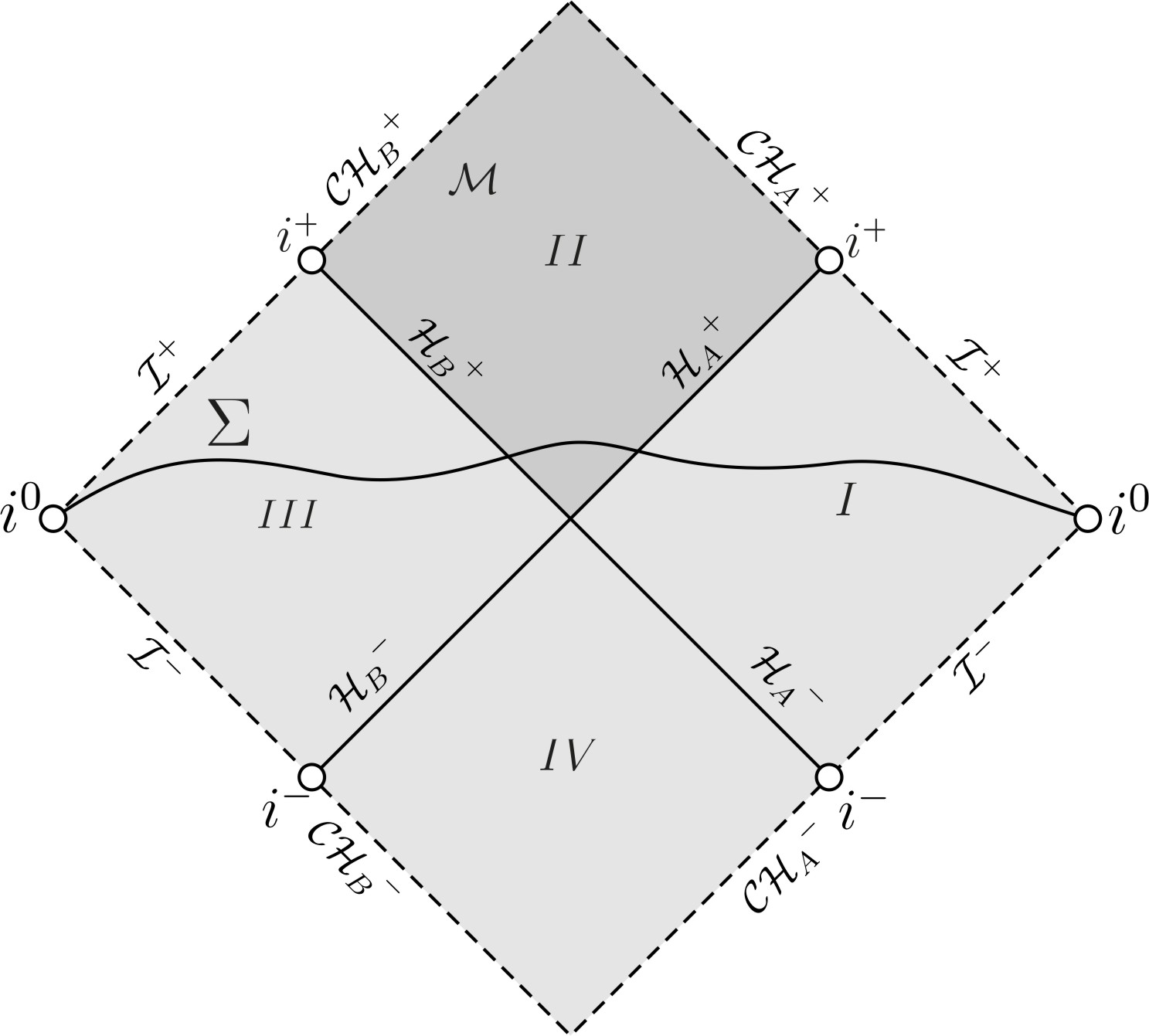
The Kerr spacetime (ℳ,g)({\mathcal{M}},g) is a fundamental axialsymmetric 2-parameter family of solutions to the vacuum Einstein field equations. A brief introduction to the spacetime is given in haw_ellis, and for a more detailed discussion see oneill. The Penrose diagram of the subextremal case, M>|a|≠0M>|a|\neq 0, with aa the angular momentum per unit mass and MM the mass of the black hole, is shown in Figure 1. The problem of analyzing the solution of the scalar wave equation

□g​ψ=0\displaystyle\Box_{g}\psi=0 (1)

on Kerr backgrounds is intimately related to the stability properties of the spacetime itself and to the celebrated Strong Cosmic Censorship Conjecture, see christo_sing and penrose for a presentation of the conjecture.

Refer to caption
Figure 1: Penrose diagram of the maximal future development of a Cauchy hypersurface Σ\Sigma in Kerr spacetime (ℳ,g)({\mathcal{M}},g). What is depicted is in fact the range of a double null coordinate system which is global in the interior and will be discussed further in Section 2.2.3.

The analysis of (1) for the exterior Kerr region J−​(ℐ+)J^{-}({\mathcal{I}}^{+}), in the full subextremal range |a|<M|a|<M, has already been accomplished in m_kerr. The purpose of the present work is to extend the investigation to the interior of the black hole, up to and including the Cauchy horizon 𝒞​ℋ+{\mathcal{C}}{\mathcal{H}}^{+}. The mathematical structure and notation of this paper closely follows our work on Reissner–Nordström backgrounds, see anne.

As already mentioned, the analysis of (1) is motivated by the Strong Cosmic Censorship Conjecture. In order to investigate its validity we need to understand stability and instability properties of black hole interiors. A brief overview on this topic as well as a mathematical formulation of the conjecture were already given in Section 1.2 of anne. References discussing the instability behavior in similar settings are luk_oh; luk_jan. Also refer to simpson for a numerical analysis and poisson; amos; brady for early discussions of heuristic models.

1.1 The main result

The main result of this paper can be stated as follows.

Theorem 1.1.

On subextremal Kerr spacetime (ℳ,g)({\mathcal{M}},g), with mass MM and angular momentum per unit mass aa and M>|a|≠0M>|a|\neq 0, let ψ\psi be a solution of the wave equation □g​ψ=0\Box_{g}\psi=0 arising from sufficiently regular localized Cauchy data on a two-ended asymptotically flat Cauchy surface Σ\Sigma. Then

|ψ|≤C\displaystyle|\psi|\leq C (2)

globally in the black hole interior, in particular up to and including the Cauchy horizon 𝒞​ℋ+{\mathcal{C}}{\mathcal{H}}^{+}, to which ψ\psi extends in fact continuously.

The constant CC is explicitly computable in terms of parameters aa and MM and a suitable norm on initial data. In order to prove the above theorem, we will first derive weighted energy boundedness, as expressed in the following theorem.

Theorem 1.2.

On subextremal Kerr spacetime (ℳ,g)({\mathcal{M}},g), with mass MM and angular momentum per unit mass aa and M>|a|≠0M>|a|\neq 0, let ψ\psi be a solution of the wave equation □g​ψ=0\Box_{g}\psi=0 arising from sufficiently regular localized Cauchy data on a two-ended asymptotically flat Cauchy surface Σ\Sigma. Then, in the black hole interior we have

∫vf​i​x∞∫𝕊u,v2[vp​(∂vψ+bϕ~​∂ϕ~ψ)2​(u,v,θ⋆,ϕ~)+Ω2​|∇⁣/ ​ψ|2​(u,v,θ⋆,ϕ~)]​d​σ𝕊2​𝑑v\displaystyle\int\limits^{\infty}_{v_{fix}}\int\limits_{{\mathbb{S}}^{2}_{u,v}}\left[v^{p}(\partial_{v}\psi+b^{\tilde{\phi}}\partial_{\tilde{\phi}}\psi)^{2}(u,v,\theta^{\star},\tilde{\phi})+\Omega^{2}|\mbox{$\nabla\mkern-13.0mu/$\,}\psi|^{2}(u,v,\theta^{\star},\tilde{\phi})\right]{\mathrm{d}}\sigma_{\mathbb{S}}^{2}{\mathrm{d}}v ≤\displaystyle\leq E,\displaystyle E, (3)
 for vf​i​x≥1v_{fix}\geq 1, u>−∞u>-\infty (4)
∫uf​i​x∞∫𝕊u,v2[up​(∂uψ)2​(u,v,θ⋆,ϕ~)+Ω2​|∇⁣/ ​ψ|2​(u,v,θ⋆,ϕ~)]​d​σ𝕊2​𝑑u\displaystyle\int\limits^{\infty}_{u_{fix}}\int\limits_{{\mathbb{S}}^{2}_{u,v}}\left[u^{p}(\partial_{u}\psi)^{2}(u,v,\theta^{\star},\tilde{\phi})+\Omega^{2}|\mbox{$\nabla\mkern-13.0mu/$\,}\psi|^{2}(u,v,\theta^{\star},\tilde{\phi})\right]{\mathrm{d}}\sigma_{\mathbb{S}}^{2}{\mathrm{d}}u ≤\displaystyle\leq E,\displaystyle E, (5)
for uf​i​x≥1, v>−∞,\displaystyle\quad\mbox{for $u_{fix}\geq 1$, $v>-\infty$}, (6)

where p>1p>1 is an appropriately chosen constant, and (u,v,θ⋆,ϕ~)(u,v,\theta^{\star},\tilde{\phi}) are Eddington–Finkelstein normalized double null coordinates defined in Section 2.2.3. The functions Ω2​(u,v,θ⋆)\Omega^{2}(u,v,\theta^{\star}) and bϕ~​(u,v,θ⋆)b^{\tilde{\phi}}(u,v,\theta^{\star}) are defined by (61) and (62), respectively, together with the metric (58). The expression

d​σ𝕊2=sin⁡θ​d​θ⋆​d​ϕ~\displaystyle{\mathrm{d}}\sigma_{\mathbb{S}}^{2}=\sin\theta{\mathrm{d}}\theta^{\star}{\mathrm{d}}\tilde{\phi} (7)

represents the volume element on the two-spheres 𝕊2{\mathbb{S}}^{2}, which due to the dependence of θ\theta on (u,v,θ⋆)(u,v,\theta^{\star}), stated in (69), do not represent round spheres. Moreover, 𝕊u,v2{\mathbb{S}}^{2}_{u,v} are the two-spheres, which are defined by the intersection of the level sets of uu and vv, we will discuss them more in Section 2.2.3 when we introduce the double null coordinates22 2 We will later introduce a function LL which quantifies the difference between the volume elements of these spheres, see Section 2.2.3 and also (74). Since LL is bounded we are able to omit it in the above statements.. Further, we denote

|∇⁣/ ​ψ|2=(g/ −1)θA​θB​(∂θAψ​∂θBψ).\displaystyle|\mbox{$\nabla\mkern-13.0mu/$\,}\psi|^{2}=(\mbox{$g\mkern-8.0mu/$\,}^{-1})^{\theta_{A}\theta_{B}}(\partial_{\theta_{A}}\psi\partial_{\theta_{B}}\psi). (8)

Remark. Statement (3) for u=−∞u=-\infty and statement (5) for v=−∞v=-\infty hold by previous work on the exterior, see m_kerr; george.

Having obtained Theorem 1.2, commutation by angular momentum operators, using the wave equation itself and estimating error terms of the form (17) leads to a higher order version of the above theorem. The presence of error terms is a difference from the spherically symmetric Reissner–Nordström case, see anne. This will be explained in Section 2.1. The pointwise boundedness of Theorem 1.1 will then follow from the higher order energy theorem and applying Sobolev embedding.

1.2 A first look at the analysis

In the analysis of this paper we are going to use global double null coordinates (u,v,θ⋆,ϕ~)(u,v,\theta^{\star},\tilde{\phi}), which were derived by Pretorius and Israel pretorius and will be discussed in Section 2.2.3. To prove Theorem 1.1 and 1.2 we first consider a characteristic rectangle Ξ\Xi within the black hole interior, whose future right boundary coincides with the Cauchy horizon 𝒞​ℋ+{\mathcal{C}}{\mathcal{H}}^{+} in the vicinity of i+i^{+}, cf.  Figure 2 a), and whose past right boundary coincides with the event horizon ℋ+{\mathcal{H}}^{+}.

Refer to caption
Figure 2: a) Penrose diagram of Kerr spacetime depicting the regions considered in the proof. b) Characteristic rectangle Ξ\Xi, with redshift ℛ{\mathcal{R}}, noshift 𝒩{\mathcal{N}} and blueshift regions ℬ{\mathcal{B}}.

The crux of the entire proof is establishing boundedness of weighted higher order energy norms in Ξ\Xi. Once that is done, analogous results hold for a characteristic rectangle Ξ~\tilde{\Xi} to the left, depicted in Figure 2 a). Hereafter, boundedness of the energy can be propagated to regions ℛV{\mathcal{R}}_{V}, ℛ~V\tilde{{\mathcal{R}}}_{V} and ℛV​I{\mathcal{R}}_{VI} as depicted, proving Theorem 1.2. Commutation by angular momentum operators, controlling the error terms and application of Sobolev embedding then yields Theorem 1.1. For brevity and simplicity we will in fact immediately carry out the commutation and control of error terms in each region. This is to say we directly derive higher order energy estimates for each region respectively.

We will now return to the discussion of Ξ\Xi, since that is the most involved part of the proof. Starting from an upper decay bound for |ψ||\psi| and its derivatives on the event horizon ℋ+{\mathcal{H}}^{+}, we will prove Theorem 1.2 and its higher order version (and hence Theorem 1.1) restricted to Ξ\Xi. This upper bound along ℋ+{\mathcal{H}}^{+} can be deduced from the work of Dafermos et al., cf.  m_kerr and george. We will state the precise required result from previous work in Section 3.1.

In region Ξ\Xi the proof involves distinguishing redshift ℛ={−∞<r⋆≤rr​e​d⋆}{\mathcal{R}}=\left\{-\infty<r^{\star}\leq r^{\star}_{red}\right\}, noshift 𝒩={rr​e​d⋆≤r⋆≤rb​l​u​e⋆}{\mathcal{N}}=\left\{r^{\star}_{red}\leq r^{\star}\leq r^{\star}_{blue}\right\} and blueshift ℬ={rb​l​u​e⋆≤r⋆<∞}{\mathcal{B}}=\left\{r^{\star}_{blue}\leq r^{\star}<\infty\right\} regions, as shown in Figure 2 b).

These regions have appeared in the analysis of the wave equation on Reissner–Nordström backgrounds, cf.  anne and references therein. The analysis is analogous to the previous result, but requires slightly different vector field multipliers and control of error terms. The reader familiar with anne will recognize the structure of the previous proof, which we have maintained here for better readability. A more detailed discussion of the separation into ℛ{\mathcal{R}}, 𝒩{\mathcal{N}} and ℬ{\mathcal{B}} regions is given in Section 2.2.7 and Section 3.2. In region ℬ{\mathcal{B}}, which is adjacent to 𝒞​ℋ+{\mathcal{C}}{\mathcal{H}}^{+}, the weighted vector field

S=|u|p∂u+vp∂v+vpbϕ~∂ϕ~\displaystyle S=|u|^{p}\partial_{u}+v^{p}\partial_{v}+v^{p}b^{\tilde{\phi}}\partial_{\tilde{\phi}}

in Eddington–Finkelstein-like coordinates (u,v)(u,v) is used for the analysis. Note the parameter p>1p>1 appearing in Theorem 1.2. The weights in this vector field, associated to region ℬ{\mathcal{B}}, will allow us to prove uniform boundedness despite the blueshift instability.

1.3 Outline of the paper

The remaining part of the paper is organized as follows.

Section 2 contains all mathematical tools required in order to follow the analysis. In particular, we recall the vector field method in Section 2.1. Moreover, we specify the double-null, Eddington–Finkelstein-like coordinates, in which we will carry out the analysis, in Section 2.2, and introduce more notation in Section 2.3. In Section 3 we give a brief review of the horizon estimates, that follow for the evolution of smooth compactly supported initial data on a Cauchy hypersurface by m_kerr. We also give data on a null hypersurface transverse to the event horizon. Both of these statements together then allow us to propagate the energy estimate further inside, as shown in Section 4.

Section 4 contains the crux of the proof, in which we derive estimates inside a characteristic rectangle Ξ\Xi, as we already explained in Section 1.2. The higher order propagation inside Ξ\Xi is derived in Section 4.1 to 4.4, implying control over all error terms. Hereafter, we derive pointwise estimates inside Ξ\Xi as well as higher order energy estimates in the remaining regions ℛV{\mathcal{R}}_{V}, ℛ~V\tilde{{\mathcal{R}}}_{V} and ℛV​I{\mathcal{R}}_{VI}, see Section 4.5 to 4.7.

In Section 5 we obtain the higher order weighted energy statement for the entire interior and derive pointwise boundedness by using Sobolev embedding on the spheres. We eventually give an outlook in Section 6, in which we put the present work into context and discuss related results.

2 Preliminaries

2.1 Vector field method and energy currents

In the following section we will briefly review the vector field method which we are going to use as an essential tool throughout this work. For an introduction and the history of this method, see sergiu by Klainerman.

The wave equation (1) can be derived from the following matter field Lagrangian

ℒ⁡(ψ)=∫ℳgμ​ν​∂μψ​∂νψ​dVol,{\mathcal{L}}(\psi)=\int_{{\mathcal{M}}}g^{\mu\nu}\partial_{\mu}\psi\partial_{\nu}\psi{\mbox{dVol}}, (9)

on a spacetime manifold (ℳ,g)({\mathcal{M}},g). A symmetric stress-energy tensor can be identified from the variation of the action as

Tμ​ν​(ψ)=∂μψ​∂νψ−12​gμ​ν​gα​β​∂αψ​∂βψ.T_{\mu\nu}(\psi)=\partial_{\mu}\psi\partial_{\nu}\psi-\frac{1}{2}g_{\mu\nu}g^{\alpha\beta}\partial_{\alpha}\psi\partial_{\beta}\psi. (10)

Since ψ\psi is a solution to (1) energy-momentum conservation is implied, i.e.

∇μTμ​ν=0.\nabla^{\mu}T_{\mu\nu}=0. (11)

In this work we will often be interested in the inhomogenous wave equation

□g​ψ~=□g​Y​ψ=F⁡(Y​ψ),\Box_{g}\tilde{\psi}=\Box_{g}Y{\psi}=F(Y{\psi}), (12)

where Y=YθC∂θCY=Y^{\theta_{C}}\partial_{\theta_{C}} is a non-Killing commutation vector field, that will be explained more in Section 2.2.6. The motivation for this is that in order to obtain pointwise estimates we will have to commute with vector fields that are not Killing.

In the remaining section we will define one-currents as well as scalar currents depending on the geometry, which constitute a robust tool for obtaining L2L^{2} estimates. By contracting the energy-momentum tensor with a vector field multiplier VV, we define the current

JμV​(ψ~)≐Tμ​ν​(ψ~)​Vν.J_{\mu}^{V}(\tilde{\psi})\doteq T_{\mu\nu}(\tilde{\psi})V^{\nu}. (13)

If the vector field VV is timelike, then the one-form JμVJ_{\mu}^{V} can be interpreted as an energy flux.

We will frequently apply the divergence theorem, often referred to as Stokes’ theorem, to the above defined energy fluxes (13). Consider for example a spacetime region ℬ\mathcal{B} which is bound by two homologous hypersurfaces, Στ\Sigma_{\tau} and Σ0\Sigma_{0}, then we obtain

∫ΣτJμV​(ψ~)​nΣτμ​dVolΣτ+∫ℬ∇μJμ​(ψ~)​dVol=∫Σ0JμV​(ψ~)​nΣ0μ​dVolΣ0.\int_{\Sigma_{\tau}}J^{V}_{\mu}(\tilde{\psi})n^{\mu}_{\Sigma_{\tau}}{\mbox{dVol}}_{\Sigma_{\tau}}+\int_{\mathcal{B}}\nabla^{\mu}J_{\mu}(\tilde{\psi}){\mbox{dVol}}=\int_{\Sigma_{0}}J^{V}_{\mu}(\tilde{\psi})n^{\mu}_{\Sigma_{0}}{\mbox{dVol}}_{\Sigma_{0}}. (14)

The vector nΣμn^{\mu}_{\Sigma} denotes the normal to the subscript hypersurface Σ\Sigma oriented according to Lorentzian geometry convention. Further, dVol denotes the volume element over the entire spacetime region and dVolΣ{\mbox{dVol}}_{\Sigma} the volume elements on Σ\Sigma, respectively. Using the divergence theorem, we will often estimate the spacetime integral by the boundary terms; or future boundary terms from the sum of past boundary terms and the spacetime integral. In the above example the spacetime integral refers to the second term of the left hand side of (14), the future boundary to the first term and the past boundary to the term on the right hand side of the equation. A proof of the divergence theorem in general can be found in frankel; another useful reference is taylor.

In view of the spacetime integral, we are interested in the divergence of the current (13) which reads as

∇μJμ=∇μ(Tμ​ν​Vν)=Tμ​ν​(∇μVν)+(∇μTμ​ν)​Vν,\nabla^{\mu}J_{\mu}=\nabla^{\mu}(T_{\mu\nu}V^{\nu})=T_{\mu\nu}(\nabla^{\mu}V^{\nu})+(\nabla^{\mu}T_{\mu\nu})V^{\nu}, (15)

and suggests defining the following two scalar currents

KV​(ψ~)≐T⁡(ψ~)​(∇V)=(πV)μ​ν​Tμ​ν​(ψ~),K^{V}(\tilde{\psi})\doteq T(\tilde{\psi})(\nabla V)=(\pi^{V})^{\mu\nu}T_{\mu\nu}(\tilde{\psi}), (16)

where (πV)μ​ν≐12​(ℒV​g)μ​ν(\pi^{V})^{\mu\nu}\doteq\frac{1}{2}({\mathcal{L}}_{V}g)^{\mu\nu} is the so called deformation tensor along VV, and

ℰV​(ψ~)≐(∇μTμ​ν)​Vν=(□g​ψ~)​V​(ψ~).{\mathcal{E}}^{V}(\tilde{\psi})\doteq(\nabla^{\mu}T_{\mu\nu})V^{\nu}=(\Box_{g}\tilde{\psi})V(\tilde{\psi}). (17)

We will sometimes refer to KVK^{V} as “bulk term” and to ℰV{\mathcal{E}}^{V} as “error term”. Thus

∇μJμ=KV+ℰV.\nabla^{\mu}J_{\mu}=K^{V}+{\mathcal{E}}^{V}. (18)

From (16) we see that KVK^{V} is zero in case that our multiplier is a Killing vector field and ℰV{\mathcal{E}}^{V} is zero if ψ~\tilde{\psi} is a solution to the homogeneous wave equation. Recall (12) and suppose for arbitrary ψ~\tilde{\psi} we write ψ~=Y​ψ\tilde{\psi}=Y\psi, with ψ\psi being a solution to (1) and YY an arbitrary vector field, then we see that ℰV{\mathcal{E}}^{V} is zero if [□g,Y]=0[\Box_{g},Y]=0, which is always the case when YY is a Killing vector field. Since in this analysis we are interested in commuting with non-Killing vector fields the error terms will not vanish, but have to be controlled.

2.2 The Kerr solution

In the following we will briefly recall Kerr spacetimes33 3 The reader unfamiliar with this solution may for example consult haw_ellis for a brief review, or the more detailed oneill. which are a family of solutions to the Einstein vacuum field equations

Rμ​ν=0,\displaystyle R_{\mu\nu}=0, (19)

where Rμ​νR_{\mu\nu} is the Ricci tensor. The Kerr solution represents an isolated rotating black hole in an asymptotically flat spacetime and was discovered in 1963, kerr.

For our proofs of Theorem 1.1 and 1.2, it will be favorable to carry out the analysis in double null coordinates. Therefore, in the following sections we will first recall the more widely known Boyer–Lindquist coordinates, to then derive the coordinate transformation leading to the double null form of the metric, first considered by Pretorius and Israel in pretorius.

2.2.1 The metric, ambient differential structure and Killing vector fields

To set the semantic convention, whenever we refer to the Kerr solution (ℳ,g)({\mathcal{M}},g) we mean the maximal domain of dependence 𝒟⁡(Σ)=ℳ{\mathcal{D}}(\Sigma)={\mathcal{M}} of complete two-ended asymptotically flat data Σ\Sigma for the parameter range 0<|a|<M0<|a|<M. The manifold ℳ{\mathcal{M}} can be expressed by ℳ=𝒬×𝕊u,v2{\mathcal{M}}={\mathcal{Q}}\times{\mathbb{S}}^{2}_{u,v}, where 𝕊u,v2{\mathbb{S}}^{2}_{u,v} is defined as the intersection of the level sets of u~\tilde{u} and v~\tilde{v}, for a representation of 𝒬{\mathcal{Q}} see Figure 3. The submanifold ℳ|I​I=𝒬|I​I×𝕊u,v2{\mathcal{M}}|_{II}={\mathcal{Q}}|_{II}\times{\mathbb{S}}^{2}_{u,v}, which is the region of interest, admits global double null coordinates (u,v,θ⋆,ϕ~)(u,v,\theta^{\star},\tilde{\phi}), to be defined in Section 2.2.3, so that we have
Refer to caption
Figure 3: Penrose diagram of maximal domain of dependence of Kerr spacetime with the region of interest shown darker shaded.

𝒬|I​I=[−∞,∞)×[−∞,∞){\mathcal{Q}}|_{II}=[-\infty,\infty)\times[-\infty,\infty) with u,v∈(−∞,∞)u,v\in(-\infty,\infty) and thus

ℳ|I​I=[−∞,∞)×[−∞,∞)×𝕊u,v2.\displaystyle{\mathcal{M}}|_{II}=[-\infty,\infty)\times[-\infty,\infty)\times{\mathbb{S}}^{2}_{u,v}. (20)

We can also formally parametrize the event horizon, the past boundary of 𝒬|I​I{\mathcal{Q}}|_{II}, namely 𝒬|I​I\𝒬̊|I​I{\mathcal{Q}}|_{II}\backslash\mathring{{\mathcal{Q}}}|_{II} by

ℋ+=ℋA+∪ℋB+={−∞}×[−∞,∞)∪[−∞,∞)×{−∞},\displaystyle{\mathcal{H}}^{+}={\mathcal{H}}_{A}^{+}\cup{\mathcal{H}}_{B}^{+}=\left\{-\infty\right\}\times[-\infty,\infty)\cup[-\infty,\infty)\times\left\{-\infty\right\}, (21)

and the future boundary, 𝒬|I​I¯\𝒬|I​I\overline{{\mathcal{Q}}|_{II}}\backslash{\mathcal{Q}}|_{II}, which is a Cauchy horizon by

𝒞ℋ+=𝒞ℋA+∪𝒞ℋB+={∞}×[−∞,∞)∪[−∞,∞)×{∞},\displaystyle{\mathcal{C}}{\mathcal{H}}^{+}={\mathcal{C}}{\mathcal{H}}_{A}^{+}\cup{\mathcal{C}}{\mathcal{H}}_{B}^{+}=\left\{\infty\right\}\times[-\infty,\infty)\cup[-\infty,\infty)\times\left\{\infty\right\}, (22)

where 𝒬̊|I​I\mathring{{\mathcal{Q}}}|_{II} is the interior and 𝒬|I​I¯\overline{{\mathcal{Q}}|_{II}} is the closure of 𝒬|I​I{\mathcal{Q}}|_{II}. The fact that 𝒞​ℋ+{\mathcal{C}}{\mathcal{H}}^{+} is not contained in 𝒬|I​I{\mathcal{Q}}|_{II} is indicated in Figure 4 by the dashed line. The significance of these horizons are discussed further in the following.

Refer to caption
Figure 4: Penrose diagram of region I​III, in which the double null coordinates (u,v,θ⋆,ϕ~)(u,v,\theta^{\star},\tilde{\phi}), to be constructed in Section 2.2.3, are global.

Pretorius and Israel pretorius have already shown the coordinate transformation from the familiar Boyer–Lindquist coordinates to double null coordinates, see also Dafermos et al.  m_rueck. For self containment we will briefly repeat it in Section 2.2.3.

In order to do that, first recall the Kerr metric in Boyer–Lindquist coordinates (t,r,θ,ϕ)(t,r,\theta,\phi):

gB-L=ΣΔ​d​r2+Σ​d​θ2+R2​sin2⁡θ​d​ϕ2−4​M​a​r​sin2⁡θΣ​d​ϕ​d​t−(1−2​M​rΣ)​d​t2,\displaystyle g_{\mbox{\tiny{B-L}}}=\frac{\Sigma}{\Delta}{\mathrm{d}}r^{2}+\Sigma{\mathrm{d}}\theta^{2}+R^{2}\sin^{2}\theta{\mathrm{d}}\phi^{2}-\frac{4Mar\sin^{2}\theta}{\Sigma}{\mathrm{d}}\phi{\mathrm{d}}t-\left(1-\frac{2Mr}{\Sigma}\right){\mathrm{d}}t^{2}, (23)

with

Δ=r2−2​M​r+a2,R2=r2+a2+2​M​a2​r​sin2⁡θΣ,Σ=r2+a2​cos2⁡θ,\displaystyle\Delta=r^{2}-2Mr+a^{2},\quad R^{2}=r^{2}+a^{2}+\frac{2Ma^{2}r\sin^{2}\theta}{\Sigma},\quad\Sigma=r^{2}+a^{2}\cos^{2}\theta, (24)

where MM is the mass and aa is the angular momentum per unit mass of the black hole. Moreover, note the useful identity

Σ​R2=(r2+a2)2−Δ​a2​sin2⁡θ.\displaystyle\Sigma R^{2}=(r^{2}+a^{2})^{2}-\Delta a^{2}\sin^{2}\theta. (25)

Further, θ\theta is the colatitude with

0<θ<π\displaystyle 0<\theta<\pi (26)

and ϕ\phi is the longitude with

0≤ϕ<2​π,\displaystyle 0\leq\phi<2\pi, (27)

so that this coordinate system covers the entire sphere except for the north and south pole. Like in Reissner–Nordström spacetime we have an event horizon ℋ+{\mathcal{H}}^{+} and a Cauchy horizon 𝒞​ℋ+{\mathcal{C}}{\mathcal{H}}^{+} bounding the interior region I​III. The Cauchy horizon is not part of the maximal domain of dependence which is indicated by the dashed line in Figure 3. Both horizons must be stationary null hypersurfaces. Since the normal to any stationary hypersurface is proportional to ∇r\nabla r and lightlike character implies the condition g⁡(∇r,∇r)=gμ​ν​∂μr​∂νr=gr​r=0g(\nabla r,\nabla r)=g^{\mu\nu}\partial_{\mu}r\partial_{\nu}r=g^{rr}=0, we obtain two positive roots

r±=M±M2−a2\displaystyle r_{\pm}=M\pm\sqrt{M^{2}-a^{2}} (28)

of Δ\Delta. Relating this to our yet to be defined (u,v)(u,v) coordinates we can designate the position of the event horizon by

r⁡(−∞,v)=r|ℋA+=r+,r⁡(u,−∞)=r|ℋB+=r+,\displaystyle r(-\infty,v)=r|_{{\mathcal{H}}_{A}^{+}}=r_{+},\qquad r(u,-\infty)=r|_{{\mathcal{H}}_{B}^{+}}=r_{+}, (29)

and the location of the Cauchy horizon by

r(u,∞,)=r|𝒞​ℋA+=r−,r(∞,v)=r|𝒞​ℋB+=r−.\displaystyle r(u,\infty,)=r|_{{\mathcal{C}}{\mathcal{H}}_{A}^{+}}=r_{-},\qquad r(\infty,v)=r|_{{\mathcal{C}}{\mathcal{H}}_{B}^{+}}=r_{-}. (30)

Despite merely having axisymmetry, the surface gravities can be shown to be independent of θ\theta, and thus constant along the horizons44 4 This feature is predicted from the zeroth law of black hole thermodynamics, see toolkit., namely

κ±=r±−Mr±2+a2=±M2−a2r±2+a2,\displaystyle\kappa_{\pm}=\frac{r_{\pm}-M}{r_{\pm}^{2}+a^{2}}=\pm\frac{\sqrt{M^{2}-a^{2}}}{r_{\pm}^{2}+a^{2}}, (31)

where κ+\kappa_{+} is the surface gravity at ℋ±{\mathcal{H}}^{\pm} and κ−\kappa_{-} is the surface gravity at 𝒞​ℋ±{\mathcal{C}}{\mathcal{H}}^{\pm}, see toolkit for further discussion.

Kerr spacetimes exhibit two Killing vector fields ∂t\partial_{t} and ∂ϕ\partial_{\phi}. The linear combination

Tℋ+=∂t+ar+2+a2∂ϕ,\displaystyle T_{{\mathcal{H}}^{+}}=\partial_{t}+\frac{a}{r_{+}^{2}+a^{2}}\partial_{\phi}, (32)

here given in Boyer–Lindquist coordinates, will play a particular role in the analysis inside the redshift region, see Section 4.1. Using (28) we can now also express region 𝒬I​I{\mathcal{Q}}_{II}, the projected region of interest, in terms of a range in rr by

𝒬I​I={r−<r≤r+}.\displaystyle{\mathcal{Q}}_{II}=\left\{r_{-}<r\leq r_{+}\right\}. (33)

We would now like to briefly clarify the causal properties of the Killing vector fields ∂t\partial_{t}, Tℋ+T_{{\mathcal{H}}^{+}} and the vector field ∂r\partial_{r}. In particular, in the interior we have

{∂tspacelike in𝒬̊|I​I,Tℋ+spacelike in𝒬̊|I​I,lightlike atℋ+,∂rtimelike in𝒬̊|I​I,\begin{cases}\partial_{t}&\mbox{spacelike in}\quad\mathring{{\mathcal{Q}}}|_{II},\\ T_{{\mathcal{H}}^{+}}&\mbox{spacelike in}\quad\mathring{{\mathcal{Q}}}|_{II},\quad\mbox{lightlike at}\quad{\mathcal{H}}^{+},\\ \partial_{r}&\mbox{timelike in}\quad\mathring{{\mathcal{Q}}}|_{II},\end{cases} (34)

where 𝒬̊|I​I=𝒬|I​I∖∂𝒬|I​I\mathring{{\mathcal{Q}}}|_{II}={\mathcal{Q}}|_{II}\setminus\partial{\mathcal{Q}}|_{II} is the interior of 𝒬|I​I{\mathcal{Q}}|_{II}. Apart from the two Killing vector fields, there is also a Killing tensor, the so called Carter tensor which will not be used in our analysis.

2.2.2 Defining suitable null coordinates

In our previous paper on Reissner–Nordström interiors, we chose t=v−ut=v-u and r⋆=u+vr^{\star}=u+v, where r⋆r^{\star} was the Regge-Wheeler tortoise coordinate. We will see that the Kerr analog has to have a θ\theta dependence, i. e.  r⋆​(r,θ)r^{\star}(r,\theta). Moreover, we will have to define a coordinate

θ⋆​(r,θ),\displaystyle\theta^{\star}(r,\theta), (35)

where θ⋆\theta^{\star} also has rr and θ\theta dependence and (t,r⋆,θ⋆,ϕ)(t,r^{\star},\theta^{\star},\phi) forms a coordinate system in (ℳ,g)({\mathcal{M}},g). All the sign differences compared to m_rueck and pretorius appearing in this section, arise from choices, which are appropriate for the analysis in the interior region as opposed to the exterior region of the black hole and are in agreement with the interior analysis of m_luk.

As explained in pretorius and in more detail in Appendix A of m_luk, we first define θ⋆∈[θ,π2)\theta^{\star}\in[\theta,\frac{\pi}{2}) implicitly in the following: For r∈[r−,r+],θ∈(0,π2)r\in[r_{-},r_{+}],\theta\in(0,\frac{\pi}{2}),

F⁡(r,θ,θ⋆)=∫θ⋆θd​θ′P⁡(θ′,θ⋆)+∫rr+d​r′Q⁡(r′,θ⋆)=0,\displaystyle F(r,\theta,\theta^{\star})=\int\limits_{\theta^{\star}}^{\theta}\frac{{\mathrm{d}}\theta^{\prime}}{P(\theta^{\prime},\theta^{\star})}+\int\limits_{r}^{r_{+}}\frac{{\mathrm{d}}r^{\prime}}{Q(r^{\prime},\theta^{\star})}=0, (36)

with

P2​(θ,θ⋆)=a2​(sin2⁡θ⋆−sin2⁡θ)andQ2​(r,θ⋆)=(r2+a2)2−a2​sin2⁡θ⋆​Δ,\displaystyle P^{2}(\theta,\theta^{\star})=a^{2}(\sin^{2}\theta^{\star}-\sin^{2}\theta)\qquad\mbox{and}\qquad Q^{2}(r,\theta^{\star})=(r^{2}+a^{2})^{2}-a^{2}\sin^{2}\theta^{\star}\Delta, (37)

and

P≥0,Q>0.\displaystyle P\geq 0,\qquad Q>0. (38)

For the range θ∈(π2,π)\theta\in(\frac{\pi}{2},\pi), the coordinate θ⋆\theta^{\star} is defined by

θ⋆​(r,θ)=π−θ⋆​(r,π−θ).\displaystyle\theta^{\star}(r,\theta)=\pi-\theta^{\star}(r,\pi-\theta). (39)

And further, we fix

θ⋆​(r,0)=0,θ⋆​(r,π2)=π2,θ⋆​(r,π)=π,\displaystyle\theta^{\star}(r,0)=0,\qquad\theta^{\star}(r,\frac{\pi}{2})=\frac{\pi}{2},\qquad\theta^{\star}(r,{\pi})={\pi}, (40)

for r∈[r−,r+]r\in[r_{-},r_{+}]. It was shown in Appendix A of m_luk that equations (36), (39) and (40) define a unique θ⋆\theta^{\star}. Further, we define ρ\rho by

ρ⁡(r,θ,θ⋆)\displaystyle\rho(r,\theta,\theta^{\star}) =\displaystyle= ∫θ⋆θP⁡(θ′,θ⋆)​d​θ′+∫r+rQ⁡(r′,θ⋆)Δ​d​r′+ρ⁡(r+−ϵ,0,0)\displaystyle\int\limits_{\theta^{\star}}^{\theta}{P(\theta^{\prime},\theta^{\star})}{{\mathrm{d}}\theta^{\prime}}+\int\limits_{r_{+}}^{r}\frac{Q(r^{\prime},\theta^{\star})}{\Delta}{{\mathrm{d}}r^{\prime}}+\rho({r_{+}-\epsilon},0,0) (41)
=\displaystyle= ∫θ⋆θP⁡(θ′,θ⋆)​d​θ′−∫rr+Q⁡(r′,θ⋆)Δ​d​r′+ρ⁡(r+,0,0)\displaystyle\int\limits_{\theta^{\star}}^{\theta}{P(\theta^{\prime},\theta^{\star})}{{\mathrm{d}}\theta^{\prime}}-\int\limits_{r}^{r_{+}}\frac{Q(r^{\prime},\theta^{\star})}{\Delta}{{\mathrm{d}}r^{\prime}}+\rho({r_{+}},0,0)
=\displaystyle= ∫θ⋆θP⁡(θ′,θ⋆)​d​θ′+∫rr+r′2+a2−Q⁡(r′,θ⋆)Δ​d​r′+[∫r+rr′2+a2Δ​d​r′+ρ⁡(r+,0,0)]\displaystyle\int\limits_{\theta^{\star}}^{\theta}{P(\theta^{\prime},\theta^{\star})}{{\mathrm{d}}\theta^{\prime}}+\int\limits_{r}^{r_{+}}\frac{{r^{\prime}}^{2}+a^{2}-Q(r^{\prime},\theta^{\star})}{\Delta}{{\mathrm{d}}r^{\prime}}+\left[\int\limits_{r_{+}}^{r}\frac{{r^{\prime}}^{2}+a^{2}}{\Delta}{{\mathrm{d}}r^{\prime}}+\rho({r_{+}},0,0)\right]
=\displaystyle= ∫θ⋆θP⁡(θ′,θ⋆)​d​θ′+∫rr+r′2+a2−Q⁡(r′,θ⋆)Δ​d​r′+∫crr′2+a2Δ​d​r′.\displaystyle\int\limits_{\theta^{\star}}^{\theta}{P(\theta^{\prime},\theta^{\star})}{{\mathrm{d}}\theta^{\prime}}+\int\limits_{r}^{r_{+}}\frac{{r^{\prime}}^{2}+a^{2}-Q(r^{\prime},\theta^{\star})}{\Delta}{{\mathrm{d}}r^{\prime}}+\int\limits_{c}^{r}\frac{{r^{\prime}}^{2}+a^{2}}{\Delta}{{\mathrm{d}}r^{\prime}}.

The arrangement in the radial dependence was made to ensure convergence of the definite integral despite Δ\Delta approaching zero at the horizons. Because of (35) we can now define

r⋆​(r,θ)=ρ⁡(θ⋆​(r,θ),r,θ),\displaystyle r^{\star}(r,\theta)=\rho(\theta^{\star}(r,\theta);r,\theta), (42)

where r⋆∈(−∞,∞)r^{\star}\in(-\infty,\infty) as r ranges between r+r_{+} and r−r_{-} and for the partial derivatives we obtain

∂r⋆∂r=QΔ,∂r⋆∂θ=P.\displaystyle\frac{\partial r^{\star}}{\partial r}=\frac{Q}{\Delta},\qquad\frac{\partial r^{\star}}{\partial\theta}=P. (43)

It is easy to see from the eikonal equation, that ∂r⋆\partial_{r^{\star}} is a future directed timelike vector field in the interior and r⋆=c​o​n​s​tr^{\star}=const is a spacelike hypersurface. As already pointed out in pretorius, with this construction of r⋆r^{\star} the variables

v=t+r⋆​(r,θ)2,u=r⋆​(r,θ)−t2\displaystyle v=\frac{t+{r}^{\star}(r,\theta)}{2},\qquad u=\frac{r^{\star}(r,\theta)-t}{2} (44)

are lightlike and satisfy

gα​β​(∂αv)​(∂βv)=14​Σ​[Δ​(∂rr⋆)2+(∂θr⋆)2−(r2+a2)2Δ+a2​sin2⁡θ]=0,\displaystyle g^{\alpha\beta}(\partial_{\alpha}v)(\partial_{\beta}v)=\frac{1}{4\Sigma}\left[\Delta(\partial_{r}{r}^{\star})^{2}+(\partial_{\theta}{r}^{\star})^{2}-\frac{(r^{2}+a^{2})^{2}}{\Delta}+a^{2}\sin^{2}\theta\right]=0, (45)

together with the analog for the uu coordinate.

Now we are ready to summarize all differentials, which we are going to use in Section 2.2.3 to derive the Kerr metric in double null coordinates. From a straight forward calculation we get

d​r\displaystyle{\mathrm{d}}r =\displaystyle= Q​ΔΣ​R2​(d​v+d​u)+G​Q​P2​ΔΣ​R2​d​θ⋆,\displaystyle\frac{Q\Delta}{\Sigma R^{2}}({\mathrm{d}}v+{\mathrm{d}}u)+\frac{GQP^{2}\Delta}{\Sigma R^{2}}{\mathrm{d}}\theta^{\star}, (46)
d​θ\displaystyle{\mathrm{d}}\theta =\displaystyle= P​ΔΣ​R2​(d​v+d​u)−G​P​Q2Σ​R2​d​θ⋆,\displaystyle\frac{P\Delta}{\Sigma R^{2}}({\mathrm{d}}v+{\mathrm{d}}u)-\frac{GPQ^{2}}{\Sigma R^{2}}{\mathrm{d}}\theta^{\star}, (47)

with

G⁡(r⋆,θ⋆)≡∂θ⋆F,\displaystyle G(r^{\star},\theta^{\star})\equiv\partial_{\theta^{\star}}F, (48)

where rr and θ\theta are fixed for the partial derivative ∂θ⋆\partial_{\theta^{\star}}. The exact expression was given in Proposition A.2 of Appendix A of m_luk.

2.2.3 Eddington–Finkelstein normalized double null coordinates

In the following we will carry out the coordinate transformation (r,t,ϕ,θ)→(u,v,ϕ~,θ⋆)(r,t,\phi,\theta)\rightarrow(u,v,\tilde{\phi},\theta^{\star}), since double null coordinates will turn out more convenient for our interior analysis. Using (46), (47) and d​t=d​v−d​u{\mathrm{d}}t={\mathrm{d}}v-{\mathrm{d}}u in (23) we obtain

gKerr=4​ΔR2​d​u​d​v+L2R2​d​θ⋆2+R2​sin2⁡θ​(d​ϕ−ωB​(d​v−d​u))2,\displaystyle g_{\mbox{\tiny{Kerr}}}=4\frac{\Delta}{R^{2}}{\mathrm{d}}u{\mathrm{d}}v+\frac{L^{2}}{R^{2}}{\mathrm{d}}{\theta^{\star}}^{2}+R^{2}\sin^{2}\theta({\mathrm{d}}\phi-\omega_{B}({\mathrm{d}}v-{\mathrm{d}}u))^{2}, (49)

where we have defined

L⁡(u,v,θ⋆)≡−G​P​Q,\displaystyle L(u,v,\theta^{\star})\equiv-GPQ, (50)
ωB​(u,v,θ⋆)=2​M​a​rΣ​R2.\displaystyle\omega_{B}(u,v,\theta^{\star})=\frac{2Mar}{\Sigma R^{2}}. (51)

Note that the quantities QQ and −G​P-GP, given in (37) and (48) are positive and bounded from above and below in the interior region. In particular,

P\displaystyle P ≲\displaystyle\lesssim |a|​sin⁡(2​θ⋆),\displaystyle|a|{\sin(2\theta^{\star})}, (52)

since sin2⁡θ⋆−sin2⁡θ≲sin⁡(2​θ⋆)\sqrt{\sin^{2}\theta^{\star}-\sin^{2}\theta}\lesssim\sin(2\theta^{\star}), as shown in Appendix A of m_luk. Also notice that

Σ​R2=P2​Δ+Q2=(r2+a2)2−a2​Δ​sin2⁡θ,\displaystyle\Sigma R^{2}=P^{2}\Delta+Q^{2}=(r^{2}+a^{2})^{2}-a^{2}\Delta\sin^{2}\theta, (53)

so the quantity is bounded in the interior region. Further, refer to Proposition A.3 of m_luk where the following proposition was proven.

Proposition 2.1.

(M.  Dafermos and J.  Luk) Suppose F⁡(θ⋆,r,θ)=0F(\theta^{\star};r,\theta)=0. Then

−cM,a≤P⁡(θ⋆,θ)​∂∂θ⋆|r,θ​fixed​F​(θ⋆,r,θ)≤−sin⁡(2​θ)sin⁡(2​θ⋆)<−CM,a,\displaystyle-{c_{M,a}}\leq\left.P(\theta^{\star};\theta)\frac{\partial}{\partial\theta^{\star}}\right|_{r,\theta\mbox{\tiny{fixed}}}F(\theta^{\star};r,\theta)\leq-\frac{\sin(2\theta)}{\sin(2\theta^{\star})}<-C_{M,a}, (54)

for some constants cM,a,CM,a>0c_{M,a},C_{M,a}>0 depending on MM and aa.

The proposition together with (50) and the boundedness above and below of QQ then lead to the boundedness

0<c<L⁡(u,v,θ⋆)≤C.\displaystyle 0<c<L(u,v,\theta^{\star})\leq C. (55)

Let us now use the coordinate transformation55 5 The constant multiplying vv in transformation (56) is added in hindsight. It will render the parameter bϕ~b^{\tilde{\phi}}, see (62), zero at 𝒞​ℋ+{\mathcal{C}}{\mathcal{H}}^{+}.

ϕ\displaystyle\phi =\displaystyle= ϕ~+h⁡(u,v,θ⋆)+4​M​a​rΣ​R2|r=r−⋅v,\displaystyle\tilde{\phi}+h(u,v,\theta^{\star})+\left.\frac{4Mar}{\Sigma R^{2}}\right|_{r=r_{-}}\cdot v, (56)
d​ϕ\displaystyle{\mathrm{d}}\phi =\displaystyle= d​ϕ~+∂θ⋆h​d​θ⋆+∂uh​d​u+(∂vh+4​M​a​rΣ​R2|r=r−)​d​v,\displaystyle{\mathrm{d}}\tilde{\phi}+\partial_{\theta^{\star}}h{\mathrm{d}}\theta^{\star}+\partial_{u}h{\mathrm{d}}u+\left(\partial_{v}h+\left.\frac{4Mar}{\Sigma R^{2}}\right|_{r=r_{-}}\right){\mathrm{d}}v, (57)

with h⁡(u,v,θ⋆)h(u,v,\theta^{\star}) a function for which we require that ∂uh=∂vh=−ωB\partial_{u}h=\partial_{v}h=-\omega_{B} and with initial data h⁡(r⋆=0,θ⋆)=0h(r^{\star}=0;\theta^{\star})=0. This leads to the following more convenient form of the metric in Eddington–Finkelstein normalized double null coordinates which were already related to the well known Boyer–Lindquist coordinates in pretorius and m_rueck:

g=−2​Ω2​(u,v,θ⋆)​(d​u⊗d​v+d​v⊗d​u)+g/ θC​θD​(d​θC−bθC​d​v)⊗(d​θD−bθD​d​v),\displaystyle g=-2\Omega^{2}(u,v,\theta^{\star})({\mathrm{d}}u\otimes{\mathrm{d}}v+{\mathrm{d}}v\otimes{\mathrm{d}}u)+\mbox{$g\mkern-8.0mu/$\,}_{\theta_{C}\theta_{D}}({\mathrm{d}}\theta_{C}-b^{\theta_{C}}{\mathrm{d}}v)\otimes({\mathrm{d}}\theta_{D}-b^{\theta_{D}}{\mathrm{d}}v), (58)

with C,D=1,2C,D=1,2 and θ1\theta_{1}, θ2\theta_{2} denoting θ⋆\theta^{\star} and ϕ~{\tilde{\phi}} respectively. Further,

g/ θC​θD​(u,v,θ⋆,ϕ~)\displaystyle\mbox{$g\mkern-8.0mu/$\,}_{\theta_{C}\theta_{D}}(u,v,\theta^{\star},{\tilde{\phi}})\quad is a Riemannian metric on 𝕊u,v2,\displaystyle\mbox{is a Riemannian metric on ${\mathbb{S}}^{2}_{u,v}$}, (59)
bθC​(u,v,θ⋆,ϕ~)\displaystyle b^{\theta_{C}}(u,v,\theta^{\star},{\tilde{\phi}})\quad is a vector field taking values in the tangent space of 𝕊u,v2.\displaystyle\mbox{is a vector field taking values in the tangent space of ${\mathbb{S}}^{2}_{u,v}$}.

For the inverse metric we then obtain

g−1\displaystyle g^{-1} =\displaystyle= −12​Ω2​(u,v,θ⋆)(∂u⊗∂v+∂v⊗∂u)−12​Ω2​(u,v,θ⋆)bθC(∂u⊗∂θC+∂θC⊗∂u)\displaystyle-\frac{1}{2\Omega^{2}(u,v,\theta^{\star})}(\partial_{u}\otimes\partial_{v}+\partial_{v}\otimes\partial_{u})-\frac{1}{2\Omega^{2}(u,v,\theta^{\star})}b^{\theta_{C}}(\partial_{u}\otimes\partial_{\theta_{C}}+\partial_{\theta_{C}}\otimes\partial_{u}) (60)
+(g/ −1)θC​θD(∂θC⊗∂θD).\displaystyle+(\mbox{$g\mkern-8.0mu/$\,}^{-1})^{\theta_{C}\theta_{D}}(\partial_{\theta_{C}}\otimes\partial_{\theta_{D}}).

Further, for the metric coefficients we obtain

Ω2=−ΔR2,\displaystyle\Omega^{2}=-\frac{\Delta}{R^{2}}, (61)
bθ⋆=0,bϕ~=2​ωB​(u,v,θ⋆)−4​M​a​rΣ​R2|r=r−=(51)4​M​a​rΣ​R2−4​M​a​rΣ​R2|r=r−,\displaystyle b^{\theta^{\star}}=0,\quad b^{\tilde{\phi}}=2\omega_{B}(u,v,\theta^{\star})-\left.\frac{4Mar}{\Sigma R^{2}}\right|_{r=r_{-}}\stackrel{{\scriptstyle\eqref{omega_B}}}{{=}}\frac{4Mar}{\Sigma R^{2}}-\left.\frac{4Mar}{\Sigma R^{2}}\right|_{r=r_{-}}, (62)
g/ ϕ~​ϕ~=R2​sin2⁡θ,\displaystyle\mbox{$g\mkern-8.0mu/$\,}_{\tilde{\phi}\tilde{\phi}}=R^{2}\sin^{2}\theta, (63)
g/ θ⋆​θ⋆=L2R2+(∂h∂θ⋆)2​R2​sin2⁡θ,\displaystyle\mbox{$g\mkern-8.0mu/$\,}_{\theta^{\star}\theta^{\star}}=\frac{L^{2}}{R^{2}}+\left(\frac{\partial h}{\partial\theta^{\star}}\right)^{2}R^{2}\sin^{2}\theta, (64)
g/ θ⋆​ϕ~=(∂h∂θ⋆)​R2​sin2⁡θ,\displaystyle\mbox{$g\mkern-8.0mu/$\,}_{\theta^{\star}\tilde{\phi}}=\left(\frac{\partial h}{\partial\theta^{\star}}\right)R^{2}\sin^{2}\theta, (65)
(g/ ϕ~​ϕ~)−1=1R2​sin2⁡θ+(∂h∂θ⋆)2​R2L2,\displaystyle(\mbox{$g\mkern-8.0mu/$\,}^{\tilde{\phi}\tilde{\phi}})^{-1}=\frac{1}{R^{2}\sin^{2}\theta}+\left(\frac{\partial h}{\partial\theta^{\star}}\right)^{2}\frac{R^{2}}{L^{2}}, (66)
(g/ θ⋆​θ⋆)−1=R2L2,\displaystyle(\mbox{$g\mkern-8.0mu/$\,}^{\theta^{\star}\theta^{\star}})^{-1}=\frac{R^{2}}{L^{2}}, (67)
(g/ θ⋆​ϕ~)−1=−(∂h∂θ⋆)​R2L2.\displaystyle(\mbox{$g\mkern-8.0mu/$\,}^{\theta^{\star}\tilde{\phi}})^{-1}=-\left(\frac{\partial h}{\partial\theta^{\star}}\right)\frac{R^{2}}{L^{2}}. (68)

Recall again that the coordinate ϕ~\tilde{\phi} was chosen such that bϕ~b^{\tilde{\phi}} vanishes at 𝒞​ℋ+{\mathcal{C}}{\mathcal{H}}^{+}. Moreover, by (46), from which we can read off ∂θ⋆r\partial_{\theta^{\star}}r, together with (61), we can see that ∂θ⋆bϕ~\partial_{\theta^{\star}}b^{\tilde{\phi}} is proportional to Ω2\Omega^{2} and thus also vanishes at 𝒞​ℋ+{\mathcal{C}}{\mathcal{H}}^{+}, compare with Section 2.2.5. This is shown in more detail in Appendix A of m_luk, where also smoothness at the poles for the angular variables (θ⋆,ϕ~)(\theta^{\star},\tilde{\phi}) is shown.

Further, note that we have the following dependencies

r=r⁡(u,v,θ⋆),θ=θ⁡(u,v,θ⋆),\displaystyle r=r(u,v,\theta^{\star}),\qquad\theta=\theta(u,v,\theta^{\star}), (69)
L=L(u,v,θ⋆),h=h(u,v,θ⋆),R=R(u,v,θ⋆), cf.  (24).\displaystyle L=L(u,v,\theta^{\star}),\qquad h=h(u,v,\theta^{\star}),\qquad R=R(u,v,\theta^{\star}),\mbox{ cf.~ \eqref{sigma_usw}}. (70)

These dependencies are crucial since together with (81) and (82) we will see that derivatives of these quantities with respect to uu and vv will also decay like Ω2\Omega^{2}. We will explain this more in Section 2.2.5.

2.2.4 The volume elements

From the expression for the metric we derive the volume elements for the entire spacetime

dVol =\displaystyle= 2​Ω2​L​sin⁡θ​d​θ⋆​d​ϕ~​d​u​d​v,\displaystyle 2\Omega^{2}L\sin\theta{\mathrm{d}}\theta^{\star}{\mathrm{d}}\tilde{\phi}{\mathrm{d}}u{\mathrm{d}}v, (71)

as well as for the 3-dimensional hypersurfaces along constant r⋆r^{\star} values:

dVolr⋆=c​o​n​s​t\displaystyle{\mbox{dVol}}_{{r^{\star}=const}} =\displaystyle= 2​Ω2​L​sin⁡θ​d​θ⋆​d​ϕ~​d​r⋆,\displaystyle\sqrt{2\Omega^{2}}L\sin\theta{\mathrm{d}}\theta^{\star}{\mathrm{d}}\tilde{\phi}{\mathrm{d}}r^{\star}, (72)

were we have used

−g=2​Ω2​gθ⋆​θ⋆​gϕ~​ϕ~−gθ⋆​ϕ~2=2​Ω2​L​sin⁡θ.\displaystyle\sqrt{-g}=2\Omega^{2}\sqrt{g_{\theta^{\star}\theta^{\star}}g_{\tilde{\phi}\tilde{\phi}}-g_{\theta^{\star}\tilde{\phi}}^{2}}=2\Omega^{2}L\sin\theta. (73)

Note that the induced volume element of our spheres 𝕊u,v2{\mathbb{S}^{2}_{u,v}}, which are not round spheres, but are defined as the intersections of the level sets of uu and vv, is given by

d​σ𝕊u,v2\displaystyle{\mathrm{d}}\sigma_{\mathbb{S}^{2}_{u,v}} =\displaystyle= −g/ ​d​θ⋆​d​ϕ~=L​sin⁡θ​d​θ⋆​d​ϕ~=L​d​σ𝕊2,\displaystyle\sqrt{-\mbox{$g\mkern-8.0mu/$\,}}{\mathrm{d}}\theta^{\star}{\mathrm{d}}\tilde{\phi}=L\sin\theta{\mathrm{d}}\theta^{\star}{\mathrm{d}}\tilde{\phi}=L{\mathrm{d}}\sigma_{\mathbb{S}^{2}}, (74)

see (7). Therefore, we see that L⁡(u,v,θ⋆)L(u,v,\theta^{\star}) plays the role of a radial coordinate which also varies in θ⋆\theta^{\star}. Moreover, the normal vectors on constant u,vu,v hypersurfaces and their related volume elements appearing in the statements of our theorems are given by:

nv=c​o​n​s​tμ\displaystyle n^{\mu}_{{v=const}} =∂u,\displaystyle=\partial_{u},\qquad\qquad\qquad dVolv=c​o​n​s​t=2​Ω2​L​sin⁡θ​d​θ⋆​d​ϕ~​d​u,\displaystyle{\mbox{dVol}}_{{v=const}}=2\Omega^{2}L\sin\theta{\mathrm{d}}\theta^{\star}{\mathrm{d}}\tilde{\phi}{\mathrm{d}}u, (75)
nu=c​o​n​s​tμ\displaystyle n^{\mu}_{{u=const}} =∂v+bϕ~∂ϕ~,\displaystyle=\partial_{v}+b^{\tilde{\phi}}\partial_{\tilde{\phi}},\qquad dVolu=c​o​n​s​t=2​Ω2​L​sin⁡θ​d​θ⋆​d​ϕ~​d​v.\displaystyle{\mbox{dVol}}_{{u=const}}=2\Omega^{2}L\sin\theta{\mathrm{d}}\theta^{\star}{\mathrm{d}}\tilde{\phi}{\mathrm{d}}v. (76)

2.2.5 Boundedness of all required coefficients

In order to carry out the analysis in the interior we will require the following relations of the parameters introduced in the previous sections.

∂r∂r⋆\displaystyle\frac{\partial r}{\partial r^{\star}} =\displaystyle= Δ​QΣ​R2,∂r∂θ⋆=Δ​PΣ​R2\displaystyle\frac{\Delta Q}{\Sigma R^{2}},\qquad\frac{\partial r}{\partial{\theta^{\star}}}=\frac{\Delta P}{\Sigma R^{2}} (77)
∂θ∂r⋆\displaystyle\frac{\partial\theta}{\partial r^{\star}} =\displaystyle= Δ​PΣ​R2,∂θ∂θ⋆=−G​P​Q2Σ​R2.\displaystyle\frac{\Delta P}{\Sigma R^{2}},\qquad\frac{\partial\theta}{\partial{\theta^{\star}}}=-\frac{GPQ^{2}}{\Sigma R^{2}}. (78)

These relations are valid since ∂θ⋆∂r\frac{\partial\theta^{\star}}{\partial r} and ∂θ⋆∂θ\frac{\partial\theta^{\star}}{\partial\theta} are finite, which was proven in Appendix A.3 of m_luk. Further, recall (52) and the statement above of it together with (53) which imply

|∂r∂r⋆|≲|Δ|,|∂r∂θ⋆|≲|Δ|​sin⁡(2​θ⋆),\displaystyle\left|\frac{\partial r}{\partial r^{\star}}\right|\lesssim\left|\Delta\right|,\qquad\left|\frac{\partial r}{\partial{\theta^{\star}}}\right|\lesssim\left|\Delta\right|\sin(2\theta^{\star}), (79)
|∂θ∂r⋆|≲|Δ|​sin⁡(2​θ⋆),|∂θ∂θ⋆|≲1,\displaystyle\left|\frac{\partial\theta}{\partial r^{\star}}\right|\lesssim\left|\Delta\right|\sin(2\theta^{\star}),\qquad\left|\frac{\partial\theta}{\partial{\theta^{\star}}}\right|\lesssim 1, (80)

as also stated in m_luk. Note that the sign of QQ was chosen to be positive so the sign of ∂r∂r⋆\frac{\partial r}{\partial r^{\star}} is negative. Moreover, for the partial derivatives of (r,θ)(r,\theta) with respect to (u,v)(u,v) we have

∂ζr=∂r⋆∂ζ​∂r∂r⋆=(77)Δ​QΣ​R2,\displaystyle\partial_{\zeta}r=\frac{\partial r^{\star}}{\partial\zeta}\frac{\partial r}{\partial r^{\star}}\stackrel{{\scriptstyle\eqref{r_rstar}}}{{=}}\frac{\Delta Q}{\Sigma R^{2}}, (81)
∂ζθ=∂r⋆∂ζ​∂θ∂r⋆=(78)Δ​PΣ​R2,\displaystyle\partial_{\zeta}\theta=\frac{\partial r^{\star}}{\partial\zeta}\frac{\partial\theta}{\partial r^{\star}}\stackrel{{\scriptstyle\eqref{theta_rstar}}}{{=}}\frac{\Delta P}{\Sigma R^{2}}, (82)

with ∂ζr\partial_{\zeta}r and ∂ζθ\partial_{\zeta}\theta negative, and ζ=u,v\zeta=u,v. Note that the entire analysis will be discussed in r⋆r^{\star} coordinates not in rr coordinates, where in the region r−<r<r+r_{-}<r<r_{+} all r⋆=c​o​n​s​tr^{\star}=const hypersurfaces are spacelike hypersurfaces and r⋆∈(−∞,∞)r^{\star}\in(-\infty,\infty).

Further, to close the proof of our main theorem we will need to show boundedness of our metric coefficients and their derivatives up to second order. For this we repeat Proposition A.6 and Remark A.11 of Appendix A of m_luk.

Proposition 2.2.

(M. Dafermos and J. Luk) For every fixed k≤2k\leq 2, rr and θ\theta are CkC^{k} functions of r⋆r^{\star} and θ⋆\theta^{\star}. Moreover, the following bounds hold with implicit constants depending on kk (in addition to MM and aa):

∑1≤k1≤k−1|(1sin⁡(2​θ⋆)​∂∂θ⋆)k1​(∂θ∂θ⋆)|≲1,\displaystyle\sum\limits_{1\leq k_{1}\leq k-1}\left|\left(\frac{1}{\sin(2\theta^{\star})}\frac{\partial}{\partial\theta^{\star}}\right)^{k_{1}}\left(\frac{\partial\theta}{\partial\theta^{\star}}\right)\right|\lesssim 1, (83)
∑1≤k1≤k|(∂θ∂r⋆)k1​θ|≲|Δ|​sin⁡(2​θ⋆),\displaystyle\sum\limits_{1\leq k_{1}\leq k}\left|\left(\frac{\partial\theta}{\partial r^{\star}}\right)^{k_{1}}\theta\right|\lesssim|\Delta|\sin(2\theta^{\star}), (84)
∑1≤k1+k2≤k−1;k2≥1|(1sin⁡(2​θ⋆)​∂∂θ⋆)k1​(∂∂r⋆)k2​(∂∂θ⋆)|≲|Δ|,\displaystyle\sum\limits_{1\leq k_{1}+k_{2}\leq k-1;k_{2}\geq 1}\left|\left(\frac{1}{\sin(2\theta^{\star})}\frac{\partial}{\partial\theta^{\star}}\right)^{k_{1}}\left(\frac{\partial}{\partial r^{\star}}\right)^{k_{2}}\left(\frac{\partial}{\partial\theta^{\star}}\right)\right|\lesssim|\Delta|, (85)
∑1≤k1+k2≤k|(∂∂r⋆)k1​(1sin⁡(2​θ⋆)​∂∂θ⋆)k2​r|≲|Δ|.\displaystyle\sum\limits_{1\leq k_{1}+k_{2}\leq k}\left|\left(\frac{\partial}{\partial r^{\star}}\right)^{k_{1}}\left(\frac{1}{\sin(2\theta^{\star})}\frac{\partial}{\partial\theta^{\star}}\right)^{k_{2}}r\right|\lesssim|\Delta|. (86)

Recall the functions bϕ~(u,v,θ⋆)=2ωB−4​M​a​rΣ​R2|r=r−b^{\tilde{\phi}}(u,v,\theta{\star})=2\omega_{B}-\left.\frac{4Mar}{\Sigma R^{2}}\right|_{r=r_{-}} of (62) and dh(u,v,θ⋆)d​r⋆=−ωB\frac{{\mathrm{d}}h(u,v,\theta{\star})}{{\mathrm{d}}r^{\star}}=-\omega_{B} appering in (56), with (51). With the help of (79) we can now state

|∂bϕ~(u,v,θ⋆)∂r⋆|≲|Δ|.\displaystyle\left|\frac{\partial b^{\tilde{\phi}}(u,v,\theta{\star})}{\partial r^{\star}}\right|\lesssim|\Delta|. (87)

We further make use of the following.

Remark 2.3.

(M. Dafermos and J. Luk) Notice that using

∂∂θ⋆​(4​M​a​rΣ​R2)=∂r∂θ⋆​∂∂r​(4​M​a​rΣ​R2)+∂θ∂θ⋆​∂∂θ​(4​M​a​rΣ​R2)\displaystyle\frac{\partial}{\partial\theta^{\star}}\left(\frac{4Mar}{\Sigma R^{2}}\right)=\frac{\partial r}{\partial\theta^{\star}}\frac{\partial}{\partial r}\left(\frac{4Mar}{\Sigma R^{2}}\right)+\frac{\partial\theta}{\partial\theta^{\star}}\frac{\partial}{\partial\theta}\left(\frac{4Mar}{\Sigma R^{2}}\right) (88)

together with

|∂∂θ​(4​M​a​rΣ​R2)|=|4​M​a3​r​sin⁡(2​θ)​Δ((r2+a2)2−a2​sin2⁡θ​Δ)2|≲|Δ|​|sin⁡(2​θ⋆)|\displaystyle\left|\frac{\partial}{\partial\theta}\left(\frac{4Mar}{\Sigma R^{2}}\right)\right|=\left|\frac{4Ma^{3}r\sin(2\theta)\Delta}{((r^{2}+a^{2})^{2}-a^{2}\sin^{2}\theta\Delta)^{2}}\right|\lesssim|\Delta||\sin(2\theta^{\star})| (89)

and estimates (79)-(80), we have

|∂∂θ⋆​(4​M​a​rΣ​R2)|≲|Δ|​|sin⁡(2​θ⋆)|.\displaystyle\left|\frac{\partial}{\partial\theta^{\star}}\left(\frac{4Mar}{\Sigma R^{2}}\right)\right|\lesssim|\Delta||\sin(2\theta^{\star})|. (90)

As a consequence, the expression ∂h∂θ⋆\frac{\partial h}{\partial\theta^{\star}} that appears in the metric component, compare (62), (63) and (65), satisfies the following bound

|∂h∂θ⋆|≲|sin⁡(2​θ⋆)|.\displaystyle\left|\frac{\partial h}{\partial\theta^{\star}}\right|\lesssim|\sin(2\theta^{\star})|. (91)

We moreover make use of Proposition A.12 of Appendix A of m_luk, which we are not repeating here. Further, we obtain

|2​∂δL​sin⁡θL​sin⁡θ|=|∂δ(L2​sin2⁡θ)L2​sin2⁡θ|=|2​∂δLL+2​cos⁡θsin⁡θ​∂δθ|≲|Δ|,\displaystyle\left|2\frac{\partial_{\delta}L\sin\theta}{L\sin\theta}\right|=\left|\frac{\partial_{\delta}(L^{2}\sin^{2}\theta)}{L^{2}\sin^{2}\theta}\right|=\left|2\frac{\partial_{\delta}L}{L}+2\frac{\cos\theta}{\sin\theta}\partial_{\delta}\theta\right|\lesssim|\Delta|, (92)

with δ=u,v\delta=u,v and where we used (79), (80) and Proposition A.2 of m_luk. This will turn out useful since we have to control this term in Section 4.4. Moreover, we have

(g/ −1)θC​θD​∂ηg/ θC​θD=∂ηdetg/ detg/ =∂η(L2​sin2⁡θ)L2​sin2⁡θ,\displaystyle(\mbox{$g\mkern-8.0mu/$\,}^{-1})^{\theta_{C}\theta_{D}}\partial_{\eta}\mbox{$g\mkern-8.0mu/$\,}_{\theta_{C}\theta_{D}}=\frac{\partial_{\eta}\mbox{det}\mbox{$g\mkern-8.0mu/$\,}}{\mbox{det}\mbox{$g\mkern-8.0mu/$\,}}=\frac{\partial_{\eta}(L^{2}\sin^{2}\theta)}{L^{2}\sin^{2}\theta}, (93)

is a term appearing in our bulk term, with η=u,v,θ⋆,ϕ~\eta=u,v,\theta^{\star},\tilde{\phi}, see (238) and also in the wave equation, see (263). Note here, that ∂θ⋆|L​sin⁡θ||L​sin⁡θ|\frac{\partial_{\theta^{\star}}|L\sin\theta|}{|L\sin\theta|} is not bounded, but the product of this term and the volume element is.

2.2.6 Angular momentum operators

In this section we define the angular momentum operators by the vector fields

Yi=YθCi∂θC=Yiθ⋆∂θ⋆+Yiϕ~∂ϕ~,\displaystyle Y_{i}=Y^{\theta_{C}}_{i}\partial_{\theta_{C}}=Y_{i}^{\theta^{\star}}\partial_{\theta^{\star}}+Y_{i}^{\tilde{\phi}}\partial_{\tilde{\phi}}, (94)

where YiθC=YiθC​(θ⋆,ϕ~)Y_{i}^{\theta_{C}}=Y_{i}^{\theta_{C}}(\theta^{\star},\tilde{\phi}), C=1,2C=1,2 and θ1=θ⋆\theta_{1}=\theta^{\star}, θ2=ϕ~\theta_{2}=\tilde{\phi} and i=1,2,3i=1,2,3. Further, we fix Y3θ⋆=0Y_{3}^{\theta^{\star}}=0 and Y3ϕ~=1Y_{3}^{\tilde{\phi}}=1, so that

Y3=∂ϕ~,\displaystyle Y_{3}=\partial_{\tilde{\phi}}, (95)

which is Killing for Kerr spacetimes. The YiY_{i} vector fields represent the standard generators (with respect to the (θ⋆,ϕ~)(\theta^{\star},{\tilde{\phi}}) coordinates) of the Lie algebra s​o​(3)so(3) acting on the spheres 𝕊u,v2{\mathbb{S}}^{2}_{u,v}. Since only Y3Y_{3} is Killing in Kerr spacetime, only the abelian subalgebra u(1)=⟨∂ϕ~⟩⊂so(3)u(1)=\left\langle\partial_{\tilde{\phi}}\right\rangle\subset so(3) acts by isometries. As we can see from (58), the two null vectors are orthogonal to YiY_{i}, namely ⟨∂u,∂θC⟩=0\langle\partial_{u},\partial_{\theta_{C}}\rangle=0 and ⟨∂v+bθD∂θD,∂θC⟩=0\langle\partial_{v}+b^{\theta_{D}}\partial_{\theta_{D}},\partial_{\theta_{C}}\rangle=0, with D=1,2D=1,2. More generally we will use YkY^{k}, with the upper index k∈{0,1,2}k\in\left\{0,1,2\right\} to refer to the summation of the required number of commutations, expressed by

JμX​(Yk​ψ)​nμ\displaystyle J_{\mu}^{X}(Y^{k}\psi)n^{\mu} ≐\displaystyle\doteq ∑i1=13⋯∑ik=13JμX(Yi1⋯(Yikψ))nμ,\displaystyle\sum\limits_{i_{1}=1}^{3}\cdot\cdot\cdot\sum\limits_{i_{k}=1}^{3}J_{\mu}^{X}(Y_{i_{1}}\cdot\cdot\cdot(Y_{i_{k}}\psi))n^{\mu}, (96)

where ij=1,2,3i_{j}=1,2,3. To make it more explicit, we can write

JμX​(Y0​ψ)​nμ\displaystyle J_{\mu}^{X}(Y^{0}\psi)n^{\mu} ≐\displaystyle\doteq JμX​(ψ)​nμ,\displaystyle J_{\mu}^{X}(\psi)n^{\mu}, (97)
JμX​(Y1​ψ)​nμ\displaystyle J_{\mu}^{X}(Y^{1}\psi)n^{\mu} ≐\displaystyle\doteq ∑i1=13JμX​(Yi1​ψ)​nμ=JμX​(Y1​ψ)​nμ+JμX​(Y2​ψ)​nμ+JμX​(Y3​ψ)​nμ,\displaystyle\sum\limits_{i_{1}=1}^{3}J_{\mu}^{X}(Y_{i_{1}}\psi)n^{\mu}=J_{\mu}^{X}(Y_{1}\psi)n^{\mu}+J_{\mu}^{X}(Y_{2}\psi)n^{\mu}+J_{\mu}^{X}(Y_{3}\psi)n^{\mu}, (98)
JμX​(Y2​ψ)​nμ\displaystyle J_{\mu}^{X}(Y^{2}\psi)n^{\mu} ≐\displaystyle\doteq ∑i1=13∑i2=13JμX​(Yi1​(Yi2​ψ))​nμ\displaystyle\sum\limits_{i_{1}=1}^{3}\sum\limits_{i_{2}=1}^{3}J_{\mu}^{X}(Y_{i_{1}}(Y_{i_{2}}\psi))n^{\mu} (99)
=\displaystyle= JμX​(Y1​(Y1​ψ))​nμ+JμX​(Y1​(Y2​ψ))​nμ+JμX​(Y1​(Y3​ψ))​nμ\displaystyle\quad J_{\mu}^{X}(Y_{1}(Y_{1}\psi))n^{\mu}+J_{\mu}^{X}(Y_{1}(Y_{2}\psi))n^{\mu}+J_{\mu}^{X}(Y_{1}(Y_{3}\psi))n^{\mu}
+JμX​(Y2​(Y1​ψ))​nμ+JμX​(Y2​(Y2​ψ))​nμ+JμX​(Y2​(Y3​ψ))​nμ\displaystyle+J_{\mu}^{X}(Y_{2}(Y_{1}\psi))n^{\mu}+J_{\mu}^{X}(Y_{2}(Y_{2}\psi))n^{\mu}+J_{\mu}^{X}(Y_{2}(Y_{3}\psi))n^{\mu}
+JμX​(Y3​(Y1​ψ))​nμ+JμX​(Y3​(Y2​ψ))​nμ+JμX​(Y3​(Y3​ψ))​nμ.\displaystyle+J_{\mu}^{X}(Y_{3}(Y_{1}\psi))n^{\mu}+J_{\mu}^{X}(Y_{3}(Y_{2}\psi))n^{\mu}+J_{\mu}^{X}(Y_{3}(Y_{3}\psi))n^{\mu}.

Similar to (96), one can define summed expressions for KX​(Yk​ψ)K^{X}(Y^{k}\psi) and ℰX​(Yk​ψ){\mathcal{E}}^{X}(Y^{k}\psi). In our proof we will also estimate absolute values of these quantities, which we express by

|KX​(Yk​ψ)|\displaystyle\left|K^{X}(Y^{k}\psi)\right| ≐\displaystyle\doteq ∑i1=13⋯∑ik=13|KX(Yi1⋯(Yikψ))|,\displaystyle\sum\limits_{i_{1}=1}^{3}\cdot\cdot\cdot\sum\limits_{i_{k}=1}^{3}\left|K^{X}(Y_{i_{1}}\cdot\cdot\cdot(Y_{i_{k}}\psi))\right|, (100)

and

|ℰX​(Yk​ψ)|\displaystyle\left|{\mathcal{E}}^{X}(Y^{k}\psi)\right| ≐\displaystyle\doteq ∑i1=13⋯∑ik=13|ℰX(Yi1⋯(Yikψ))|.\displaystyle\sum\limits_{i_{1}=1}^{3}\cdot\cdot\cdot\sum\limits_{i_{k}=1}^{3}\left|{\mathcal{E}}^{X}(Y_{i_{1}}\cdot\cdot\cdot(Y_{i_{k}}\psi))\right|. (101)

2.2.7 The redshift, noshift and blueshift region

As we have already mentioned in the introduction, in the interior we can distinguish

redshift ℛ={−∞<r⋆≤r⋆r​e​d},\displaystyle\mbox{${\mathcal{R}}=\left\{-\infty<r^{\star}\leq r^{\star}_{red}\right\}$}, (102)
noshift 𝒩={r⋆r​e​d≤r⋆≤r⋆b​l​u​e},\displaystyle\mbox{${\mathcal{N}}=\left\{r^{\star}_{red}\leq r^{\star}\leq r^{\star}_{blue}\right\}$}, (103)
and blueshift ℬ={rb​l​u​e⋆≤r⋆<∞}{\mathcal{B}}=\left\{r^{\star}_{blue}\leq r^{\star}<\infty\right\} (104)

subregions, as shown in Figure 5.

Refer to caption
Figure 5: Penrose diagram of the interior with distinction into redshift ℛ{\mathcal{R}}, noshift 𝒩{\mathcal{N}} and blueshift ℬ{\mathcal{B}} regions.

In the redshift region ℛ{\mathcal{R}}, we make use of the fact that the surface gravity κ+\kappa_{+} of the event horizon is positive, see (31). Let φt\varphi_{t} and φϕ\varphi_{{\phi}} denote the 1-parameter groups of diffeomorphisms generated by the Killing fields ∂t\partial_{t} and ∂ϕ\partial_{\phi} (in Boyer-Lindquist coordinates), respectively. Then, the redshift region is characterized by the fact that there exists a φt\varphi_{t} and φϕ\varphi_{{\phi}} invariant vector field NN, such that its associated current JμN​nv=c​o​n​s​tμJ^{N}_{\mu}n^{\mu}_{v=const} on a v=c​o​n​s​tv=const hypersurface can be controlled by the related bulk term KNK^{N}, cf.  Proposition 4.1. This property of the bulk term KNK^{N} holds sufficiently close to ℋ+{\mathcal{H}}^{+}. In particular, we shall define rr​e​d⋆r^{\star}_{red} negative and with big enough absolute value such that Proposition 4.1 is applicable. (Furthermore, note that the quantity ∂ζΩΩ\frac{\partial_{\zeta}\Omega}{\Omega} is always positive in ℛ{\mathcal{R}}.)

In 𝒩{\mathcal{N}}, defined in (103), we exploit the fact that JUJ^{U}, KUK^{U} and ℰU{\mathcal{E}}^{U} are invariant under translations along ∂t\partial_{t}, where tt is the Boyer–Lindquist coordinate. For that reason we can uniformly control the bulk by the current along a constant r⋆r^{\star} hypersurface. This will be explained further in Section 4.2.

The blueshift region ℬ{\mathcal{B}} is characterized by the fact that the bulk term KS0K^{S_{0}}, associated to the vector field S0S_{0}, to be defined in (136), is positive. We define rb​l​u​e⋆r^{\star}_{blue} big enough such that the quantities

∂ζΩΩ=12​[∂ζΔΔ−∂ζ(R2)R2],\displaystyle\frac{\partial_{\zeta}\Omega}{\Omega}=\frac{1}{2}\left[\frac{\partial_{\zeta}\Delta}{\Delta}-\frac{\partial_{\zeta}(R^{2})}{R^{2}}\right], (105)

with ζ=u,v\zeta=u,v, carry a negative sign66 6 Readers familiar with anne might notice that, for |a|≪M|a|\ll M, the quantity in (105) defining the sign approaches M−a2rM-\frac{a^{2}}{r} which is analogous to the charged case with aa in place of the charge ee.. In particular, for ϵ~\tilde{\epsilon} sufficiently small the following lower bound holds in ℬ{\mathcal{B}}

0<β≤−2​∂uΩΩ,0<β≤−2​∂vΩΩ,\displaystyle 0<{\beta}\leq-2\frac{\partial_{u}\Omega}{\Omega},\qquad 0<{\beta}\leq-2\frac{\partial_{v}\Omega}{\Omega}, (106)

with β\beta a positive constant.

2.3 Notation

It will be useful to determine in- and outgoing null hypersurfaces from intersection of out- and ingoing null hypersurfaces with the spacelike hypersurfaces r⋆=rr​e​d⋆r^{\star}=r^{\star}_{red}, r⋆=rb​l​u​e⋆r^{\star}=r^{\star}_{blue} and in addition the hypersurface γ\gamma which will be defined in Section 4.3.1. In order to do that, recall the beginning of Section 2.2.1 and end of Section 2.2.3, were we have expressed the submanifold ℳ|I​I=𝒬|I​I×𝕊u,v2{\mathcal{M}}|_{II}={\mathcal{Q}}|_{II}\times{\mathbb{S}}^{2}_{u,v} by (20). Further, we define ℳ|I​I=π−1​(𝒬|I​ICLOSE{\mathcal{M}}|_{II}=\pi^{-1}({\mathcal{Q}}|_{II}), where π\pi is the projection π:ℳ|I​I→𝒬|I​I\pi:{\mathcal{M}}|_{II}\rightarrow{\mathcal{Q}}|_{II}. Now we are able to define functions that are evaluated by the projection π\pi of two particular intersecting hypersurfaces. For example given the hypersurface r⋆=rr​e​d⋆r^{\star}=r^{\star}_{red} and the hypersurface u=u~u=\tilde{u} we define the vv value at which these two hypersurfaces intersect by a function vr​e​d​(u~)v_{red}(\tilde{u}) evaluated for u~\tilde{u}. Let us therefore introduce the following notation:

vr​e​d​(u~)\displaystyle v_{red}(\tilde{u})\qquad is determined by r⋆​(vr​e​d​(u~),u~)=rr​e​d⋆,\displaystyle\qquad r^{\star}(v_{red}(\tilde{u}),\tilde{u})=r^{\star}_{red},
vγ​(u~)\displaystyle v_{\gamma}(\tilde{u})\qquad is determined by (vγ​(u~),u~)∈γ,\displaystyle\qquad(v_{\gamma}(\tilde{u}),\tilde{u})\in\gamma,
vb​l​u​e​(u~)\displaystyle v_{blue}(\tilde{u})\qquad is determined by r⋆​(vb​l​u​e​(u~),u~)=rb​l​u​e,\displaystyle\qquad r^{\star}(v_{blue}(\tilde{u}),\tilde{u})=r_{blue},
ur​e​d​(v~)\displaystyle u_{red}(\tilde{v})\qquad is determined by r⋆​(ur​e​d​(v~),v~)=rr​e​d⋆,\displaystyle\qquad r^{\star}(u_{red}(\tilde{v}),\tilde{v})=r^{\star}_{red},
uγ​(v~)\displaystyle u_{\gamma}(\tilde{v})\qquad is determined by (uγ​(v~),v~)∈γ,\displaystyle\qquad(u_{\gamma}(\tilde{v}),\tilde{v})\in\gamma,
ub​l​u​e​(v~)\displaystyle u_{blue}(\tilde{v})\qquad is determined by r⋆​(ub​l​u​e​(v~),v~)=rb​l​u​e⋆.\displaystyle\qquad r^{\star}(u_{blue}(\tilde{v}),\tilde{v})=r^{\star}_{blue}. (107)

For a better understanding the reader may refer to Figure 6.

Refer to caption
Figure 6: Sketch of blueshift region ℬ{\mathcal{B}}, with quantities depicted a) dependent on u~\tilde{u} and b) dependent on v~\tilde{v}.

Note that the above functions are well defined since r⋆=rr​e​d⋆r^{\star}=r^{\star}_{red}, r⋆=rb​l​u​e⋆r^{\star}=r^{\star}_{blue} and γ\gamma are spacelike hypersurfaces along which we have uγ​(v)→−∞u_{\gamma}(v)\rightarrow-\infty as v→∞v\rightarrow\infty.

3 The setup

3.1 Horizon estimates and Cauchy stability

Our starting point will be decay bounds for ψ\psi, proven by Dafermos, Rodnianski and Shlapentokh-Rothman m_kerr. In particular they show decay for ψ\psi and its derivatives in the black hole exterior up to and including the event horizon for the full range of all subextremal Kerr solutions. More specifically, the following theorem was stated in estimate (21)(21) of Theorem 3.1 and (26)(26) of Theorem 3.2 of m_kerr, where the coordinate τ\tau is comparable to our coordinate vv. Also see the improved decay rate in george derived by Moschidis.

Theorem 3.1.

Let ψ\psi be a solution of the wave equation (1) on a subextremal Kerr background (ℳ,g)({\mathcal{M}},g), with mass MM and angular momentum per unit mass aa and M>|a|≠0M>|a|\neq 0, arising from smooth compactly supported initial data on an arbitrary Cauchy hypersurface Σ\Sigma, cf.  Figure 1. Then, there exists δ>0\delta>0 such that

∫vv+1∫𝕊u,v2[(∂vYk​ψ+bϕ~​∂ϕ~Yk​ψ)2​(−∞,v)+Ω2​|∇⁣/ ​Yk​ψ|2​(−∞,v)]​L​d​σ𝕊2​𝑑v≤C​v−2−2​δ,\displaystyle\int\limits^{v+1}_{v}\int\limits_{{\mathbb{S}}^{2}_{u,v}}\left[(\partial_{v}Y^{k}\psi+b^{\tilde{\phi}}\partial_{\tilde{\phi}}Y^{k}\psi)^{2}(-\infty,v)+\Omega^{2}|\mbox{$\nabla\mkern-13.0mu/$\,}Y^{k}\psi|^{2}(-\infty,v)\right]L{\mathrm{d}}\sigma_{\mathbb{S}^{2}}{\mathrm{d}}v\leq Cv^{-2-2\delta}, (108)

on ℋA+{{\mathcal{H}}_{A}}^{+}, for all vv, with YkY^{k} as in (94), all k∈{0,1,2}k\in\left\{0,1,2\right\} and some positive constants CC depending on the initial data.

The expression 𝕊u,v2{{\mathbb{S}}^{2}_{u,v}} denotes the spheres obtained in Eddington-Finkelstein-like coordinates which were derived in Section 2.2.3. The assumption of smoothness and compact support in Theorem 3.1 can be weakened. See also related results anderson; tataru; tataru2; luk2; m_I_kerr; m_lec; m_bound for the |a|≪M|a|\ll M case and bernard; yakov for mode stability.

Moreover, trivially from Cauchy stability, boundedness of the energy along a null segment transverse to ℋ+{\mathcal{H}}^{+} can be derived. See Section 1.2 and recall that we have chosen the v=1v=1 hypersurface to be the past boundary of the characteristic rectangle Ξ\Xi. More generally we can state the following proposition.

Proposition 3.2.

Let u⋄,v⋄∈(−∞,∞)u_{\diamond},v_{\diamond}\in(-\infty,\infty). Under the assumption of Theorem 3.1, the energy at advanced Eddington–Finkelstein-like coordinate {v=v⋄}∩{−∞≤u≤u⋄}\left\{v=v_{\diamond}\right\}\cap\left\{{-\infty}\leq u\leq{u_{\diamond}}\right\} is bounded from the initial data

∫−∞u⋄∫𝕊u,v2[(∂uYk​ψ)2​(u,v⋄)+Ω2​|∇⁣/ ​Yk​ψ|2​(u,v⋄)]​L​d​σ𝕊2​𝑑u\displaystyle\int\limits_{-\infty}^{u_{\diamond}}\int\limits_{{\mathbb{S}}^{2}_{u,v}}\left[(\partial_{u}Y^{k}\psi)^{2}(u,v_{\diamond})+{\Omega^{2}}|\mbox{$\nabla\mkern-13.0mu/$\,}Y^{k}\psi|^{2}(u,v_{\diamond})\right]L{\mathrm{d}}\sigma_{\mathbb{S}^{2}}{\mathrm{d}}u ≤\displaystyle\leq D⁡(u⋄,v⋄),\displaystyle D(u_{\diamond},v_{\diamond}), (109)

with YkY^{k} as in (94) and for all k∈{0,1,2}k\in\left\{0,1,2\right\}. Further,

sup−∞≤u≤u⋄∫𝕊u,v2(Yk​ψ)2​(u,v⋄)​d​σ𝕊2\displaystyle\sup_{-\infty\leq u\leq{u_{\diamond}}}\int\limits_{{\mathbb{S}}^{2}_{u,v}}(Y^{k}\psi)^{2}(u,v_{\diamond}){\mathrm{d}}\sigma_{\mathbb{S}^{2}} ≤\displaystyle\leq D⁡(u⋄,v⋄),\displaystyle D(u_{\diamond},v_{\diamond}), (110)

with D⁡(u⋄,v⋄)D(u_{\diamond},v_{\diamond}) positive constants depending on the initial data on Σ\Sigma.

Proof. This follows immediately from local energy estimates in a compact spacetime region. Note the Ω2\Omega^{2} weights which arise since uu is not regular at ℋA+{\mathcal{H}}^{+}_{A}.   ∎

3.2 Statement of the theorem and outline of the proof in the neighborhood of i+i^{+}

Before we can prove Theorem 1.1, we will first show the following.

Theorem 3.3.

On subextremal Kerr spacetime with M>|a|≠0M>|a|\neq 0, let ψ\psi be as in Theorem 3.1, then

|ψ|≤C\displaystyle|\psi|\leq C

in the black hole interior up to 𝒞​ℋ+{\mathcal{C}}{\mathcal{H}}^{+} in a “small neighbourhood” of timelike infinity i+i^{+}, that is in (−∞,u✂]×[1,∞)(-\infty,u_{\text{✂}}]\times[1,\infty) for some u✂>−∞u_{\text{✂}}>-\infty.

Remark. We will see that CC depends only on the initial data.

First we consider the right side of the spacetime interior. In particular we consider a characteristic rectangle Ξ\Xi which extends from ℋA+{\mathcal{H}}_{A}^{+}, as shown in Figure 7.

Refer to caption
Figure 7: a) Depiction of characteristic rectangle Ξ\Xi within 𝒬|I​I{\mathcal{Q}}|_{II} of Kerr spacetime, b) region Ξ\Xi zoomed in.

We pick the characteristic rectangle to be defined by Ξ={(−∞≤u≤u✂),(1≤v<∞)}\Xi=\left\{(-\infty\leq u\leq u_{\text{✂}}),(1\leq v<\infty)\right\}, where u✂u_{\text{✂}} is sufficiently close to −∞-\infty for reasons that will become clear later on, cf.  Lemma 4.14 and Proposition 4.15. Bounds on the data along the event horizon ℋA+{\mathcal{H}}_{A}^{+} were stated in Theorem 3.1, and bounds on the data of the transverse null segment were given in Proposition 3.2. Both are consequences of propagation of smooth initial data from a Cauchy hypersurface as explained in Section 3. Theorem 3.3 will be proven by first deriving energy estimates in the distinguished regions, denoted by redshift ℛ{\mathcal{R}}, the noshift 𝒩{\mathcal{N}} and the blueshift ℬ{\mathcal{B}} region, with the properties as explained in Section 2.2.7, cf.  Figure 7 b). According to the properties of these regions we will have to choose different vector field mutlipliers in each of them.

In the redshift region ℛ{\mathcal{R}} we will make use of the redshift vector field NN, already introduced in m_lec. We will elaborate more on this in Section 4.1. Proposition 4.1 proves the positivity of the bulk KNK^{N} which leads to boundedness of the energy flux generated by the current JμN​nv=c​o​n​s​tμJ^{N}_{\mu}n^{\mu}_{v=const}. Here we will have to construct NN, as explained in Section 4.1, such that it can also compensate for the appearing error terms after commuting twice with the angular momentum operators. Applying the divergence theorem, decay up to r⋆=rr​e​d⋆r^{\star}=r^{\star}_{red} will be proven.

In the noshift region 𝒩{\mathcal{N}}, we can simply appeal to the fact that the future directed timelike vector field

U=∂u+∂v+bϕ~∂ϕ~,\displaystyle U=\partial_{u}+\partial_{v}+b^{\tilde{\phi}}\partial_{\tilde{\phi}},

is invariant under the flow of the spacelike Killing vector field ∂t\partial_{t}. It is for that reason that the bulk terms KUK^{U} as well as the error terms ℰU{\mathcal{E}}^{U} can be uniformly controlled by the energy flux JμU​nr⋆=r¯⋆μJ_{\mu}^{U}n^{\mu}_{{r^{\star}}=\bar{r}^{\star}} through the r⋆=r¯⋆{r^{\star}}=\bar{r}^{\star} hypersurface. Decay up to r⋆=rb​l​u​e⋆r^{\star}=r^{\star}_{blue} will be proven by making use of this, together with the uniform boundedness of the vv length of the region that we cut in 𝒩{\mathcal{N}}.

In order to gain control in the blueshift region ℬ{\mathcal{B}}, we will partition it by the hypersurface γ\gamma admitting logarithmic distance in vv from r⋆=rb​l​u​e⋆r^{\star}=r^{\star}_{blue}, cf.  Section 4.3.1. We will then separately consider the region to the past of γ\gamma, J−​(γ)∩ℬJ^{-}(\gamma)\cap{\mathcal{B}}, and the region to the future of γ\gamma, J+​(γ)∩ℬJ^{+}(\gamma)\cap{\mathcal{B}}. The region to the future of γ\gamma is characterized by good decay bounds on Ω2\Omega^{2}. This property will be crucial to derive estimates for bulk and error terms in the future of γ\gamma.

In J−​(γ)∩ℬJ^{-}(\gamma)\cap{\mathcal{B}} we use a vector field

S0=fq∂r⋆=fq(∂u+∂v+bϕ~∂ϕ~),\displaystyle{S_{0}}=f^{q}\partial_{r^{\star}}=f^{q}(\partial_{u}+\partial_{v}+b^{\tilde{\phi}}\partial_{\tilde{\phi}}),

where qq is sufficiently large, and ff is a function with certain properties defined in Section 4.3.2. Choosing the parameter qq big enough renders the terms associated to the spacetime integral positive, which is the “good” sign, when using the divergence theorem to derive upper bounds.

In order to complete the proof, we consider finally the region J+​(γ)∩ℬJ^{+}(\gamma)\cap{\mathcal{B}} and propagate the decay further from the hypersurface γ\gamma, up to the Cauchy horizon in a neighborhood of i+i^{+}. For this, we introduce a new timelike vector field S{S} defined by

S=|u|p∂u+vp∂v+vpbϕ~∂ϕ~,\displaystyle{S}=|u|^{p}\partial_{u}+v^{p}\partial_{v}+v^{p}b^{\tilde{\phi}}\partial_{\tilde{\phi}}, (111)

for an arbitrary pp such that

1<p≤1+2​δ,\displaystyle 1<p\leq 1+2\delta, (112)

where δ\delta is as in Theorem 3.1. We use pointwise estimates on Ω2\Omega^{2} in J+​(γ)J^{+}(\gamma) as a crucial step, see Section 4.4.1. This is due to the proportionality of the occurring quantities to the function Ω2\Omega^{2}, see Section 2.2.5.

Putting everything together, in view of the geometry and the weights of SS, we finally obtain for all v∗≥1v_{*}\geq 1

∫1v∗∫𝕊u,v2vp​(∂vYk​ψ)2​L​sin⁡θ​d​θ⋆​𝑑ϕ~​𝑑v≲Data,\displaystyle\int\limits_{1}^{v_{*}}\int\limits_{{\mathbb{S}}^{2}_{u,v}}v^{p}(\partial_{v}Y^{k}\psi)^{2}L\sin\theta{\mathrm{d}}\theta^{\star}{\mathrm{d}}\tilde{\phi}{\mathrm{d}}v\lesssim\mbox{Data}, (113)

for the weighted flux, with YkY^{k} as in Section 2.2.6. Using the above, the uniform boundedness for ψ\psi stated in Theorem 3.3 can then be derived from an argument that can be sketched as follows.

Let us first see how we obtain an integrated bound on the spheres. By the fundamental theorem of calculus and the Cauchy–Schwarz inequality we get

∫𝕊u,v2(Yk​ψ)2​(u,v∗,θ⋆,ϕ~)​L​sin⁡θ​d​θ⋆​𝑑ϕ~\displaystyle\int\limits_{{\mathbb{S}}^{2}_{u,v}}(Y^{k}\psi)^{2}(u,v_{*},\theta^{\star},\tilde{\phi})L\sin\theta{\mathrm{d}}\theta^{\star}{\mathrm{d}}\tilde{\phi} (114)
≲\displaystyle\lesssim ∫𝕊u,v2(∫1v∗vp​(∂vYk​ψ)2​𝑑v)​(∫1v∗v−p​𝑑v)​L​sin⁡θ​d​θ⋆​𝑑ϕ~+data\displaystyle\int\limits_{{\mathbb{S}}^{2}_{u,v}}\left(\int\limits_{1}^{v_{*}}v^{p}(\partial_{v}Y^{k}\psi)^{2}{\mathrm{d}}v\right)\left(\int\limits_{1}^{v_{*}}v^{-p}{\mathrm{d}}v\right)L\sin\theta{\mathrm{d}}\theta^{\star}{\mathrm{d}}\tilde{\phi}+\mbox{data}
≲\displaystyle\lesssim (∫1v∗∫𝕊u,v2vp​(∂vYk​ψ)2​L​sin⁡θ​d​θ⋆​𝑑ϕ~​𝑑v)​(∫1v∗v−p​𝑑v)+data,\displaystyle\left(\int\limits_{1}^{v_{*}}\int\limits_{{\mathbb{S}}^{2}_{u,v}}v^{p}(\partial_{v}Y^{k}\psi)^{2}L\sin\theta{\mathrm{d}}\theta^{\star}{\mathrm{d}}\tilde{\phi}{\mathrm{d}}v\right)\left(\int\limits_{1}^{v_{*}}v^{-p}{\mathrm{d}}v\right)+\mbox{data},

where the bound (55) allowed us to pull the (L​sin⁡θ)(L\sin\theta)-factor of the volume form inside the integral, so that the first factor of the first term is controlled by (113). Therefore, we further get

∫𝕊u,v2(Yk​ψ)2​L​sin⁡θ​d​θ⋆​𝑑ϕ~≲(113)Data​∫1v∗v−p​𝑑v+data≲Data+data,\displaystyle\int\limits_{{\mathbb{S}}^{2}_{u,v}}(Y^{k}\psi)^{2}L\sin\theta{\mathrm{d}}\theta^{\star}{\mathrm{d}}\tilde{\phi}\stackrel{{\scriptstyle\eqref{fluxscetch}}}{{\lesssim}}\mbox{Data}\int\limits_{1}^{v_{*}}v^{-p}{\mathrm{d}}v+\mbox{data}\lesssim\mbox{Data}+\mbox{data}, (115)

where we have used ∫1∞v−p​𝑑v<∞\int\limits^{\infty}_{1}v^{-p}{\mathrm{d}}v<\infty which followed from the first inequality of (112).

Obtaining a pointwise statement from the above will be achieved by using (115) and applying Sobolev embedding on the spheres 𝕊u,v2{\mathbb{S}}^{2}_{u,v} (which are not round spheres), thus leads to the desired bounds, see Section 4.5.2. This will close the proof of Theorem 3.3. Having only one spacelike symmetry and having to control the appearing error terms is one of the main difficulties of this paper in comparison to the Reissner–Nordström analog anne.

4 Energy estimates in the interior

4.1 Propagation through the redshift region ℛ{\mathcal{R}} to r⋆=rr​e​d⋆r^{\star}=r^{\star}_{red}

The following proposition was shown in m_lec, see also volker for a detailed proof.

Proposition 4.1.

(M. Dafermos and I. Rodnianski) For rr​e​d⋆r^{\star}_{red} sufficiently close to −∞-\infty there exists a φt\varphi_{t} and φϕ\varphi_{\phi}-invariant smooth future directed timelike vector field NN on {−∞<r⋆≤rr​e​d⋆}∩{v≥1}\left\{-\infty<r^{\star}\leq r^{\star}_{red}\right\}\cap\left\{v\geq 1\right\} and a positive constant b0b_{0} such that

b0​JμN​(ψ)​nvμ≤KN​(ψ),\displaystyle b_{0}J_{\mu}^{N}(\psi)n^{\mu}_{{v}}\leq K^{N}(\psi), (116)

for all solutions ψ\psi of (1).

Proof. As was already pointed out in m_kerr and also luk_jan, in Kerr spacetime, by φτ\varphi_{\tau} and φϕ\varphi_{\phi} we denote diffeomorphisms generated by the Killing fields ∂t\partial_{t} and ∂ϕ\partial_{\phi}, respectively. These contain the diffeomorphisms generated by Tℋ+T_{{\mathcal{H}}^{+}}, defined in (245). As mentioned in Section 2.2.1, Tℋ+T_{{\mathcal{H}}^{+}} is the vector field turning null on ℋ+{\mathcal{H}}^{+} which is required for the construction of the proof. To see more details of the proof, and general structure of the vector field NN, refer to Appendix C.   ∎

The decay bound along r⋆=rr​e​d⋆r^{\star}=r^{\star}_{red} can now be stated in the following proposition.

Proposition 4.2.

Let ψ\psi be as in Theorem 3.1, and YkY^{k} as in (94) with (96), (100), (101) and all k∈{0,1,2}k\in\left\{0,1,2\right\}. Then, for all r⋆~∈(−∞,rr​e​d⋆]\tilde{r^{\star}}\in(-\infty,r^{\star}_{red}], with rr​e​d⋆r^{\star}_{red} as in Proposition 4.1 and for all v∗>1v_{*}>1,

∫{v∗≤v≤v∗+1}JμN(Ykψ)nr⋆=r⋆~μdVolr⋆=r⋆~≤Cv∗−2−2​δ,\displaystyle\int\limits_{\left\{v_{*}\leq v\leq v_{*}+1\right\}}J_{\mu}^{N}(Y^{k}\psi)n^{\mu}_{r^{\star}=\tilde{r^{\star}}}{\mbox{dVol}}_{r^{\star}=\tilde{r^{\star}}}\leq Cv_{*}^{-2-2\delta},

with CC depending on C0C_{0} of Theorem 3.1 and D0​(u⋄,1)D_{0}(u_{\diamond},1) of Proposition 3.2, where u⋄u_{\diamond} is defined by rr​e​d⋆=r⁡(u⋄,1)r^{\star}_{red}=r(u_{\diamond},1).

Remark 1. The decay in Proposition 4.2 matches the decay on ℋ+{\mathcal{H}}^{+} of Theorem 3.1.

Remark 2. nr⋆=rr​e​d⋆μn^{\mu}_{r^{\star}=r^{\star}_{red}} denotes the normal to the r⋆=rr​e​d⋆r^{\star}=r^{\star}_{red} hypersurface oriented according to the Lorentzian geometry convention. dVol denotes the volume element over the entire spacetime region and dVolr⋆=rr​e​d⋆{\mbox{dVol}}_{r^{\star}=r^{\star}_{red}} denotes the volume element on the r⋆=rr​e​d⋆r^{\star}=r^{\star}_{red} hypersurface. Similarly for all other subscripts.77 7 Refer to the end of Section 2.2.3 for further discussion of the volume elements.

Proof. Applying the divergence theorem, the decay rate from Theorem 3.1 and Proposition 3.2 as well as Propositon 4.1 and a bootstrap argument, the statement of the Propositon 4.2 follows for k=0k=0. For more details see Proposition 4.2 of anne. To consider higher orders we need the following lemma.

Lemma 4.3.

For rr​e​d⋆r^{\star}_{red} sufficiently close to −∞-\infty there exists a φt\varphi_{t} and φϕ\varphi_{\phi}-invariant smooth future directed timelike vector field NN on {−∞<r⋆≤rr​e​d⋆}∩{v≥1}\left\{-\infty<r^{\star}\leq r^{\star}_{red}\right\}\cap\left\{v\geq 1\right\} and positive constants bkb_{k}, with all k∈{0,1,2}k\in\left\{0,1,2\right\} and YkY^{k} as in (94) with (96), (100), (101), such that

b1​JμN​(Y​ψ)​nvμ+b0​JμN​(ψ)​nvμ≤KN​(Y​ψ)+ℰN​(Y​ψ)+KN​(ψ),\displaystyle b_{1}J_{\mu}^{N}(Y\psi)n^{\mu}_{{v}}+b_{0}J_{\mu}^{N}(\psi)n^{\mu}_{{v}}\leq K^{N}(Y\psi)+{\mathcal{E}}^{N}(Y\psi)+K^{N}(\psi), (117)

and

b2​JμN​(Y2​ψ)​nvμ+b1​JμN​(Y​ψ)​nvμ+b0​JμN​(ψ)​nvμ\displaystyle b_{2}J_{\mu}^{N}(Y^{2}\psi)n^{\mu}_{{v}}+b_{1}J_{\mu}^{N}(Y\psi)n^{\mu}_{{v}}+b_{0}J_{\mu}^{N}(\psi)n^{\mu}_{{v}}
≤KN​(Y2​ψ)+ℰN​(Y2​ψ)+KN​(Y​ψ)+ℰN​(Y​ψ)+KN​(ψ),\displaystyle\leq K^{N}(Y^{2}\psi)+{\mathcal{E}}^{N}(Y^{2}\psi)+K^{N}(Y\psi)+{\mathcal{E}}^{N}(Y\psi)+K^{N}(\psi), (118)

for all solutions ψ\psi of (1).

Proof. In Appendix C we have discussed how to prove Proposition 4.1. Now recall expressions (256) and (249) in order to investigate the control over the error terms. From equations (258) to (261) of Appendix E.E.2, we can see that like all first derivative terms, all terms multiplying the second derivatives will also be bounded. Note, that in order to control the (∂u∂vψ)(\partial_{u}\partial_{v}\psi) term, we need to use (266). Therefore, with the choice Nu,NvN^{u},N^{v} positive and ∂uNv\partial_{u}N^{v}, ∂uNu\partial_{u}N^{u} negative and with large enough absolute value, so that the contribution from the error terms is compensated, we can prove the above lemma for k∈{0,1,2}k\in\left\{0,1,2\right\}.   ∎

To prove Propositon 4.2 for k=1,2k=1,2, we can now use the divergence theorem and the above lemma.   ∎

Corollary 4.4.

Let ψ\psi be as in Theorem 3.1, and YkY^{k} as in (94) with (96), (100), (101) and all k∈{0,1,2}k\in\left\{0,1,2\right\}, and for rr​e​d⋆r^{\star}_{red} as in Proposition 4.1. Then, for all v∗≥1v_{*}\geq 1, v∗+1≤vr​e​d​(u~)v_{*}+1\leq v_{red}(\tilde{u}) and for all u~\tilde{u} such that r⋆(u~,v∗+1)∈(−∞,rr​e​d⋆]r^{\star}(\tilde{u},v_{*}+1)\in(-\infty,r^{\star}_{red}], we have

∫{v∗≤v≤v∗+1}JμN(Ykψ)nu=u~μdVolu=u~≤Cv∗−2−2​δ,\displaystyle\int\limits_{\left\{v_{*}\leq v\leq v_{*}+1\right\}}J^{N}_{\mu}(Y^{k}\psi)n^{\mu}_{u=\tilde{u}}dVol_{u=\tilde{u}}\leq Cv_{*}^{-2-2\delta}, (119)

with CC depending on C0C_{0} of Theorem 3.1 and D0​(u⋄,1)D_{0}(u_{\diamond},1) of Proposition 3.2, where u⋄u_{\diamond} is defined by rr​e​d⋆=r⋆​(u⋄,1)r^{\star}_{red}=r^{\star}(u_{\diamond},1) and vr​e​d​(u~)v_{red}(\tilde{u}) as in (2.3).

Proof. The conclusion of the statement follows by applying again the divergence theorem and using the results of the proof of Proposition 4.2.   ∎

4.2 Propagation through the noshift region 𝒩{\mathcal{N}} to r⋆=rb​l​u​e⋆r^{\star}=r^{\star}_{blue}

Without any loss in the decay rate we can propagate it further inside through the noshift region 𝒩{\mathcal{N}} up to the r⋆=rb​l​u​e⋆r^{\star}=r^{\star}_{blue} hypersurface. In order to do that, we will use the future directed timelike vector field

U=∂u+∂v+bϕ~∂ϕ~,\displaystyle U=\partial_{u}+\partial_{v}+b^{\tilde{\phi}}\partial_{\tilde{\phi}}, (120)

and state the following lemma.

Lemma 4.5.

Let ψ\psi be an arbitrary function. Then, for rb​l​u​e⋆r^{\star}_{blue} sufficiently large, the bulk term of the future directed timelike vector field UU can be estimated by

|KU​(ψ)|\displaystyle|K^{U}(\psi)| ≤\displaystyle\leq B0​JμU​(ψ)​nr⋆=r¯⋆μ,\displaystyle B_{0}J_{\mu}^{U}(\psi)n^{\mu}_{r^{\star}={\bar{r}^{\star}}}, (121)

in 𝒩{\mathcal{N}}, where B0B_{0} is independent of v∗v_{*} but dependent on the choice of rb​l​u​e⋆r^{\star}_{blue}.

Proof. Validity of the estimate (121) can be seen without computation from the fact that currents with timelike vector field multiplier, such as JμU​(ψ)​nr⋆=r¯⋆μJ_{\mu}^{U}(\psi)n^{\mu}_{r^{\star}={\bar{r}^{\star}}}, contain all derivatives. The uniformity of B0B_{0} is given by the fact that KUK^{U} and JUJ^{U} are invariant under translations along spacelike ∂t\partial_{t}. Therefore, we can just look at the maximal deformation on a compact {t=const}∩{rb​l​u​e⋆≤r⋆≤rr​e​d⋆}\left\{t=const\right\}\cap\left\{r^{\star}_{blue}\leq r^{\star}\leq r^{\star}_{red}\right\} hypersurface and get an estimate for the deformation everywhere.   ∎

Proposition 4.6.

Let ψ\psi be as in Theorem 3.1, rb​l​u​e⋆r^{\star}_{blue} such that the quantities (105) are negative and rr​e​d⋆r^{\star}_{red} as in Proposition 4.1, and YkY^{k} as in (94) with (96), (100), (101) and all k∈{0,1,2}k\in\left\{0,1,2\right\}. Then, for all v∗>1v_{*}>1 and r⋆~∈[rb​l​u​e⋆,rr​e​d⋆)\tilde{r^{\star}}\in[r^{\star}_{blue},r^{\star}_{red}), we have

∫{v∗≤v≤v∗+1}JμU(Ykψ)nr⋆=r~⋆μdVolr⋆=r~⋆≤Cv∗−2−2​δ,\displaystyle\int\limits_{\left\{v_{*}\leq v\leq{v_{*}}+1\right\}}J_{\mu}^{U}(Y^{k}\psi)n^{\mu}_{r^{\star}=\tilde{r}^{\star}}{\mbox{dVol}}_{r^{\star}=\tilde{r}^{\star}}\leq C{v_{*}}^{-2-2\delta}, (122)

with CC depending on the initial data or more precisely depending on C0C_{0} of Theorem 3.1 and D0​(u⋄,1)D_{0}(u_{\diamond},1) of Proposition 3.2, where u⋄u_{\diamond} is defined by rr​e​d⋆=r⋆​(u⋄,1)r^{\star}_{red}=r^{\star}(u_{\diamond},1).

Proof. We will first prove the statement for k=0k=0. Given v∗v_{*}, we define regions ℛI​I{\mathcal{R}}_{II} and ℛ~I​I\tilde{{\mathcal{R}}}_{II} as in Figure 8, where we use (2.3) and

v⁡(r⋆~,v∗)\displaystyle v(\tilde{r^{\star}},v_{*})\quad is determined by r⋆​(ub​l​u​e​(v∗),v⁡(r⋆~,v∗))=r⋆~.\displaystyle\quad r^{\star}(u_{blue}(v_{*}),v(\tilde{r^{\star}},v_{*}))=\tilde{r^{\star}}. (123)

Thus the depicted regions are given by ℛI​I∪ℛ~I​I=𝒟+({v1≤v≤v∗+1}∩{r=rr​e​d})∩𝒩{\mathcal{R}}_{II}\cup\tilde{{\mathcal{R}}}_{II}={\mathcal{D}}^{+}(\left\{v_{1}\leq v\leq v_{*}+1\right\}\cap\left\{r=r_{red}\right\})\cap{\mathcal{N}}, where region ℛI​I{\mathcal{R}}_{II} is given by ℛI​I=𝒟+({v1≤v≤v∗}∩{r⋆=rr​e​d⋆}){\mathcal{R}}_{II}={\mathcal{D}}^{+}(\left\{v_{1}\leq v\leq v_{*}\right\}\cap\left\{r^{\star}=r^{\star}_{red}\right\}).

Refer to caption
Figure 8: Region ℛI​I∪ℛ~I​I{\mathcal{R}}_{II}\cup\tilde{{\mathcal{R}}}_{II} represented as the hatched area.

Now we use the result of Proposition 4.2 and the divergence theorem in region ℛI​I∪ℛ~I​I{\mathcal{R}}_{II}\cup\tilde{{\mathcal{R}}}_{II}, to obtain decay on an arbitrary r⋆=r⋆~r^{\star}=\tilde{r^{\star}} hypersurface, dash-dotted line, for r⋆~∈[rb​l​u​e⋆,rr​e​d⋆)\tilde{r^{\star}}\in[r^{\star}_{blue},r^{\star}_{red}). We achieve this by using Lemma 4.5, Grönwall’s inequality and comparability of v1v_{1} and v∗v_{*}. For more details refer to the proof of Proposition 4.5 of anne. This proves (122) for k=0k=0. In order to extend the proof for k=1,2k=1,2 we will need the following lemma.

Lemma 4.7.

Let ψ\psi be as in Theorem 3.1, and YkY^{k} as in (94) with (96), (100), (101) and all k∈{0,1,2}k\in\left\{0,1,2\right\}. Then, for rb​l​u​e⋆r^{\star}_{blue} sufficiently large, the bulk and error terms of the future directed timelike vector field UU can be estimated by

|KU​(Y​ψ)|+|ℰU​(Y​ψ)|+|KU​(Y​ψ)|\displaystyle|K^{U}(Y\psi)|+|{\mathcal{E}}^{U}(Y\psi)|+|K^{U}(Y\psi)| ≤\displaystyle\leq B1​JμU​(Y​ψ)​nr⋆=r¯⋆μ+B0​JμU​(ψ)​nr⋆=r¯⋆μ,\displaystyle B_{1}J_{\mu}^{U}(Y\psi)n^{\mu}_{r^{\star}={\bar{r}^{\star}}}+B_{0}J_{\mu}^{U}(\psi)n^{\mu}_{r^{\star}={\bar{r}^{\star}}}, (124)

and

|KU​(Y2​ψ)|+|ℰU​(Y2​ψ)|+|KU​(Y​ψ)|+|ℰU​(Y​ψ)|+|KU​(Y​ψ)|\displaystyle|K^{U}(Y^{2}\psi)|+|{\mathcal{E}}^{U}(Y^{2}\psi)|+|K^{U}(Y\psi)|+|{\mathcal{E}}^{U}(Y\psi)|+|K^{U}(Y\psi)|
≤B2​JμU​(Y2​ψ)​nr⋆=r¯⋆μ+B1​JμU​(Y​ψ)​nr⋆=r¯⋆μ+B0​JμU​(ψ)​nr⋆=r¯⋆μ,\displaystyle\leq B_{2}J_{\mu}^{U}(Y^{2}\psi)n^{\mu}_{r^{\star}={\bar{r}^{\star}}}+B_{1}J_{\mu}^{U}(Y\psi)n^{\mu}_{r^{\star}={\bar{r}^{\star}}}+B_{0}J_{\mu}^{U}(\psi)n^{\mu}_{r^{\star}={\bar{r}^{\star}}}, (125)

in 𝒩{\mathcal{N}},where BkB_{k} with k∈{0,1,2}k\in\left\{0,1,2\right\} are independent of v∗v_{*}.

Proof. The commutation with YkY^{k} does not change the ∂t\partial_{t} invariance of the currents KUK^{U} and JμUJ_{\mu}^{U}, so that we immediately get

|KU​(Yk​ψ)|\displaystyle|K^{U}(Y^{k}\psi)| ≤\displaystyle\leq B~k​JμU​(Yk​ψ)​nr⋆=r¯⋆μ.\displaystyle\tilde{B}_{k}J_{\mu}^{U}(Y^{k}\psi)n^{\mu}_{r^{\star}={\bar{r}^{\star}}}. (126)

Further, from equation (255) and (257) of Appendix E E.1 we obtain

|ℰU​(Y​ψ)|\displaystyle|{\mathcal{E}}^{U}(Y\psi)| ≤\displaystyle\leq B~~1​JμU​(Y​ψ)​nr⋆=r¯⋆μ+B~~0​JμU​(ψ)​nr⋆=r¯⋆μ,\displaystyle\tilde{\tilde{B}}_{1}J_{\mu}^{U}(Y\psi)n^{\mu}_{r^{\star}={\bar{r}^{\star}}}+\tilde{\tilde{B}}_{0}J_{\mu}^{U}(\psi)n^{\mu}_{r^{\star}={\bar{r}^{\star}}}, (127)

and

|ℰU​(Y2​ψ)|≤B~~2​JμU​(Y2​ψ)​nr⋆=r¯⋆μ+B~~1​JμU​(Y​ψ)​nr⋆=r¯⋆μ+B~~0​JμU​(ψ)​nr⋆=r¯⋆μ.\displaystyle|{\mathcal{E}}^{U}(Y^{2}\psi)|\leq\tilde{\tilde{B}}_{2}J_{\mu}^{U}(Y^{2}\psi)n^{\mu}_{r^{\star}={\bar{r}^{\star}}}+\tilde{\tilde{B}}_{1}J_{\mu}^{U}(Y\psi)n^{\mu}_{r^{\star}={\bar{r}^{\star}}}+\tilde{\tilde{B}}_{0}J_{\mu}^{U}(\psi)n^{\mu}_{r^{\star}={\bar{r}^{\star}}}. (128)

Similar to the KK-current the uniformity of B~~k\tilde{\tilde{B}}_{k} follows from compactness of the region ℛI​I∪ℛ~I​I{\mathcal{R}}_{II}\cup\tilde{{\mathcal{R}}}_{II} and the ∂t\partial_{t}-invariance of ℰU{\mathcal{E}}^{U}, see anne for more details. The statement of Lemma 4.7 then follows by applying divergence theorem to all orders and summing the inequalities.   ∎

The higher order decay rate of Proposition 4.6 to the hypersurface r⋆=rb​l​u​e⋆r^{\star}=r^{\star}_{blue} can now be shown by using Lemma 4.7, the divergence theorem and Grönwall’s inequality, as we have explained above and in more detail in the proof of Proposition 4.5 of anne.   ∎

The above now also implies the following statement.

Corollary 4.8.

Let ψ\psi be as in Theorem 3.1, rb​l​u​e⋆r^{\star}_{blue} sufficiently big as in Lemma 4.7, rr​e​d⋆r^{\star}_{red} as in Proposition 4.1, and YkY^{k} as in (94) with (96), (100), (101) and all k∈{0,1,2}k\in\left\{0,1,2\right\}. Then, for all v∗>1v_{*}>1 and all u~\tilde{u} such that r⋆​(u~,v∗)∈[rb​l​u​e⋆,rr​e​d⋆)r^{\star}(\tilde{u},v_{*})\in[r^{\star}_{blue},r^{\star}_{red})

∫{vr​e​d(u~)≤v≤vb​l​u​e(u~)}JμU(Ykψ)nu=u~μdVolu=u~≤Cv∗−2−2​δ,\displaystyle\int\limits_{\left\{v_{red}(\tilde{u})\leq v\leq v_{blue}(\tilde{u})\right\}}J^{U}_{\mu}(Y^{k}\psi)n^{\mu}_{u=\tilde{u}}dVol_{u=\tilde{u}}\leq Cv_{*}^{-2-2\delta}, (129)

with CC depending on C0C_{0} of Theorem 3.1 and D0​(u⋄,1)D_{0}(u_{\diamond},1) of Proposition 3.2, where u⋄u_{\diamond} is defined by rr​e​d⋆=r⋆​(u⋄,1)r^{\star}_{red}=r^{\star}(u_{\diamond},1) and vr​e​d​(u~)v_{red}(\tilde{u}), vb​l​u​e​(u~)v_{blue}(\tilde{u}) are as in (2.3).

Proof. The conclusion of the statement follows by considering the divergence theorem for a triangular region J−​(x)∩𝒩J^{-}(x)\cap{\mathcal{N}} with x=(u~,vb​l​u​e​(u~))x=(\tilde{u},v_{blue}(\tilde{u})), x∈J−​(r⋆=rb​l​u​e⋆)x\in J^{-}(r^{\star}=r^{\star}_{blue}) and using the results of Proposition 4.6. Note that v∗∼vb​l​u​e​(u~)∼vr​e​d​(u~)v_{*}\sim v_{blue}(\tilde{u})\sim v_{red}(\tilde{u}).   ∎

Remark. Recall here, that rb​l​u​e⋆r^{\star}_{blue} was chosen such that the quantity ∂ζΩΩ\frac{\partial_{\zeta}\Omega}{\Omega}, see (105), is negative in the future of the hypersurface r⋆=rb​l​u​e⋆r^{\star}=r^{\star}_{blue}.

By the previous proposition we have successfully propagated the energy estimate further inside the black hole, up to r⋆=rb​l​u​e⋆r^{\star}=r^{\star}_{blue}.

4.3 Propagation through ℬ{\mathcal{B}} from r⋆=rb​l​u​e⋆r^{\star}=r^{\star}_{blue} to the hypersurface γ\gamma

In Section 3.2 we have already introduced the hypersurface γ\gamma, to which we would like to propagate the energy estimate in the following. In order to do that we will introduce its properties first, to then return to the estimate.

4.3.1 The hypersurface γ\gamma

The idea of the hypersurface γ\gamma, see Figures 7 and 9, was already entertained in m_interior by Dafermos, and basically locates γ\gamma a logarithmic distance in vv from a constant rr hypersurface living in the blueshift region.

Let α\alpha be a fixed constant satisfying

α>p+1β,α>2β,\displaystyle\alpha>\frac{p+1}{\beta},\qquad\alpha>\frac{2}{\beta}, (130)

with β\beta as in (106). (The significance of the bound (130) will become clear later in Section 4.4.2. In hindsight of (112) the first condition given in (130) implies the second.) Let us for convenience also assume that

α\displaystyle\alpha >\displaystyle> 1,\displaystyle 1, (131)

and

α⁡(2−log⁡2​α)>vb​l​u​e​(u)+u+1,\displaystyle\alpha(2-\log{2\alpha})>v_{blue}(u)+u+1, (132)

see notation (2.3). Then, we can define a function H⁡(u,v)H(u,v) such that

∂H∂u=1,∂H∂v=1−αv,\displaystyle\frac{\partial H}{\partial u}=1,\qquad\frac{\partial H}{\partial v}=1-\frac{\alpha}{v}, (133)

and so that the hypersurface γ\gamma is the levelset

γ={H(u,v)=0}∩{v>2α},\displaystyle\gamma=\left\{H(u,v)=0\right\}\cap\{v>2\alpha\}, (134)

satisfying the relation

vγ​(u)−vb​l​u​e​(u)=α​log⁡vγ​(u).\displaystyle v_{\gamma}(u)-v_{blue}(u)=\alpha\log v_{\gamma}(u). (135)

The hypersurface γ\gamma is spacelike and terminates at i+i^{+}. (In the notation (2.3), uγ​(v)→−∞u_{\gamma}(v)\rightarrow-\infty as v→∞v\rightarrow\infty.) Note that by our choices u<−1u<-1 and v>|u|v>|u| in 𝒟+​(γ){\mathcal{D}}^{+}(\gamma).

As we shall see in Section 4.4.1 the above properties of γ\gamma will allow us to derive pointwise estimates of Ω2\Omega^{2} in J+​(γ)∩ℬJ^{+}(\gamma)\cap{\mathcal{B}}. We first turn however to the region J−​(γ)∩ℬJ^{-}(\gamma)\cap{\mathcal{B}}.

4.3.2 The vector field multiplier S0S_{0} used in region J−​(γ)∩ℬJ^{-}(\gamma)\cap{\mathcal{B}}

Now we are ready to propagate the energy estimates further into the blueshift region ℬ{\mathcal{B}} up to the hypersurface γ\gamma. We will in this part of the proof use the vector field

S0=fq(∂u+∂v+bϕ~∂ϕ~),\displaystyle S_{0}=f^{q}(\partial_{u}+\partial_{v}+b^{\tilde{\phi}}\partial_{{\tilde{\phi}}}), (136)

where the constant qq will finally be fixed in Lemma 4.11. Further, the function ff depends merely on uu and vv and has to satisfy

f⁡(u,v)\displaystyle f(u,v) ≥\displaystyle\geq 0,\displaystyle 0, (137)
∂ζf⁡(u,v)\displaystyle\partial_{\zeta}f(u,v) <\displaystyle< 0,\displaystyle 0, (138)
c≤|∂ζf⁡(u,v)Ω2|\displaystyle c\leq\,\,\left|\frac{\partial_{\zeta}f(u,v)}{\Omega^{2}}\right| ≤\displaystyle\leq C.\displaystyle C. (139)

This construction is very similar to the construction of the vector field S0S_{0} of anne, where we used rr instead of ff. We have introduced ff here to emphasize that we do not want the θ⋆\theta^{\star}-dependence of rr, which for Kerr spacetime leads to extra terms of indefinite sign in the bulk. Once we associate constant values to the angular variables we can derive the above properties from the function r⋆​(u,v,θ⋆)r^{\star}(u,v,\theta^{\star}). In order to do that we consider d​r⋆{\mathrm{d}}r^{\star}, using (43) for θ⋆→0{\theta^{\star}}\to 0 and obtain

limθ⋆→0d​r⋆=r2+a2Δ​(u,v,θ⋆)​d​r.\displaystyle\lim_{\theta^{\star}\to 0}{\mathrm{d}}{r^{\star}}=\frac{r^{2}+a^{2}}{\Delta}(u,v,\theta^{\star}){\mathrm{d}}r. (140)

Further, by (61) we get

limθ⋆→0Ω2​(u,v,θ⋆)=−Δr2+a2​(u,v,θ⋆).\displaystyle\lim_{\theta^{\star}\to 0}{\Omega}^{2}(u,v,\theta^{\star})=-\frac{\Delta}{r^{2}+a^{2}}(u,v,\theta^{\star}). (141)

Therefore, the choice limθ⋆→0f⁡(u,v)=r⁡(u,v,θ⋆)\lim_{\theta^{\star}\to 0}f(u,v)=r(u,v,\theta^{\star}) implies ∂ζf=∂f∂r​∂r∂r⋆​∂r⋆∂ζ\partial_{\zeta}f=\frac{\partial f}{\partial r}\frac{\partial r}{\partial r^{\star}}\frac{\partial r^{\star}}{\partial\zeta} and with (81) we see that (137)-(139) are satisfied.

4.3.3 Positivity of the bulk term KS0K^{S_{0}}

Let us now consider the bulk term and derive conditions for positivity so that the future energy flux can be estimated by the initial flux when carrying out the divergence theorem.

Lemma 4.9.

Let ψ\psi be an arbitrary function. Then, for the vector field S0S_{0} as in (136) and a suitable choice of qq,

KS0​(ψ)\displaystyle K^{S_{0}}(\psi) ≥\displaystyle\geq 0,\displaystyle 0,

in ℬ{\mathcal{B}}.

Proof. Plugging (136) in (238) of Appendix A in Eddington–Finkelstein-like coordinates leads to the following expression for KS0​(ψ)K^{S_{0}}(\psi).

KS0​(ψ)\displaystyle K^{S_{0}}(\psi) =\displaystyle= −qfq−12​Ω2∂uf(∂uψ)2\displaystyle-q\frac{f^{q-1}}{2\Omega^{2}}\partial_{u}f(\partial_{u}\psi)^{2} (142)
−qfq−12​Ω2∂vf(∂vψ)2\displaystyle-q\frac{f^{q-1}}{2\Omega^{2}}\partial_{v}f(\partial_{v}\psi)^{2}
+(−q​fq−12​Ω2​(∂vf+∂uf)+B1)​|∇⁣/ ​ψ|2\displaystyle+\left(-q\frac{f^{q-1}}{2\Omega^{2}}(\partial_{v}f+\partial_{u}f)+B_{1}\right)|\mbox{$\nabla\mkern-13.0mu/$\,}\psi|^{2}
+B2​(∂uψ​∂vψ)\displaystyle+B_{2}(\partial_{u}\psi\partial_{v}\psi)
+[−q​bϕ~2​Ω2​fq−1​(∂vf+∂uf)+B3]​(∂uψ​∂ϕ~ψ)\displaystyle+\left[-q\frac{b^{\tilde{\phi}}}{2\Omega^{2}}f^{q-1}(\partial_{v}f+\partial_{u}f)+B_{3}\right](\partial_{u}\psi\partial_{\tilde{\phi}}\psi)
+[−q​bϕ~Ω2​fq−1​(∂uf)+B4]​(∂vψ​∂ϕ~ψ)\displaystyle+\left[-q\frac{b^{\tilde{\phi}}}{\Omega^{2}}f^{q-1}(\partial_{u}f)+B_{4}\right](\partial_{v}\psi\partial_{\tilde{\phi}}\psi)
+[−q​|bϕ~|2Ω2​fq−1​(∂uf)+B5ϕ~​ϕ~]​(∂ϕ~ψ​∂ϕ~ψ)\displaystyle+\left[-q\frac{|b^{\tilde{\phi}}|^{2}}{\Omega^{2}}f^{q-1}(\partial_{u}f)+B_{5}^{{\tilde{\phi}}{\tilde{\phi}}}\right](\partial_{\tilde{\phi}}\psi\partial_{\tilde{\phi}}\psi)
+B6ϕ~​θ⋆​(∂ϕ~ψ​∂θ⋆ψ)\displaystyle+B_{6}^{\tilde{\phi}\theta^{\star}}(\partial_{\tilde{\phi}}\psi\partial_{\theta^{\star}}\psi)
+B7θ⋆​θ⋆​(∂θ⋆ψ​∂θ⋆ψ),\displaystyle+B_{7}^{\theta^{\star}\theta^{\star}}(\partial_{\theta^{\star}}\psi\partial_{\theta^{\star}}\psi),

where all BB coefficients are bounded. Note that our free parameter qq exclusively multiplies terms which are positive, see (138). Moreover, the terms multiplied by bϕ~b^{\tilde{\phi}} are small close to 𝒞​ℋ+{\mathcal{C}}{\mathcal{H}}^{+} since we have chosen rb​l​u​e⋆r^{\star}_{blue} close enough to 𝒞​ℋ+{\mathcal{C}}{\mathcal{H}}^{+} and such that the quantity given in (105) is negative. We can now apply the Cauchy–Schwarz inequality to (142) to obtain the following simplified expression

KS0​(ψ)\displaystyle K^{S_{0}}(\psi) ≥\displaystyle\geq q​P1​(∂uψ)2\displaystyle\quad qP_{1}(\partial_{u}\psi)^{2} (143)
+q​P2​(∂vψ)2\displaystyle+qP_{2}(\partial_{v}\psi)^{2}
+q​P3​[(∂ϕ~ψ)2+(∂θ⋆ψ)2]\displaystyle+q{P}_{3}\left[(\partial_{\tilde{\phi}}\psi)^{2}+(\partial_{\theta^{\star}}\psi)^{2}\right]
+B~2​(∂uψ​∂vψ)\displaystyle+\tilde{B}_{2}(\partial_{u}\psi\partial_{v}\psi)
+B~3​(∂uψ​∂ϕ~ψ)\displaystyle+\tilde{B}_{3}(\partial_{u}\psi\partial_{\tilde{\phi}}\psi)
+B~4​(∂vψ​∂ϕ~ψ),\displaystyle+\tilde{B}_{4}(\partial_{v}\psi\partial_{\tilde{\phi}}\psi),

where the PP coefficients denote positive terms and the B~\tilde{B} coefficients are again bounded terms. Using the Cauchy–Schwarz inequality again for the first three rows, we obtain the conditions

B~2≤q​P1​P2,B~3≤q​P1​P~3,B~4≤q​P2​P~3.\displaystyle\tilde{B}_{2}\leq q\sqrt{P_{1}P_{2}},\qquad\tilde{B}_{3}\leq q\sqrt{P_{1}\tilde{P}_{3}},\qquad\tilde{B}_{4}\leq q\sqrt{P_{2}\tilde{P}_{3}}. (144)

The lemma then follows for qq sufficiently large to satisfy all derived conditions for the positivity of the current KS0​(ψ)K^{S_{0}}(\psi) in ℬ{\mathcal{B}}.
  ∎

4.3.4 Propagation up to the hypersurface γ\gamma

Proposition 4.10.

Let ψ\psi be as in Theorem 3.1, and YkY^{k} as in (94) with (96), (100), (101) and all k∈{0,1,2}k\in\left\{0,1,2\right\}. Then, for all v∗>2​αv_{*}>2\alpha

∫{v∗≤v≤2v∗}JμS0(Ykψ)nγμdVolγ≤Cv∗−1−2​δ,\displaystyle\int\limits_{\left\{v_{*}\leq v\leq 2v_{*}\right\}}J_{\mu}^{{S_{0}}}(Y^{k}\psi)n^{\mu}_{\gamma}{\mbox{dVol}}_{\gamma}\leq C{v_{*}}^{-1-2\delta}, (145)

on the hypersurface γ\gamma, with CC depending on C0C_{0} of Theorem 3.1 and D0​(u⋄,1)D_{0}(u_{\diamond},1) of Proposition 3.2, where u⋄u_{\diamond} is defined by rr​e​d⋆=r⋆​(u⋄,1)r^{\star}_{red}=r^{\star}(u_{\diamond},1).

Remark. nγμn^{\mu}_{\gamma} denotes the normal vector on the hypersurface γ\gamma which is a levelset γ={H(u,v)=0}\gamma=\left\{H(u,v)=0\right\} of the function H⁡(u,v)H(u,v) as explained in Section 4.3.1. Note that for big values of vv the current JμS0​(Yk​ψ)​nγμJ_{\mu}^{{S_{0}}}(Y^{k}\psi)n^{\mu}_{\gamma} approaches JμS0​(Yk​ψ)​nrμJ_{\mu}^{{S_{0}}}(Y^{k}\psi)n^{\mu}_{r} since ∂vH\partial_{v}H approaches 11, see equation (133).

Proof. Let v∗>2​αv_{*}>2\alpha, such that γ\gamma is spacelike for v>v∗v>v_{*}, cf.  Section 4.3.1. Then, the proof of (145) with k=0k=0 follows from using the result of Proposition 4.6 and Lemma 4.9 in the divergence theorem in region ℛI​I​I{\mathcal{R}}_{III}, see Figure 9.

Refer to caption
Figure 9: Logarithmic distance of hypersurface r⋆=rb​l​u​e⋆r^{\star}=r^{\star}_{blue} and hypersurface γ\gamma depicted in a Penrose diagram.

Now we need to show that a higher order analog of Lemma 4.9 holds. The following lemma will allow us to neglect both error and bulk terms when carrying out the divergence theorem again.

Lemma 4.11.

Let ψ\psi be a solution of the wave equation (1) on a subextremal Kerr background (ℳ,g)({\mathcal{M}},g), with mass MM and angular momentum per unit mass aa, and M>|a|≠0M>|a|\neq 0, and further YkY^{k} is as in (94) with (96), (100), (101) and all k∈{0,1,2}k\in\left\{0,1,2\right\}. Then, for the vector fields S0S_{0} as in (136) and a suitable choice of qq,

KS0​(Y​ψ)+ℰS0​(Y​ψ)+KS0​(ψ)\displaystyle K^{S_{0}}(Y\psi)+{\mathcal{E}}^{S_{0}}(Y\psi)+K^{S_{0}}(\psi) ≥\displaystyle\geq 0,\displaystyle 0, (146)

and

KS0​(Y2​ψ)+ℰS0​(Y2​ψ)+KS0​(Y​ψ)+ℰS0​(Y​ψ)+KS0​(ψ)\displaystyle K^{S_{0}}(Y^{2}\psi)+{\mathcal{E}}^{S_{0}}(Y^{2}\psi)+K^{S_{0}}(Y\psi)+{\mathcal{E}}^{S_{0}}(Y\psi)+K^{S_{0}}(\psi) ≥\displaystyle\geq 0,\displaystyle 0, (147)

in ℬ{\mathcal{B}}.

Proof. To prove statement (146) see Appendix E E.1 and notice that we can express the error term by

ℰS0​(YθA​∂θAψ)=(94)ℰS0​(Y​ψ)\displaystyle{\mathcal{E}}^{S_{0}}(Y^{\theta_{A}}\partial_{\theta_{A}}\psi)\stackrel{{\scriptstyle\eqref{angular_comm}}}{{=}}{\mathcal{E}}^{S_{0}}(Y\psi) =(255)\displaystyle\stackrel{{\scriptstyle\eqref{error_structure2}}}{{=}} [E1(∂uψ)+E2(∂vψ)+E3(∂ϕ~ψ)+E4(∂θ⋆ψ)\displaystyle\left[{E}_{1}(\partial_{u}\psi)+{E}_{2}(\partial_{v}\psi)+{E}_{3}(\partial_{\tilde{\phi}}\psi)+{E}_{4}(\partial_{\theta^{\star}}\psi)\right. (148)
+F1​(∂u∂ϕ~ψ)+F2​(∂v∂ϕ~ψ)+F3​(∂θ⋆∂ϕ~ψ)+F4​(∂ϕ~2ψ)\displaystyle+{F}_{1}(\partial_{u}\partial_{\tilde{\phi}}\psi)+{F}_{2}(\partial_{v}\partial_{\tilde{\phi}}\psi)+{F}_{3}(\partial_{\theta^{\star}}\partial_{\tilde{\phi}}\psi)+{F}_{4}(\partial_{\tilde{\phi}}^{2}\psi)
+G1(∂u∂θ⋆ψ)+G2(∂v∂θ⋆ψ)+G3(∂θ⋆2ψ)]\displaystyle\left.+{G}_{1}(\partial_{u}\partial_{\theta^{\star}}\psi)+{G}_{2}(\partial_{v}\partial_{\theta^{\star}}\psi)+{G}_{3}(\partial_{\theta^{\star}}^{2}\psi)\right]
×fq​(∂u(Y​ψ)+∂v(Y​ψ)+bθB​∂θB(Y​ψ)),\displaystyle\times f^{q}\left(\partial_{u}(Y\psi)+\partial_{v}(Y\psi)+b^{\theta_{B}}\partial_{{\theta_{B}}}(Y\psi)\right),

where each coefficient is bounded. In the proof of Lemma 4.9 we have seen, that the first three rows of (143) can absorb all remaining terms by choosing qq big enough. Similarly, the first and the last term of statement (146) can now absorb the error term by using the Cauchy–Schwarz inequality and the right choice of qq. This can be seen from writing out the bulk term KS0​(Y​ψ)K^{S_{0}}(Y\psi) as

KS0​(Y​ψ)\displaystyle K^{S_{0}}(Y\psi) =\displaystyle= q​P1​(∂u(Y​ψ))2\displaystyle\quad qP_{1}(\partial_{u}(Y\psi))^{2} (149)
+q​P2​(∂v(Y​ψ))2\displaystyle+qP_{2}(\partial_{v}(Y\psi))^{2}
+q​P3​[(∂ϕ~(Y​ψ))2+(∂θ⋆(Y​ψ))2]\displaystyle+q{P}_{3}\left[(\partial_{\tilde{\phi}}(Y\psi))^{2}+(\partial_{\theta^{\star}}(Y\psi))^{2}\right]
+B~2​(∂u(Y​ψ)​∂v(Y​ψ))\displaystyle+\tilde{B}_{2}(\partial_{u}(Y\psi)\partial_{v}(Y\psi))
+B~3​(∂u(Y​ψ)​∂θB(Y​ψ))\displaystyle+\tilde{B}_{3}(\partial_{u}(Y\psi)\partial_{\theta_{B}}(Y\psi))
+B~4​(∂v(Y​ψ)​∂θB(Y​ψ)).\displaystyle+\tilde{B}_{4}(\partial_{v}(Y\psi)\partial_{\theta_{B}}(Y\psi)).

As before, the control follows from the first three terms which are positive and multiplied by qq which we can choose as large as needed. Recall, that YθAY^{\theta_{A}}, defined in (94), does not depend on u,vu,v. The G1{G}_{1} term of (148) can now be absorbed in the first term of KS0​(Y​ψ)K^{S_{0}}(Y\psi), the G2G_{2} term in the second and the G3G_{3} term can be absorbed in the third term, if we choose the value of our parameter qq big enough. And similarly the last three terms, that multiply all and come from the vector field multiplier, can also be absorbed in the first three terms of the bulk, respectively, given that we choose qq big enough. The same applies to the FF terms, which can alternatively also be controlled by the lower order terms combined with commutation of the Killing vector ∂ϕ\partial_{\phi}. For an example to see how to absorb the terms see the proof of Lemma 4.9. The above described use of the Cauchy–Schwarz inequality proves (146). Further, for the second commutation, to prove statement (147), we can write the error term as follows:

ℰS0​(YθA​∂θA(YθB​∂θBψ))\displaystyle{\mathcal{E}}^{S_{0}}(Y^{\theta_{A}}\partial_{\theta_{A}}(Y^{\theta_{B}}\partial_{\theta_{B}}\psi)) =(99)\displaystyle\stackrel{{\scriptstyle\eqref{Y2}}}{{=}} ℰS0​(Y2​ψ)\displaystyle{\mathcal{E}}^{S_{0}}(Y^{2}\psi) (150)
=(257)\displaystyle\stackrel{{\scriptstyle\eqref{error_structure3}}}{{=}} [E1(∂uψ)+E2(∂vψ)+E3(∂ϕ~ψ)+E4(∂θ⋆ψ)\displaystyle\left[{E}_{1}(\partial_{u}\psi)+{E}_{2}(\partial_{v}\psi)+{E}_{3}(\partial_{\tilde{\phi}}\psi)+{E}_{4}(\partial_{\theta^{\star}}\psi)\right.
+F1​(∂u∂ϕ~ψ)+F2​(∂v∂ϕ~ψ)+F3​(∂θ⋆∂ϕ~ψ)+F4​(∂ϕ~2ψ)\displaystyle+{F}_{1}(\partial_{u}\partial_{\tilde{\phi}}\psi)+{F}_{2}(\partial_{v}\partial_{\tilde{\phi}}\psi)+{F}_{3}(\partial_{\theta^{\star}}\partial_{\tilde{\phi}}\psi)+{F}_{4}(\partial_{\tilde{\phi}}^{2}\psi)
+G1​(∂u∂θ⋆ψ)+G2​(∂v∂θ⋆ψ)+G3​(∂θ⋆2ψ)\displaystyle+{G}_{1}(\partial_{u}\partial_{\theta^{\star}}\psi)+{G}_{2}(\partial_{v}\partial_{\theta^{\star}}\psi)+{G}_{3}(\partial_{\theta^{\star}}^{2}\psi)
+H1​(∂u∂θ⋆∂ϕ~ψ)+H2​(∂v∂θ⋆∂ϕ~ψ)+H3​(∂θ⋆2∂ϕ~ψ)\displaystyle+{H}_{1}(\partial_{u}\partial_{\theta^{\star}}\partial_{\tilde{\phi}}\psi)+{H}_{2}(\partial_{v}\partial_{\theta^{\star}}\partial_{\tilde{\phi}}\psi)+{H}_{3}(\partial_{\theta^{\star}}^{2}\partial_{\tilde{\phi}}\psi)
+I1​(∂u∂ϕ~2ψ)+I2​(∂v∂ϕ~2ψ)+I3​(∂θ⋆∂ϕ~2ψ)+I4​(∂ϕ~3ψ)\displaystyle+{I}_{1}(\partial_{u}\partial_{\tilde{\phi}}^{2}\psi)+{I}_{2}(\partial_{v}\partial_{\tilde{\phi}}^{2}\psi)+{I}_{3}(\partial_{\theta^{\star}}\partial_{\tilde{\phi}}^{2}\psi)+{I}_{4}(\partial_{\tilde{\phi}}^{3}\psi)
+J1(∂u∂θ⋆2ψ)+J2(∂v∂θ⋆2ψ)+J3(∂θ⋆3ψ)]\displaystyle\left.+{J}_{1}(\partial_{u}\partial_{\theta^{\star}}^{2}\psi)+{J}_{2}(\partial_{v}\partial_{\theta^{\star}}^{2}\psi)+{J}_{3}(\partial_{\theta^{\star}}^{3}\psi)\right]
×fq​(∂u(Y2​ψ)+∂v(Y2​ψ)+bθC​∂θC(Y2​ψ)).\displaystyle\times f^{q}\left(\partial_{u}(Y^{2}\psi)+\partial_{v}(Y^{2}\psi)+b^{\theta_{C}}\partial_{{\theta_{C}}}(Y^{2}\psi)\right).

Again we will control all remaining terms by the good terms of KS0​(Y2​ψ)K^{S_{0}}(Y^{2}\psi), which are the first three rows of

KS0​(Y2​ψ)\displaystyle K^{S_{0}}(Y^{2}\psi) =\displaystyle= q​P1​(∂u(Y2​ψ))2\displaystyle\quad qP_{1}(\partial_{u}(Y^{2}\psi))^{2} (151)
+q​P2​(∂v(Y2​ψ))2\displaystyle+qP_{2}(\partial_{v}(Y^{2}\psi))^{2}
+q​P3​[(∂ϕ~(Y2​ψ))2+(∂θ⋆(Y2​ψ))2]\displaystyle+q{P}_{3}\left[(\partial_{\tilde{\phi}}(Y^{2}\psi))^{2}+(\partial_{\theta^{\star}}(Y^{2}\psi))^{2}\right]
+B~2​(∂u(Y2​ψ)​∂v(Y2​ψ))\displaystyle+\tilde{B}_{2}(\partial_{u}(Y^{2}\psi)\partial_{v}(Y^{2}\psi))
+B~3​(∂u(Y2​ψ)​∂θB(Y2​ψ))\displaystyle+\tilde{B}_{3}(\partial_{u}(Y^{2}\psi)\partial_{{\theta_{B}}}(Y^{2}\psi))
+B~4​(∂v(Y2​ψ)​∂θB(Y2​ψ)).\displaystyle+\tilde{B}_{4}(\partial_{v}(Y^{2}\psi)\partial_{{\theta_{B}}}(Y^{2}\psi)).

We can see now that the J1J_{1} term of (150) gets controlled by the first row and J2J_{2} by the second row. J3J_{3} gets controlled by the third row of the above expression. The three remaining terms multiplying everything get controlled by the first three rows together. The HH and II also get controlled in the same manner or alternatively by lower orders combined with commutation by the Killing vector ∂ϕ\partial_{\phi}. All other terms get controlled by the lower order KS0​(Y​ψ)K^{S_{0}}(Y\psi) and KS0​(ψ)K^{S_{0}}(\psi) terms. Analogously to before, this proves statement (147) of Lemma (4.11).   ∎

To prove Proposition 4.10 for k=1k=1 we now use the divergence theorem for the currents depending on ψ\psi added to the divergence theorem for the currents depending on Y​ψY\psi. This together with statement (146) then leads to the proof of Proposition 4.10 for k=1k=1. Similarly, applying the divergence theorem again for currents depending on Y2​ψY^{2}\psi and adding this to the previous inequalities, then proves Proposition 4.10 for k=2k=2.   ∎

We could go on proving Lemma 4.11 and Proposition 4.10 for even higher orders, but in order to prove pointwise boundedness for ψ\psi the second order of derivatives is sufficient.

4.3.5 Weighted dyadic propagation to the hypersurface γ\gamma

Recall, that we eventually require a weighted energy estimate. We therefore state the following.

Corollary 4.12.

Let ψ\psi be as in Theorem 3.1, and YkY^{k} as in (94) with (96), (100), (101) and all k∈{0,1,2}k\in\left\{0,1,2\right\}. Then, for all v∗>2​αv_{*}>2\alpha, see Section 4.3.1,

∫{v∗≤v<∞}vpJμS0(Ykψ)nγμdVolγ\displaystyle\int\limits_{\left\{v_{*}\leq v<\infty\right\}}v^{p}J_{\mu}^{{S_{0}}}(Y^{k}\psi)n^{\mu}_{\gamma}{\mbox{dVol}}_{\gamma} ≤\displaystyle\leq C​v∗−1−2​δ+p,\displaystyle Cv_{*}^{-1-2\delta+p}, (152)

on the hypersurface γ\gamma, with CC depending on C0C_{0} of Theorem 3.1 and D0​(u⋄,1)D_{0}(u_{\diamond},1) of Proposition 3.2, where u⋄u_{\diamond} is defined by rr​e​d⋆=r⋆​(u⋄,1)r^{\star}_{red}=r^{\star}(u_{\diamond},1), pp as in (112).

Proof. Let v∗>2​αv_{*}>2\alpha, as before in Proposition 4.10. Then, the Corollary follows by weighting (145) with v∗pv_{*}^{p} and summing dyadically. For more details see anne_thesis.
  ∎

Further, we can state the following.

Corollary 4.13.

Let ψ\psi be as in Theorem 3.1, and YkY^{k} as in (94) with (96), (100), (101) and all k∈{0,1,2}k\in\left\{0,1,2\right\}. Further, γ\gamma as in (134) and rb​l​u​e⋆r^{\star}_{blue} sufficiently large. Then, for all v∗>2​αv_{*}>2\alpha and for all u~∈[ub​l​u​e​(v∗),uγ​(v∗))\tilde{u}\in[u_{blue}(v_{*}),u_{\gamma}(v_{*}))

∫{vb​l​u​e(u~)≤v≤vγ(u~)}vpJμS0(Ykψ)nu=u~μdVolu=u~≤Cv∗−1−2​δ+p,\displaystyle\int\limits_{\left\{v_{blue}(\tilde{u})\leq v\leq v_{\gamma}(\tilde{u})\right\}}v^{p}J^{S_{0}}_{\mu}(Y^{k}\psi)n^{\mu}_{u=\tilde{u}}dVol_{u=\tilde{u}}\leq Cv_{*}^{-1-2\delta+p}, (153)

with CC depending on C0C_{0} of Theorem 3.1 and D0​(u⋄,1)D_{0}(u_{\diamond},1) of Proposition 3.2, where u⋄u_{\diamond} is defined by rr​e​d⋆=r⋆​(u⋄,1)r^{\star}_{red}=r^{\star}(u_{\diamond},1) and vγ​(u~)v_{\gamma}(\tilde{u}), vb​l​u​e​(u~)v_{blue}(\tilde{u}) as in (2.3).

Proof. The proof is similar to the proof of Corollary 4.8 by considering the divergence theorem for a triangular region J−​(x)∩ℬJ^{-}(x)\cap{\mathcal{B}} with x=(u~,vγ​(u~))x=(\tilde{u},v_{\gamma}(\tilde{u})), x∈J−​(γ)x\in J^{-}(\gamma) and using the results of the proof of Proposition 4.10.   ∎

4.4 Propagation through ℬ{\mathcal{B}} from the hypersurface γ\gamma to 𝒞​ℋ+{\mathcal{C}}{\mathcal{H}}^{+} in the neighbourhood of i+i^{+}

In the following section we want to close the proof of boundedness for weighted energies up to 𝒞​ℋ+{\mathcal{C}}{\mathcal{H}}^{+} inside the characteristic rectangle Ξ\Xi by considering the region J+​(γ)∩ℬJ^{+}(\gamma)\cap{\mathcal{B}}. We will use the weighted vector field multiplier

S=|u|p∂u+vp∂v+vpbϕ~∂ϕ~,\displaystyle S=|u|^{p}\partial_{u}+v^{p}\partial_{v}+v^{p}b^{\tilde{\phi}}\partial_{{\tilde{\phi}}}, (154)

for an arbitrary pp satisfying (112). From this, using (154) in (238) we obtain

KS\displaystyle K^{S} =\displaystyle= −[p2[|u|p−1+vp−1]+|u|p∂uΩΩ+vp∂vΩΩ+|u|p14∂u(L2​sin2⁡θ)L2​sin2⁡θ\displaystyle-\left[\frac{p}{2}\left[|u|^{p-1}+v^{p-1}\right]+|u|^{p}\frac{\partial_{u}\Omega}{\Omega}+v^{p}\frac{\partial_{v}\Omega}{\Omega}+|u|^{p}\frac{1}{4}\frac{\partial_{u}\left(L^{2}\sin^{2}\theta\right)}{L^{2}\sin^{2}\theta}\right. (155)
+vp14∂v(L2​sin2⁡θ)L2​sin2⁡θ]|∇⁣/ ψ|2\displaystyle\qquad\left.+v^{p}\frac{1}{4}\frac{\partial_{v}\left(L^{2}\sin^{2}\theta\right)}{L^{2}\sin^{2}\theta}\right]|\mbox{$\nabla\mkern-13.0mu/$\,}\psi|^{2}
+14​[|u|p​∂u(L2​sin2⁡θ)L2​sin2⁡θ+vp​∂v(L2​sin2⁡θ)L2​sin2⁡θ]​1Ω2​(∂uψ)​(∂vψ+bϕ~​∂ϕ~ψ)\displaystyle+\frac{1}{4}\left[|u|^{p}\frac{\partial_{u}\left(L^{2}\sin^{2}\theta\right)}{L^{2}\sin^{2}\theta}+v^{p}\frac{\partial_{v}\left(L^{2}\sin^{2}\theta\right)}{L^{2}\sin^{2}\theta}\right]\frac{1}{\Omega^{2}}(\partial_{u}\psi)(\partial_{v}\psi+b^{\tilde{\phi}}\partial_{\tilde{\phi}}\psi)
+[−bϕ~2​Ω2​p​vp−1−bϕ~2​Ω2​p​|u|p−1−bϕ~Ω2​[∂uΩΩ​|u|p+∂vΩΩ​vp]+∂ubϕ~​|u|p2​Ω2]​(∂uψ​∂ϕ~ψ)\displaystyle+\left[-\frac{b^{\tilde{\phi}}}{2\Omega^{2}}pv^{p-1}-\frac{b^{\tilde{\phi}}}{2\Omega^{2}}p|u|^{p-1}-\frac{b^{\tilde{\phi}}}{\Omega^{2}}\left[\frac{\partial_{u}\Omega}{\Omega}|u|^{p}+\frac{\partial_{v}\Omega}{\Omega}v^{p}\right]+\frac{\partial_{u}b^{\tilde{\phi}}|u|^{p}}{2\Omega^{2}}\right](\partial_{u}\psi\partial_{\tilde{\phi}}\psi)
+[−vp​∂ubϕ~2​Ω2]​(∂vψ​∂ϕ~ψ)\displaystyle+\left[-\frac{v^{p}\partial_{u}b^{\tilde{\phi}}}{2\Omega^{2}}\right](\partial_{v}\psi\partial_{\tilde{\phi}}\psi)
+[−vp4​Ω2[bθC∂ubθD+bθD∂ubθC]\displaystyle+\left[-\frac{v^{p}}{4\Omega^{2}}\left[b^{\theta_{C}}\partial_{u}b^{\theta_{D}}+b^{\theta_{D}}\partial_{u}b^{\theta_{C}}\right]\right.
+12(g/ −1)θC​θA(g/ −1)θD​θB∂ηg/ θA​θBSη](∂θCψ∂θDψ),\displaystyle\qquad\left.+\frac{1}{2}(\mbox{$g\mkern-8.0mu/$\,}^{-1})^{{\theta_{C}}{\theta_{A}}}(\mbox{$g\mkern-8.0mu/$\,}^{-1})^{{\theta_{D}}{\theta_{B}}}\partial{\eta}\mbox{$g\mkern-8.0mu/$\,}_{{\theta_{A}}{\theta_{B}}}S^{\eta}\right](\partial_{{\theta_{C}}}\psi\partial_{{\theta_{D}}}\psi),

where we have used (93). Note that ∂ubϕ~\partial_{u}b^{\tilde{\phi}} decays as shown in Section 2.2.5 and consequently we will be able to absorb these terms in the following analysis.

For the JJ-currents we obtain

JμS​nv=c​o​n​s​tμ\displaystyle J^{S}_{\mu}n^{\mu}_{v=const} =\displaystyle= 12​Ω2​[|u|p​(∂uψ)2+Ω2​vp​|∇⁣/ ​ψ|2]\displaystyle\frac{1}{2\Omega^{2}}\left[\quad|u|^{p}(\partial_{u}\psi)^{2}+\Omega^{2}v^{p}|\mbox{$\nabla\mkern-13.0mu/$\,}\psi|^{2}\right] (156)
JμS​nu=c​o​n​s​tμ\displaystyle J^{S}_{\mu}n^{\mu}_{u=const} =\displaystyle= 12​Ω2​[vp​(∂vψ+bϕ~​∂ϕ~ψ)2+|u|p​Ω2​|∇⁣/ ​ψ|2].\displaystyle\frac{1}{2\Omega^{2}}\left[v^{p}(\partial_{v}\psi+b^{\tilde{\phi}}\partial_{{\tilde{\phi}}}\psi)^{2}+|u|^{p}{\Omega^{2}}|\mbox{$\nabla\mkern-13.0mu/$\,}\psi|^{2}\right]. (157)

4.4.1 Pointwise estimates on Ω2\Omega^{2} in J+​(γ)J^{+}(\gamma)

Before we can bound the bulk term KSK^{S} we will first need to derive pointwise estimates on Ω2\Omega^{2} in J+​(γ)J^{+}(\gamma). We note that together with the results of Section 2.2.5, this will imply that the spacetime volume to the future of the hypersurface γ\gamma is finite, Vol⁡(J+​(γ))<C\operatorname{Vol}(J^{+}(\gamma))<C. Let us state

2​∂vΩΩ=∂vΩ2Ω2=(61)[∂vΔΔ−∂v(R2)R2]≤−β,\displaystyle 2\frac{\partial_{v}\Omega}{\Omega}=\frac{\partial_{v}\Omega^{2}}{\Omega^{2}}\stackrel{{\scriptstyle\eqref{R_delta_sigma}}}{{=}}\left[\frac{\partial_{v}\Delta}{\Delta}-\frac{\partial_{v}(R^{2})}{R^{2}}\right]\leq-\beta, (158)

where β\beta is a positive constant, introduced in (106), for r⋆≤rb​l​u​e⋆r^{\star}\leq r^{\star}_{blue}. We can now derive a future decay bound along a constant uu hypersurface for the function Ω2​(u,v,θ⋆)\Omega^{2}(u,v,\theta^{\star}) for (u,v)∈ℬ(u,v)\in{\mathcal{B}}. Let x=(uf​i​x,vf​i​x)x=(u_{fix},v_{fix}), x∈ℬx\in{\mathcal{B}}, then, from (158) it follows from integration in vv, that

log⁡(Ω2​(uf​i​x,v,θ⋆))|vf​i​xv¯\displaystyle\left.\log\left({\Omega^{2}(u_{fix},{v},\theta^{\star})}\right)\right|^{\bar{v}}_{v_{fix}} ≤\displaystyle\leq −β⁡[v¯−vf​i​x],\displaystyle-\beta\left[\bar{v}-{v_{fix}}\right], (159)

which leads to

Ω2​(u¯,v¯,θ⋆)≤Ω2​(u¯,vf​i​x,θ⋆)​e−β⁡[v¯−vf​i​x],for all (u¯,vf​i​x)∈ℬ and v¯>vf​i​x.\displaystyle\Omega^{2}(\bar{u},\bar{v},\theta^{\star}){\leq}\Omega^{2}(\bar{u},v_{fix},\theta^{\star})e^{-\beta[\bar{v}-v_{fix}]},\quad\mbox{for all $(\bar{u},v_{fix})\in{\mathcal{B}}$ and $\bar{v}>v_{fix}$}. (160)

Analogously, we obtain

Ω2​(u¯,vf​i​x,θ⋆)≤Ω2​(uf​i​x,vf​i​x,θ⋆)​e−β⁡[u¯−uf​i​x],for all (u¯,vf​i​x)∈J+​(x),\displaystyle\Omega^{2}(\bar{u},v_{fix},\theta^{\star}){\leq}\Omega^{2}(u_{fix},v_{fix},\theta^{\star})e^{-\beta[\bar{u}-u_{fix}]},\quad\mbox{for all $(\bar{u},v_{fix})\in J^{+}(x)$}, (161)

and plugging (160) into (161) it yields

Ω2​(u¯,v¯,θ⋆)≤Ω2​(uf​i​x,vf​i​x,θ⋆)​e−β⁡[u¯−uf​i​x+v¯−vf​i​x],for all (u¯,v¯)∈J+​(x).\displaystyle\Omega^{2}(\bar{u},\bar{v},\theta^{\star}){\leq}\Omega^{2}(u_{fix},v_{fix},\theta^{\star})e^{-\beta[\bar{u}-u_{fix}+\bar{v}-v_{fix}]},\quad\mbox{for all $(\bar{u},\bar{v})\in J^{+}(x)$}. (162)

Equation (160) together with (135) lead to the relation

Ω2​(u¯,v¯,θ⋆)≤Ω2​(u¯,vb​l​u​e​(u¯),θ⋆)​e−β​α​log⁡vγ​(u¯)=Ω2​(u¯,vb​l​u​e​(u¯),θ⋆)​vγ​(u¯)−β​α,\displaystyle\Omega^{2}(\bar{u},\bar{v},\theta^{\star})\leq\Omega^{2}(\bar{u},v_{blue}(\bar{u}),\theta^{\star})e^{-\beta\alpha\log v_{\gamma}(\bar{u})}=\Omega^{2}(\bar{u},v_{blue}(\bar{u}),\theta^{\star}){v_{\gamma}(\bar{u})}^{-\beta\alpha},
for (u¯,v¯)∈γ,\displaystyle\mbox{for $(\bar{u},\bar{v})\in\gamma$}, (163)

constituting poinwise decay for Ω2​(u,v,θ⋆)\Omega^{2}(u,v,\theta^{\star}) on the hypersurface γ\gamma. For J+​(γ)J^{+}(\gamma), using (160) and (4.4.1) we further get

Ω2​(u¯,v¯,θ⋆)≤C​vγ​(u¯)−β​α​e−β⁡[v¯−vγ​(u¯)],for (u¯,v¯)∈J+​(γ),\displaystyle\Omega^{2}(\bar{u},\bar{v},\theta^{\star})\leq C{v_{\gamma}(\bar{u})}^{-\beta\alpha}e^{-\beta\left[\bar{v}-v_{\gamma}(\bar{u})\right]},\quad\mbox{for $(\bar{u},\bar{v})\in J^{+}(\gamma)$}, (164)

where we have used Ω2​(u¯,vb​l​u​e​(u¯),θ⋆)≤C\Omega^{2}(\bar{u},v_{blue}(\bar{u}),\theta^{\star})\leq C. Moreover, we may think of a parameter v¯\bar{v} which determines the associated uu value via intersection with γ\gamma. We denote this value by uγ​(v¯)u_{\gamma}(\bar{v}) which was introduced in (2.3), cf.  Figure 6 b).

Further, by (61) we can also state

Ω2​(u¯,v¯,θ⋆)≤C​|uγ​(v¯)|−β​α​eβ​[uγ​(v¯)−u¯]for (u¯,v¯)∈J+​(γ).\displaystyle\Omega^{2}(\bar{u},\bar{v},\theta^{\star})\leq C{|u_{\gamma}(\bar{v})|}^{-\beta\alpha}e^{\beta\left[u_{\gamma}(\bar{v})-\bar{u}\right]}\quad\mbox{for $(\bar{u},\bar{v})\in J^{+}(\gamma)$}. (165)

Recall the choice (130) of α\alpha.

From the fact that |uγ​(v¯)|∼v¯|u_{\gamma}(\bar{v})|\sim\bar{v} together with the extra exponential factor of (165), we see that pointwise decay of Ω2\Omega^{2} to the future of γ\gamma follows. This is an important result, since in Section 2.2.5 we show that most of the quantities showing up in our bulk and error terms are proportional to Ω2\Omega^{2} and can therefore be controlled or absorbed, respectively. Note further, that the above implies that the spacetime volume to the future of the hypersurface γ\gamma is finite,

Vol⁡(J+​(γ))<C.\displaystyle\operatorname{Vol}(J^{+}(\gamma))<C. (166)

4.4.2 Bounding the bulk terms KSK^{S} and the error terms ℰS{\mathcal{E}}^{S}

First of all, recall the bulk term KSK^{S} stated in (155) and let us rewrite it in the following simplified way.

KS\displaystyle K^{S} =\displaystyle= [|u|p​|∂uΩΩ|+vp​|∂vΩΩ|+N]​|∇⁣/ ​ψ|2\displaystyle\left[|u|^{p}\left|\frac{\partial_{u}\Omega}{\Omega}\right|+v^{p}\left|\frac{\partial_{v}\Omega}{\Omega}\right|+N\right]|\mbox{$\nabla\mkern-13.0mu/$\,}\psi|^{2} (167)
+14​[|u|p​∂u(L2​sin2⁡θ)L2​sin2⁡θ+vp​∂v(L2​sin2⁡θ)L2​sin2⁡θ]​1Ω2​(∂uψ)​(∂vψ+bϕ~​∂ϕ~ψ)\displaystyle+\frac{1}{4}\left[|u|^{p}\frac{\partial_{u}\left(L^{2}\sin^{2}\theta\right)}{L^{2}\sin^{2}\theta}+v^{p}\frac{\partial_{v}\left(L^{2}\sin^{2}\theta\right)}{L^{2}\sin^{2}\theta}\right]\frac{1}{\Omega^{2}}(\partial_{u}\psi)(\partial_{v}\psi+b^{\tilde{\phi}}\partial_{\tilde{\phi}}\psi)
+[S1+∂ubϕ~​|u|p2​Ω2]​(∂uψ​∂ϕ~ψ)+[−vp​∂ubϕ~2​Ω2]​(∂vψ​∂ϕ~ψ).\displaystyle+\left[S_{1}+\frac{\partial_{u}b^{\tilde{\phi}}|u|^{p}}{2\Omega^{2}}\right](\partial_{u}\psi\partial_{\tilde{\phi}}\psi)+\left[-\frac{v^{p}\partial_{u}b^{\tilde{\phi}}}{2\Omega^{2}}\right](\partial_{v}\psi\partial_{\tilde{\phi}}\psi).
+S2​(∂θCψ​∂θDψ).\displaystyle+S_{2}(\partial_{\theta_{C}}\psi\partial_{{\theta_{D}}}\psi).

The term NN is negative, but due to the weights |u|p|u|^{p} and vpv^{p} the first two terms are dominating and the factor multiplying |∇⁣/ ​ψ|2|\mbox{$\nabla\mkern-13.0mu/$\,}\psi|^{2} is positive. Further, the terms S1S_{1} and S2S_{2} are small close to 𝒞​ℋ+{\mathcal{C}}{\mathcal{H}}^{+}. This is obtained by using expressions (62) to (68) in (155). Since these terms can be absorbed by using the Cauchy–Schwarz inequality we conclude, that only |u|p​∂ubϕ~2​Ω2\frac{|u|^{p}\partial_{u}b^{\tilde{\phi}}}{2\Omega^{2}} remains as a relevant term multiplying (∂uψ​∂ϕ~ψ)(\partial_{u}\psi\partial_{\tilde{\phi}}\psi) together with an analog statement for (∂vψ​∂ϕ~ψ)(\partial_{v}\psi\partial_{\tilde{\phi}}\psi). Further, by the Cauchy–Schwarz inequality we obtain

−vp​∂ubϕ~2​Ω2​(∂vψ​∂ϕ~ψ)\displaystyle-\frac{v^{p}\partial_{u}b^{\tilde{\phi}}}{2\Omega^{2}}(\partial_{v}\psi\partial_{\tilde{\phi}}\psi) ≤\displaystyle\leq vp​∂ubϕ~4​Ω2​[(∂vψ)2+∂ubϕ~​(∂ϕ~ψ)2]\displaystyle\frac{v^{p}\sqrt{\partial_{u}b^{\tilde{\phi}}}}{4\Omega^{2}}\left[(\partial_{v}\psi)^{2}+{\partial_{u}b^{\tilde{\phi}}}(\partial_{\tilde{\phi}}\psi)^{2}\right] (168)
≤\displaystyle\leq vp4​Ω2​∂ubϕ~​(∂vψ)2+C​vp4​∂ubϕ~​(∂ϕ~ψ)2,\displaystyle\frac{v^{p}}{4\Omega^{2}}\sqrt{\partial_{u}b^{\tilde{\phi}}}(\partial_{v}\psi)^{2}+C\frac{v^{p}}{4}\sqrt{\partial_{u}b^{\tilde{\phi}}}(\partial_{\tilde{\phi}}\psi)^{2},

and the analog expression for the (∂uψ​∂ϕ~ψ)(\partial_{u}\psi\partial_{\tilde{\phi}}\psi) term in expression (155). Note, that we have used (87) and (61) in the second step of (168). By using (62) again, we define

|K~S​(ψ)|\displaystyle|\tilde{K}^{S}(\psi)| =\displaystyle= C​|∂u(L2​sin2⁡θ)L2​sin2⁡θ+∂v(L2​sin2⁡θ)L2​sin2⁡θ​vp|u|p+∂ubϕ~|​12​Ω2​|u|p​(∂uψ)2\displaystyle C\left|\frac{\partial_{u}(L^{2}\sin^{2}\theta)}{L^{2}\sin^{2}\theta}+\frac{\partial_{v}(L^{2}\sin^{2}\theta)}{L^{2}\sin^{2}\theta}\frac{v^{p}}{|u|^{p}}+\sqrt{\partial_{u}b^{\tilde{\phi}}}\right|\frac{1}{2\Omega^{2}}|u|^{p}(\partial_{u}\psi)^{2} (169)
+C​|∂v(L2​sin2⁡θ)L2​sin2⁡θ+∂u(L2​sin2⁡θ)L2​sin2⁡θ​|u|pvp+∂ubϕ~|\displaystyle+C\left|\frac{\partial_{v}(L^{2}\sin^{2}\theta)}{L^{2}\sin^{2}\theta}+\frac{\partial_{u}(L^{2}\sin^{2}\theta)}{L^{2}\sin^{2}\theta}\frac{|u|^{p}}{v^{p}}+\sqrt{\partial_{u}b^{\tilde{\phi}}}\right|
×12​Ω2​vp​(∂vψ+bϕ~​∂ϕ~ψ)2,\displaystyle\qquad\times\frac{1}{2\Omega^{2}}v^{p}(\partial_{v}\psi+b^{\tilde{\phi}}\partial_{\tilde{\phi}}\psi)^{2},

where CC is such that

−KS​(ψ)≤|K~S​(ψ)|\displaystyle-{K}^{S}(\psi)\leq|\tilde{K}^{S}(\psi)| (170)

is satisfied. Now we can prove the following lemma.

Lemma 4.14.

Let ψ\psi be an arbitrary function. Then, for all v∗>2​αv_{*}>2\alpha and all v^>v∗\hat{v}>v_{*}, the integral over region ℛI​V=J+​(γ)∩J−​(x){\mathcal{R}}_{IV}=J^{+}(\gamma)\cap J^{-}(x) with x=(uγ​(v∗),v^)x=(u_{\gamma}(v_{*}),\hat{v}), x∈ℬx\in{\mathcal{B}}, cf.  Figure 10, of the current K~S\tilde{K}^{S}, defined by (169), can be estimated by

∫ℛI​V|K~S​(ψ)|​dVol\displaystyle\int\limits_{{\mathcal{R}}_{IV}}|\tilde{K}^{S}(\psi)|{\mbox{dVol}} ≤\displaystyle\leq δ1supuγ​(v^)≤u¯≤uγ​(v∗)∫{vγ(u¯)≤v≤v^}JμS(ψ)nu=u¯μdVolu=u¯\displaystyle\delta_{1}\sup_{u_{\gamma}(\hat{v})\leq\bar{u}\leq u_{\gamma}(v_{*})}\int\limits_{\left\{v_{\gamma}(\bar{u})\leq v\leq\hat{v}\right\}}J_{\mu}^{S}(\psi)n^{\mu}_{u=\bar{u}}{\mbox{dVol}}_{u=\bar{u}}
+δ2supv∗≤v¯≤v^∫{uγ(v^)≤u≤uγ(v¯)}JμS(ψ)nv=v¯μdVolv=v¯,\displaystyle+\delta_{2}\sup_{v_{*}\leq\bar{v}\leq\hat{v}}\int\limits_{\left\{u_{\gamma}(\hat{v})\leq u\leq u_{\gamma}(\bar{v})\right\}}J_{\mu}^{S}(\psi)n^{\mu}_{v=\bar{v}}{\mbox{dVol}}_{v=\bar{v}},

where δ1\delta_{1} and δ2\delta_{2} are positive constants, with δ1→0\delta_{1}\rightarrow 0 and δ2→0\delta_{2}\rightarrow 0 as v∗→∞v_{*}\rightarrow\infty.

Refer to caption
Figure 10: Blueshift region of the (u,v)(u,v)-plane of Kerr spacetime from the hypersurface γ\gamma onwards.

Proof. Taking the integral over the spacetime region, using expression (169) yields

∫ℛI​V\displaystyle\int\limits_{{\mathcal{R}}_{IV}} |K~S​(ψ)|​dVol\displaystyle|\tilde{K}^{S}(\psi)|{\mbox{dVol}}
≤\displaystyle\leq ∫uγ​(v^)uγ​(v∗)∫{vγ(u¯)≤v≤v^}C|∂v¯(L2​sin2⁡θ)L2​sin2⁡θ+∂u¯(L2​sin2⁡θ)L2​sin2⁡θ|u¯|pv¯p+∂u¯bϕ~|JμS(ψ)nu=u¯μdVolu=u¯du¯\displaystyle\int\limits^{u_{\gamma}(v_{*})}_{u_{\gamma}(\hat{v})}\int\limits_{\left\{v_{\gamma}(\bar{u})\leq v\leq\hat{v}\right\}}C\left|\frac{\partial_{{\bar{v}}}(L^{2}\sin^{2}\theta)}{L^{2}\sin^{2}\theta}+\frac{\partial_{{\bar{u}}}(L^{2}\sin^{2}\theta)}{L^{2}\sin^{2}\theta}\frac{|{\bar{u}}|^{p}}{{\bar{v}}^{p}}+\sqrt{\partial_{\bar{u}}b^{\tilde{\phi}}}\right|J_{\mu}^{S}(\psi)n^{\mu}_{u=\bar{u}}{\mbox{dVol}}_{u=\bar{u}}{\mathrm{d}}\bar{u}
+∫v∗v^∫{uγ(v¯)≤u≤uγ(v∗)}C|∂u¯(L2​sin2⁡θ)L2​sin2⁡θ+∂v¯(L2​sin2⁡θ)L2​sin2⁡θv¯p|u¯|p+∂u¯bϕ~|JμS(ψ)nv=v¯μdVolv=v¯dv¯,\displaystyle+\int\limits_{{v_{*}}}^{\hat{v}}\int\limits_{\left\{u_{\gamma}(\bar{v})\leq u\leq u_{\gamma}(v_{*})\right\}}C\left|\frac{\partial_{{\bar{u}}}(L^{2}\sin^{2}\theta)}{L^{2}\sin^{2}\theta}+\frac{\partial_{{\bar{v}}}(L^{2}\sin^{2}\theta)}{L^{2}\sin^{2}\theta}\frac{{\bar{v}}^{p}}{|{\bar{u}}|^{p}}+\sqrt{\partial_{\bar{u}}b^{\tilde{\phi}}}\right|J_{\mu}^{S}(\psi)n^{\mu}_{v=\bar{v}}{\mbox{dVol}}_{v=\bar{v}}{\mathrm{d}}\bar{v},

with uγ​(v)u_{\gamma}(v) and vγ​(u¯)v_{\gamma}(\bar{u}) in the integration limits as defined in (2.3).

Further it follows that

∫ℛI​V|K~S​(ψ)|​dVol\displaystyle\int\limits_{{\mathcal{R}}_{IV}}|\tilde{K}^{S}(\psi)|{\mbox{dVol}}
≤C​∫uγ​(v^)uγ​(v∗)supvγ​(u¯)≤v¯≤v^|∂v¯(L2​sin2⁡θ)L2​sin2⁡θ+∂u¯(L2​sin2⁡θ)L2​sin2⁡θ​|u¯|pv¯p+∂u¯bϕ~|​𝑑u¯\displaystyle\leq C\int\limits^{u_{\gamma}(v_{*})}_{u_{\gamma}(\hat{v})}\sup_{v_{\gamma}(\bar{u})\leq\bar{v}\leq\hat{v}}\left|\frac{\partial_{{\bar{v}}}(L^{2}\sin^{2}\theta)}{L^{2}\sin^{2}\theta}+\frac{\partial_{\bar{u}}(L^{2}\sin^{2}\theta)}{L^{2}\sin^{2}\theta}\frac{|{\bar{u}}|^{p}}{{\bar{v}}^{p}}+\sqrt{\partial_{\bar{u}}b^{\tilde{\phi}}}\right|{\mathrm{d}}\bar{u}
×supuγ​(v^)≤u¯≤uγ​(v∗)∫{v∗≤v≤v^}JμS(ψ)nu=u¯μdVolu=u¯\displaystyle\qquad\qquad\times\sup_{u_{\gamma}(\hat{v})\leq\bar{u}\leq u_{\gamma}(v_{*})}\int\limits_{\left\{v_{*}\leq v\leq\hat{v}\right\}}J_{\mu}^{S}(\psi)n^{\mu}_{u=\bar{u}}{\mbox{dVol}}_{u=\bar{u}}
+C∫v^v∗supuγ​(v¯)≤u¯≤uγ​(v∗)|∂u¯(L2​sin2⁡θ)L2​sin2⁡θ+∂v¯(L2​sin2⁡θ)L2​sin2⁡θv¯p|u¯|p+∂u¯bϕ~|dv¯\displaystyle+C\int\limits^{\hat{v}}_{v_{*}}\sup_{u_{\gamma}(\bar{v})\leq\bar{u}\leq u_{\gamma}(v_{*})}\left|\frac{\partial_{{\bar{u}}}(L^{2}\sin^{2}\theta)}{L^{2}\sin^{2}\theta}+\frac{\partial_{{\bar{v}}}(L^{2}\sin^{2}\theta)}{L^{2}\sin^{2}\theta}\frac{{\bar{v}}^{p}}{|{\bar{u}}|^{p}}+\sqrt{\partial_{\bar{u}}b^{\tilde{\phi}}}\right|{\mathrm{d}}\bar{v}
×supv∗≤v¯≤v^∫{uγ(v¯)≤u≤uγ(v∗)}JμS(ψ)nv=v¯μdVolv=v¯.\displaystyle\qquad\qquad\times\sup_{v_{*}\leq\bar{v}\leq\hat{v}}\int\limits_{\left\{u_{\gamma}(\bar{v})\leq u\leq u_{\gamma}(v_{*})\right\}}J_{\mu}^{S}(\psi)n^{\mu}_{v=\bar{v}}{\mbox{dVol}}_{v=\bar{v}}. (172)

It remains to show finiteness and smallness of the expressions ∫uγ​(v^)uγ​(v∗)supvγ​(u¯)≤v¯≤v^|∂v¯(L2​sin2⁡θ)L2​sin2⁡θ+∂u¯(L2​sin2⁡θ)L2​sin2⁡θ​|u¯|pv¯p+∂u¯bϕ~|​𝑑u¯\int\limits^{u_{\gamma}(v_{*})}_{u_{\gamma}(\hat{v})}\sup_{v_{\gamma}(\bar{u})\leq\bar{v}\leq\hat{v}}\left|\frac{\partial_{{\bar{v}}}(L^{2}\sin^{2}\theta)}{L^{2}\sin^{2}\theta}+\frac{\partial_{{\bar{u}}}(L^{2}\sin^{2}\theta)}{L^{2}\sin^{2}\theta}\frac{|{\bar{u}}|^{p}}{{\bar{v}}^{p}}+\sqrt{\partial_{\bar{u}}b^{\tilde{\phi}}}\right|{\mathrm{d}}\bar{u} and ∫v∗v^supuγ​(v¯)≤u¯≤uγ​(v∗)|∂u¯(L2​sin2⁡θ)L2​sin2⁡θ+∂v¯(L2​sin2⁡θ)L2​sin2⁡θ​v¯p|u¯|p+∂u¯bϕ~|​𝑑v¯\int\limits^{\hat{v}}_{v_{*}}\sup_{u_{\gamma}(\bar{v})\leq\bar{u}\leq u_{\gamma}(v_{*})}\left|\frac{\partial_{{\bar{u}}}(L^{2}\sin^{2}\theta)}{L^{2}\sin^{2}\theta}+\frac{\partial_{{\bar{v}}}(L^{2}\sin^{2}\theta)}{L^{2}\sin^{2}\theta}\frac{{\bar{v}}^{p}}{|{\bar{u}}|^{p}}+\sqrt{\partial_{\bar{u}}b^{\tilde{\phi}}}\right|{\mathrm{d}}\bar{v}. Note relation (165) of Section 4.4.1 for region ℛI​V{\mathcal{R}}_{IV}. Further, with relations (87) and (92) we can write

∫uγ​(v^)uγ​(v∗)supvγ​(u¯)≤v¯≤v^|∂v¯(L2​sin2⁡θ)L2​sin2⁡θ+∂u¯(L2​sin2⁡θ)L2​sin2⁡θ​|u¯|pv¯p+∂u¯bϕ~|​𝑑u¯\displaystyle\int\limits^{u_{\gamma}(v_{*})}_{u_{\gamma}(\hat{v})}\sup_{v_{\gamma}(\bar{u})\leq\bar{v}\leq\hat{v}}\left|\frac{\partial_{{\bar{v}}}(L^{2}\sin^{2}\theta)}{L^{2}\sin^{2}\theta}+\frac{\partial_{{\bar{u}}}(L^{2}\sin^{2}\theta)}{L^{2}\sin^{2}\theta}\frac{|{\bar{u}}|^{p}}{{\bar{v}}^{p}}+\sqrt{\partial_{\bar{u}}b^{\tilde{\phi}}}\right|{\mathrm{d}}\bar{u} (173)
≤\displaystyle\leq C​∫uγ​(v^)uγ​(v∗)supvγ​(u¯)≤v¯≤v^[|uγ​(v¯)|−β​α​eβ​[uγ​(v¯)−u¯]​(1+|u¯|pv¯p)+|uγ​(v¯)|−β​α2​eβ2​[uγ​(v¯)−u¯]]​𝑑u¯\displaystyle C\int\limits_{u_{\gamma}(\hat{v})}^{u_{\gamma}(v_{*})}\sup_{v_{\gamma}(\bar{u})\leq\bar{v}\leq\hat{v}}\left[{|u_{\gamma}(\bar{v})|}^{-{\beta\alpha}}e^{{\beta}\left[u_{\gamma}(\bar{v})-\bar{u}\right]}\left(1+\frac{|{\bar{u}}|^{p}}{{\bar{v}}^{p}}\right)+{|u_{\gamma}(\bar{v})|}^{-\frac{\beta\alpha}{2}}e^{\frac{\beta}{2}\left[u_{\gamma}(\bar{v})-\bar{u}\right]}\right]{\mathrm{d}}\bar{u}
≤\displaystyle\leq C~​∫uγ​(v^)uγ​(v∗)|u¯|−β​α2​𝑑u¯≤C~|−β​α+p+1|​[|u¯|−β​α2+1]uγ​(v^)uγ​(v∗)≤δ1,\displaystyle\tilde{C}\int\limits_{u_{\gamma}(\hat{v})}^{u_{\gamma}(v_{*})}{|\bar{u}|}^{-\frac{\beta\alpha}{2}}{\mathrm{d}}\bar{u}\leq\frac{\tilde{{C}}}{|-{\beta\alpha}+p+1|}\left[{|\bar{u}|}^{-\frac{\beta\alpha}{2}+1}\right]_{u_{\gamma}(\hat{v})}^{u_{\gamma}(v_{*})}\leq\delta_{1},

where δ1→0\delta_{1}\rightarrow 0 for |uγ​(v∗)|→−∞|u_{\gamma}(v_{*})|\rightarrow-\infty and thus for v∗→∞v_{*}\rightarrow\infty. Note that we have here used (130) in the last step.

For finiteness of the second term in (4.4.2) we follow the same strategy and use (164) to obtain

∫v∗v^supuγ​(v¯)≤u¯≤uγ​(v∗)|∂u¯(L2​sin2⁡θ)L2​sin2⁡θ+∂v¯(L2​sin2⁡θ)L2​sin2⁡θ​v¯p|u¯|p+∂u¯bϕ~|​𝑑v¯\displaystyle\int\limits^{\hat{v}}_{v_{*}}\sup_{u_{\gamma}(\bar{v})\leq\bar{u}\leq u_{\gamma}(v_{*})}\left|\frac{\partial_{{\bar{u}}}(L^{2}\sin^{2}\theta)}{L^{2}\sin^{2}\theta}+\frac{\partial_{{\bar{v}}}(L^{2}\sin^{2}\theta)}{L^{2}\sin^{2}\theta}\frac{{\bar{v}}^{p}}{|{\bar{u}}|^{p}}+\sqrt{\partial_{\bar{u}}b^{\tilde{\phi}}}\right|{\mathrm{d}}\bar{v} (174)
≤\displaystyle\leq C​∫v∗v^supuγ​(v¯)≤u¯≤uγ​(v∗)[v¯−β​α+v¯−β​α+p|u¯|p+v¯−β​α2]​𝑑v¯\displaystyle C\int\limits^{\hat{v}}_{v_{*}}\sup_{u_{\gamma}(\bar{v})\leq\bar{u}\leq u_{\gamma}(v_{*})}\left[\bar{v}^{-{\beta\alpha}}+\frac{{\bar{v}}^{-{\beta\alpha}+p}}{|{\bar{u}}|^{p}}+\bar{v}^{-\frac{\beta\alpha}{2}}\right]{\mathrm{d}}\bar{v}
≤\displaystyle\leq C~​∫v∗v^[v¯−β​α+v¯−β​α+p|uγ​(v∗)|p+v¯−β​α2]​𝑑v¯\displaystyle\tilde{C}\int\limits^{\hat{v}}_{v_{*}}\left[\bar{v}^{-{\beta\alpha}}+\frac{{\bar{v}}^{-{\beta\alpha}+p}}{|u_{\gamma}(v_{*})|^{p}}+\bar{v}^{-\frac{\beta\alpha}{2}}\right]{\mathrm{d}}\bar{v}
≤\displaystyle\leq C~~​[|v¯|−β​α+p+1|−β​α+p+1|+|v¯|−β​α2+1|−β​α2+1|]v∗v^≤δ2,\displaystyle\tilde{\tilde{C}}\left[\frac{{|\bar{v}|}^{-{\beta\alpha}+p+1}}{|-{\beta\alpha}+p+1|}+\frac{{|\bar{v}|}^{-\frac{\beta\alpha}{2}+1}}{|-\frac{\beta\alpha}{2}+1|}\right]^{\hat{v}}_{v_{*}}\leq\delta_{2},

where δ2→0\delta_{2}\rightarrow 0 for v∗→∞v_{*}\rightarrow\infty. We demanded (130) of Section 4.3.1 in order to obtain the last step. Further, we use the argument explained after (114), where the bound (55) was used, allowing us to pull the (L​sin⁡θ)(L\sin\theta)-factor of the volume form inside the integral. From that the statement of Lemma 4.14 follows.   ∎

We can now propagate the weighted energy further.

Proposition 4.15.

Let ψ\psi be as in Theorem 3.1 and pp as in (112), and YkY^{k} as in (94) with (96), (100), (101) and all k∈{0,1,2}k\in\left\{0,1,2\right\}. Then, for u✂u_{\text{✂}} sufficiently big, for all v∗≥vγ​(u✂)v_{*}\geq v_{\gamma}(u_{\text{✂}}) and v^>v∗\hat{v}>v_{*}

∫{uγ(v^)≤u≤uγ(v∗)}JμS(Ykψ)nv=v^μdVolv=v^\displaystyle\int\limits_{\left\{u_{\gamma}(\hat{v})\leq u\leq u_{\gamma}(v_{*})\right\}}J_{\mu}^{S}(Y^{k}\psi)n^{\mu}_{v=\hat{v}}{\mbox{dVol}}_{v=\hat{v}} +\displaystyle+ ∫{v∗≤v≤v^}JμS(Ykψ)nu=uγ​(v∗)μdVolu=uγ​(v∗)\displaystyle\int\limits_{\left\{v_{*}\leq v\leq\hat{v}\right\}}J_{\mu}^{S}(Y^{k}\psi)n^{\mu}_{u=u_{\gamma}(v_{*})}{\mbox{dVol}}_{u=u_{\gamma}(v_{*})} (175)
≤C​v∗−1−2​δ+p,\displaystyle\qquad\qquad\qquad\leq C{v_{*}}^{-1-2\delta+p},

where CC is a positive constant depending on C0C_{0} of Theorem 3.1 and D0​(u⋄,1)D_{0}(u_{\diamond},1) of Proposition 3.2, where u⋄u_{\diamond} is defined by rr​e​d=r⁡(u⋄,1)r_{red}=r(u_{\diamond},1).

Remark. Refer to (2.3) for the definition of uγ​(v)u_{\gamma}(v) and see Figure 6 b) and Figure 10 for further clarification.

Proof. The statement for k=0k=0 follows, from using the divergence theorem, the result of Proposition 4.10 and Lemma 4.14. We have also used that δ1→0\delta_{1}\rightarrow 0, δ2→0\delta_{2}\rightarrow 0 as v∗→∞v_{*}\rightarrow\infty. Moreover, we need to choose u✂u_{\text{✂}} sufficiently close to −∞-\infty, such that for v∗>vγ​(u✂)v_{*}>v_{\gamma}(u_{\text{✂}}), say

δ1,δ2≤12\displaystyle\delta_{1},\delta_{2}\leq\frac{1}{2} (176)

holds. For more details see Porposition 4.11 of anne. Further, we need to show boundedness after commutation with YY. Let us now show, that we can keep definition (169) for K~S​(Yk​ψ)\tilde{K}^{S}(Y^{k}\psi), which is to say

|K~S​(Yk​ψ)|\displaystyle|\tilde{K}^{S}(Y^{k}\psi)| (177)
=\displaystyle= C​|∂u(L2​sin2⁡θ)L2​sin2⁡θ+∂v(L2​sin2⁡θ)L2​sin2⁡θ​vp|u|p+∂ubϕ~|​12​Ω2​|u|p​(∂uYk​ψ)2\displaystyle C\left|\frac{\partial_{u}(L^{2}\sin^{2}\theta)}{L^{2}\sin^{2}\theta}+\frac{\partial_{v}(L^{2}\sin^{2}\theta)}{L^{2}\sin^{2}\theta}\frac{v^{p}}{|u|^{p}}+\sqrt{\partial_{u}b^{\tilde{\phi}}}\right|\frac{1}{2\Omega^{2}}|u|^{p}(\partial_{u}Y^{k}\psi)^{2}
+\displaystyle+ C​|∂v(L2​sin2⁡θ)L2​sin2⁡θ+∂u(L2​sin2⁡θ)L2​sin2⁡θ​|u|pvp+∂ubϕ~|​12​Ω2​vp​(∂vYk​ψ+bϕ~​∂ϕ~Yk​ψ)2,\displaystyle C\left|\frac{\partial_{v}(L^{2}\sin^{2}\theta)}{L^{2}\sin^{2}\theta}+\frac{\partial_{u}(L^{2}\sin^{2}\theta)}{L^{2}\sin^{2}\theta}\frac{|u|^{p}}{v^{p}}+\sqrt{\partial_{u}b^{\tilde{\phi}}}\right|\frac{1}{2\Omega^{2}}v^{p}(\partial_{v}Y^{k}\psi+b^{\tilde{\phi}}\partial_{\tilde{\phi}}Y^{k}\psi)^{2},

but with C such that

−[KS​(Y​ψ)+ℰS​(Y​ψ)+KS​(ψ)]\displaystyle-[{K}^{S}(Y\psi)+{\mathcal{E}}^{S}(Y\psi)+{K}^{S}(\psi)] ≤\displaystyle\leq |K~S​(Y​ψ)|+|K~S​(ψ)|,\displaystyle|\tilde{K}^{S}(Y\psi)|+|\tilde{K}^{S}(\psi)|, (178)

and

−[KS​(Y2​ψ)+ℰS​(Y2​ψ)+KS​(Y​ψ)+ℰS​(Y​ψ)+KS​(ψ)]\displaystyle-[{K}^{S}(Y^{2}\psi)+{\mathcal{E}}^{S}(Y^{2}\psi)+{K}^{S}(Y\psi)+{\mathcal{E}}^{S}(Y\psi)+{K}^{S}(\psi)]
≤|K~S​(Y2​ψ)|+|K~S​(Y​ψ)|+|K~S​(ψ)|.\displaystyle\qquad\leq|\tilde{K}^{S}(Y^{2}\psi)|+|\tilde{K}^{S}(Y\psi)|+|\tilde{K}^{S}(\psi)|. (179)

Now we can state the following lemma.

Lemma 4.16.

Let ψ\psi be an arbitrary function. Then, for all v∗>2​αv_{*}>2\alpha and all v^>v∗\hat{v}>v_{*}, and YkY^{k} as in (94) with (96), (100), (101) and all k∈{0,1,2}k\in\left\{0,1,2\right\}, the integral over region ℛI​V=J+​(γ)∩J−​(x){\mathcal{R}}_{IV}=J^{+}(\gamma)\cap J^{-}(x) with x=(uγ​(v∗),v^)x=(u_{\gamma}(v_{*}),\hat{v}), x∈ℬx\in{\mathcal{B}}, cf.  Figure 10, of the current K~S\tilde{K}^{S}, defined by (177), can be estimated by

∫ℛI​V|K~S​(Yk​ψ)|\displaystyle\int\limits_{{\mathcal{R}}_{IV}}|\tilde{K}^{S}(Y^{k}\psi)| ≤\displaystyle\leq δ1supuγ​(v^)≤u¯≤uγ​(v∗)∫{vγ(u¯)≤v≤v^}JμS(Ykψ)nu=u¯μdVolu=u¯\displaystyle\delta_{1}\sup_{u_{\gamma}(\hat{v})\leq\bar{u}\leq u_{\gamma}(v_{*})}\int\limits_{\left\{v_{\gamma}(\bar{u})\leq v\leq\hat{v}\right\}}J_{\mu}^{S}(Y^{k}\psi)n^{\mu}_{u=\bar{u}}{\mbox{dVol}}_{u=\bar{u}}
+δ2supv∗≤v¯≤v^∫{uγ(v^)≤u≤uγ(v¯)}JμS(Ykψ)nv=v¯μdVolv=v¯,\displaystyle+\delta_{2}\sup_{v_{*}\leq\bar{v}\leq\hat{v}}\int\limits_{\left\{u_{\gamma}(\hat{v})\leq u\leq u_{\gamma}(\bar{v})\right\}}J_{\mu}^{S}(Y^{k}\psi)n^{\mu}_{v=\bar{v}}{\mbox{dVol}}_{v=\bar{v}},

where δ1\delta_{1} and δ2\delta_{2} are positive constants, with δ1→0\delta_{1}\rightarrow 0 and δ2→0\delta_{2}\rightarrow 0 as v∗→∞v_{*}\rightarrow\infty.

Proof. We have already shown (4.16) for k=0k=0 in Lemma 4.14.

In order to see, that Lemma 4.16 is also true for k=1k=1, we first need to consider (258) to (261) which define the second derivative terms as can be seen from (249). Further, recall that we need to apply (266) for the (∂u∂vψ)(\partial_{u}\partial_{v}\psi) term. With this and by recalling that ∂θ⋆bϕ~\partial_{\theta^{\star}}b^{\tilde{\phi}} was also bounded by Ω2\Omega^{2}, see Section 2.2.3, we can see that all terms involved are bounded. By using the Cauchy–Schwarz inequality it is possible to distribute a weight of Ω\Omega as we have already done in (168). Once we have done this, we see that we obtain (178) for big enough CC. The remaining part of the proof for k=1k=1 is then analogous to the proof of Lemma 4.14. We now have to use this result to prove a k=1k=1 version of Proposition 4.15 analogously as shown above for k=0k=0. This is done by using the divergence theorem for first and second order terms and leads to control over all second order terms (as well as third order terms containing ϕ~\tilde{\phi}). Looking at equation (249) again, we now have to bring special attention to the first and second term of the right hand side. Again we see, that we only obtain terms which can be dominated by K~S​(Y2​ψ)\tilde{K}^{S}(Y^{2}\psi). This proves statement (4.16) for k=2k=2.   ∎

Hereafter, we again use the divergence theorem up to third order and the above lemma to prove the k=2k=2 version of Proposition 4.15.   ∎

4.4.3 Higher order weighted energy boundedness up to 𝒞​ℋ+{\mathcal{C}}{\mathcal{H}}^{+} close to i+i^{+}

In the previous Sections 4.1 to 4.4.2 we have proven energy estimates for each region with specific properties separately. Putting all results together we can state the following proposition.

Proposition 4.17.

Let ψ\psi be as in Theorem 3.1 and pp as in (112), and YkY^{k} as in (94) with (96), (100), (101) and all k∈{0,1,2}k\in\left\{0,1,2\right\}. Then, for u✂u_{\text{✂}} sufficiently close to −∞-\infty, for all v∗>1v_{*}>1, v^>v∗\hat{v}>v_{*} and u~∈(−∞,u✂)\tilde{u}\in(-\infty,u_{\text{✂}}).

∫{v∗≤v≤v^}JμS(Ykψ)nu=u~μdVolu=u~≤Cv∗−1−2​δ+p,\displaystyle\int\limits_{\left\{v_{*}\leq v\leq\hat{v}\right\}}J_{\mu}^{S}(Y^{k}\psi)n^{\mu}_{u=\tilde{u}}{\mbox{dVol}}_{u=\tilde{u}}\leq{C}{v_{*}}^{-1-2\delta+p}, (181)

where C{C} is a positive constant depending on C0C_{0} of Theorem 3.1 and D0​(u⋄,1)D_{0}(u_{\diamond},1) of Proposition 3.2, where u⋄u_{\diamond} is defined by rr​e​d=r⁡(u⋄,1)r_{red}=r(u_{\diamond},1).

Proof. First of all, we partition the integral of the statement into a sum of integrals of the different regions. That is to say

∫{v∗≤v≤v^}JμS(Ykψ)nu=u~μdVolu=u~\displaystyle\int\limits_{\left\{v_{*}\leq v\leq\hat{v}\right\}}J_{\mu}^{S}(Y^{k}\psi)n^{\mu}_{u=\tilde{u}}{\mbox{dVol}}_{u=\tilde{u}} =\displaystyle= ∫{v∗≤v≤v^}∩ℛJμS(Ykψ)nu=u~μdVolu=u~\displaystyle\int\limits_{{\left\{v_{*}\leq v\leq\hat{v}\right\}}\cap{\mathcal{R}}}J_{\mu}^{S}(Y^{k}\psi)n^{\mu}_{u=\tilde{u}}{\mbox{dVol}}_{u=\tilde{u}} (182)
+∫{v∗≤v≤v^}∩𝒩JμS(Ykψ)nu=u~μdVolu=u~\displaystyle+\int\limits_{{\left\{v_{*}\leq v\leq\hat{v}\right\}}\cap{\mathcal{N}}}J_{\mu}^{S}(Y^{k}\psi)n^{\mu}_{u=\tilde{u}}{\mbox{dVol}}_{u=\tilde{u}}
+∫{v∗≤v≤v^}∩J−(γ)∩ℬJμS(Ykψ)nu=u~μdVolu=u~\displaystyle+\int\limits_{{\left\{v_{*}\leq v\leq\hat{v}\right\}}\cap J^{-}(\gamma)\cap{\mathcal{B}}}J_{\mu}^{S}(Y^{k}\psi)n^{\mu}_{u=\tilde{u}}{\mbox{dVol}}_{u=\tilde{u}}
+∫{v∗≤v≤v^}∩J+(γ)∩ℬJμS(Ykψ)nu=u~μdVolu=u~.\displaystyle+\int\limits_{{\left\{v_{*}\leq v\leq\hat{v}\right\}}\cap J^{+}(\gamma)\cap{\mathcal{B}}}J_{\mu}^{S}(Y^{k}\psi)n^{\mu}_{u=\tilde{u}}{\mbox{dVol}}_{u=\tilde{u}}.

For the integral in ℛ{\mathcal{R}} and the integral in 𝒩{\mathcal{N}} we use Corollaries 4.4 and 4.8. (Note that the former has to be summed and weighted resulting in the loss of 1+p1+p polynomial powers.) Further, for the integral in region J−​(γ)∩ℬJ^{-}(\gamma)\cap{\mathcal{B}} we apply Corollary 4.13 and for the integral in region J+​(γ)∩ℬJ^{+}(\gamma)\cap{\mathcal{B}} we use Proposition 4.15. Putting all this together, we arrive at the conclusion of Proposition 4.17.   ∎

We can now state a version of Theorem 1.2 inside the characteristic rectangle Ξ\Xi.

Theorem 4.18.

Let ϕ\phi be as in Theorem 3.1 and pp as in (112), and YkY^{k} as in (94) with (96), (100), (101) and all k∈{0,1,2}k\in\left\{0,1,2\right\}. Then, for u✂u_{\text{✂}} sufficiently close to −∞-\infty, for all vf​i​x≥1v_{fix}\geq 1, and u~∈(−∞,u✂)\tilde{u}\in(-\infty,u_{\text{✂}}),

∫vf​i​x∞∫𝕊u,v2[vp​(∂v(Yk​ψ)+bϕ~​∂ϕ~(Yk​ψ))2​(u~,v,θ⋆,ϕ~)+Ω2​|∇⁣/ ​(Yk​ψ)|2​(u~,v,θ⋆,ϕ~)]​L​d​σ𝕊2​𝑑v\displaystyle\int\limits^{\infty}_{v_{fix}}\int\limits_{{\mathbb{S}}^{2}_{u,v}}\left[v^{p}(\partial_{v}(Y^{k}\psi)+b^{\tilde{\phi}}\partial_{\tilde{\phi}}(Y^{k}\psi))^{2}(\tilde{u},v,\theta^{\star},\tilde{\phi})+\Omega^{2}|\mbox{$\nabla\mkern-13.0mu/$\,}(Y^{k}\psi)|^{2}(\tilde{u},v,\theta^{\star},\tilde{\phi})\right]L{\mathrm{d}}\sigma_{\mathbb{S}^{2}}{\mathrm{d}}v
≤Ek,\displaystyle\qquad\qquad\leq{E_{k}}, (183)

where CC is a positive constant dependent on C0C_{0} of Theorem 3.1 and D0​(u⋄,1)D_{0}(u_{\diamond},1) of Proposition 3.2, where u⋄u_{\diamond} is defined by rr​e​d=r⁡(u⋄,1)r_{red}=r(u_{\diamond},1).

Proof. The proof follows from comparing the weights in Proposition 4.17.
  ∎

4.5 Pointwise estimates from higher order energies

4.5.1 The Sobolev inequality on spheres

Recall that we had introduced the vector fields YiY_{i}, i=1,2,3i=1,2,3, in Section 2.2.6. Further, note that from (96) it follows that

(Yk​ψ)2\displaystyle\left(Y^{k}\psi\right)^{2} =\displaystyle= ∑i1=13⋯∑ik=13(Yi1⋯(Yikψ))2,\displaystyle\sum\limits_{i_{1}=1}^{3}\cdot\cdot\cdot\sum\limits_{i_{k}=1}^{3}\left(Y_{i_{1}}\cdot\cdot\cdot(Y_{i_{k}}\psi)\right)^{2}, (184)
(∂v(Yk​ψ))2\displaystyle\left(\partial_{v}(Y^{k}\psi)\right)^{2} =\displaystyle= ∑i1=13⋯∑ik=13(∂v(Yi1⋯(Yikψ)))2,\displaystyle\sum\limits_{i_{1}=1}^{3}\cdot\cdot\cdot\sum\limits_{i_{k}=1}^{3}\left(\partial_{v}(Y_{i_{1}}\cdot\cdot\cdot(Y_{i_{k}}\psi))\right)^{2}, (185)
|∇⁣/ ​(Yk​ψ)|2\displaystyle\left|\mbox{$\nabla\mkern-13.0mu/$\,}(Y^{k}\psi)\right|^{2} =\displaystyle= ∑i1=13⋯∑ik=13|∇⁣/ (Yi1⋯(Yikψ))|2,\displaystyle\sum\limits_{i_{1}=1}^{3}\cdot\cdot\cdot\sum\limits_{i_{k}=1}^{3}\left|\mbox{$\nabla\mkern-13.0mu/$\,}(Y_{i_{1}}\cdot\cdot\cdot(Y_{i_{k}}\psi))\right|^{2},\quad (186)

with ij=1,2i_{j}=1,2 or 33. By Sobolev embedding on the standard spheres we have in this notation

sup{θ⋆,ϕ~}∈𝕊u,v2|ψ⁡(u,v,θ⋆,ϕ~)|2≤C~​∑k=02∫𝕊u,v2(Yk​ψ)2​(u,v,θ⋆,ϕ~)​L​sin⁡θ​d​θ⋆​𝑑ϕ~,\displaystyle\sup_{\left\{\theta^{\star},\tilde{\phi}\right\}\in{\mathbb{S}}^{2}_{u,v}}|\psi(u,v,\theta^{\star},\tilde{\phi})|^{2}\leq\tilde{C}\sum_{k=0}^{2}\int\limits_{{\mathbb{S}}^{2}_{u,v}}\left(Y^{k}\psi\right)^{2}(u,v,\theta^{\star},\tilde{\phi})L\sin\theta{\mathrm{d}}\theta^{\star}{\mathrm{d}}\tilde{\phi}, (187)

which means that we can derive a pointwise estimate from an estimate of the integrals on the spheres. In order to obtain these integrals we will need the previously derived higher order weighted energy estimates.

4.5.2 Pointwise boundedness in the neighbourhood of i+i^{+}

We will now discuss the derivation of pointwise boundedness from the weighted energy estimates in the characteristic rectangle Ξ\Xi, stated in Theorem 3.3.
By the fundamental theorem of calculus it follows for all v∗>1v_{*}>1, v^>v∗\hat{v}>v_{*} and u∈(−∞,u✂)u\in(-\infty,u_{\text{✂}}) that

ψ⁡(u,v^,θ⋆,ϕ~)\displaystyle\psi(u,\hat{v},\theta^{\star},\tilde{\phi}) =\displaystyle= ∫v∗v^(∂vψ)​(u,v,θ⋆,ϕ~)​𝑑v+ψ⁡(u,v∗,θ,ϕ~)\displaystyle\int\limits_{v_{*}}^{\hat{v}}\left(\partial_{v}\psi\right)(u,v,\theta^{\star},\tilde{\phi}){\mathrm{d}}v+\psi(u,v_{*},\theta,\tilde{\phi}) (188)
≤\displaystyle\leq ∫v∗v^(∂vψ)​(u,v,θ⋆,ϕ~)​vp2​v−p2​𝑑v+ψ⁡(u,v∗,θ⋆,ϕ~)\displaystyle\int\limits_{v_{*}}^{\hat{v}}(\partial_{v}\psi)(u,v,\theta^{\star},\tilde{\phi})v^{\frac{p}{2}}v^{-\frac{p}{2}}{\mathrm{d}}v+\psi(u,v_{*},\theta^{\star},\tilde{\phi})
≤\displaystyle\leq (∫v∗v^vp​(∂vψ)2​(u,v,θ⋆,ϕ~)​𝑑v)12​(∫v∗v^v−p​𝑑v)12+ψ⁡(u,v∗,θ⋆,ϕ~),\displaystyle\left(\int\limits_{v_{*}}^{\hat{v}}v^{p}(\partial_{v}\psi)^{2}(u,v,\theta^{\star},\tilde{\phi}){\mathrm{d}}v\right)^{\frac{1}{2}}\left(\int\limits_{v_{*}}^{\hat{v}}v^{-{p}}{\mathrm{d}}v\right)^{\frac{1}{2}}+\psi(u,v_{*},\theta^{\star},\tilde{\phi}),

where we have used the Cauchy–Schwarz inequality in the last step.

Squaring the entire expression, using Cauchy–Schwarz again and integrating over 𝕊u,v2{\mathbb{S}}^{2}_{u,v} we obtain

∫𝕊u,v2ψ2​(u,v^)​L​d​σ𝕊2\displaystyle\int\limits_{{\mathbb{S}}^{2}_{u,v}}\psi^{2}(u,\hat{v})L{\mathrm{d}}\sigma_{\mathbb{S}^{2}} ≤\displaystyle\leq C~[∫v∗v^∫𝕊u,v2vp(∂vψ)2(u,v)L(u,v)dσ𝕊2dv∫v∗v^v−pdv\displaystyle\tilde{C}\left[\int\limits_{v_{*}}^{\hat{v}}\int\limits_{{\mathbb{S}}^{2}_{u,v}}v^{p}(\partial_{v}\psi)^{2}(u,v)L(u,v){\mathrm{d}}\sigma_{\mathbb{S}^{2}}{\mathrm{d}}v\int\limits_{v_{*}}^{\hat{v}}v^{-{p}}{\mathrm{d}}v\right. (189)
+∫𝕊u,v2ψ2(u,v∗)Ldσ𝕊2],\displaystyle\left.\qquad\qquad+\int\limits_{{\mathbb{S}}^{2}_{u,v}}\psi^{2}(u,v_{*})L{\mathrm{d}}\sigma_{\mathbb{S}^{2}}\right],

with pp as in (112) and L​sin⁡θL\sin\theta pulled into the integral by boundedness (55), such that the first term on the right hand side is controlled by the flux that we have derived in Theorem 4.18 for k=0k=0. Further, in the notation of Section 4.5.1, we can state

∫𝕊u,v2(Yk​ψ)2​(u,v^)​d​σ𝕊u,v2\displaystyle\int\limits_{{\mathbb{S}}^{2}_{u,v}}(Y^{k}\psi)^{2}(u,\hat{v}){\mathrm{d}}\sigma_{\mathbb{S}^{2}_{u,v}} ≤\displaystyle\leq C~​[Ek​∫v∗v^∫𝕊u,v2v−p​d​σ𝕊u,v2​𝑑v+∫𝕊u,v2(Yk​ψ)2​(u,v∗)​d​σ𝕊u,v2]\displaystyle\tilde{C}\left[E_{k}\int\limits_{v_{*}}^{\hat{v}}\int\limits_{{\mathbb{S}}^{2}_{u,v}}v^{-p}{\mathrm{d}}\sigma_{\mathbb{S}^{2}_{u,v}}{\mathrm{d}}v+\int\limits_{{\mathbb{S}}^{2}_{u,v}}(Y^{k}\psi)^{2}(u,v_{*}){\mathrm{d}}\sigma_{\mathbb{S}^{2}_{u,v}}\right] (190)
≤\displaystyle\leq C~​[C~~​Ek+∫𝕊u,v2(Yk​ψ)2​(u,v∗)​d​σ𝕊u,v2],\displaystyle\tilde{C}\left[\tilde{\tilde{C}}E_{k}+\int\limits_{{\mathbb{S}}^{2}_{u,v}}(Y^{k}\psi)^{2}(u,v_{*}){\mathrm{d}}\sigma_{\mathbb{S}^{2}_{u,v}}\right],

for all k∈{0,1,2}k\in\left\{0,1,2\right\}. As before, the right hand side of (190) with v∗=1v_{*}=1 is estimated by Theorem 4.18. Adding all equations up, we derive pointwise boundedness according to (187)

sup{θ⋆,ϕ~}∈𝕊u,v2|ψ⁡(u,v^,θ⋆,ϕ~)|2\displaystyle\sup_{\left\{\theta^{\star},\tilde{\phi}\right\}\in{\mathbb{S}}^{2}_{u,v}}|\psi(u,\hat{v},\theta^{\star},\tilde{\phi})|^{2} ≤\displaystyle\leq C~[∫𝕊u,v2(ψ)2(u,v^)dσ𝕊u,v2+∫𝕊u,v2(Yψ)2(u,v^)dσ𝕊u,v2\displaystyle\tilde{C}\left[\int\limits_{{\mathbb{S}}^{2}_{u,v}}(\psi)^{2}(u,\hat{v}){\mathrm{d}}\sigma_{\mathbb{S}^{2}_{u,v}}+\int\limits_{{\mathbb{S}}^{2}_{u,v}}(Y\psi)^{2}(u,\hat{v}){\mathrm{d}}\sigma_{\mathbb{S}^{2}_{u,v}}\right. (191)
+∫𝕊u,v2(Y2ψ)2(u,v^)dσ𝕊u,v2],\displaystyle\left.\qquad\qquad+\int\limits_{{\mathbb{S}}^{2}_{u,v}}(Y^{2}\psi)^{2}(u,\hat{v}){\mathrm{d}}\sigma_{\mathbb{S}^{2}_{u,v}}\right],
≤\displaystyle\leq C~​[C~~​(E0+E1+E2)+D0​(u⋄,1)+D1​(u⋄,1)+D2​(u⋄,1)]\displaystyle\tilde{C}\left[\tilde{\tilde{C}}\left(E_{0}+E_{1}+E_{2}\right)+D_{0}(u_{\diamond},1)+D_{1}(u_{\diamond},1)+D_{2}(u_{\diamond},1)\right]
≤\displaystyle\leq C,\displaystyle C,

with CC depending on the initial data on Σ\Sigma. We therefore arrive at the statement given in Theorem 3.3.

∎

4.6 Energy along the future boundaries of ℛV{\mathcal{R}}_{V}

For the right side of the two-ended spacetime, it remains to show boundedness in regions ℛV{\mathcal{R}}_{V} and ℛV​I{\mathcal{R}}_{VI}, see Figure 2 a). Let u⋄>u✂u_{\diamond}>u_{\text{✂}} and v∗≥vγ​(u✂)v_{*}\geq v_{\gamma}(u_{\text{✂}}). Define ℛV={u✂≤u≤u⋄}∩{v∗≤v≤v^}{\mathcal{R}}_{V}=\left\{u_{\text{✂}}\leq u\leq u_{\diamond}\right\}\cap\left\{v_{*}\leq v\leq\hat{v}\right\}, cf.  Figure 11, and note that ℛV⊂ℬ{\mathcal{R}}_{V}\subset{\mathcal{B}}.

Refer to caption
Figure 11: (u,v)(u,v)-diagram depicting region ℛV{\mathcal{R}}_{V}.

We will apply the vector field

W=vp(∂v+bϕ~∂ϕ~)+∂u\displaystyle W=v^{p}(\partial_{v}+b^{\tilde{\phi}}\partial_{\tilde{\phi}})+\partial_{u} (192)

as a multiplier. The bulk can be calculated as

KW​(ψ)\displaystyle K^{W}(\psi) =\displaystyle= −[p2​vp−1+∂uΩΩ+vp​∂vΩΩ+14​∂u(L2​sin2⁡θ)L2​sin2⁡θ+vp​14​∂v(L2​sin2⁡θ)L2​sin2⁡θ]​|∇⁣/ ​ψ|2\displaystyle-\left[\frac{p}{2}v^{p-1}+\frac{\partial_{u}\Omega}{\Omega}+v^{p}\frac{\partial_{v}\Omega}{\Omega}+\frac{1}{4}\frac{\partial_{u}\left(L^{2}\sin^{2}\theta\right)}{L^{2}\sin^{2}\theta}+v^{p}\frac{1}{4}\frac{\partial_{v}\left(L^{2}\sin^{2}\theta\right)}{L^{2}\sin^{2}\theta}\right]|\mbox{$\nabla\mkern-13.0mu/$\,}\psi|^{2} (193)
+14​[∂u(L2​sin2⁡θ)L2​sin2⁡θ+vp​∂v(L2​sin2⁡θ)L2​sin2⁡θ]​1Ω2​(∂uψ)​(∂vψ+bϕ~​∂ϕ~ψ)\displaystyle+\frac{1}{4}\left[\frac{\partial_{u}\left(L^{2}\sin^{2}\theta\right)}{L^{2}\sin^{2}\theta}+v^{p}\frac{\partial_{v}\left(L^{2}\sin^{2}\theta\right)}{L^{2}\sin^{2}\theta}\right]\frac{1}{\Omega^{2}}(\partial_{u}\psi)(\partial_{v}\psi+b^{\tilde{\phi}}\partial_{\tilde{\phi}}\psi)
+[−p​vp−1​bϕ~2​Ω2−bϕ~Ω2​[∂uΩΩ+∂vΩΩ​vp]+∂ubϕ~2​Ω2]​(∂uψ​∂ϕ~ψ)\displaystyle+\left[-\frac{pv^{p-1}b^{\tilde{\phi}}}{2\Omega^{2}}-\frac{b^{\tilde{\phi}}}{\Omega^{2}}\left[\frac{\partial_{u}\Omega}{\Omega}+\frac{\partial_{v}\Omega}{\Omega}v^{p}\right]+\frac{\partial_{u}b^{\tilde{\phi}}}{2\Omega^{2}}\right](\partial_{u}\psi\partial_{\tilde{\phi}}\psi)
+[−vp​∂ubϕ~2​Ω2]​(∂vψ​∂ϕ~ψ)\displaystyle+\left[-\frac{v^{p}\partial_{u}b^{\tilde{\phi}}}{2\Omega^{2}}\right](\partial_{v}\psi\partial_{\tilde{\phi}}\psi)
+[−vp4​Ω2​[bθA​∂ubθB+bθB​∂ubθA]+12​(g/ −1)θA​θC​(g/ −1)θB​θD​∂η​g/ C​D​Xη]\displaystyle+\left[-\frac{v^{p}}{4\Omega^{2}}\left[b^{\theta_{A}}\partial_{u}b^{\theta_{B}}+b^{\theta_{B}}\partial_{u}b^{\theta_{A}}\right]+\frac{1}{2}(\mbox{$g\mkern-8.0mu/$\,}^{-1})^{\theta_{A}\theta_{C}}(\mbox{$g\mkern-8.0mu/$\,}^{-1})^{\theta_{B}\theta_{D}}\partial{\eta}\mbox{$g\mkern-8.0mu/$\,}_{CD}X^{\eta}\right]
×(∂θAψ​∂θBψ),\displaystyle\quad\times(\partial_{\theta_{A}}\psi\partial_{\theta_{B}}\psi),

and for the JJ-currents we obtain

JμW​nv=c​o​n​s​tμ\displaystyle J^{W}_{\mu}n^{\mu}_{v=const} =\displaystyle= 12​Ω2​[(∂uψ)2+Ω2​vp​|∇⁣/ ​ψ|2]\displaystyle\frac{1}{2\Omega^{2}}\left[(\partial_{u}\psi)^{2}+\Omega^{2}v^{p}|\mbox{$\nabla\mkern-13.0mu/$\,}\psi|^{2}\right] (194)
JμW​nu=c​o​n​s​tμ\displaystyle J^{W}_{\mu}n^{\mu}_{u=const} =\displaystyle= 12​Ω2​[vp​(∂vψ+bϕ~​∂ϕ~ψ)2+Ω2​|∇⁣/ ​ψ|2].\displaystyle\frac{1}{2\Omega^{2}}\left[v^{p}(\partial_{v}\psi+b^{\tilde{\phi}}\partial_{{\tilde{\phi}}}\psi)^{2}+{\Omega^{2}}|\mbox{$\nabla\mkern-13.0mu/$\,}\psi|^{2}\right]. (195)

Again, note that the terms in (193) multiplying |∇⁣/ ​ψ|2|\mbox{$\nabla\mkern-13.0mu/$\,}\psi|^{2}, are all positive. Moreover, the dominating term vp​∂vΩΩv^{p}\frac{\partial_{v}\Omega}{\Omega} is big enough, so that factors of the last three rows of (193) can be absorbed by using the Cauchy–Schwarz inequality. We define

|K~W​(ψ)|\displaystyle|\tilde{K}^{W}(\psi)| =\displaystyle= C​|∂u(L2​sin2⁡θ)L2​sin2⁡θ+∂v(L2​sin2⁡θ)L2​sin2⁡θ​vp+∂ubϕ~|​12​Ω2​(∂uψ)2\displaystyle\quad C\left|\frac{\partial_{u}(L^{2}\sin^{2}\theta)}{L^{2}\sin^{2}\theta}+\frac{\partial_{v}(L^{2}\sin^{2}\theta)}{L^{2}\sin^{2}\theta}{v^{p}}+\sqrt{\partial_{u}b^{\tilde{\phi}}}\right|\frac{1}{2\Omega^{2}}(\partial_{u}\psi)^{2} (196)
+C​|∂v(L2​sin2⁡θ)L2​sin2⁡θ+∂u(L2​sin2⁡θ)L2​sin2⁡θ​v−p+∂ubϕ~|\displaystyle+C\left|\frac{\partial_{v}(L^{2}\sin^{2}\theta)}{L^{2}\sin^{2}\theta}+\frac{\partial_{u}(L^{2}\sin^{2}\theta)}{L^{2}\sin^{2}\theta}v^{-p}+\sqrt{\partial_{u}b^{\tilde{\phi}}}\right|
×12​Ω2​vp​(∂vψ+bϕ~​∂ϕ~ψ)2.\displaystyle\qquad\times\frac{1}{2\Omega^{2}}v^{p}(\partial_{v}\psi+b^{\tilde{\phi}}\partial_{\tilde{\phi}}\psi)^{2}.

Recall relation (168) to see that we obtain

−KW​(ψ)≤|K~W​(ψ)|,\displaystyle-{K}^{W}(\psi)\leq|\tilde{K}^{W}(\psi)|, (197)

for a suitable CC. We can now prove the following lemma.

Lemma 4.19.

Let ψ\psi be an arbitrary function. Then, for all v∗≥vγ​(u✂)v_{*}\geq v_{\gamma}(u_{\text{✂}}), v^>v∗\hat{v}>v_{*}, for u⋄≥u2>u1≥u✂u_{\diamond}\geq u_{2}>u_{1}\geq u_{\text{✂}} and ϵ≥u2−u1>0\epsilon\geq u_{2}-u_{1}>0

∫ℛV1|K~W​(ψ)|​dVol\displaystyle\int\limits_{{\mathcal{R}}_{V_{1}}}|\tilde{K}^{W}(\psi)|{\mbox{dVol}} ≤\displaystyle\leq δ1supu1≤u¯≤u2∫{v∗≤v≤v^}JμW(ψ)nu=u¯μdVolu=u¯\displaystyle\delta_{1}\sup_{u_{1}\leq\bar{u}\leq u_{2}}\int\limits_{\left\{v_{*}\leq v\leq\hat{v}\right\}}J_{\mu}^{W}(\psi)n^{\mu}_{u=\bar{u}}{\mbox{dVol}}_{u=\bar{u}} (198)
+δ2supv∗≤v¯≤v^∫{u1≤u≤u2}JμW(ψ)nv=v¯μdVolv=v¯,\displaystyle+\delta_{2}\sup_{v_{*}\leq\bar{v}\leq\hat{v}}\int\limits_{\left\{u_{1}\leq u\leq u_{2}\right\}}J_{\mu}^{W}(\psi)n^{\mu}_{v=\bar{v}}{\mbox{dVol}}_{v=\bar{v}},

where ℛV1={u1≤u≤u2}∩ℛV{\mathcal{R}}_{V_{1}}=\left\{u_{1}\leq{u}\leq u_{2}\right\}\cap{\mathcal{R}}_{V} and δ1\delta_{1}, δ2\delta_{2} are positive constants, depending only on v∗v_{*} and ϵ\epsilon such that δ1→0\delta_{1}\rightarrow 0 for ϵ→0\epsilon\rightarrow 0 and δ2→0\delta_{2}\rightarrow 0 as v∗→∞{v}_{*}\rightarrow\infty.

Proof. Taking the integral over the spacetime region, using expression (196), yields

∫ℛV|K~W​(ψ)|​dVol\displaystyle\int\limits_{{\mathcal{R}}_{V}}|\tilde{K}^{W}(\psi)|{\mbox{dVol}} ≤\displaystyle\leq ∫uγ​(v∗)uγ​(v^)∫{vγ(u¯)≤v≤v^}C|∂v¯(L2​sin2⁡θ)L2​sin2⁡θ+∂u¯(L2​sin2⁡θ)L2​sin2⁡θv¯−p+∂u¯bϕ~|\displaystyle\quad\int\limits^{u_{\gamma}(v_{*})}_{u_{\gamma}(\hat{v})}\int\limits_{\left\{v_{\gamma}(\bar{u})\leq v\leq\hat{v}\right\}}C\left|\frac{\partial_{{\bar{v}}}(L^{2}\sin^{2}\theta)}{L^{2}\sin^{2}\theta}+\frac{\partial_{{\bar{u}}}(L^{2}\sin^{2}\theta)}{L^{2}\sin^{2}\theta}{\bar{v}}^{-p}+\sqrt{\partial_{\bar{u}}b^{\tilde{\phi}}}\right| (199)
×JμW​(ψ)​nu=u¯μ​dVolu=u¯​d​u¯\displaystyle\qquad\qquad\qquad\qquad\qquad\times J_{\mu}^{W}(\psi)n^{\mu}_{u=\bar{u}}{\mbox{dVol}}_{u=\bar{u}}{\mathrm{d}}\bar{u}
+∫v∗v^∫{uγ(v¯)≤u≤uγ(v∗)}C|∂u¯(L2​sin2⁡θ)L2​sin2⁡θ+∂v¯(L2​sin2⁡θ)L2​sin2⁡θv¯p+∂u¯bϕ~|\displaystyle+\int\limits_{{v_{*}}}^{\hat{v}}\int\limits_{\left\{u_{\gamma}(\bar{v})\leq u\leq u_{\gamma}(v_{*})\right\}}C\left|\frac{\partial_{{\bar{u}}}(L^{2}\sin^{2}\theta)}{L^{2}\sin^{2}\theta}+\frac{\partial_{{\bar{v}}}(L^{2}\sin^{2}\theta)}{L^{2}\sin^{2}\theta}{{\bar{v}}^{p}}+\sqrt{\partial_{\bar{u}}b^{\tilde{\phi}}}\right|
×JμW​(ψ)​nv=v¯μ​dVolv=v¯​d​v¯,\displaystyle\qquad\qquad\qquad\qquad\qquad\times J_{\mu}^{W}(\psi)n^{\mu}_{v=\bar{v}}{\mbox{dVol}}_{v=\bar{v}}{\mathrm{d}}\bar{v},

with uγ​(v)u_{\gamma}(v) and vγ​(u¯)v_{\gamma}(\bar{u}) in the integration limits as defined in (2.3).

Further, it follows that

∫ℛV|K~W​(ψ)|​dVol\displaystyle\int\limits_{{\mathcal{R}}_{V}}|\tilde{K}^{W}(\psi)|{\mbox{dVol}} ≤\displaystyle\leq C​∫uγ​(v^)uγ​(v∗)supvγ​(u¯)≤v¯≤v^|∂v¯(L2​sin2⁡θ)L2​sin2⁡θ+∂u¯(L2​sin2⁡θ)L2​sin2⁡θ​v¯−p+∂u¯bϕ~|​𝑑u¯\displaystyle C\int\limits^{u_{\gamma}(v_{*})}_{u_{\gamma}(\hat{v})}\sup_{v_{\gamma}(\bar{u})\leq\bar{v}\leq\hat{v}}\left|\frac{\partial_{{\bar{v}}}(L^{2}\sin^{2}\theta)}{L^{2}\sin^{2}\theta}+\frac{\partial_{{\bar{u}}}(L^{2}\sin^{2}\theta)}{L^{2}\sin^{2}\theta}{\bar{v}}^{-p}+\sqrt{\partial_{\bar{u}}b^{\tilde{\phi}}}\right|{\mathrm{d}}\bar{u}
×supuγ​(v^)≤u¯≤uγ​(v∗)∫{v∗≤v≤v^}JμS(ψ)nu=u¯μdVolu=u¯\displaystyle\qquad\qquad\times\sup_{u_{\gamma}(\hat{v})\leq\bar{u}\leq u_{\gamma}(v_{*})}\int\limits_{\left\{v_{*}\leq v\leq\hat{v}\right\}}J_{\mu}^{S}(\psi)n^{\mu}_{u=\bar{u}}{\mbox{dVol}}_{u=\bar{u}}
+C∫v^v∗supuγ​(v¯)≤u¯≤uγ​(v∗)|∂u¯(L2​sin2⁡θ)L2​sin2⁡θ+∂v¯(L2​sin2⁡θ)L2​sin2⁡θv¯p+∂u¯bϕ~|dv¯\displaystyle+C\int\limits^{\hat{v}}_{v_{*}}\sup_{u_{\gamma}(\bar{v})\leq\bar{u}\leq u_{\gamma}(v_{*})}\left|\frac{\partial_{{\bar{u}}}(L^{2}\sin^{2}\theta)}{L^{2}\sin^{2}\theta}+\frac{\partial_{{\bar{v}}}(L^{2}\sin^{2}\theta)}{L^{2}\sin^{2}\theta}{{\bar{v}}^{p}}+\sqrt{\partial_{\bar{u}}b^{\tilde{\phi}}}\right|{\mathrm{d}}\bar{v}
×supv∗≤v¯≤v^∫{uγ(v¯)≤u≤uγ(v∗)}JμS(ψ)nv=v¯μdVolv=v¯.\displaystyle\qquad\qquad\times\sup_{v_{*}\leq\bar{v}\leq\hat{v}}\int\limits_{\left\{u_{\gamma}(\bar{v})\leq u\leq u_{\gamma}(v_{*})\right\}}J_{\mu}^{S}(\psi)n^{\mu}_{v=\bar{v}}{\mbox{dVol}}_{v=\bar{v}}.

It remains to show finiteness and smallness of the expressions ∫uγ​(v^)uγ​(v∗)supvγ​(u¯)≤v¯≤v^|∂v¯(L2​sin2⁡θ)L2​sin2⁡θ+∂u¯(L2​sin2⁡θ)L2​sin2⁡θ​v¯−p+∂u¯bϕ~|​𝑑u¯\int\limits^{u_{\gamma}(v_{*})}_{u_{\gamma}(\hat{v})}\sup_{v_{\gamma}(\bar{u})\leq\bar{v}\leq\hat{v}}\left|\frac{\partial_{{\bar{v}}}(L^{2}\sin^{2}\theta)}{L^{2}\sin^{2}\theta}+\frac{\partial_{\bar{u}}(L^{2}\sin^{2}\theta)}{L^{2}\sin^{2}\theta}{\bar{v}}^{-p}+\sqrt{\partial_{\bar{u}}b^{\tilde{\phi}}}\right|{\mathrm{d}}\bar{u} and ∫v∗v^supuγ​(v¯)≤u¯≤uγ​(v∗)|∂u¯(L2​sin2⁡θ)L2​sin2⁡θ+∂v¯(L2​sin2⁡θ)L2​sin2⁡θ​v¯p+∂u¯bϕ~|​𝑑v¯\int\limits^{\hat{v}}_{v_{*}}\sup_{u_{\gamma}(\bar{v})\leq\bar{u}\leq u_{\gamma}(v_{*})}\left|\frac{\partial_{{\bar{u}}}(L^{2}\sin^{2}\theta)}{L^{2}\sin^{2}\theta}+\frac{\partial_{\bar{v}}(L^{2}\sin^{2}\theta)}{L^{2}\sin^{2}\theta}{{\bar{v}}^{p}}+\sqrt{\partial_{\bar{u}}b^{\tilde{\phi}}}\right|{\mathrm{d}}\bar{v}. We can now use the relations (87) and (92) in region ℛV{\mathcal{R}}_{V}. As we have already explained in Section 4.4.2, the term ∂ubϕ~\sqrt{\partial_{u}b^{\tilde{\phi}}} is the slower decaying term, which dictated the condition (130). Recall the properties of the hypersurface γ\gamma shown in Section 4.3.1. Since v∗>vγ​(u✂)v_{*}>v_{\gamma}(u_{\text{✂}}), (165) implies that

Ω2​(u¯,v¯,θ⋆)≤C​Ω2​(u✂,v∗,θ⋆),for any (u¯,v¯)∈J+​(x), with x=(u✂,v∗), x∈ℬ,\displaystyle\Omega^{2}(\bar{u},\bar{v},\theta^{\star})\leq C\Omega^{2}(u_{\text{✂}},v_{*},\theta^{\star}),\quad\mbox{for any $(\bar{u},\bar{v})\in J^{+}(x)$, with \mbox{$x=(u_{\text{✂}},v_{*})$}, $x\in{\mathcal{B}}$,} (201)

so that we obtain

∫uγ​(v^)uγ​(v∗)supvγ​(u¯)≤v¯≤v^|∂v¯(L2​sin2⁡θ)L2​sin2⁡θ+∂u¯(L2​sin2⁡θ)L2​sin2⁡θ​v¯−p+∂u¯bϕ~|​𝑑u¯\displaystyle\int\limits^{u_{\gamma}(v_{*})}_{u_{\gamma}(\hat{v})}\sup_{v_{\gamma}(\bar{u})\leq\bar{v}\leq\hat{v}}\left|\frac{\partial_{{\bar{v}}}(L^{2}\sin^{2}\theta)}{L^{2}\sin^{2}\theta}+\frac{\partial_{\bar{u}}(L^{2}\sin^{2}\theta)}{L^{2}\sin^{2}\theta}{\bar{v}}^{-p}+\sqrt{\partial_{\bar{u}}b^{\tilde{\phi}}}\right|{\mathrm{d}}\bar{u} (202)
≤(201)\displaystyle\stackrel{{\scriptstyle\eqref{zukunftu}}}{{\leq}} C​∫u1u2supv∗≤v¯≤v^[Ω​(u✂,v∗,θ⋆)2​(1+v¯−p)+|Ω⁡(u✂,v∗,θ⋆)|]​𝑑u¯\displaystyle C\int\limits^{u_{2}}_{u_{1}}\sup_{v_{*}\leq\bar{v}\leq\hat{v}}\left[\Omega(u_{\text{✂}},v_{*},\theta^{\star})^{2}(1+{{\bar{v}}^{-p}})+|\Omega(u_{\text{✂}},v_{*},\theta^{\star})|\right]{\mathrm{d}}\bar{u}
≤\displaystyle\leq C~​∫u1u2[|u✂|−β​α+|u✂|−β​α​v∗−p+|u✂|−β​α2]​𝑑u¯\displaystyle\tilde{C}\int\limits^{u_{2}}_{u_{1}}\left[|u_{\text{✂}}|^{-{\beta\alpha}}+|u_{\text{✂}}|^{-{\beta\alpha}}{{v_{*}}^{-p}}+|u_{\text{✂}}|^{-\frac{\beta\alpha}{2}}\right]{\mathrm{d}}\bar{u}
≤\displaystyle\leq C~~​|u2−u1|≤δ1,\displaystyle\tilde{\tilde{C}}\left|{u_{2}}-{u_{1}}\right|\leq\delta_{1},

and moreover δ1→0\delta_{1}\rightarrow 0 for ϵ→0\epsilon\rightarrow 0.

Further, in Section 4.4.1 we derived that similarly

Ω2​(u¯,v¯,θ⋆)≤C​v¯−β​α,for any (u¯,v¯)∈J+​(x), with x=(u✂,v∗), x∈ℬ,\displaystyle\Omega^{2}(\bar{u},\bar{v},\theta^{\star})\leq C\bar{v}^{-\beta\alpha},\quad\mbox{for any $(\bar{u},\bar{v})\in J^{+}(x)$, with \mbox{$x=(u_{\text{✂}},v_{*})$}, $x\in{\mathcal{B}}$,} (203)

where v∗>vγ​(u✂)v_{*}>v_{\gamma}(u_{\text{✂}}).

∫v∗v^supuγ​(v¯)≤u¯≤uγ​(v∗)|∂u¯(L2​sin2⁡θ)L2​sin2⁡θ+∂v¯(L2​sin2⁡θ)L2​sin2⁡θ​v¯p+∂u¯bϕ~|​𝑑v¯\displaystyle\int\limits^{\hat{v}}_{v_{*}}\sup_{u_{\gamma}(\bar{v})\leq\bar{u}\leq u_{\gamma}(v_{*})}\left|\frac{\partial_{{\bar{u}}}(L^{2}\sin^{2}\theta)}{L^{2}\sin^{2}\theta}+\frac{\partial_{\bar{v}}(L^{2}\sin^{2}\theta)}{L^{2}\sin^{2}\theta}{{\bar{v}}^{p}}+\sqrt{\partial_{\bar{u}}b^{\tilde{\phi}}}\right|{\mathrm{d}}\bar{v} (204)
≤(203)\displaystyle\stackrel{{\scriptstyle\eqref{zukunft}}}{{\leq}} C~​∫v∗v^[v¯−β​α+v¯−β​α+p+v¯−β​α2]​𝑑v¯\displaystyle\tilde{C}\int\limits^{\hat{v}}_{v_{*}}\left[\bar{v}^{-{\beta\alpha}}+{{\bar{v}}^{-{\beta\alpha}+p}}+\bar{v}^{-\frac{\beta\alpha}{2}}\right]{\mathrm{d}}\bar{v}
≤\displaystyle\leq C~~​[|v¯|−β​α+p+1|−β​α+p+1|+|v¯|−β​α2+1|−β​α2+1|]v∗v^≤δ2,\displaystyle\tilde{\tilde{C}}\left[\frac{{|\bar{v}|}^{-{\beta\alpha}+p+1}}{|-{\beta\alpha}+p+1|}+\frac{{|\bar{v}|}^{-\frac{\beta\alpha}{2}+1}}{|-\frac{\beta\alpha}{2}+1|}\right]^{\hat{v}}_{v_{*}}\leq\delta_{2},

where δ2→0\delta_{2}\rightarrow 0 for v∗→∞v_{*}\rightarrow\infty. Thus the conclusion of Lemma 4.19 is obtained.   ∎

With the above lemma we can prove the following proposition.

Proposition 4.20.

Let ψ\psi be as in Theorem 3.1 and pp as in (112), and YkY^{k} as in (94) with (96), (100), (101) and all k∈{0,1,2}k\in\left\{0,1,2\right\}. For all v∗>vγ​(u✂)v_{*}>v_{\gamma}(u_{\text{✂}}) sufficiently large, v^∈(v∗,∞)\hat{v}\in(v_{*},\infty), for u⋄≥u2>u1≥u✂u_{\diamond}\geq u_{2}>u_{1}\geq u_{\text{✂}} and ϵ≥u2−u1>0\epsilon\geq u_{2}-u_{1}>0. Then for ϵ\epsilon sufficiently small, the following is true. If

∫{v∗≤v≤v^}JμW(Ykψ)nu=u1μdVolu=u1\displaystyle\int\limits_{\left\{v_{*}\leq v\leq\hat{v}\right\}}J_{\mu}^{W}(Y^{k}\psi)n^{\mu}_{u=u_{1}}{\mbox{dVol}}_{u=u_{1}} ≤\displaystyle\leq C~1,\displaystyle{{\tilde{C}}_{1}}, (205)

then

∫{v∗≤v≤v^}\displaystyle\int\limits_{\left\{v_{*}\leq v\leq\hat{v}\right\}} JμW(Ykψ)nu=u2μdVolu⋄+∫{u1≤u≤u2}JμW(Ykψ)nv=v^μdVolv=v^\displaystyle J_{\mu}^{W}(Y^{k}\psi)n^{\mu}_{u=u_{2}}{\mbox{dVol}}_{u_{\diamond}}+\int\limits_{\left\{u_{1}\leq u\leq u_{2}\right\}}J_{\mu}^{W}(Y^{k}\psi)n^{\mu}_{v=\hat{v}}{\mbox{dVol}}_{v=\hat{v}} (206)
≤\displaystyle\leq C~2​(C~1,u⋄,v∗),\displaystyle{{\tilde{C}}_{2}}(\tilde{C}_{1},u_{\diamond},v_{*}),

where C~2{{\tilde{C}}_{2}} depends on C~1\tilde{C}_{1}, C0{C_{0}} of Theorem 3.1 and D0​(u⋄,v∗){D_{0}(u_{\diamond},v_{*})} of Proposition 3.2.

Remark. Note already, that the hypothesis (205) is implied by the conclusion of Proposition 4.17 for u1=u✂u_{1}=u_{\text{✂}}.

Proof. The statement for k=0k=0 follows by the divergence theorem, Theorem 4.18, equation (197) and Lemma 4.19. For more details see the proof of Proposition 4.16 in anne. Further, for higher order derivatives we require the following definition:

|K~W​(Yk​ψ)|\displaystyle|\tilde{K}^{W}(Y^{k}\psi)| =\displaystyle= C​|∂u(L2​sin2⁡θ)L2​sin2⁡θ+∂v(L2​sin2⁡θ)L2​sin2⁡θ​vp+∂ubϕ~|​12​Ω2​(∂uYk​ψ)2\displaystyle C\left|\frac{\partial_{u}(L^{2}\sin^{2}\theta)}{L^{2}\sin^{2}\theta}+\frac{\partial_{v}(L^{2}\sin^{2}\theta)}{L^{2}\sin^{2}\theta}{v^{p}}+\sqrt{\partial_{u}b^{\tilde{\phi}}}\right|\frac{1}{2\Omega^{2}}(\partial_{u}Y^{k}\psi)^{2} (207)
+C​|∂v(L2​sin2⁡θ)L2​sin2⁡θ+∂u(L2​sin2⁡θ)L2​sin2⁡θ​v−p+∂ubϕ~|\displaystyle+C\left|\frac{\partial_{v}(L^{2}\sin^{2}\theta)}{L^{2}\sin^{2}\theta}+\frac{\partial_{u}(L^{2}\sin^{2}\theta)}{L^{2}\sin^{2}\theta}v^{-p}+\sqrt{\partial_{u}b^{\tilde{\phi}}}\right|
×12​Ω2​vp​(∂vYk​ψ+bϕ~​∂ϕ~Yk​ψ)2,\displaystyle\quad\times\frac{1}{2\Omega^{2}}v^{p}(\partial_{v}Y^{k}\psi+b^{\tilde{\phi}}\partial_{\tilde{\phi}}Y^{k}\psi)^{2},

but with C such that

−[KW​(Y​ψ)+ℰW​(Y​ψ)+KW​(ψ)]\displaystyle-[{K}^{W}(Y\psi)+{\mathcal{E}}^{W}(Y\psi)+{K}^{W}(\psi)] ≤\displaystyle\leq |K~W​(Y​ψ)|+|K~W​(ψ)|,\displaystyle|\tilde{K}^{W}(Y\psi)|+|\tilde{K}^{W}(\psi)|, (208)

and

−[KW​(Y2​ψ)+ℰW​(Y2​ψ)+KW​(Y​ψ)+ℰW​(Y​ψ)+KW​(ψ)]\displaystyle-[{K}^{W}(Y^{2}\psi)+{\mathcal{E}}^{W}(Y^{2}\psi)+{K}^{W}(Y\psi)+{\mathcal{E}}^{W}(Y\psi)+{K}^{W}(\psi)]
≤|K~W​(Y2​ψ)|+|K~W​(Y​ψ)|+|K~W​(ψ)|.\displaystyle\qquad\leq|\tilde{K}^{W}(Y^{2}\psi)|+|\tilde{K}^{W}(Y\psi)|+|\tilde{K}^{W}(\psi)|. (209)

Now we can state the following lemma.

Lemma 4.21.

Let ψ\psi be an arbitrary function, and YkY^{k} as in (94) with (96), (100), (101) and all k∈{0,1,2}k\in\left\{0,1,2\right\}. Then, for all v∗≥vγ​(u✂)v_{*}\geq v_{\gamma}(u_{\text{✂}}), v^>v∗\hat{v}>v_{*}, for u⋄≥u2>u1≥u✂u_{\diamond}\geq u_{2}>u_{1}\geq u_{\text{✂}} and ϵ≥u2−u1>0\epsilon\geq u_{2}-u_{1}>0

∫ℛV1|K~W​(Yk​ψ)|​dVol\displaystyle\int\limits_{{\mathcal{R}}_{V_{1}}}|\tilde{K}^{W}(Y^{k}\psi)|{\mbox{dVol}} ≤\displaystyle\leq δ1supu1≤u¯≤u2∫{v∗≤v≤v^}JμW(Ykψ)nu=u¯μdVolu=u¯\displaystyle\delta_{1}\sup_{u_{1}\leq\bar{u}\leq u_{2}}\int\limits_{\left\{v_{*}\leq v\leq\hat{v}\right\}}J_{\mu}^{W}(Y^{k}\psi)n^{\mu}_{u=\bar{u}}{\mbox{dVol}}_{u=\bar{u}} (210)
+δ2supv∗≤v¯≤v^∫{u1≤u≤u2}JμW(Ykψ)nv=v¯μdVolv=v¯,\displaystyle+\delta_{2}\sup_{v_{*}\leq\bar{v}\leq\hat{v}}\int\limits_{\left\{u_{1}\leq u\leq u_{2}\right\}}J_{\mu}^{W}(Y^{k}\psi)n^{\mu}_{v=\bar{v}}{\mbox{dVol}}_{v=\bar{v}},

where ℛV1={u1≤u≤u2}∩ℛV{\mathcal{R}}_{V_{1}}=\left\{u_{1}\leq{u}\leq u_{2}\right\}\cap{\mathcal{R}}_{V} and δ1\delta_{1}, δ2\delta_{2} are positive constants, depending only on v∗v_{*} and ϵ\epsilon such that δ1→0\delta_{1}\rightarrow 0 for ϵ→0\epsilon\rightarrow 0 and δ2→0\delta_{2}\rightarrow 0 as v∗→∞{v}_{*}\rightarrow\infty.

Proof. We have proven statement (210) for k=0k=0 in Lemma 4.19. Like in the proof of Lemma 4.16, we can see, that by using the definition of K~W​(Yk​ψ)\tilde{K}^{W}(Y^{k}\psi), given in equation (207), we can also compensate for all appearing error terms if CC is chosen big enough. This is done by considering (258) to (261) for the second derivative terms and applying (266) for the (∂u∂vψ)(\partial_{u}\partial_{v}\psi)-term. By using the Cauchy–Schwarz inequality for all bounded terms, it is possible to distribute a weight of Ω\Omega as we have already done in (168). By using this strategy and by adding up the first and second order terms, we obtain exactly (208), and the remaining part of the proof for k=1k=1 is analogous to the proof of Lemma 4.19. We have therefore shown (210) for k=1k=1. We now use this result in the divergence theorem to prove a k=1k=1 version of Proposition 4.20 analogously as shown above for k=0k=0. This gives us control over all second order terms, as well as third order terms containing ϕ~\tilde{\phi}. Looking at equation (249) again, we now have to bring special attention to the first and second term of the right hand side. Again we see, that we only obtain terms which can be dominated by K~W​(Y2​ψ)\tilde{K}^{W}(Y^{2}\psi). This proves statement (210) for k=2k=2.   ∎

Using the divergence theorem again as well as Lemma 4.21, finally proves Proposition 4.20 for k∈{0,1,2}k\in\left\{0,1,2\right\}.   ∎

We are now ready to make a statement for the entire region ℛV{\mathcal{R}}_{V}.

Proposition 4.22.

Let ψ\psi be as in Theorem 3.1 and pp as in (112), and YkY^{k} as in (94) with (96), (100), (101) and all k∈{0,1,2}k\in\left\{0,1,2\right\}. Then, for all v∗>vγ​(u✂)v_{*}>v_{\gamma}(u_{\text{✂}}) sufficiently large, v^>v∗\hat{v}>v_{*}, and u⋄>u^>u✂u_{\diamond}>\hat{u}>u_{\text{✂}},

∫{u✂≤u≤u⋄}JμW(Ykψ)nv=v^μdVolv=v^\displaystyle\int\limits_{\left\{u_{\text{✂}}\leq u\leq u_{\diamond}\right\}}J_{\mu}^{W}(Y^{k}\psi)n^{\mu}_{v=\hat{v}}{\mbox{dVol}}_{v=\hat{v}} +\displaystyle+ ∫{v∗≤v≤v^}JμW(Ykψ)nu=u^μdVolu=u^\displaystyle\int\limits_{\left\{v_{*}\leq v\leq\hat{v}\right\}}J_{\mu}^{W}(Y^{k}\psi)n^{\mu}_{u=\hat{u}}{\mbox{dVol}}_{u=\hat{u}} (211)
≤C⁡(u⋄,v∗),\displaystyle\qquad\qquad\qquad\qquad\leq{C(u_{\diamond},v_{*})},

where CC depends on C0{C_{0}} of Theorem 3.1 and D0​(u⋄,v∗){D_{0}(u_{\diamond},v_{*})} of Proposition 3.2.

Proof. Let ϵ\epsilon be as in Proposition 4.20. We choose a sequence ui+1−ui≤ϵu_{i+1}-u_{i}\leq\epsilon and i={1,2,..,n}i=\left\{1,2,..,n\right\} such that u1=u✂u_{1}=u_{\text{✂}} and un=u^u_{n}=\hat{u}. Denote ℛVi={ui≤u≤ui+1}∩{v∗≤v≤v^}{\mathcal{R}}_{V_{i}}=\left\{u_{i}\leq u\leq u_{i+1}\right\}\cap\left\{v_{*}\leq v\leq\hat{v}\right\}, cf.  Figure 12. Iterating the conclusion of Proposition 4.20 from u1u_{1} up to unu_{n} then completes the proof. Note that nn depends only on the smallness condition on ϵ\epsilon from Proposition 4.20, since n≲u⋄−u✂ϵn\lesssim\frac{u_{\diamond}-u_{\text{✂}}}{\epsilon}.

Refer to caption
Figure 12: Penrose diagram depicting regions ℛVi{\mathcal{R}}_{V_{i}}.

  ∎

4.7 Propagating the energy estimate up to the bifurcation sphere

All results stated so far, correspond to the neighbourhood of i+i^{+} at u=−∞u=-\infty, which we call the right side of the spacetime. Analogously, we can derive all statements for the left side, in the neighbourhood of i+i^{+} at v=−∞v=-\infty. In order to do this, we substitute88 8 Doing this substitution we keep the expression of the metric (58) the same. the parameters

u\displaystyle u ↔\displaystyle\leftrightarrow v,\displaystyle v, (212)

and the vector fields

∂u\displaystyle\partial_{u} ↔\displaystyle\leftrightarrow ∂v+bϕ~∂ϕ~,\displaystyle\partial_{v}+b^{\tilde{\phi}}\partial_{\tilde{\phi}}, (213)

and repeat all derivations, starting from left side analog statements of Theorem 3.1 and Proposition 3.2. In this section we will use both results from the right and left side on 𝒞​ℋ+{\mathcal{C}}{\mathcal{H}}^{+}. Fix u⋄=v⋄u_{\diamond}=v_{\diamond}, such that moreover Proposition 4.22 holds with v⋄=v∗v_{\diamond}=v_{*}, and such that its left side analog holds with u⋄=u∗u_{\diamond}=u_{*}. We will consider a region ℛV​I={u⋄≤u≤u^,v⋄≤v≤v^}{\mathcal{R}}_{VI}=\left\{u_{\diamond}\leq u\leq\hat{u},v_{\diamond}\leq v\leq\hat{v}\right\}, with u^∈(u⋄,∞)\hat{u}\in(u_{\diamond},\infty) and v^∈(v⋄,∞)\hat{v}\in(v_{\diamond},\infty), cf.  Figure 13.

Refer to caption
Figure 13: Representation of region ℛV​I{\mathcal{R}}_{VI} in the (u,v)(u,v)-plane.

Recall, that in Section 4.4 we have defined the weighted vector field99 9 Since uu is always positive in the remaining region under consideration ℛV​I{\mathcal{R}}_{VI}, we have omitted the absolute value in the uu-weight.

S=vp(∂v+bϕ~∂ϕ~)+up∂u,\displaystyle{S}=v^{p}(\partial_{v}+b^{\tilde{\phi}}\partial_{\tilde{\phi}})+u^{p}\partial_{u}, (214)

which we are going to use again, to obtain an energy estimate up to the bifurcate two-sphere. Recall KSK^{S} given in (155), from which we see, that we have positive dominating terms multiplying |∇⁣/ ​ψ|2|\mbox{$\nabla\mkern-13.0mu/$\,}\psi|^{2}, since ℛV​I{\mathcal{R}}_{VI} is located in the blueshift region. We further defined K~S\tilde{K}^{S} in (169) and (170) which will be useful to state the following proposition.

Lemma 4.23.

Let ψ\psi be an arbitrary function. Then, for all (u⋄,v⋄)∈J+​(γ)∩ℬ(u_{\diamond},v_{\diamond})\in J^{+}(\gamma)\cap{\mathcal{B}} and all u^>u⋄\hat{u}>u_{\diamond}, all v^>v⋄\hat{v}>v_{\diamond}, the integral over ℛV​I{\mathcal{R}}_{VI}, cf.  Figure 13 of the current K~S\tilde{K}^{S}, defined by (169), can be estimated by

∫ℛV​I|K~S​(ψ)|​dVol\displaystyle\int\limits_{{\mathcal{R}}_{VI}}|\tilde{K}^{S}(\psi)|{\mbox{dVol}} ≤\displaystyle\leq δ1supu⋄≤u¯≤u^∫{v⋄≤v≤v^}JμS(ψ)nu=u¯μdVolu=u¯\displaystyle\delta_{1}\sup_{u_{\diamond}\leq\bar{u}\leq\hat{u}}\int\limits_{\left\{v_{\diamond}\leq v\leq\hat{v}\right\}}J_{\mu}^{S}(\psi)n^{\mu}_{u=\bar{u}}{\mbox{dVol}}_{u=\bar{u}} (215)
+δ2supv⋄≤v¯≤v^∫{u⋄≤u≤u^}JμS(ψ)nv=v¯μdVolv=v¯,\displaystyle+\delta_{2}\sup_{v_{\diamond}\leq\bar{v}\leq\hat{v}}\int\limits_{\left\{u_{\diamond}\leq u\leq\hat{u}\right\}}J_{\mu}^{S}(\psi)n^{\mu}_{v=\bar{v}}{\mbox{dVol}}_{v=\bar{v}},

where δ1\delta_{1} and δ2\delta_{2} are positive constants, with δ1→0\delta_{1}\rightarrow 0 as u⋄→∞u_{\diamond}\rightarrow\infty and δ2→0\delta_{2}\rightarrow 0 as v⋄→∞v_{\diamond}\rightarrow\infty.

Proof. The proof is similar to the proof of Lemma 4.14 of Section 4.4.2 and Lemma 4.19 of Section 4.6. We still need to show finiteness and smallness of ∫uγ​(v^)uγ​(v∗)supvγ​(u¯)≤v¯≤v^|∂v¯(L2​sin2⁡θ)L2​sin2⁡θ+∂u¯(L2​sin2⁡θ)L2​sin2⁡θ​|u¯|pv¯p+∂u¯bϕ~|​𝑑u¯\int\limits^{u_{\gamma}(v_{*})}_{u_{\gamma}(\hat{v})}\sup_{v_{\gamma}(\bar{u})\leq\bar{v}\leq\hat{v}}\left|\frac{\partial_{{\bar{v}}}(L^{2}\sin^{2}\theta)}{L^{2}\sin^{2}\theta}+\frac{\partial_{{\bar{u}}}(L^{2}\sin^{2}\theta)}{L^{2}\sin^{2}\theta}\frac{|{\bar{u}}|^{p}}{{\bar{v}}^{p}}+\sqrt{\partial_{\bar{u}}b^{\tilde{\phi}}}\right|{\mathrm{d}}\bar{u} and ∫v∗v^supuγ​(v¯)≤u¯≤uγ​(v∗)|∂u¯(L2​sin2⁡θ)L2​sin2⁡θ+∂v¯(L2​sin2⁡θ)L2​sin2⁡θ​v¯p|u¯|p+∂u¯bϕ~|​𝑑v¯\int\limits^{\hat{v}}_{v_{*}}\sup_{u_{\gamma}(\bar{v})\leq\bar{u}\leq u_{\gamma}(v_{*})}\left|\frac{\partial_{{\bar{u}}}(L^{2}\sin^{2}\theta)}{L^{2}\sin^{2}\theta}+\frac{\partial_{{\bar{v}}}(L^{2}\sin^{2}\theta)}{L^{2}\sin^{2}\theta}\frac{{\bar{v}}^{p}}{|{\bar{u}}|^{p}}+\sqrt{\partial_{\bar{u}}b^{\tilde{\phi}}}\right|{\mathrm{d}}\bar{v}. In Section 4.4.1 we derived (162) which we will now use for all u¯,v¯∈J+​(u⋄,v⋄)\bar{u},\bar{v}\in J^{+}(u_{\diamond},v_{\diamond}) Therefore, we can write

∫uγ​(v^)uγ​(v∗)supvγ​(u¯)≤v¯≤v^|∂v¯(L2​sin2⁡θ)L2​sin2⁡θ+∂u¯(L2​sin2⁡θ)L2​sin2⁡θ​|u¯|pv¯p+∂u¯bϕ~|​𝑑u¯\displaystyle\int\limits^{u_{\gamma}(v_{*})}_{u_{\gamma}(\hat{v})}\sup_{v_{\gamma}(\bar{u})\leq\bar{v}\leq\hat{v}}\left|\frac{\partial_{{\bar{v}}}(L^{2}\sin^{2}\theta)}{L^{2}\sin^{2}\theta}+\frac{\partial_{{\bar{u}}}(L^{2}\sin^{2}\theta)}{L^{2}\sin^{2}\theta}\frac{|{\bar{u}}|^{p}}{{\bar{v}}^{p}}+\sqrt{\partial_{\bar{u}}b^{\tilde{\phi}}}\right|{\mathrm{d}}\bar{u} (216)
≤\displaystyle\leq C​∫u⋄u^supv⋄≤v¯≤v^[Ω2​(u⋄,v⋄,θ⋆)​e−β⁡[v¯−v⋄+u¯−u⋄]​(1+u¯pv¯p)+|Ω⁡(u⋄,v⋄,θ⋆)|​e−β2​[v¯−v⋄+u¯−u⋄]]​𝑑u¯,\displaystyle C\int\limits_{u_{\diamond}}^{\hat{u}}\sup_{v_{\diamond}\leq\bar{v}\leq\hat{v}}\left[\Omega^{2}(u_{\diamond},v_{\diamond},\theta^{\star})e^{-\beta\left[\bar{v}-v_{\diamond}+\bar{u}-u_{\diamond}\right]}\left(1+\frac{{\bar{u}}^{p}}{{\bar{v}}^{p}}\right)+|\Omega(u_{\diamond},v_{\diamond},\theta^{\star})|e^{-\frac{\beta}{2}\left[\bar{v}-v_{\diamond}+\bar{u}-u_{\diamond}\right]}\right]{\mathrm{d}}\bar{u},
≤\displaystyle\leq C~​∫u⋄u^[Ω2​(u⋄,v⋄,θ⋆)​e−β⁡[u¯−u⋄]​(1+u¯pv⋄p)+|Ω⁡(u⋄,v⋄,θ⋆)|​e−β2​[u¯−u⋄]]​𝑑u¯≤δ1,\displaystyle\tilde{C}\int\limits_{u_{\diamond}}^{\hat{u}}\left[\Omega^{2}(u_{\diamond},v_{\diamond},\theta^{\star})e^{-\beta\left[\bar{u}-u_{\diamond}\right]}\left(1+\frac{{\bar{u}}^{p}}{v_{\diamond}^{p}}\right)+|\Omega(u_{\diamond},v_{\diamond},\theta^{\star})|e^{-\frac{\beta}{2}\left[\bar{u}-u_{\diamond}\right]}\right]{\mathrm{d}}\bar{u}\leq\delta_{1},

where δ1→0\delta_{1}\rightarrow 0 as u⋄=v⋄→∞u_{\diamond}=v_{\diamond}\rightarrow\infty (since Ω2​(u⋄,v⋄,θ⋆)→0\Omega^{2}(u_{\diamond},v_{\diamond},\theta^{\star})\rightarrow 0, cf.  (61)). Similarly, for finiteness of the second term we obtain

∫v∗v^supuγ​(v¯)≤u¯≤uγ​(v∗)|∂u¯(L2​sin2⁡θ)L2​sin2⁡θ+∂v¯(L2​sin2⁡θ)L2​sin2⁡θ​v¯p|u¯|p+∂u¯bϕ~|​𝑑v¯\displaystyle\int\limits^{\hat{v}}_{v_{*}}\sup_{u_{\gamma}(\bar{v})\leq\bar{u}\leq u_{\gamma}(v_{*})}\left|\frac{\partial_{{\bar{u}}}(L^{2}\sin^{2}\theta)}{L^{2}\sin^{2}\theta}+\frac{\partial_{{\bar{v}}}(L^{2}\sin^{2}\theta)}{L^{2}\sin^{2}\theta}\frac{{\bar{v}}^{p}}{|{\bar{u}}|^{p}}+\sqrt{\partial_{\bar{u}}b^{\tilde{\phi}}}\right|{\mathrm{d}}\bar{v} (217)
≤\displaystyle\leq C​∫v⋄v^supu⋄≤u¯≤u^[Ω2​(u⋄,v⋄,θ⋆)​e−β⁡[v¯−v⋄+u¯−u⋄]​(1+v¯pu¯p)+|Ω⁡(u⋄,v⋄,θ⋆)|​e−β2​[v¯−v⋄+u¯−u⋄]]​𝑑v¯,\displaystyle C\int\limits_{v_{\diamond}}^{\hat{v}}\sup_{u_{\diamond}\leq\bar{u}\leq\hat{u}}\left[\Omega^{2}(u_{\diamond},v_{\diamond},\theta^{\star})e^{-\beta\left[\bar{v}-v_{\diamond}+\bar{u}-u_{\diamond}\right]}\left(1+\frac{{\bar{v}}^{p}}{{\bar{u}}^{p}}\right)+|\Omega(u_{\diamond},v_{\diamond},\theta^{\star})|e^{-\frac{\beta}{2}\left[\bar{v}-v_{\diamond}+\bar{u}-u_{\diamond}\right]}\right]{\mathrm{d}}\bar{v},
≤\displaystyle\leq [C~​∫v⋄v^Ω2​(u⋄,v⋄,θ⋆)​e−β⁡[v¯−v⋄]​(1+v¯pu⋄p)+|Ω⁡(u⋄,v⋄,θ⋆)|​e−β2​[v¯−v⋄]]​𝑑v¯≤δ2,\displaystyle\left[{\tilde{C}}\int\limits_{v_{\diamond}}^{\hat{v}}\Omega^{2}(u_{\diamond},v_{\diamond},\theta^{\star})e^{-\beta\left[\bar{v}-v_{\diamond}\right]}\left(1+\frac{{\bar{v}}^{p}}{u_{\diamond}^{p}}\right)+|\Omega(u_{\diamond},v_{\diamond},\theta^{\star})|e^{-\frac{\beta}{2}\left[\bar{v}-v_{\diamond}\right]}\right]{\mathrm{d}}\bar{v}\leq\delta_{2},

where δ2→0\delta_{2}\rightarrow 0 as u⋄=v⋄→∞u_{\diamond}=v_{\diamond}\rightarrow\infty. Thus we obtain the statement of Lemma 4.14 by fixing u⋄=v⋄u_{\diamond}=v_{\diamond} sufficiently large and by again using the bound (55) as we had done it in (114).   ∎

Proposition 4.24.

Let ψ\psi be as in Theorem 3.1, and YkY^{k} as in (94) with (96), (100), (101) and all k∈{0,1,2}k\in\left\{0,1,2\right\}. Then, for u⋄=v⋄u_{\diamond}=v_{\diamond} sufficiently close to ∞\infty and u^>u⋄\hat{u}>u_{\diamond}, v^>v⋄\hat{v}>v_{\diamond}

∫{v⋄≤v≤v^}JμS(Ykψ)nu=u~μdVolu=u~+∫{u⋄≤u≤u^}JμS(Ykψ)nv=v~μdVolv=v~\displaystyle\int\limits_{\left\{v_{\diamond}\leq v\leq\hat{v}\right\}}J_{\mu}^{S}(Y^{k}\psi)n^{\mu}_{u=\tilde{u}}{\mbox{dVol}}_{u=\tilde{u}}+\int\limits_{\left\{u_{\diamond}\leq u\leq\hat{u}\right\}}J_{\mu}^{S}(Y^{k}\psi)n^{\mu}_{v=\tilde{v}}{\mbox{dVol}}_{v=\tilde{v}} ≤\displaystyle\leq C⁡(u⋄,v⋄),\displaystyle C(u_{\diamond},v_{\diamond}), (218)

where CC depends on C0{C_{0}} of Theorems 3.1 and D0​(u⋄,v⋄){D_{0}(u_{\diamond},v_{\diamond})} of Propositions 3.2 (and their left side analogs, which we obtain from interchanging relations (212) and (213)).

Proof. The proof for k=0k=0 follows from applying the divergence theorem for the current JμS​(ψ)J_{\mu}^{S}(\psi) in the region ℛV​I{\mathcal{R}}_{VI}. The past boundary terms are estimated by Proposition 4.22 and its left side analog. Note that the weights of JμS​(ψ)J_{\mu}^{S}(\psi) are comparable to the weights of JμW​(ψ)J_{\mu}^{W}(\psi) for fixed u⋄u_{\diamond}, and similarly the weights of JμS​(ψ)J_{\mu}^{S}(\psi) are comparable to the weights of the left analog of JμW​(ψ)J_{\mu}^{W}(\psi) for fixed v⋄v_{\diamond}. The bulk term is absorbed by Lemma 4.23.

Recall (177) to (4.4.2) and note that analogously to Lemma 4.16, we can now state the following lemma.

Lemma 4.25.

Let ψ\psi be an arbitrary function, and YkY^{k} as in (94) with (96), (100), (101) and all k∈{0,1,2}k\in\left\{0,1,2\right\}. Then, for all v∗>2​αv_{*}>2\alpha and all v^>v∗\hat{v}>v_{*}, the integral over region ℛI​V=J+​(γ)∩J−​(x){\mathcal{R}}_{IV}=J^{+}(\gamma)\cap J^{-}(x) with x=(uγ​(v∗),v^)x=(u_{\gamma}(v_{*}),\hat{v}), x∈ℬx\in{\mathcal{B}}, cf.  Figure 10, of the current K~S\tilde{K}^{S}, defined by (177), can be estimated by

∫ℛV​I|K~S​(Yk​ψ)|​dVol\displaystyle\int\limits_{{\mathcal{R}}_{VI}}|\tilde{K}^{S}(Y^{k}\psi)|{\mbox{dVol}} ≤\displaystyle\leq δ1supuγ​(v^)≤u¯≤uγ​(v∗)∫{vγ(u¯)≤v≤v^}JμS(Ykψ)nu=u¯μdVolu=u¯\displaystyle\delta_{1}\sup_{u_{\gamma}(\hat{v})\leq\bar{u}\leq u_{\gamma}(v_{*})}\int\limits_{\left\{v_{\gamma}(\bar{u})\leq v\leq\hat{v}\right\}}J_{\mu}^{S}(Y^{k}\psi)n^{\mu}_{u=\bar{u}}{\mbox{dVol}}_{u=\bar{u}}
+δ2supv∗≤v¯≤v^∫{uγ(v^)≤u≤uγ(v¯)}JμS(Ykψ)nv=v¯μdVolv=v¯,\displaystyle+\delta_{2}\sup_{v_{*}\leq\bar{v}\leq\hat{v}}\int\limits_{\left\{u_{\gamma}(\hat{v})\leq u\leq u_{\gamma}(\bar{v})\right\}}J_{\mu}^{S}(Y^{k}\psi)n^{\mu}_{v=\bar{v}}{\mbox{dVol}}_{v=\bar{v}},

where δ1\delta_{1} and δ2\delta_{2} are positive constants, with δ1→0\delta_{1}\rightarrow 0 and δ2→0\delta_{2}\rightarrow 0 as v∗→∞v_{*}\rightarrow\infty.

Proof. The proof follows from Lemma 4.23 and the arguments given in the proof of Lemma 4.16.
  ∎

By using this result and the divergence theorem up to third order, we then have proven Proposition 4.24 for k∈{0,1,2}k\in\left\{0,1,2\right\}.   ∎

Now that we have shown boundedness for the different subregions of the interior we can state the following theorem for the entire interior region.

Theorem 4.26.

Let ψ\psi be as in Theorem 3.1, and YkY^{k} as in (94) with (96), (100), (101) and all k∈{0,1,2}k\in\left\{0,1,2\right\}. Then

∫𝕊u,v2∫∞vf​i​x\displaystyle\int\limits_{{\mathbb{S}}^{2}_{u,v}}\int\limits^{\infty}_{v_{fix}} [(|v|+1)p(∂v(Ykψ)+bϕ~∂ϕ~(Ykψ))2(uf​i​x,v,θ⋆,ϕ~)\displaystyle\left[(|v|+1)^{p}(\partial_{v}(Y^{k}\psi)+b^{\tilde{\phi}}\partial_{\tilde{\phi}}(Y^{k}\psi))^{2}(u_{fix},v,\theta^{\star},\tilde{\phi})\right. (220)
+Ω2|∇⁣/ (Ykψ)|2(uf​i​x,v,θ⋆,ϕ~)]Ldvdσ𝕊2≤Ek,\displaystyle\left.\qquad+\Omega^{2}|\mbox{$\nabla\mkern-13.0mu/$\,}(Y^{k}\psi)|^{2}(u_{fix},v,\theta^{\star},\tilde{\phi})\right]L{\mathrm{d}}v{\mathrm{d}}\sigma_{\mathbb{S}^{2}}\leq E_{k},
for vf​i​x≥v✂, uf​i​x>−∞ ,\displaystyle\mbox{for $v_{fix}\geq v_{\text{✂}}$, $u_{fix}>-\infty$ },
∫𝕊u,v2∫∞uf​i​x\displaystyle\int\limits_{{\mathbb{S}}^{2}_{u,v}}\int\limits^{\infty}_{u_{fix}} [(|u|+1)p(∂u(Ykψ))2(u,vf​i​x,θ⋆,ϕ~)\displaystyle\left[(|u|+1)^{p}(\partial_{u}(Y^{k}\psi))^{2}(u,v_{fix},\theta^{\star},\tilde{\phi})\right. (221)
+Ω2|∇⁣/ (Ykψ)|2(u,vf​i​x,θ⋆,ϕ~)]Ldudσ𝕊2≤Ek,\displaystyle\left.\qquad+\Omega^{2}|\mbox{$\nabla\mkern-13.0mu/$\,}(Y^{k}\psi)|^{2}(u,v_{fix},\theta^{\star},\tilde{\phi})\right]L{\mathrm{d}}u{\mathrm{d}}\sigma_{\mathbb{S}^{2}}\leq E_{k},
for uf​i​x≥u✂, vf​i​x>−∞,\displaystyle\mbox{for $u_{fix}\geq u_{\text{✂}}$, $v_{fix}>-\infty$},

where pp is as in (112) and EkE_{k} depends on C0{C_{0}} of Theorem 3.1 and D0​(u⋄,v⋄){D_{0}(u_{\diamond},v_{\diamond})} of Proposition 3.2 (and their left side analogs) where u⋄=v⋄u_{\diamond}=v_{\diamond} is as in Proposition 4.24.

Proof. This follows by examining the weights in Proposition 4.22 (and its left side analog) and 4.24 together with Theorem 4.18 (and its left side analog).   ∎

5 Pointwise boundedness and continuity

In order to derive pointwise estimates up to and including 𝒞​ℋ+{\mathcal{C}}{\mathcal{H}}^{+} we need weighted higher order energy estimates up to 𝒞​ℋ+{\mathcal{C}}{\mathcal{H}}^{+}, as we have derived in Theorem 4.26. Recall that the crux of our proof was to obtain estimates which actually reach up to v=∞v=\infty, which we have shown in our analysis of the characteristic rectangle Ξ\Xi. The proof of the pointwise boundedness is now completely analogous to the proof in Section 4.5.2, just that we also have to integrate in uu direction as follows. We estimate

∫𝕊u,v2(Yk​ψ)2​(u^,v)​L​d​σ𝕊2\displaystyle\int\limits_{{\mathbb{S}}^{2}_{u,v}}(Y^{k}\psi)^{2}(\hat{u},v)L{\mathrm{d}}\sigma_{\mathbb{S}^{2}} ≤\displaystyle\leq C~[∫𝕊u,v2(∫u∗u^(|u|+1)p(∂uYkψ)2(u,v)du∫u∗u^(|u|+1)−pdu)Ldσ𝕊2\displaystyle\tilde{C}\left[\int\limits_{{\mathbb{S}}^{2}_{u,v}}\left(\int\limits_{u_{*}}^{\hat{u}}(|u|+1)^{p}(\partial_{u}Y^{k}\psi)^{2}(u,v){\mathrm{d}}u\int\limits_{u_{*}}^{\hat{u}}(|u|+1)^{-{p}}{\mathrm{d}}u\right)L{\mathrm{d}}\sigma_{\mathbb{S}^{2}}\right. (222)
+∫𝕊u,v2(Ykψ)2(u∗,v)Ldσ𝕊2],\displaystyle\left.\qquad+\int\limits_{{\mathbb{S}}^{2}_{u,v}}(Y^{k}\psi)^{2}(u_{*},v)L{\mathrm{d}}\sigma_{\mathbb{S}^{2}}\right],
≤\displaystyle\leq C~​[C~~​Ek+∫𝕊u,v2ψ2​(u∗,v)​L​d​σ𝕊2],\displaystyle\tilde{C}\left[\tilde{\tilde{C}}E_{k}+\int\limits_{{\mathbb{S}}^{2}_{u,v}}\psi^{2}(u_{*},v)L{\mathrm{d}}\sigma_{\mathbb{S}^{2}}\right],

where u∗≥u✂u_{*}\geq u_{\text{✂}}, u^∈(u∗,∞)\hat{u}\in(u_{*},\infty) and v∈(1,∞)v\in(1,\infty) and k∈ℕ0k\in{\mathbb{N}}^{0}.

By using the result (191) in (222) we derive pointwise boundedness according to (187)

sup{θ⋆,ϕ~}∈𝕊u,v2\displaystyle\sup_{\left\{\theta^{\star},\tilde{\phi}\right\}\in{\mathbb{S}}^{2}_{u,v}} |ψ⁡(u^,v,θ⋆,ϕ~)|2\displaystyle|\psi(\hat{u},{v},\theta^{\star},\tilde{\phi})|^{2} (223)
≤\displaystyle\leq C~​[∫𝕊u,v2(ψ)2​(u^,v)​L​d​σ𝕊2+∫𝕊u,v2(Y​ψ)2​(u^,v)​L​d​σ𝕊2+∫𝕊u,v2(Y2​ψ)2​(u^,v)​L​d​σ𝕊2],\displaystyle\tilde{C}\left[\int\limits_{{\mathbb{S}}^{2}_{u,v}}(\psi)^{2}(\hat{u},{v})L{\mathrm{d}}\sigma_{\mathbb{S}^{2}}+\int\limits_{{\mathbb{S}}^{2}_{u,v}}(Y\psi)^{2}(\hat{u},{v})L{\mathrm{d}}\sigma_{\mathbb{S}^{2}}+\int\limits_{{\mathbb{S}}^{2}_{u,v}}(Y^{2}\psi)^{2}(\hat{u},{v})L{\mathrm{d}}\sigma_{\mathbb{S}^{2}}\right],
≤\displaystyle\leq C~[C~~(E0+E1+E2)+C)]≤C,\displaystyle\tilde{C}\left[\tilde{\tilde{C}}\left(E_{0}+E_{1}+E_{2}\right)+C)\right]\leq C,

with CC depending on the initial data.

Inequalities (223) and (191) give the desired (2) for all v≥1v\geq 1. Using the interchanges (212) and (213), equation (2) follows likewise for all u≥1u\geq 1. The remaining subset of the interior has compact closure in spacetime for which (2) thus follows by Cauchy stability. We have thus shown (2) globally in the interior.

The continuity statement of Theorem 1.1 follows easily by estimating |ψ⁡(u,v,θ⋆,ϕ~)−ψ⁡(u~,v,θ⋆,ϕ~)||\psi(u,v,\theta^{\star},\tilde{\phi})-\psi(\tilde{u},{v},\theta^{\star},\tilde{\phi})| via the fundamental theorem of calculus and Sobolev embedding1010 10 We estimate as in (222) and (223) but exploiting that ∫u~u(|u|+1)−p→0\int_{\tilde{u}}^{u}(|u|+1)^{-p}\to 0 as u~,u→∞\tilde{u},u\to\infty., and similarly for v,θ⋆v,\theta^{\star} and ϕ~\tilde{\phi} in the role of uu. For a more detailed discussion of the continuity argument, see anne_thesis.

∎

6 Outlook

In the following we would like to give an overview of recent related results, as well as open problems. For further results see the outlook of anne as well as the more detailed review given in part I of anne_thesis.

6.1 Scalar wave equation without symmetry in black hole interiors

Apart from the “poor man’s” linear stability results obtained in this and the previous paper anne, note the related decay results by Hintz peter1 at the Cauchy horizon on Reissner–Nordström and slowly rotating Kerr backgrounds. Similar results along the Cauchy horizon on asymptotically de Sitter backgrounds by Hintz and Vasy are given in peter2.

This suggested singular behavior was analyzed further in luk_oh by Luk and Oh. They were able to prove certain “poor man’s” linear instability properties along 𝒞​ℋ+{\mathcal{C}}{\mathcal{H}}^{+} for scalar waves on fixed subextremal Reissner--Nordström backgrounds. In particular, they showed that due to the blueshift effect generic smooth and compactly supported initial data on a Cauchy hypersurface indeed give rise to solutions with infinite non-degenerate1111 11 By non-degeneracy we mean that the multiplier is constructed such that it does not become null on the hypersurfaces of interest. energy near the Cauchy horizon in the interior of the black hole. They proved that the solution generically does not belong to Wloc1,2W^{1,2}_{\mbox{\tiny{loc}}}. A recent result of Gleeson showed that the singularity is in fact even stronger, so that we can state the following theorem.

Theorem 6.1.

(“Poor man’s” linear Reissner–Nordström instability without symmetries, Luk and Oh, luk_oh and Gleeson, eavan.) Generic smooth and compactly supported initial data to the wave equation on fixed subextremal Reissner–Nordström background on a two-ended asymptotically flat Cauchy surface Σ\Sigma give rise to solutions that are not in Wloc1,pW^{1,p}_{\mbox{\tiny{loc}}}, for all 1<p<21<p<2, for the subextremal range 0<log⁡r+r−<10<\log{\frac{r_{+}}{r_{-}}}<1; 1212 12 Although Reissner–Nordström spacetimes with subextremal range approaching the extremal range are expected to show a more stable behavior on 𝒞​ℋ+{\mathcal{C}}{\mathcal{H}}^{+} in comparison to black holes with a small charge and mass ratio, it remains open to show that solutions are not in Wloc1,pW^{1,p}_{\mbox{\tiny{loc}}}, for all 1<p<21<p<2, for the subextremal range 1≤log⁡r+r−1\leq\log{\frac{r_{+}}{r_{-}}}. and not in Wloc1,2W^{1,2}_{\mbox{\tiny{loc}}}, for p≥2p\geq 2 for the entire subextremal range, in a neighborhood of any point on the future Cauchy horizon 𝒞​ℋ+{\mathcal{C}}{\mathcal{H}}^{+}.1313 13 A function ψ\psi belonging to the Sobolev space Wloc1,2W^{1,2}_{\mbox{\tiny{loc}}} would have the properties that locally ψ\psi and all of its first weak derivatives exist and are square integrable. Taking (1) seriously as a model for the full Einstein field equations and therefore considering ψ\psi as an agent for the metric two tensor gg, the result of Luk and Oh suggests that in the full theory the Christoffel symbols would fail to be square integrable. For an introduction to Sobolev spaces refer for example to evans, taylor.

A version of the Strong Cosmic Censorship Conjecture demanding that solutions should be inextendible in Wloc1,pW^{1,p}_{\mbox{\tiny{loc}}} beyond 𝒞​ℋ+{\mathcal{C}}{\mathcal{H}}^{+} could be interpreted as generically the Lorentzian manifold cannot be extended even in a weak sense such that the Einstein equations are still satisfied. This was already pointed out in christo_form by Christodoulou. Note however, that adding a cosmological constant can change the behavior, as stated below in a rough version of the original theorem.

Theorem 6.2.

(“Poor man’s” linear Reissner–Nordström-de Sitter stability without symmetries, Costa and A.F., joao_ich.) For solutions of the wave equation on fixed subextremal Reissner–Nordström–de Sitter spacetime, satisfying

∫v1v2∫𝕊2[(∂vψ)2+|∇⁣/ ​ψ|2]​𝑑v​d​σ𝕊2\displaystyle\int_{v_{1}}^{v_{2}}\int_{{\mathbb{S}}^{2}}\left[\left(\partial_{v}\psi\right)^{2}+\left|{\mbox{$\nabla\mkern-13.0mu/$\,}}\psi\right|^{2}\right]{\mathrm{d}}v{\mathrm{d}}\sigma_{{\mathbb{S}}^{2}} ≲\displaystyle\lesssim e−2​p​v1,\displaystyle e^{-2pv_{1}}\;, (224)

for all 0≤v1≤v20\leq v_{1}\leq v_{2}. The energy flux can be shown to be bounded, even in the transverse directions if

2​min⁡{p,κ+}>κ−.2\min\{p,\kappa_{+}\}>\kappa_{-}\;. (225)

Analogous to the Reissner–Nordström instability results, Luk and Sbierski could show the following on fixed Kerr backgrounds.

Theorem 6.3.

(“Poor man’s” linear Kerr instability without symmetries, Luk and Sbierski, luk_jan). Let ψ\psi be a solution of (1). If the energy of ψ\psi along ℋ+{\mathcal{H}}^{+} obeys some polynomial upper and lower bounds, then the non-degenerate energy on any spacelike hypersurface intersecting the Cauchy horizon transversally is infinite.

Further, Dafermos and Shlapentokh-Rothmann, m_yakov obtained scattering maps for axisymmetric scalar waves on fixed Kerr backgrounds in the exterior as well as the interior with conclusion concordant with the above statements. For precise statements and further scattering results see m_yakov; m_rueck; jp and references therein. For results concerning extremal black holes see stef1; stef2; stef3 by Aretakis and dejan1; dejan2 by Gajic.

6.2 Linear perturbations without symmetry on exterior backgrounds

Going from “poor man’s” linear stability and instability results to full linear considerations the following theorem was proven for Schwarzschild backgrounds.

Theorem 6.4.

(Full linear stability of Schwarzschild, Dafermos et al., m_linstab). Solutions for the linearisation of the Einstein equations around Schwarzschild arising from regular admissible1414 14 For Schwarzschild spacetime this means that the Cauchy hypersurface does not intersect the white hole of the solution. data remain bounded in the exterior and decay (with respect to a hyperboloidal foliation) to a linearised Kerr solution.

A full linear stability result for slowly rotating Kerr-de Sitter spacetime was obtained by Hintz and Vasy, see Theorem 1.2 in peter3.

6.3 Non-linear perturbations without symmetry on exterior backgrounds

Considering the Einstein-Maxwell-scalar field system, Luk and Oh were able to show that L2L^{2}-averaged (inverse) polynomial lower bounds for the derivative of the scalar field hold along each of the horizons, arising from a generic set of Cauchy initial data, see luk_oh2. Using this result as data for the analysis in the interior, they were able to prove Theorem 6.6, stated in the next section, which is related to the Strong Cosmic Censorship Conjecture.

On the level of full non-linear Einstein field equations, Hintz and Vasy were recently able to derive stability results in Kerr-de Sitter spacetime. The following informal version of Theorem 1.4 of peter3 was stated in their work.

Theorem 6.5.

(Stability of the Kerr-de Sitter family for small aa, Hintz and Vasy peter3). Suppose (h,k)(h,k) are smooth initial data on Σ0\Sigma_{0}, satisfying the constraint equations, which are close to the data (hb0,kb0)(h_{b_{0}},k_{b_{0}}) of a Schwarzschild-de Sitter spacetime in a high regularity norm. Then there exist a solution gg of Rμ​ν+λ​gμ​ν=0R_{\mu\nu}+\lambda g_{\mu\nu}=0 attaining these initial data at Σ0\Sigma_{0}, and black hole parameters bb which are close to b0b_{0}, so that

g−gb=𝒪⁡(e−α​t∗)\displaystyle g-g_{b}={\mathcal{O}}(e^{-\alpha t_{*}})

for a constant α>0\alpha>0 independent of the initial data; that is, gg decays exponentially fast to the Kerr-de Sitter metric gbg_{b}. Moreover, gg and bb are quantitatively controlled by (h,k)(h,k).

6.4 Non-linear perturbations without symmetry on interior backgrounds

As mentioned in the last section, in combination with the exterior results luk_oh2, Luk and Oh proved the following Theorem.

Theorem 6.6.

(C2C^{2} stability result for Einstein-Maxwell-(real)-scalar field system, Luk and Oh, luk_oh1). The C2C^{2}-formulation of the Strong Cosmic Censorship Conjecture for the Einstein-Maxwell-(real)-scalar field system in spherical symmetry with 2-ended asymptotically at initial data on R×𝕊2R\times{\mathbb{S}}_{2} is true.

A first non-linear step toward investigation of null singularities in vacuum spacetime was achieved by Luk. In luk3 he managed to construct examples of local patches of vacuum spacetimes with weak null singular boundary. In subsequent work of Dafermos and Luk m_luk it was shown that fully non-linear perturbations of Kerr spacetime do not lead to formation of a strong spacelike singularity. In fact C0C^{0} stability holds up to 𝒞​ℋ+{\mathcal{C}}{\mathcal{H}}^{+}. Putting together insights from preceding investigations for the wave equation on fixed background as well as coupled scalar field analyzes, see m_price; m_stab; m_interior; anne, they were able to prove the following Theorem as already stated in m_survey.

Theorem 6.7.

(Global stability of the Kerr Cauchy horizon, Dafermos and Luk, m_luk). Consider characteristic initial data for (19) on a bifurcate null hypersurface ℋ+∪ℋ+{\mathcal{H}}^{+}\cup{\mathcal{H}}^{+}, where ℋ±{\mathcal{H}}^{\pm} have future-affine complete null generators and their induced geometry dynamically approaches that of the event horizon of Kerr with 0<|a|<M0<|a|<M at a sufficiently fast polynomial rate. Then the maximal development can be extended beyond a bifurcate Cauchy horizon 𝒞​ℋ+{\mathcal{C}}{\mathcal{H}}^{+} as a Lorentzian manifold with C0C^{0} metric. All finitely-living observers pass into the extension.

Acknowledgements

I wish to express my gratitude towards Mihalis Dafermos for inspiring this problem and for comments on the manuscript. Further, I would like to thank Pedro Girão and José Natário for sharing their insights that helped me completing this work. I also benefited from discussions with Dejan Gajic, Philipp Kuhn, George Moschidis and Sashideep Gutti. This work was partially supported by FCT/Portugal through UID/MAT/04459/2013, grant (GPSEinstein) PTDC/MAT-ANA/1275/2014 and SFRH/BPD/115959/2016.

Appendix A The KK-current

In order to compute all scalar currents according to (16) in (u,v)(u,v) coordinates we first derive the components of the deformation tensor which is given by

(πX)μ​ν=12​(gμ​λ​∂λXν+gν​σ​∂σXμ+gμ​λ​gν​σ​gλ​σ,δ​Xδ),\displaystyle(\pi^{X})^{\mu\nu}=\frac{1}{2}(g^{\mu\lambda}\partial_{\lambda}X^{\nu}+g^{\nu\sigma}\partial_{\sigma}X^{\mu}+g^{\mu\lambda}g^{\nu\sigma}g_{\lambda\sigma,\delta}X^{\delta}), (226)

where XX is an arbitrary vector field, X=Xu∂u+Xv∂v+XθC∂θCX=X^{u}\partial_{u}+X^{v}\partial_{v}+X^{\theta_{C}}\partial_{\theta_{C}}, with XuX^{u}, XvX^{v} and XθCX^{\theta_{C}} depending on u,v,θ⋆,ϕ~u,v,\theta^{\star},\tilde{\phi}. From this we obtain

(πX)v​v\displaystyle(\pi^{X})^{vv} =\displaystyle= −12​Ω2∂uXv,\displaystyle-\frac{1}{2\Omega^{2}}\partial_{u}X^{v}, (227)
(πX)u​u\displaystyle(\pi^{X})^{uu} =\displaystyle= −12​Ω2∂vXu,\displaystyle-\frac{1}{2\Omega^{2}}\partial_{v}X^{u}, (228)
(πX)u​v\displaystyle(\pi^{X})^{uv} =\displaystyle= −14​Ω2∂uXθC−bθC4​Ω2∂uXv+12(g/ −1)θC​θD∂θDXv,\displaystyle-\frac{1}{4\Omega^{2}}\partial_{u}X^{\theta_{C}}-\frac{b^{\theta_{C}}}{4\Omega^{2}}\partial_{u}X^{v}+\frac{1}{2}(\mbox{$g\mkern-8.0mu/$\,}^{-1})^{{\theta_{C}}{\theta_{D}}}\partial_{\theta_{D}}X^{v}, (229)
(πX)u​θC\displaystyle(\pi^{X})^{u{\theta_{C}}} =\displaystyle= −bθD4​Ω2∂θDXθC−14​Ω2∂vXθC−bθC4​Ω2∂uXu+12(g/ −1)θC​θD∂θDXu\displaystyle-\frac{b^{\theta_{D}}}{4\Omega^{2}}\partial_{{\theta_{D}}}X^{\theta_{C}}-\frac{1}{4\Omega^{2}}\partial_{v}X^{\theta_{C}}-\frac{b^{\theta_{C}}}{4\Omega^{2}}\partial_{u}X^{u}+\frac{1}{2}(\mbox{$g\mkern-8.0mu/$\,}^{-1})^{{\theta_{C}}{\theta_{D}}}\partial_{\theta_{D}}X^{u} (230)
−bθC2​Ω2​∂ηΩΩ​Xη+14​Ω2​(g/ −1)θC​θD​∂ηbθD​Xη\displaystyle-\frac{b^{\theta_{C}}}{2\Omega^{2}}\frac{\partial_{\eta}\Omega}{\Omega}X^{\eta}+\frac{1}{4\Omega^{2}}(\mbox{$g\mkern-8.0mu/$\,}^{-1})^{{\theta_{C}}{\theta_{D}}}\partial_{\eta}b_{\theta_{D}}X^{\eta}
−bθD4​Ω2(g/ −1)θC​θA∂ηg/ θD​θAXη,\displaystyle-\frac{b^{\theta_{D}}}{4\Omega^{2}}(\mbox{$g\mkern-8.0mu/$\,}^{-1})^{{\theta_{C}}{\theta_{A}}}\partial_{\eta}\mbox{$g\mkern-8.0mu/$\,}_{{\theta_{D}}{\theta_{A}}}X^{\eta},
(πX)θC​θD\displaystyle(\pi^{X})^{{\theta_{C}}{\theta_{D}}} =\displaystyle= −bθC4​Ω2∂UXθD+12(g/ −1)θC​θA∂θAXθD\displaystyle-\frac{b^{\theta_{C}}}{4\Omega^{2}}\partial_{U}X^{\theta_{D}}+\frac{1}{2}(\mbox{$g\mkern-8.0mu/$\,}^{-1})^{{\theta_{C}}{\theta_{A}}}\partial_{{\theta_{A}}}X^{\theta_{D}} (231)
−bθD4​Ω2∂uXθC+12(g/ −1)θD​θA∂θAXθC\displaystyle-\frac{b^{\theta_{D}}}{4\Omega^{2}}\partial_{u}X^{\theta_{C}}+\frac{1}{2}(\mbox{$g\mkern-8.0mu/$\,}^{-1})^{{\theta_{D}}{\theta_{A}}}\partial_{{\theta_{A}}}X^{\theta_{C}}
+12(g/ −1)θC​θA(g/ −1)θD​θB∂ηg/ θA​θBXη,\displaystyle+\frac{1}{2}(\mbox{$g\mkern-8.0mu/$\,}^{-1})^{{\theta_{C}}{\theta_{A}}}(\mbox{$g\mkern-8.0mu/$\,}^{-1})^{{\theta_{D}}{\theta_{B}}}\partial_{\eta}\mbox{$g\mkern-8.0mu/$\,}_{{\theta_{A}}{\theta_{B}}}X^{\eta},

with A,B,C,D=1,2A,B,C,D=1,2, θ1=θ⋆\theta_{1}=\theta^{\star}, θ2=ϕ~\theta_{2}=\tilde{\phi} ,ζ=u,v\zeta=u,v and η=u,v,θ⋆,ϕ~\eta=u,v,\theta^{\star},\tilde{\phi}. From (10) we calculate the components of the energy momentum tensor in (u,v)(u,v) coordinates as

Tv​vK​G\displaystyle T^{KG}_{vv} =\displaystyle= (∂vψ)2+12​|b|2​(1Ω2​(∂uψ)​(∂vψ+bθC​∂θCψ)−|∇⁣/ ​ψ|2),\displaystyle(\partial_{v}\psi)^{2}+\frac{1}{2}|b|^{2}\left(\frac{1}{\Omega^{2}}(\partial_{u}\psi)(\partial_{v}\psi+{b^{\theta_{C}}}\partial_{{\theta_{C}}}\psi)-|\mbox{$\nabla\mkern-13.0mu/$\,}\psi|^{2}\right), (232)
Tu​uK​G\displaystyle T^{KG}_{uu} =\displaystyle= (∂uψ)2,\displaystyle(\partial_{u}\psi)^{2}, (233)
Tu​vK​G\displaystyle T^{KG}_{uv} =\displaystyle= Tv​uK​G=Ω2​|∇⁣/ ​ψ|2−bθC​(∂uψ​∂θCψ),\displaystyle T^{KG}_{vu}=\Omega^{2}|\mbox{$\nabla\mkern-13.0mu/$\,}\psi|^{2}-{b^{\theta_{C}}}(\partial_{u}\psi\partial_{{\theta_{C}}}\psi), (234)
Tv​θCK​G\displaystyle T^{KG}_{v{\theta_{C}}} =\displaystyle= (∂vψ​∂θCψ)−bθC2​(1Ω2​(∂uψ)​(∂vψ+bθD​∂θDψ)−|∇⁣/ ​ψ|2),\displaystyle(\partial_{v}\psi\partial_{{\theta_{C}}}\psi)-\frac{b_{\theta_{C}}}{2}\left(\frac{1}{\Omega^{2}}(\partial_{u}\psi)(\partial_{v}\psi+{b^{\theta_{D}}}\partial_{{\theta_{D}}}\psi)-|\mbox{$\nabla\mkern-13.0mu/$\,}\psi|^{2}\right), (235)
Tu​θCK​G\displaystyle T^{KG}_{u{\theta_{C}}} =\displaystyle= (∂uψ​∂θCψ),\displaystyle(\partial_{u}\psi\partial_{{\theta_{C}}}\psi), (236)
TθC​θDK​G\displaystyle T^{KG}_{{\theta_{C}}{\theta_{D}}} =\displaystyle= (∂θCψ​∂θDψ)+12​g/ θC​θD​(1Ω2​(∂uψ)​(∂vψ+bθA​∂θAψ)−|∇⁣/ ​ψ|2),\displaystyle(\partial_{{\theta_{C}}}\psi\partial_{{\theta_{D}}}\psi)+\frac{1}{2}\mbox{$g\mkern-8.0mu/$\,}_{{\theta_{C}}{\theta_{D}}}\left(\frac{1}{\Omega^{2}}(\partial_{u}\psi)(\partial_{v}\psi+{b^{\theta_{A}}}\partial_{{\theta_{A}}}\psi)-|\mbox{$\nabla\mkern-13.0mu/$\,}\psi|^{2}\right), (237)

with bθC​bθC=|b|2b^{\theta_{C}}b_{\theta_{C}}=|b|^{2} and g/ θC​θD​bθD=bθC\mbox{$g\mkern-8.0mu/$\,}_{{\theta_{C}}{\theta_{D}}}b^{\theta_{D}}=b_{\theta_{C}}.

Multiplying the components according to (16) in Eddington–Finkelstein-like coordinates we get

KX\displaystyle K^{X} =\displaystyle= −[12​Ω2​∂uXv]​(∂vψ)2\displaystyle-\left[\frac{1}{2\Omega^{2}}\partial_{u}X^{v}\right](\partial_{v}\psi)^{2} (238)
−[12​Ω2​∂vXu]​(∂uψ)2\displaystyle-\left[\frac{1}{2\Omega^{2}}\partial_{v}X^{u}\right](\partial_{u}\psi)^{2}
+[−∂ηXη2−∂ηΩΩ​Xη−14​(g/ −1)θC​θD​∂η​g/ θC​θD​Xη+bϕ~​∂ϕ~Xv]​|∇⁣/ ​ψ|2\displaystyle+\left[-\frac{\partial_{\eta}X^{\eta}}{2}-\frac{\partial_{\eta}\Omega}{\Omega}X^{\eta}-\frac{1}{4}(\mbox{$g\mkern-8.0mu/$\,}^{-1})^{{\theta_{C}}{\theta_{D}}}\partial{\eta}\mbox{$g\mkern-8.0mu/$\,}_{{\theta_{C}}{\theta_{D}}}X^{\eta}+b^{\tilde{\phi}}\partial_{\tilde{\phi}}X^{v}\right]|\mbox{$\nabla\mkern-13.0mu/$\,}\psi|^{2}
+[∂θCXθC2+14​(g/ −1)θC​θD​∂η​g/ θC​θD​Xη−bϕ~​∂ϕ~Xv]​1Ω2​(∂uψ)​(∂vψ+bϕ~​∂ϕ~ψ)\displaystyle+\left[\frac{\partial_{\theta_{C}}X^{\theta_{C}}}{2}+\frac{1}{4}(\mbox{$g\mkern-8.0mu/$\,}^{-1})^{{\theta_{C}}{\theta_{D}}}\partial{\eta}\mbox{$g\mkern-8.0mu/$\,}_{{\theta_{C}}{\theta_{D}}}X^{\eta}-b^{\tilde{\phi}}\partial_{\tilde{\phi}}X^{v}\right]\frac{1}{\Omega^{2}}(\partial_{u}\psi)(\partial_{v}\psi+b^{\tilde{\phi}}\partial_{\tilde{\phi}}\psi)
+[−bϕ~2​Ω2∂ϕ~XθC−12​Ω2∂vXθC−bθC2​Ω2∂uXu+(g/ −1)θC​θD∂θDXu\displaystyle+\left[-\frac{b^{\tilde{\phi}}}{2\Omega^{2}}\partial_{{\tilde{\phi}}}X^{\theta_{C}}-\frac{1}{2\Omega^{2}}\partial_{v}X^{\theta_{C}}-\frac{b^{\theta_{C}}}{2\Omega^{2}}\partial_{u}X^{u}+(\mbox{$g\mkern-8.0mu/$\,}^{-1})^{{\theta_{C}}{\theta_{D}}}\partial_{\theta_{D}}X^{u}\right.
−bθCΩ2∂ηΩΩXη+δϕ~θC2​Ω2∂ηbϕ~Xη](∂uψ∂θCψ)\displaystyle\left.\qquad-\frac{b^{\theta_{C}}}{\Omega^{2}}\frac{\partial_{\eta}\Omega}{\Omega}X^{\eta}+\frac{\delta^{\theta_{C}}_{\;\;\tilde{\phi}}}{2\Omega^{2}}\partial_{\eta}b^{\tilde{\phi}}X^{\eta}\right](\partial_{u}\psi\partial_{{\theta_{C}}}\psi)
+[−12​Ω2∂uXθC−bθC2​Ω2∂uXv+(g/ −1)θC​θD∂θDXv](∂vψ∂θCψ)\displaystyle+\left[-\frac{1}{2\Omega^{2}}\partial_{u}X^{{\theta_{C}}}-\frac{b^{\theta_{C}}}{2\Omega^{2}}\partial_{u}X^{v}+(\mbox{$g\mkern-8.0mu/$\,}^{-1})^{{\theta_{C}}{\theta_{D}}}\partial_{\theta_{D}}X^{v}\right](\partial_{v}\psi\partial_{{\theta_{C}}}\psi)
+[−bθC4​Ω2∂uXθD−bθD4​Ω2∂uXθC+12(g/ −1)θC​θA∂θAXθD+12(g/ −1)θD​θA∂θAXθC\displaystyle+\left[-\frac{b^{\theta_{C}}}{4\Omega^{2}}\partial_{u}X^{\theta_{D}}-\frac{b^{\theta_{D}}}{4\Omega^{2}}\partial_{u}X^{\theta_{C}}+\frac{1}{2}(\mbox{$g\mkern-8.0mu/$\,}^{-1})^{{\theta_{C}}{\theta_{A}}}\partial_{\theta_{A}}X^{\theta_{D}}+\frac{1}{2}(\mbox{$g\mkern-8.0mu/$\,}^{-1})^{{\theta_{D}}{\theta_{A}}}\partial_{\theta_{A}}X^{\theta_{C}}\right.
+12(g/ −1)θC​θA(g/ −1)θD​θB∂ηg/ θA​θBXη](∂θCψ∂θDψ),\displaystyle\left.\quad+\frac{1}{2}(\mbox{$g\mkern-8.0mu/$\,}^{-1})^{{\theta_{C}}{\theta_{A}}}(\mbox{$g\mkern-8.0mu/$\,}^{-1})^{{\theta_{D}}{\theta_{B}}}\partial{\eta}\mbox{$g\mkern-8.0mu/$\,}_{{\theta_{A}}{\theta_{B}}}X^{\eta}\right](\partial_{{\theta_{C}}}\psi\partial_{{\theta_{D}}}\psi),

also recall (93).

Appendix B The JJ-currents and normal vectors

For the JJ-currents, according to equation (13), we obtain

JμX​nv=c​o​n​s​tμ\displaystyle J^{X}_{\mu}n^{\mu}_{v=const} =\displaystyle= 12​Ω2​[Xu​(∂uψ)2+[XθC−Xv​bθC]​(∂uψ​∂θCψ)+Ω2​Xv​|∇⁣/ ​ψ|2],\displaystyle\frac{1}{2\Omega^{2}}\left[X^{u}(\partial_{u}\psi)^{2}+[X^{\theta_{C}}-X^{v}b^{\theta_{C}}](\partial_{u}\psi\partial_{{\theta_{C}}}\psi)+\Omega^{2}X^{v}|\mbox{$\nabla\mkern-13.0mu/$\,}\psi|^{2}\right], (239)
JμX​nu=c​o​n​s​tμ\displaystyle J^{X}_{\mu}n^{\mu}_{u=const} =\displaystyle= 12​Ω2[Xv(∂vψ)2+[XθC+XvbθC](∂vψ∂θCψ)+bθCXθD(∂θCψ∂θDψ)\displaystyle\frac{1}{2\Omega^{2}}\left[X^{v}(\partial_{v}\psi)^{2}+\left[X^{\theta_{C}}+X^{v}b^{\theta_{C}}\right](\partial_{v}\psi\partial_{{\theta_{C}}}\psi)+{b^{\theta_{C}}}X^{\theta_{D}}(\partial_{{\theta_{C}}}\psi\partial_{{\theta_{D}}}\psi)\right. (240)
+XuΩ2|∇⁣/ ψ|2],\displaystyle\left.+X^{u}{\Omega^{2}}|\mbox{$\nabla\mkern-13.0mu/$\,}\psi|^{2}\right],
JμX​nr⋆=c​o​n​s​tμ\displaystyle J^{X}_{\mu}n^{\mu}_{r^{\star}=const} =\displaystyle= 12​Ω2[Xv(∂vψ)2+Xu(∂uψ)2+[XθC−XvbθC](∂uψ∂θCψ)\displaystyle\frac{1}{\sqrt{2\Omega^{2}}}\left[X^{v}(\partial_{v}\psi)^{2}+X^{u}(\partial_{u}\psi)^{2}+[X^{\theta_{C}}-X^{v}b^{\theta_{C}}](\partial_{u}\psi\partial_{{\theta_{C}}}\psi)\right. (241)
+[XθC+Xv​bθC]​(∂vψ​∂θCψ)+bθC​XθD​(∂θCψ​∂θDψ)\displaystyle\left.+\left[X^{\theta_{C}}+X^{v}b^{\theta_{C}}\right](\partial_{v}\psi\partial_{{\theta_{C}}}\psi)+{b^{\theta_{C}}}X^{\theta_{D}}(\partial_{{\theta_{C}}}\psi\partial_{{\theta_{D}}}\psi)\right.
+(Xu+Xv)Ω2|∇⁣/ ψ|2].\displaystyle\left.+\left(X^{u}+X^{v}\right){\Omega^{2}}|\mbox{$\nabla\mkern-13.0mu/$\,}\psi|^{2}\right].

The normal vectors nu=c​o​n​s​tμn^{\mu}_{u=const} and nv=c​o​n​s​tμn^{\mu}_{v=const} where already stated in (76) and (75), respectively. Further, we have

nr⋆=c​o​n​s​tμ\displaystyle n^{\mu}_{r^{\star}=const} =\displaystyle= 12​Ω2(∂u+∂v+bθC∂θC).\displaystyle\frac{1}{\sqrt{2\Omega^{2}}}(\partial_{u}+\partial_{v}+b^{\theta_{C}}\partial_{\theta_{C}}). (242)

Moreover, note that for large vv the current JμX​nγμJ^{X}_{\mu}n^{\mu}_{\gamma} approximates JμX​nr⋆=c​o​n​s​tμJ^{X}_{\mu}n^{\mu}_{r^{\star}=const} and likewise the normal vector nγμn^{\mu}_{\gamma} approximates nr⋆=c​o​n​s​tμn^{\mu}_{r^{\star}=const}, where γ\gamma is as defined in Section 4.3.1.

Appendix C The redshift vector field

We construct the redshift vector field by defining

N=Nu∂u+Nv(∂v+bϕ~∂ϕ~),\displaystyle N=N^{u}\partial_{u}+N^{v}(\partial_{v}+b^{\tilde{\phi}}\partial_{\tilde{\phi}}), (243)

where NuN^{u} and NvN^{v} depend on (u,v,θ⋆)(u,v,\theta^{\star}). We further require that NN is timelike so that we have the condition

g⁡(N,N)<0.\displaystyle g(N,N)<0. (244)

From the above we obtain, that NuN^{u} and NvN^{v} have to have the same sign and should be positive, so that the vector field is future directed. Moreover, we have already introduced the vector field Tℋ+T_{{\mathcal{H}}^{+}} in the end of Section 2.2.1, see (32). Adjusting to our coordinates, the vector field

Tℋ+=∂v2−∂u2+ω+∂ϕ~\displaystyle T_{{\mathcal{H}}^{+}}=\frac{\partial_{v}}{2}-\frac{\partial_{u}}{2}+\omega_{+}\partial_{\tilde{\phi}} (245)

satisfies the condition of being null at ℋ+{\mathcal{H}}^{+}, spacelike in the interior and timelike in the exterior. The constant ω+\omega_{+} is defined by ωB\omega_{B}, see equation (51), evaluated at r=r+r=r_{+}. We can now choose NN such that

g⁡(N,Tℋ+)|ℋ+=−2.\displaystyle g(N,T_{{\mathcal{H}}^{+}})|_{{\mathcal{H}}^{+}}=-2. (246)

Further, we use (238) to calculate

KN\displaystyle K^{N} =\displaystyle= −[12​Ω2​∂uNv]​(∂vψ)2\displaystyle-\left[\frac{1}{2\Omega^{2}}\partial_{u}N^{v}\right](\partial_{v}\psi)^{2} (247)
−[12​Ω2​∂vNu]​(∂uψ)2\displaystyle-\left[\frac{1}{2\Omega^{2}}\partial_{v}N^{u}\right](\partial_{u}\psi)^{2}
+[−∂uNu2−∂vNv2−∂uΩΩNu−∂vΩΩNv\displaystyle+\left[-\frac{\partial_{u}N^{u}}{2}-\frac{\partial_{v}N^{v}}{2}-\frac{\partial_{u}\Omega}{\Omega}N^{u}-\frac{\partial_{v}\Omega}{\Omega}N^{v}\right.
−14(g/ −1)θC​θD(∂ug/ θC​θDNu+∂vg/ θC​θDNv)]|∇⁣/ ψ|2\displaystyle\quad\left.-\frac{1}{4}(\mbox{$g\mkern-8.0mu/$\,}^{-1})^{{\theta_{C}}{\theta_{D}}}\left(\partial_{u}\mbox{$g\mkern-8.0mu/$\,}_{{\theta_{C}}{\theta_{D}}}N^{u}+\partial_{v}\mbox{$g\mkern-8.0mu/$\,}_{{\theta_{C}}{\theta_{D}}}N^{v}\right)\right]|\mbox{$\nabla\mkern-13.0mu/$\,}\psi|^{2}
+[14​(g/ −1)θC​θD​(∂ug/ θC​θD​Nu+∂vg/ θC​θD​Nv)]​1Ω2​(∂uψ)​(∂vψ+bϕ~​∂ϕ~ψ)\displaystyle+\left[\frac{1}{4}(\mbox{$g\mkern-8.0mu/$\,}^{-1})^{{\theta_{C}}{\theta_{D}}}\left(\partial_{u}\mbox{$g\mkern-8.0mu/$\,}_{{\theta_{C}}{\theta_{D}}}N^{u}+\partial_{v}\mbox{$g\mkern-8.0mu/$\,}_{{\theta_{C}}{\theta_{D}}}N^{v}\right)\right]\frac{1}{\Omega^{2}}(\partial_{u}\psi)(\partial_{v}\psi+b^{\tilde{\phi}}\partial_{\tilde{\phi}}\psi)
+[−bϕ~2​Ω2(∂vNv+∂uNu)+(g/ −1)ϕ~​θ⋆∂θ⋆Nu−bϕ~Ω2[∂uΩΩNu+∂vΩΩNv]\displaystyle+\left[-\frac{b^{\tilde{\phi}}}{2\Omega^{2}}\left(\partial_{v}N^{v}+\partial_{u}N^{u}\right)+(\mbox{$g\mkern-8.0mu/$\,}^{-1})^{{\tilde{\phi}}\theta^{\star}}\partial_{\theta^{\star}}N^{u}-\frac{b^{\tilde{\phi}}}{\Omega^{2}}\left[\frac{\partial_{u}\Omega}{\Omega}N^{u}+\frac{\partial_{v}\Omega}{\Omega}N^{v}\right]\right.
+12​Ω2∂ubϕ~Nu](∂uψ∂ϕ~ψ)\displaystyle\left.\qquad+\frac{1}{2\Omega^{2}}\partial_{u}b^{\tilde{\phi}}N^{u}\right](\partial_{u}\psi\partial_{\tilde{\phi}}\psi)
+[(g/ −1)θ⋆​θ⋆​∂θ⋆Nu]​(∂uψ​∂θ⋆ψ)\displaystyle+\left[(\mbox{$g\mkern-8.0mu/$\,}^{-1})^{\theta^{\star}\theta^{\star}}\partial_{\theta^{\star}}N^{u}\right](\partial_{u}\psi\partial_{\theta^{\star}}\psi)
+[−12​Ω2∂v(Nvbϕ~)−bϕ~2​Ω2∂uNv+(g/ −1)ϕ~​θ⋆∂θ⋆Nv](∂vψ∂ϕ~ψ)\displaystyle+\left[-\frac{1}{2\Omega^{2}}\partial_{v}(N^{v}b^{\tilde{\phi}})-\frac{b^{\tilde{\phi}}}{2\Omega^{2}}\partial_{u}N^{v}+(\mbox{$g\mkern-8.0mu/$\,}^{-1})^{{\tilde{\phi}}\theta^{\star}}\partial_{\theta^{\star}}N^{v}\right](\partial_{v}\psi\partial_{\tilde{\phi}}\psi)
+[(g/ −1)θ⋆​θ⋆​∂θ⋆Nv]​(∂vψ​∂θ⋆ψ)\displaystyle+\left[(\mbox{$g\mkern-8.0mu/$\,}^{-1})^{\theta^{\star}\theta^{\star}}\partial_{\theta^{\star}}N^{v}\right](\partial_{v}\psi\partial_{\theta^{\star}}\psi)
+[−bϕ~2​Ω2∂u(Nvbϕ~)+(g/ −1)ϕ~​θ⋆∂θ⋆(Nvbϕ~)\displaystyle+\left[-\frac{b^{\tilde{\phi}}}{2\Omega^{2}}\partial_{u}\left(N^{v}b^{\tilde{\phi}}\right)+(\mbox{$g\mkern-8.0mu/$\,}^{-1})^{{\tilde{\phi}}\theta^{\star}}\partial_{\theta^{\star}}\left(N^{v}b^{\tilde{\phi}}\right)\right.
+12(g/ −1)ϕ~​θC(g/ −1)ϕ~​θD(∂ug/ θC​θDNu+∂vg/ θC​θDNv)](∂ϕ~ψ)2\displaystyle\left.\quad+\frac{1}{2}(\mbox{$g\mkern-8.0mu/$\,}^{-1})^{{\tilde{\phi}}{\theta_{C}}}(\mbox{$g\mkern-8.0mu/$\,}^{-1})^{{\tilde{\phi}}{\theta_{D}}}\left(\partial_{u}\mbox{$g\mkern-8.0mu/$\,}_{{\theta_{C}}{\theta_{D}}}N^{u}+\partial_{v}\mbox{$g\mkern-8.0mu/$\,}_{{\theta_{C}}{\theta_{D}}}N^{v}\right)\right](\partial_{\tilde{\phi}}\psi)^{2}
+[12​(g/ −1)θ⋆​θC​(g/ −1)θ⋆​θD​(∂ug/ θC​θD​Nu+∂vg/ θC​θD​Nv)]​(∂θ⋆ψ)2\displaystyle+\left[\frac{1}{2}(\mbox{$g\mkern-8.0mu/$\,}^{-1})^{{\theta^{\star}}{\theta_{C}}}(\mbox{$g\mkern-8.0mu/$\,}^{-1})^{{\theta^{\star}}{\theta_{D}}}\left(\partial_{u}\mbox{$g\mkern-8.0mu/$\,}_{{\theta_{C}}{\theta_{D}}}N^{u}+\partial_{v}\mbox{$g\mkern-8.0mu/$\,}_{{\theta_{C}}{\theta_{D}}}N^{v}\right)\right](\partial_{\theta^{\star}}\psi)^{2}
+[(g/ −1)θ⋆​θ⋆​∂θ⋆(Nv​bϕ~)+12​(g/ −1)θ⋆​θC​(g/ −1)ϕ~​θD​(∂ug/ θC​θD​Nu+∂vg/ θC​θD​Nv)]\displaystyle+\left[(\mbox{$g\mkern-8.0mu/$\,}^{-1})^{{\theta^{\star}}{\theta^{\star}}}\partial_{\theta^{\star}}\left(N^{v}b^{\tilde{\phi}}\right)+\frac{1}{2}(\mbox{$g\mkern-8.0mu/$\,}^{-1})^{{\theta^{\star}}{\theta_{C}}}(\mbox{$g\mkern-8.0mu/$\,}^{-1})^{{\tilde{\phi}}{\theta_{D}}}\left(\partial_{u}\mbox{$g\mkern-8.0mu/$\,}_{{\theta_{C}}{\theta_{D}}}N^{u}+\partial_{v}\mbox{$g\mkern-8.0mu/$\,}_{{\theta_{C}}{\theta_{D}}}N^{v}\right)\right]
×(∂θ⋆ψ​∂ϕ~ψ).\displaystyle\qquad\times(\partial_{\theta^{\star}}\psi\partial_{\tilde{\phi}}\psi).

Recall Paragraph 2.2.5 which showed that derivatives of the metric coefficients can be bounded by Δ\Delta which is zero at ℋ+{\mathcal{H}}^{+}. The same holds for derivatives of bϕ~b^{\tilde{\phi}}. With the choice Nu,NvN^{u},N^{v} positive, ∂uNu\partial_{u}N^{u} negative and with large absolute value and ∂uNv\partial_{u}N^{v} negative and with big enough absolute value we can prove Proposition 4.1 and Lemma 4.3. This can be seen from noticing that all dominating terms are rendered positive, remember (106) and applying the Cauchy–Schwarz inequality.

Appendix D Commutators

The following proposition was already proven in m_lec and can also be found in alinhac Section 6.2. For the sake of completeness will briefly repeat it here.

Proposition D.1.

Let ψ\psi be a solution of the scalar wave equation

□g​ψ=f,\displaystyle\Box_{g}\psi=f, (248)

and Y be an arbitrary vector field. Then

□g​(Y​ψ)=Y⁡(f)+2​(πY)α​β​∇α​∇βψ+2​∇α(πY)α​μ​∇μψ−∇μ(πY)αα​∇μψ.\displaystyle\Box_{g}(Y\psi)=Y(f)+2(\pi^{Y})^{\alpha\beta}\nabla_{\alpha}\nabla_{\beta}\psi+2\nabla^{\alpha}(\pi^{Y})_{\alpha\mu}\nabla^{\mu}\psi-\nabla_{\mu}(\pi^{Y})_{~\alpha}^{\alpha}\nabla^{\mu}\psi. (249)

Proof. First we state

Y⁡(□g​ψ)=ℒY​(gα​β​∇α​∇βψ)\displaystyle Y(\Box_{g}\psi)={\mathcal{L}}_{Y}(g^{\alpha\beta}\nabla_{\alpha}\nabla_{\beta}\psi) =\displaystyle= −2​(πY)α​β​∇α​∇βψ+gα​β​ℒY​(∇α∇β​ψ)=Y⁡(f),\displaystyle-2(\pi^{Y})^{\alpha\beta}\nabla_{\alpha}\nabla_{\beta}\psi+g^{\alpha\beta}{\mathcal{L}}_{Y}(\nabla_{\alpha}\nabla_{\beta}\psi)=Y(f), (250)
ℒY​(∇α∇β​ψ)−∇αℒY​∇βψ\displaystyle{\mathcal{L}}_{Y}(\nabla_{\alpha}\nabla_{\beta}\psi)-\nabla_{\alpha}{\mathcal{L}}_{Y}\nabla_{\beta}\psi =\displaystyle= [(∇β(πY)α​μ)−(∇μ(πY)β​α)+(∇α(πY)μ​β)]​∇μψ,\displaystyle\left[(\nabla_{\beta}(\pi^{Y})_{\alpha\mu})-(\nabla_{\mu}(\pi^{Y})_{\beta\alpha})+(\nabla_{\alpha}(\pi^{Y})_{\mu\beta})\right]\nabla^{\mu}\psi, (251)
ℒY​∇β​ψ\displaystyle{\mathcal{L}}_{Y}\nabla_{\beta}\psi =\displaystyle= ∇Y∇β​ψ+∇βYμ​∇μψ=∇β(Y​ψ).\displaystyle\nabla_{Y}\nabla_{\beta}\psi+\nabla_{\beta}Y^{\mu}\nabla_{\mu}\psi=\nabla_{\beta}(Y\psi). (252)

Now we use equation (252) in (251) and the result of that in (250). It then only remains to solve the equation for □g​(Y​ψ)\Box_{g}(Y\psi) to obtain (249).   ∎

Appendix E Error terms

E.1 The general structure of error terms

In order to prove pointwise boundedness we need to commute with all angular operators, as explained in Section 2.2.6, which are unfortunately not all Killing. Therefore, we are interested in the error term

ℰV​(Y​ψ)=□g​(Y​ψ)​V​(Y​ψ),\displaystyle{\mathcal{E}}^{V}(Y\psi)=\Box_{g}(Y\psi)V(Y\psi), (253)

resulting from commutation with the vector field YY as defined in (94), according to (17). Since the commutator [□g,Y]​ψ[\Box_{g},Y]\psi is the defining quantity for the first order error term it will be useful to analyze it further. First of all, recall (249) and notice, that for the given vector field multiplier only (πY)u​u,(πY)v​v(\pi^{Y})^{uu},(\pi^{Y})^{vv} and (πY)v​θC(\pi^{Y})^{v\theta_{C}} are zero and all other terms will contribute, see (258) of Section E.2. We can easily deduce that (249) of Section D will leave us with the following terms

[□g,Y]​ψ\displaystyle[\Box_{g},Y]\psi =\displaystyle= E~1​(∂uψ)+E~2​(∂vψ)+E~3​(∂ϕ~ψ)+E~4​(∂θ⋆ψ)\displaystyle\tilde{E}_{1}(\partial_{u}\psi)+\tilde{E}_{2}(\partial_{v}\psi)+\tilde{E}_{3}(\partial_{\tilde{\phi}}\psi)+\tilde{E}_{4}(\partial_{\theta^{\star}}\psi) (254)
+F~1​(∂u∂ϕ~ψ)+F~2​(∂v∂ϕ~ψ)+F~3​(∂θ⋆∂ϕ~ψ)+F~4​(∂ϕ~2ψ)\displaystyle+\tilde{F}_{1}(\partial_{u}\partial_{\tilde{\phi}}\psi)+\tilde{F}_{2}(\partial_{v}\partial_{\tilde{\phi}}\psi)+\tilde{F}_{3}(\partial_{\theta^{\star}}\partial_{\tilde{\phi}}\psi)+\tilde{F}_{4}(\partial_{\tilde{\phi}}^{2}\psi)
+G~1​(∂u∂θ⋆ψ)+G~2​(∂v∂θ⋆ψ)+G~3​(∂θ⋆2ψ)+G~4​(∂u∂vψ).\displaystyle+\tilde{G}_{1}(\partial_{u}\partial_{\theta^{\star}}\psi)+\tilde{G}_{2}(\partial_{v}\partial_{\theta^{\star}}\psi)+\tilde{G}_{3}(\partial_{\theta^{\star}}^{2}\psi)+\tilde{G}_{4}(\partial_{u}\partial_{v}\psi).

For the last term we can use the wave equation itself. See Appendix F, equation (266) and notice that we can add all these terms to equation (254), to obtain

[□g,Y]​ψ\displaystyle[\Box_{g},Y]\psi =\displaystyle= E1​(∂uψ)+E2​(∂vψ)+E3​(∂ϕ~ψ)+E4​(∂θ⋆ψ)\displaystyle{E}_{1}(\partial_{u}\psi)+{E}_{2}(\partial_{v}\psi)+{E}_{3}(\partial_{\tilde{\phi}}\psi)+{E}_{4}(\partial_{\theta^{\star}}\psi) (255)
+F1​(∂u∂ϕ~ψ)+F2​(∂v∂ϕ~ψ)+F3​(∂θ⋆∂ϕ~ψ)+F4​(∂ϕ~2ψ)\displaystyle+{F}_{1}(\partial_{u}\partial_{\tilde{\phi}}\psi)+{F}_{2}(\partial_{v}\partial_{\tilde{\phi}}\psi)+{F}_{3}(\partial_{\theta^{\star}}\partial_{\tilde{\phi}}\psi)+{F}_{4}(\partial_{\tilde{\phi}}^{2}\psi)
+G1​(∂u∂θ⋆ψ)+G2​(∂v∂θ⋆ψ)+G3​(∂θ⋆2ψ).\displaystyle+{G}_{1}(\partial_{u}\partial_{\theta^{\star}}\psi)+{G}_{2}(\partial_{v}\partial_{\theta^{\star}}\psi)+{G}_{3}(\partial_{\theta^{\star}}^{2}\psi).

with all coefficients changed. Further, we require

ℰV​(Y2​ψ)=□g​(Y2​ψ)​V​(Y2​ψ),\displaystyle{\mathcal{E}}^{V}(Y^{2}\psi)=\Box_{g}(Y^{2}\psi)V(Y^{2}\psi), (256)

So we can express the second commutation via (249) as

[□g,Y2​ψ]\displaystyle[\Box_{g},Y^{2}\psi] =\displaystyle= [E1(∂vψ)+E2(∂uψ)+E3(∂ϕ~ψ)+E4(∂θ⋆ψ)\displaystyle\left[{E}_{1}(\partial_{v}\psi)+{E}_{2}(\partial_{u}\psi)+{E}_{3}(\partial_{\tilde{\phi}}\psi)+{E}_{4}(\partial_{\theta^{\star}}\psi)\right. (257)
+F1​(∂u∂ϕ~ψ)+F2​(∂v∂ϕ~ψ)+F3​(∂θ⋆∂ϕ~ψ)+F4​(∂ϕ~2ψ)\displaystyle+{F}_{1}(\partial_{u}\partial_{\tilde{\phi}}\psi)+{F}_{2}(\partial_{v}\partial_{\tilde{\phi}}\psi)+{F}_{3}(\partial_{\theta^{\star}}\partial_{\tilde{\phi}}\psi)+{F}_{4}(\partial_{\tilde{\phi}}^{2}\psi)
+G1​(∂u∂θ⋆ψ)+G2​(∂v∂θ⋆ψ)+G3​(∂θ⋆2ψ)\displaystyle+{G}_{1}(\partial_{u}\partial_{\theta^{\star}}\psi)+{G}_{2}(\partial_{v}\partial_{\theta^{\star}}\psi)+{G}_{3}(\partial_{\theta^{\star}}^{2}\psi)
+H1​(∂u∂θ⋆∂ϕ~ψ)+H2​(∂v∂θ⋆∂ϕ~ψ)+H3​(∂θ⋆2∂ϕ~ψ)\displaystyle+{H}_{1}(\partial_{u}\partial_{\theta^{\star}}\partial_{\tilde{\phi}}\psi)+{H}_{2}(\partial_{v}\partial_{\theta^{\star}}\partial_{\tilde{\phi}}\psi)+{H}_{3}(\partial_{\theta^{\star}}^{2}\partial_{\tilde{\phi}}\psi)
+I1​(∂u∂ϕ~2ψ)+I2​(∂v∂ϕ~2ψ)+I3​(∂θ⋆∂ϕ~2ψ)+I4​(∂ϕ~3ψ)\displaystyle+{I}_{1}(\partial_{u}\partial_{\tilde{\phi}}^{2}\psi)+{I}_{2}(\partial_{v}\partial_{\tilde{\phi}}^{2}\psi)+{I}_{3}(\partial_{\theta^{\star}}\partial_{\tilde{\phi}}^{2}\psi)+{I}_{4}(\partial_{\tilde{\phi}}^{3}\psi)
+J1(∂u∂θ⋆2ψ)+J2(∂v∂θ⋆2ψ)+J3(∂θ⋆3ψ)].\displaystyle\left.+{J}_{1}(\partial_{u}\partial_{\theta^{\star}}^{2}\psi)+{J}_{2}(\partial_{v}\partial_{\theta^{\star}}^{2}\psi)+{J}_{3}(\partial_{\theta^{\star}}^{3}\psi)\right].

Please note, that the coefficients E1,E2,..E_{1},E_{2},.. etc.  are not the same as in (255).

E.2 Relevant terms appearing in the error terms

Looking at (249), it is evident, that the higher order terms of the error terms are defined by the following:

(πY)v​v\displaystyle(\pi^{Y})^{vv} =\displaystyle= (πY)u​u=(πY)v​θC=0,\displaystyle(\pi^{Y})^{uu}=(\pi^{Y})^{v{\theta_{C}}}=0, (258)
(πY)u​v\displaystyle(\pi^{Y})^{uv} =\displaystyle= −12​Ω2​∂θ⋆ΩΩ​Yθ⋆,\displaystyle-\frac{1}{2\Omega^{2}}\frac{\partial_{\theta^{\star}}\Omega}{\Omega}Y^{\theta^{\star}}, (259)
(πY)u​θC\displaystyle(\pi^{Y})^{u{\theta_{C}}} =\displaystyle= −bϕ~4​Ω2∂ϕ~YθC−bθC2​Ω2∂θ⋆ΩΩYθ⋆\displaystyle-\frac{b^{\tilde{\phi}}}{4\Omega^{2}}\partial_{\tilde{\phi}}Y^{\theta_{C}}-\frac{b^{\theta_{C}}}{2\Omega^{2}}\frac{\partial_{\theta^{\star}}\Omega}{\Omega}Y^{\theta^{\star}} (260)
+14​Ω2(g/ −1)θC​θD∂θ⋆bθDYθ⋆−bθD4​Ω2(g/ −1)θC​θA∂θ⋆g/ θD​θAYθ⋆,\displaystyle+\frac{1}{4\Omega^{2}}(\mbox{$g\mkern-8.0mu/$\,}^{-1})^{{\theta_{C}}{\theta_{D}}}\partial_{\theta^{\star}}b_{\theta_{D}}Y^{\theta^{\star}}-\frac{b^{\theta_{D}}}{4\Omega^{2}}(\mbox{$g\mkern-8.0mu/$\,}^{-1})^{{\theta_{C}}{\theta_{A}}}\partial_{\theta^{\star}}\mbox{$g\mkern-8.0mu/$\,}_{{\theta_{D}}{\theta_{A}}}Y^{\theta^{\star}},
(πY)θC​θD\displaystyle(\pi^{Y})^{{\theta_{C}}{\theta_{D}}} =\displaystyle= 12​(g/ −1)θC​θA​∂θAYθD+12​(g/ −1)θC​θD​∂θAYθC\displaystyle\frac{1}{2}(\mbox{$g\mkern-8.0mu/$\,}^{-1})^{{\theta_{C}}{\theta_{A}}}\partial_{{\theta_{A}}}Y^{\theta_{D}}+\frac{1}{2}(\mbox{$g\mkern-8.0mu/$\,}^{-1})^{{\theta_{C}}{\theta_{D}}}\partial_{{\theta_{A}}}Y^{\theta_{C}} (261)
+12(g/ −1)θC​θA(g/ −1)θD​θB∂θ⋆g/ θA​θBYθ⋆,\displaystyle+\frac{1}{2}(\mbox{$g\mkern-8.0mu/$\,}^{-1})^{{\theta_{C}}{\theta_{A}}}(\mbox{$g\mkern-8.0mu/$\,}^{-1})^{{\theta_{D}}{\theta_{B}}}\partial_{\theta^{\star}}\mbox{$g\mkern-8.0mu/$\,}_{{\theta_{A}}{\theta_{B}}}Y^{\theta^{\star}},

where YY is as in Section 2.2.6.

Appendix F The wave equation and higher derivatives

The wave on fixed background is given by

□g​ψ=1−g​∂∂xμ​(gμ​ν​−g​∂ψ∂xν),\displaystyle\Box_{g}\psi=\frac{1}{\sqrt{-g}}\frac{\partial}{\partial x^{\mu}}\left(g^{\mu\nu}\sqrt{-g}\frac{\partial\psi}{\partial x^{\nu}}\right), (262)

where −g=2​Ω2​L​sin⁡θ\sqrt{-g}=2\Omega^{2}L\sin\theta. Therefore, the wave equation in Eddington–Finkelstein-like coordinates on fixed Kerr background yields

□g​ψ\displaystyle\Box_{g}\psi =\displaystyle= 12​Ω2[−∂u|L​sin⁡θ||L​sin⁡θ|∂vψ−∂v|L​sin⁡θ||L​sin⁡θ|∂uψ−∂u|bϕ~​L​sin⁡θ||L​sin⁡θ|∂ϕ~ψ]\displaystyle\frac{1}{2\Omega^{2}}\left[-\frac{\partial_{u}|L\sin\theta|}{|L\sin\theta|}\partial_{v}\psi-\frac{\partial_{v}|L\sin\theta|}{|L\sin\theta|}\partial_{u}\psi-\frac{\partial_{u}|b^{\tilde{\phi}}L\sin\theta|}{|L\sin\theta|}\partial_{\tilde{\phi}}\psi\right] (263)
−1Ω2∂u∂vψ−bϕ~Ω2∂u∂ϕ~ψ+Δ/ ψ\displaystyle-\frac{1}{\Omega^{2}}\partial_{u}\partial_{v}\psi-\frac{b^{\tilde{\phi}}}{\Omega^{2}}\partial_{u}\partial_{\tilde{\phi}}\psi+\mbox{$\Delta\mkern-13.0mu/$\,}\psi
+2​∂θ⋆ΩΩ​[R2L2​∂θ⋆ψ−(∂h∂θ⋆)​R2L2​∂ϕ~ψ]=0,\displaystyle+\frac{2\partial_{\theta^{\star}}\Omega}{\Omega}\left[\frac{R^{2}}{L^{2}}\partial_{\theta^{\star}}\psi-\left(\frac{\partial h}{\partial\theta^{\star}}\right)\frac{R^{2}}{L^{2}}\partial_{\tilde{\phi}}\psi\right]=0,

where

Δ/ ​ψ=1−g/ ​∂∂xθC​(g/ θC​θD​−g/ ​∂ψ∂xθD),\displaystyle\mbox{$\Delta\mkern-13.0mu/$\,}\psi=\frac{1}{\sqrt{-\mbox{$g\mkern-8.0mu/$\,}}}\frac{\partial}{\partial x^{{\theta_{C}}}}\left(\mbox{$g\mkern-8.0mu/$\,}^{{\theta_{C}}{\theta_{D}}}\sqrt{-\mbox{$g\mkern-8.0mu/$\,}}\frac{\partial\psi}{\partial x^{{\theta_{D}}}}\right), (264)

with −g/ =L​sin⁡θ\sqrt{-\mbox{$g\mkern-8.0mu/$\,}}=L\sin\theta and C,D=1,2C,D=1,2 and θ1=θ⋆\theta_{1}=\theta^{\star}, θ2=ϕ~\theta_{2}=\tilde{\phi}. So we get

Δ/ ​ψ\displaystyle\mbox{$\Delta\mkern-13.0mu/$\,}\psi =\displaystyle= ∂θ⋆|L​sin⁡θ||L​sin⁡θ|​[R2L2​∂θ⋆ψ−(∂h∂θ⋆)​R2L2​∂ϕ~ψ]\displaystyle\frac{\partial_{\theta^{\star}}|L\sin\theta|}{|L\sin\theta|}\left[\frac{R^{2}}{L^{2}}\partial_{\theta^{\star}}\psi-\left(\frac{\partial h}{\partial\theta^{\star}}\right)\frac{R^{2}}{L^{2}}\partial_{\tilde{\phi}}\psi\right] (265)
+∂θ⋆(R2L2)∂θ⋆ψ−∂θ⋆[(∂h∂θ⋆)R2L2]∂ϕ~ψ\displaystyle+\partial_{\theta^{\star}}\left(\frac{R^{2}}{L^{2}}\right)\partial_{\theta^{\star}}\psi-\partial_{\theta^{\star}}\left[\left(\frac{\partial h}{\partial\theta^{\star}}\right)\frac{R^{2}}{L^{2}}\right]\partial_{\tilde{\phi}}\psi
+R2L2∂θ⋆∂θ⋆ψ−2(∂h∂θ⋆)R2L2∂θ⋆∂ϕ~ψ\displaystyle+\frac{R^{2}}{L^{2}}\partial_{\theta^{\star}}\partial_{\theta^{\star}}\psi-2\left(\frac{\partial h}{\partial\theta^{\star}}\right)\frac{R^{2}}{L^{2}}\partial_{\theta^{\star}}\partial_{\tilde{\phi}}\psi
+(1R2​sin⁡θ+(∂h∂θ⋆)R2L2)∂ϕ~∂ϕ~ψ.\displaystyle+\left(\frac{1}{R^{2}\sin\theta}+\left(\frac{\partial h}{\partial\theta^{\star}}\right)\frac{R^{2}}{L^{2}}\right)\partial_{\tilde{\phi}}\partial_{\tilde{\phi}}\psi.

Solving (263) to

1Ω2​∂u∂vψ+bϕ~Ω2​∂u∂ϕ~ψ\displaystyle\frac{1}{\Omega^{2}}\partial_{u}\partial_{v}\psi+\frac{b^{\tilde{\phi}}}{\Omega^{2}}\partial_{u}\partial_{\tilde{\phi}}\psi =\displaystyle= 12​Ω2[−∂u|L​sin⁡θ||L​sin⁡θ|∂vψ−∂v|L​sin⁡θ||L​sin⁡θ|∂uψ−∂u|bϕ~​L​sin⁡θ||L​sin⁡θ|∂ϕ~ψ]\displaystyle\frac{1}{2\Omega^{2}}\left[-\frac{\partial_{u}|L\sin\theta|}{|L\sin\theta|}\partial_{v}\psi-\frac{\partial_{v}|L\sin\theta|}{|L\sin\theta|}\partial_{u}\psi-\frac{\partial_{u}|b^{\tilde{\phi}}L\sin\theta|}{|L\sin\theta|}\partial_{\tilde{\phi}}\psi\right] (266)
+Δ/ ​ψ+2​∂θ⋆ΩΩ​[R2L2​∂θ⋆ψ−(∂h∂θ⋆)​R2L2​∂ϕ~ψ],\displaystyle+\mbox{$\Delta\mkern-13.0mu/$\,}\psi+\frac{2\partial_{\theta^{\star}}\Omega}{\Omega}\left[\frac{R^{2}}{L^{2}}\partial_{\theta^{\star}}\psi-\left(\frac{\partial h}{\partial\theta^{\star}}\right)\frac{R^{2}}{L^{2}}\partial_{\tilde{\phi}}\psi\right],

will enable us to control the mixed term ∂u∂vψ\partial_{u}\partial_{v}\psi by using the right hand side of the equation, once it is shown that all coefficients are bounded. This will be needed in order to estimate error terms.

References

  • (1) Alinhac, S.  (2010). Geometric Analysis of Hyperbolic Differential Equations: An Introduction. London Mathematical Society Lecture Note Series: 374, (Cambridge University Press).
  • (2) Andersson, L.  and Blue, P.  (2009) Hidden symmetries and decay for the wave equation on the Kerr spacetime. arXiv:0908.2265 [math.AP].
  • (3) Aretakis, S.  (2011). Stability and Instability of Extreme Reissner–Nordström Black Hole Spacetimes for Linear Scalar Perturbations I. Comm.  Math.  Phys.  307, 17-16 arXiv:gr-qc/1110.2007v1.
  • (4) Aretakis, S.  (2011). Stability and Instability of Extreme Reissner–Nordström Black Hole Spacetimes for Linear Scalar Perturbations II. Annales of Henri Poincaré 8, 1491-1538 arXiv:gr-qc/1110.2009v1.
  • (5) Aretakis, S.  (2012). Decay of Axisymmetric Solutions of the Wave Equation on Extreme Kerr Backgrounds J.  Functional Analysis 263, 2770-2831 arXiv:gr-qc/1110.2006v1.
  • (6) Brady, P. R.  and Chambers, C.  M.  (1995). Nonlinear instability of Kerr-type Cauchy horizons. Phys. Rev. D 51, p. 4177.
  • (7) Carter, B.  (1972). Black hole equilibrium states, in Black Holes. Les Houches Lectures, edited B. S.  DeWitt and C.  DeWitt (Gordon and Breach, New York).
  • (8) Christodoulou, D.  (1999). On the global initial value problem and the issue of singularities. Class.  Quantum Grav., 16, A23-A35.
  • (9) Christodoulou, D.  (2009). The formation of black holes in general relativity. EMS Monographs in Mathematics. European Mathematical Society (EMS), Zürich. arXiv:0805.3880.
  • (10) Costa, J.  L. and Franzen, A.  T., (2017). Bounded energy waves on the black hole interior of Reissner–Nordström-de Sitter. Annales of Henri Poincaré 18, 10, pp.  3371–-3398, arXiv:1607.01018.
  • (11) Costa, J.  L., Girão, P.  M., Natário, J.  and Silva, J.  D.  (2015). On the global uniqueness for the Einstein-Maxwell-scalar field system with a cosmological constant. Part 1: Well posedness and breakdown criterion. Class.  Quant.  Gravity 32, 015017, arXiv:1406.7261.
  • (12) Costa, J.  L., Girão, P.  M., Natário, J.  and Silva, J.  D.  (2015). On the global uniqueness for the Einstein-Maxwell-scalar field system with a cosmological constant. Part 2: Structure of the solutions and stability of the Cauchy horizon. Comm. in Math. Phys. 339, 3, arXiv:1406.7253.
  • (13) Costa, J.  L., Girão, P.  M., Natário, J.  and Silva, J.  D.  (2017). On the global uniqueness for the Einstein-Maxwell-scalar field system with a cosmological constant. Part 3: Mass inflation and extendibility of the solutions. Annals of PDE 3, 8, doi:10.1007/s40818-017-0028-6, arXiv:1406.7245.
  • (14) Costa, J.  L., Girão, P.  M., Natário, J.  and Silva, J.  D.  (2017). On the occurrence of mass inflation for the Einstein-Maxwell-scalar field system with a cosmological constant and an exponential Price law. Comm.  of Math.  Phys.  361: 289,arXiv:1707.08975.
  • (15) Dafermos, M.  (2003). Stability and Instability of the Cauchy Horizon for the Spherically Symmetric Einstein-Maxwell-Scalar Field Equations. The Annals of Mathematics, Second Series 158, 3, 875-928.
  • (16) Dafermos, M.  (2005). The Interior of Charged Black Holes and the Problem of Uniqueness in General Relativity. Commun.  Pure and Applied Mathematics, LVIII, 0445-0504.
  • (17) Dafermos, M.  (2014). Black holes without spacelike singularities. Commun.  Math.  Phys.  332, 729-757. arXiv:gr-qc/1201.1797v1.
  • (18) Dafermos, M.  (2014). The mathematical analysis of black holes in general relativity. Proceedings of the ICM, Seoul, Vol III, pp.  747–-772.
  • (19) Dafermos, M.  and Luk, J.  (2017). The interior of dynamical vacuum black holes I: The C0C^{0}-stability of the Kerr Cauchy horizon. arXiv:1710.01722.
  • (20) Dafermos, M.  and Rodnianski, I.  (2005). A proof of Price’s law for the collapse of a self-gravitating scalar field. Invent.  Math.  162, 381-457.
  • (21) Dafermos, M.  and Rodnianski, I.  (2010). Decay for solutions of the wave equation on Kerr exterior spacetimes I-II: The cases |a|≪M|a|\ll M or axisymmetry, arXiv:1010.5132v1.
  • (22) Dafermos, M.  and Rodnianski, I.  (2011). A proof of the uniform boundedness of solutions to the wave equation on slowly rotating Kerr backgrounds. Invent.  Math.  185, 467–559. arXiv:gr-qc/0805.4309v1.
  • (23) Dafermos, M.  and Rodnianski, I.  (2013). Lectures on black holes and linear waves. Clay Mathematics Proceedings, Amer.  Math.  Soc.  17, 97-205. arxiv:gr-qc/0811.0354.
  • (24) Dafermos, M.  and Shlapentokh-Rothman, Y.  (2017). Time-Translation Invariance of Scattering Maps and Blue-Shift Instabilities on Kerr Black Hole Spacetimes. Comm.  Math.  Phys.  350, p. 985-–1016, arXiv:1512.08260.
  • (25) Dafermos, M., Holzegel, G.  and Rodninanski, I.  (2013). A scattering theory construction of dynamical black holes. To appear in J.  Diff.  Geom.  arxiv:gr-qc/1306.5364.
  • (26) Dafermos, M., Holzegel, G.  and Rodninanski, I.  (2015). The linear stability of the Schwarzschild solution to gravitational perturbations. arXiv:1601.06467.
  • (27) Dafermos, M., Rodninanski, I.  and Shlapentokh-Rothman, Y.  (2014). Decay for solutions of the wave equation on Kerr exterior spacetimes III: The full subextremal case |a|<M|a|<M. arxiv:gr-qc/1402.7034.
  • (28) Evans L.  C. , (1998). Partial Differential Equations. (American Mathematical Society).
  • (29) Frankel, T.  (2004). The Geometry of Physics, an Introduction. (Cambridge University Press).
  • (30) Franzen, A.  (2016). Boundedness of massless scalar waves on Reissner–Nordström interior backgrounds. Comm.  of Math.  Phys. 343, 2, arxiv:gr-qc/1407.7093.
  • (31) Franzen, A.  (2015). The wave equation on black hole interiors. Ph.D thesis.
  • (32) Gajic, D.  (2016). Linear waves in the interior of extremal black holes I. Comm.  Math.  Phys. 353, 2, 717–-770, arXiv:1509.06568.
  • (33) Gajic, D.  (2015). Linear waves in the interior of extremal black holes II. arXiv:1512.08953.
  • (34) Gleeson, E.  (2017). Linear Instability of the Reissner–Nordström Cauchy Horizon. Master thesis, arXiv:701.06668.
  • (35) Hawking, S.  W.  and Ellis, G.  F.  R.  (1975). The Large Scale Structure of Space-Time. (Cambridge University Press).
  • (36) Hintz, P.  (2015). Boundedness and decay of scalar waves at the Cauchy horizon of the Kerr spacetime. arXiv:1512.08003.
  • (37) Hintz, P.  and Vasy, A.  (2015). Analysis of linear waves near the Cauchy horizon of cosmological black holes. arXiv:1512.08004.
  • (38) Hintz, P.  and Vasy, A.  (2016). The global non-linear stability of the Kerr-de Sitter family of black holes. arXiv:1606.04014v1.
  • (39) Kerr, R.  (1963). Gravitational field of a spinning mass as an example of algebraically special metrics. Phys.  Rev.  Lett., 11, 237.
  • (40) Klainerman, S.  (2010). Brief history of the vector-field method.
  • (41) Kommemi, J.  (2014). The global structure of spherically symmetric charged scalar field spacetimes. Ph.D thesis.
  • (42) Luk, J.  (2012). A vector field method approach to improved decay for solutions to the wave equation on a slowly rotating Kerr black hole. Analysis & PDE, 5, 3, 553–-625.
  • (43) Luk, J.  (2013). On weak null singularities in general relativity. arXiv:1311.4970v1.
  • (44) Luk, J.  and Oh, S.-J.  (2017). Proof of linear instability of Reissner–Nordström Cauchy horizon under scalar perturbations. Duke Math.  J.  166, 3, p. 437–493, arXiv:1501.04598.
  • (45) Luk, J.  and Oh, S.-J.  (2017). Strong cosmic censorship in spherical symmetry for two-ended asymptotically flat initial data I. The interior of the black hole region. arXiv:1702.05715.
  • (46) Luk, J.  and Oh, S.-J.  (2017). Strong cosmic censorship in spherical symmetry for two-ended asymptotically flat initial data II. The exterior of the black hole region. arXiv:1702.05716.
  • (47) Luk, J.  and Sbierski, J.  (2016). Instability results for the wave equation in the interior of Kerr black holes. Journal of Functional Analysis 271, 7, p. 1948–.1995, arXiv:1512.08259.
  • (48) Metcalfe, J., Tataru, D.  and Tohaneanu, M. (2012). Price’s law on nonstationary space-times. Adv.  Math.  230, 995–1028.
  • (49) Moschidis, G.  (2015). The rpr^{p}-Weighted Energy Method of Dafermos and Rodnianski in General Asymptotically Flat Spacetimes and Applications. Annals of PDE, 2.
  • (50) Nicolas, J.-P.  (2013). Conformal scattering on the Schwarzschild metric. arXiv:1312.1386. (to appear in Ann.  Inst.  Fourier).
  • (51) O’Neill, B.  (1992). The geometry of Kerr black holes. (Dover books on Physics).
  • (52) Ori, A.  (1991). Inner structure of a charged black hole: an exact mass-inflation solution. Phys.  Rev. Lett. , 67, 789–792.
  • (53) Ori, A.  (1992). Structure of the singularity inside a realistic rotating black hole. Phys.  Rev.  Lett., 68, 2117–2120.
  • (54) Ori, A.  (1997). Perturbative approach to the inner structure of a rotating black hole. General Relativity and Gravitation, 29, no. 7.
  • (55) Ori, A.  (1998). Evolution of scalar-field perturbations inside a Kerr black hole. Phys. Rev.  D, 58.
  • (56) Penrose, R.  (1979). Singularities and time-asymmetry. General Relativity, an Einstein Century Survey, Hawking, S.  and Israel, W.  (editors), Cambridge University Press, 581-638.
  • (57) Penrose, R. and Walker, M.  (1970). On quadratic first integrals of the geodesic equations for type {22}\left\{22\right\} spacetimes. Comm.  Math.  Phys.  18 , 265–274.
  • (58) Poisson, E.  and Israel, W.  (1990). Internal structure of black holes. Physical Review D, 41, 1796-1809.
  • (59) Pretorius, F., and Israel, W.  (1998). Quasispherical light cones of the Kerr geometry. Class. Quant. Grav. 15 , 2289–2301, arXiv:gr-qc/9803080.
  • (60) Schlue, V.  (2010). Decay of linear waves on higher-dimensional Schwarzschild black holes. Analysis & PDE, 6, 3, 515-600. arXiv:gr-qc/1012.5963.
  • (61) Shlapentokh-Rothman, Y.  (2014). Quantitative Mode Stability for the Wave Equation on the Kerr Spacetime. Annales Henri Poincaré, 16, 289-–345. arXiv:gr-qc1302.6902.
  • (62) Simpson, M.  and Penrose, R.  (1973). Internal instability in a Reissner–Nordström black hole. Internat.  J.  Theoret.  Phys.  17, no.  3,183-197.
  • (63) Tataru, D.  and Tohaneanu, M. (2011). Local energy estimate on Kerr black hole backgrounds. IMRN, no.  2, 248–-292.
  • (64) Taylor, M.  E.  (2010). Partial Differential Equations I, Basic Theory. (Springer).
  • (65) Poisson, E.  (2004). A Relativist’s Toolkit. (Cambridge University Press).
  • (66) Whiting, B.  F.  (1989). Mode stability of the Kerr black hole. J.  Math.  Phys. 30, no.  6.