跳到论文正文
W Papers独立论文阅读器 arXiv:1908.10798 论文正文 计算阅读时间 · 0%
引用这篇论文根据当前论文元数据生成,正式投稿前建议核对。


License: arXiv.org perpetual non-exclusive license
arXiv:1908.10798v2 [cond-mat.dis-nn] 13 Jul 2021

,,

Quantum scattering by a disordered target  —  The mean cross section

D Boosé    J Y Fortin    J M Luck Email: dominique.boose@lmpt.univ-tours.fr Email: jean-yves.fortin@univ-lorraine.fr Email: jean-marc.luck@ipht.fr Affiliation:  Université Paris-Saclay, CNRS & CEA, Institut de Physique Théorique, 91191 Gif-sur-Yvette, France
Abstract

We study the variation of the mean cross section with the density of the samples in the quantum scattering of a particle by a disordered target. The target consists of a set of pointlike scatterers, each having an equal probability of being anywhere inside a sphere whose radius may be modified. We first prove that scattering by a pointlike scatterer is characterized by a single phase shift δ{\delta} which takes on its values in ]0,π[]0\,,{\pi}[ and that the scattering by N{\rm N} pointlike scatterers is described by a system of only N{\rm N} equations. We then show with the help of numerical calculations that there are two stages in the variation of the mean cross section as the density of the samples (the radius of the target) increases (decreases). Depending on the value of δ{\delta}, the mean cross section first either increases or decreases, each one of the two behaviours being originated by double scattering; it decreases uniformly for any value of δ{\delta} as the density increases further on, a behaviour which results from multiple scattering and which follows that of the cross section for diffusion by a hard sphere potential of decreasing radius. The expression of the mean cross section is derived in the particular case of an unlimited number of contributions of successive scatterings.


Keywords: disordered systems, multiple scattering

1 Introduction

Many works (see, e.g., [1], [2], [3], [4], [5]) have been done concerning the description of the quantum scattering of a particle in disordered systems (one usually prefers to speak of ”transport” rather than ”scattering” if the system is infinite or semi-infinite), but all of them fail to preserve unitarity. The lack of unitarity has two different origins:

→\rightarrow the most evident origin lies in the fact that not all sequences of multiple scattering are taken into account, but usually only those in which the particle is only scattered once by each particular scatterer

→\rightarrow another origin for the lack of unitarity lies in the fact that the operator which describes the scattering by a single scatterer is always replaced by its first-order Born approximation.

The paper has two purposes, which are:

∙\bullet to develop a formalism in which unitarity is preserved, which means 1) to use the full operator describing the scattering by a single scatterer and 2) to take into account all sequences of multiple scattering

∙\bullet ∙\bullet to study scattering ”by” (instead of ”in”) disordered systems 1) of finite size (which is still largely a new topic, see however [6]), and 2) consisting of individual scatterers, the scattering by which is characterized by phase shifts (disordered systems are usually modelled by a continuous random potential ”landscape”), in order to find quantum effects which cannot be seen in disordered systems of infinite size.

These two goals can be simultaneously achieved by modelling disordered systems as a target with a random distribution of pointlike scatterers.

The paper is divided into six sections and has two appendices. Section 2 gives the derivation of the infinite set of equations which describes the quantum scattering of a particle by a target consisting of identical potential wells with spherical symmetry. In Section 3 we prove that scattering by a pointlike scatterer is characterized by a single phase shift which takes on its values in the interval ]0,π[]0\,,{\pi}[ and that the infinite set of equations reduces to a system of only N{\rm N} equations if the target consists of N{\rm N} pointlike scatterers. In Section 4 we show that the optical theorem holds for any number of pointlike scatterers. In Section 5 we present and discuss the results of a numerical study about the scattering by a disordered target consisting of pointlike scatterers, in which we have examined the variation of the mean cross section with the density of the samples, and so with the radius of the target, for different values of the phase shift. A summary of the main results of the paper is given in Section 6. Each of the appendices is devoted to the derivation of an expression of the mean cross section which has been used in the interpretation of the numerical results, namely that in the approximation of single and double scattering (Appendix A) and that for an unlimited number of contributions of successive scatterings (Appendix B).

2 Formalism

Let us consider the scattering of a quantum particle by a target which consists of a set of N{\rm N} stationary scatterers. Each scatterer is modelled by a potential well, the potential function being chosen square integrable if the depth is not finite. The scatterers are so arranged that no two neighbouring wells are close enough to overlap. The Hamiltonian operator of the system is given by

H^=h^0+∑r=1Nv^r,{\hat{H}}={\hat{h}}_{0}+\sum_{r=1}^{\rm N}{\hat{v}}_{r}, (2.1)

where h^0{\hat{h}}_{0} is the kinetic energy operator and v^r{\hat{v}}_{r} is the operator of multiplication by the potential function of the rrth scatterer. The particle, which has mass mm, is assumed to move with momentum ℏ​k→{\hbar}{\vec{k}} before scattering; it therefore has the energy E=ℏ2​k2/2​mE={{\hbar}^{2}}{{k}^{2}}/2m, where kk is the magnitude of the wave vector.

The operators which describe the scattering by a single scatterer and by the whole set of scatterers are respectively given by [7]

t^r​(E)=v^r+v^r​1(E+i​ϵ)​I^−h^0−v^r​v^r(r=1,…,N),{\hat{t}}_{r}(E)={\hat{v}}_{r}+{\hat{v}}_{r}\hskip-0.79666pt\frac{1}{(E+i{\epsilon}){\hat{I}}-{\hat{h}}_{0}-{\hat{v}}_{r}}\hskip 0.28436pt{\hat{v}}_{r}\,\,\,\,\,\,\,\,\,\,\,\,\,\,\,\,\,\,\,\,\,\,\,\,\,\,\,\,\,\,\,\,\,\,\,\,\hskip-0.54051pt(r=1,...,{\rm N}), (2.2)

and

T^​(E)=(∑r=1Nv^r)+(∑r=1Nv^r)​1(E+i​ϵ)​I^−H^​(∑s=1Nv^s).{\hat{T}}(E)=\Biggl(\hskip 1.42271pt\sum_{r=1}^{\rm N}{\hat{v}}_{r}\hskip-1.84949pt\Biggr)\hskip-0.71114pt+\hskip-0.71114pt\Biggl(\hskip 1.42271pt\sum_{r=1}^{\rm N}{\hat{v}}_{r}\hskip-1.84949pt\Biggr)\hskip-1.08104pt\frac{1}{(E+i{\epsilon}){\hat{I}}-{\hat{H}}}\hskip-1.08104pt\Biggl(\hskip 1.42271pt\sum_{s=1}^{\rm N}{\hat{v}}_{s}\hskip-1.84949pt\Biggr)\hskip-0.85355pt. (2.3)

These operators are integral operators in the momentum representation; each kernel is bounded and (uniformly) continuous, as the corresponding potential function is square integrable and has bounded support.

It is convenient to write the operator T^​(E){\hat{T}}(E) as

T^​(E)=∑r=1NT^r​(E),{\hat{T}}(E)=\sum_{r=1}^{\rm N}{\hat{T}}_{r}(E), (2.4)

with

T^r​(E)=v^r+∑s=1Nv^r​1(E+i​ϵ)​I^−H^​v^s.{\hat{T}}_{r}(E)={\hat{v}}_{r}+\sum_{s=1}^{\rm N}{\hat{v}}_{r}\hskip-0.79666pt\frac{1}{(E+i{\epsilon}){\hat{I}}-{\hat{H}}}\hskip 0.28436pt{\hat{v}}_{s}. (2.5)

An operator T^r​(E){\hat{T}}_{r}(E) may be considered as the transition operator corresponding to the (hypothetical) scattering process in which the particle is always last scattered by the rrth scatterer. These operators are related by the set of equations [8]

T^r​(E)\displaystyle{\hat{T}}_{r}(E) =t^r​(E)+∑s=1(s≠r)Nt^r​(E)​1(E+i​ϵ)​I^−h^0​T^s​(E)\displaystyle={\hat{t}}_{r}(E)+\hskip-3.1298pt\sum_{\scriptstyle s=1\atop\scriptstyle(s\neq r)}^{\rm N}\hskip-3.1298pt{\hat{t}}_{r}(E)\frac{1}{(E+i{\epsilon}){\hat{I}}-{\hat{h}}_{0}}{\hat{T}}_{s}(E) (2.6)
(r=1,…,N).\displaystyle\,\,\,\,\,\,\,\,\,\,\,\,\,\,\,\,\,\,\,\,\,\,\,\,\,\,\,\,\,\,\,\,\,\,\,\,\,\,\,\,\,\,\,\,\,\,\,\,\,\,\,\,\,\,\,\,\,\,\,\,\,\,\,\,\,\,\,\,\,\,\,\,\,\,\,\,\,\,\,\,\,\,\,\,\,\,\,\,\,\,\,\,\,\,\,\,\,\,\,\,\,\,\,\,\,\,\,\,\,\,\,\,\,\,\,\hskip 0.65427pt(r=1,...,{\rm N}).

Repeated substitution of each equation into the others shows that the particle can be scattered any number of times by each particular scatterer; scattering by the target may therefore be considered the result of multiple scattering among the scatterers [9].

The probability amplitude f(k→′;k→)f({\vec{k}}^{{}^{\prime}}\hskip-1.13791pt;{\vec{k}}) for the particle to be scattered in the direction of the wave vector k→′{\vec{k}}^{{}^{\prime}} is proportional to the particular value T(k→′,k→;E)T({\vec{k}}^{{}^{\prime}}\hskip-1.13791pt,{\vec{k}}\,;E) of the kernel of the operator T^​(E){\hat{T}}(E) [10]. We have

f(k→′;k→)=−(2π)2mℏ2T(k→′,k→;E)=−(2π)2mℏ2∑r=1NTr(k→′,k→;E),f({\vec{k}}^{{}^{\prime}}\hskip-1.13791pt;{\vec{k}})=-{(2\pi)}^{2}\,\hskip-0.54051pt\frac{m}{{\hbar}^{2}}\,T({\vec{k}}^{{}^{\prime}}\hskip-1.13791pt,{\vec{k}}\,;E)=-{(2\pi)}^{2}\,\hskip-0.54051pt\frac{m}{{\hbar}^{2}}\sum_{r=1}^{\rm N}T_{r}({\vec{k}}^{{}^{\prime}}\hskip-1.13791pt,{\vec{k}}\,;E), (2.7)

where Tr(k→′,k→;E)T_{r}({\vec{k}}^{{}^{\prime}}\hskip-1.13791pt,{\vec{k}}\,;E) is the value of the kernel of the operator T^r​(E){\hat{T}}_{r}(E) for the chosen wave vectors. It follows from (2.6) that the kernels of these operators are related by the set of equations

Tr​(η→,ξ→,E)\displaystyle T_{r}({\vec{\eta}}\,,{\vec{\xi}}\,;E) =tr​(η→,ξ→,E)+2​mℏ2​∑s=1(s≠r)N∫d​κ→​tr​(η→,κ→,E)​Ts​(κ→,ξ→,E)k2−κ2+i​ϵ\displaystyle=t_{r}({\vec{\eta}}\,,{\vec{\xi}}\,;E)+\frac{2m}{{\hbar}^{2}}\hskip-3.1298pt\sum_{\scriptstyle s=1\atop\scriptstyle(s\neq r)}^{\rm N}\hskip-3.1298pt\int{{\rm d}{\vec{\kappa}}}\,\displaystyle{\displaystyle t_{r}({\vec{\eta}}\,,{\vec{\kappa}}\,;E)\,T_{s}({\vec{\kappa}}\,,{\vec{\xi}}\,;E)\over\displaystyle k^{2}-{\kappa}^{2}+i{\epsilon}} (2.8)
(r=1,…,N),\displaystyle\,\,\,\,\,\,\,\,\,\,\,\,\,\,\,\,\,\,\,\,\,\,\,\,\,\,\,\,\,\,\,\,\,\,\,\,\,\,\,\,\,\,\,\,\,\,\,\,\,\,\,\,\,\,\,\,\,\,\,\,\,\,\,\,\,\,\,\,\,\,\,\,\,\,\,\,\,\,\,\,\,\,\,\,\,\,\,\,\,\,\,\,\,\,\,\,\,\,\,\,\,\,\hskip 0.2275pt(r=1,...,{\rm N}),

where tr​(η→,ξ→,E)t_{r}({\vec{\eta}}\,,{\vec{\xi}}\,;E) is the kernel of the operator t^r​(E){\hat{t}}_{r}(E) and κ{\kappa} is the magnitude of the wave vector κ→{\vec{\kappa}}. In particular,

Tr(k→′,k→;E)\displaystyle T_{r}({\vec{k}}^{{}^{\prime}}\hskip-1.13791pt,{\vec{k}}\,;E) =tr(k→′,k→;E)+2​mℏ2∑s=1(s≠r)N∫dκ→tr(k→′,κ→;E)Ts(κ→,k→;E)k2−κ2+i​ϵ\displaystyle=t_{r}({\vec{k}}^{{}^{\prime}}\hskip-1.13791pt,{\vec{k}}\,;E)+\frac{2m}{{\hbar}^{2}}\hskip-3.1298pt\sum_{\scriptstyle s=1\atop\scriptstyle(s\neq r)}^{\rm N}\hskip-3.1298pt\int{{\rm d}{\vec{\kappa}}}\,\displaystyle{\displaystyle t_{r}({\vec{k}}^{{}^{\prime}}\hskip-1.13791pt,{\vec{\kappa}}\,;E)\,T_{s}({\vec{\kappa}}\,,{\vec{k}}\,;E)\over\displaystyle k^{2}-{\kappa}^{2}+i{\epsilon}} (2.9)
(r=1,…,N).\displaystyle\,\,\,\,\,\,\,\,\,\,\,\,\,\,\,\,\,\,\,\,\,\,\,\,\,\,\,\,\,\,\,\,\,\,\,\,\,\,\,\,\,\,\,\,\,\,\,\,\,\,\,\,\,\,\,\,\,\,\,\,\,\,\,\,\,\,\,\,\,\,\,\,\,\,\,\,\,\,\,\,\,\,\,\,\,\,\,\,\,\,\,\,\,\,\,\,\,\,\,\,\,\,\hskip-0.8822pt(r=1,...,{\rm N}).

We shall assume that the scatterers are identical and restrict ourselves to potential functions with spherical symmetry. The kernel of an operator t^r​(E){\hat{t}}_{r}(E) can then be written in the form

tr​(η→,ξ→,E)=ei⁡(ξ→−η→).R→r​t​(η→,ξ→,E)(r=1,…,N),t_{r}({\vec{\eta}}\,,{\vec{\xi}}\,;E)={\rm e}^{\,i({\vec{\xi}}-{\vec{\eta}}).{\vec{R}}_{r}}\,t({\vec{\eta}}\,,{\vec{\xi}}\,;E)\,\,\,\,\,\,\,\,\,\,\,\,\,\,\,\,\,\,\,\,\,\,\,\,\,\,\,\,\,\,\,\,\,\,\,\,\,\,\,\,\,\,\,\,\,\hskip-0.85355pt(r=1,...,{\rm N}), (2.10)

where t⁡(η→,ξ→,E)t({\vec{\eta}}\,,{\vec{\xi}}\,;E) is the function to which any such kernel would reduce if the centre of the corresponding potential well were taken as the origin of coordinates and R→r{\vec{R}}_{r} is the vector from the chosen origin to the centre of the rrth potential well.

Substituting this equation into (2.9) and writing each function Tr​(κ→,k→,E)T_{r}({\vec{\kappa}}\,,{\vec{k}}\,;E) in the form

Tr​(κ→,k→,E)=e−i​κ→.R→r​∑u=1Nei​k→.R→u​𝒯r​u​(κ→,k→,E)(r=1,…,N)T_{r}({\vec{\kappa}}\,,{\vec{k}}\,;E)={\rm e}^{\,-i{\vec{\kappa}}.{\vec{R}}_{r}}\sum_{u=1}^{\rm N}{\rm e}^{\,i{\vec{k}}.{\vec{R}}_{u}}\,{\cal T}_{ru}({\vec{\kappa}}\,,{\vec{k}}\,;E)\,\,\,\,\,\,\,\,\,\,\,\,\,\,\,\,\,\hskip 0.1424pt(r=1,...,{\rm N}) (2.11)

in (2.7) and (2.9), we obtain

f(k→′;k→)=−(2π)2mℏ2∑r=1N∑u=1Ne−ik→′.R→rei​k→.R→u𝒯r​u(k→′,k→;E),f({\vec{k}}^{{}^{\prime}}\hskip-1.13791pt;{\vec{k}})=-{(2\pi)}^{2}\,\hskip-0.54051pt\frac{m}{{\hbar}^{2}}\sum_{r=1}^{\rm N}\sum_{u=1}^{\rm N}{\rm e}^{\,-i{{\vec{k}}^{{}^{\prime}}}\hskip-2.70303pt.{\vec{R}}_{r}}\,{\rm e}^{\,i{\vec{k}}.{\vec{R}}_{u}}\,{\cal T}_{ru}({\vec{k}}^{{}^{\prime}}\hskip-1.13791pt,{\vec{k}}\,;E), (2.12)

with

𝒯r​u(k→′,k→;E)\displaystyle{\cal T}_{ru}({\vec{k}}^{{}^{\prime}}\hskip-1.13791pt,{\vec{k}}\,;E) =t(k→′,k→;E)δr​u\displaystyle=t({\vec{k}}^{{}^{\prime}}\hskip-1.13791pt,{\vec{k}}\,;E)\,{\delta}_{ru}
+2​mℏ2∑s=1(s≠r)N∫dκ→ei​κ→.(R→r−R→s)t(k→′,κ→;E)𝒯s​u(κ→,k→;E)k2−κ2+i​ϵ.\displaystyle\,\,\,+\frac{2m}{{\hbar}^{2}}\hskip-3.1298pt\sum_{\scriptstyle s=1\atop\scriptstyle(s\neq r)}^{\rm N}\hskip-3.1298pt\int{{\rm d}{\vec{\kappa}}}\,\displaystyle{\displaystyle{\rm e}^{\,i{\vec{\kappa}}.({\vec{R}}_{r}-{\vec{R}}_{s})}\,t({\vec{k}}^{{}^{\prime}}\hskip-1.13791pt,{\vec{\kappa}}\,;E)\,{\cal T}_{su}({\vec{\kappa}}\,,{\vec{k}}\,;E)\over\displaystyle k^{2}-{\kappa}^{2}+i{\epsilon}}.

The new set of equations can be transformed to another with no dependence upon direction. This is done by expanding both sides of each equation in the basis {Yl​m}\{Y_{lm}\} of the spherical harmonics and comparing the two expansions term by term.

The expansion of the functions 𝒯r​u​(κ→,k→,E){\cal T}_{ru}({\vec{\kappa}}\,,{\vec{k}}\,;E) is given by

𝒯r​u​(κ→,k→,E)\displaystyle{\cal T}_{ru}({\vec{\kappa}}\,,{\vec{k}}\,;E)
=4​π​∑l1=0∞∑m1=−l1l1∑l2=0∞∑m2=−l2l2𝒯l1​m1;l2​m2(r​u)​(κ,k,E)​Yl1​m1∗​(Ωκ→)​Yl2​m2​(Ωk→)\displaystyle={4\pi}\sum_{l_{1}\hskip-0.42677pt=0}^{\infty}\sum_{m_{1}\hskip-0.42677pt=-l_{1}}^{l_{1}}\sum_{l_{2}=0}^{\infty}\sum_{m_{2}=-l_{2}}^{l_{2}}{\cal T}_{l_{1}\hskip-0.71114ptm_{1}\hskip-0.59738pt;\hskip 0.65427ptl_{2}m_{2}}^{\,(ru)}({\kappa}\,,k\,;E)\,Y_{l_{1}\hskip-0.71114ptm_{1}}^{*}\hskip-0.42677pt({\Omega}_{{\vec{\kappa}}})\,Y_{l_{2}m_{2}}({\Omega}_{{\vec{k}}})
(r,u=1,…,N),\displaystyle\,\,\,\,\,\,\,\,\,\,\,\,\,\,\,\,\,\,\,\,\,\,\,\,\,\,\,\,\,\,\,\,\,\,\,\,\,\,\,\,\,\,\,\,\,\,\,\,\,\,\,\,\,\,\,\,\,\,\,\,\,\,\,\,\,\,\,\,\,\,\,\,\,\,\,\,\,\,\,\,\,\,\,\,\,\,\,\,\,\,\,\,\,\,\,\,\,\,\,\,\,\,\,\,\,\,\,\,\,\,\,\,\,\,\,\,\,\,\,\,\,\,\hskip-0.54051pt(r,u=1,...,{\rm N}), (2.14)

where Ωκ→{\Omega}_{{\vec{\kappa}}} and Ωk→{\Omega}_{{\vec{k}}} are the directions of the wave vectors. Since the potential function is invariant under rotation, the function t(k→′,κ→;E)t({\vec{k}}^{{}^{\prime}}\hskip-1.13791pt,{\vec{\kappa}}\,;E) has the simpler expansion

t(k→′,κ→;E)=4π∑l=0∞∑m=−lltl(k,κ;E)Yl​m∗(Ωk→′)Yl​m(Ωκ→),t({\vec{k}}^{{}^{\prime}}\hskip-1.13791pt,{\vec{\kappa}}\,;E)={4\pi}\sum_{l=0}^{\infty}\sum_{m=-l}^{l}t_{l}(k\,,{\kappa}\,;E)\,Y_{lm}^{*}({\Omega}_{{\vec{k}}^{{}^{\prime}}}\hskip-1.6502pt)\,Y_{lm}({\Omega}_{{\vec{\kappa}}}), (2.15)

where Ωk→′{\Omega}_{{\vec{k}}^{{}^{\prime}}} is the considered direction of scattering. The functions ei​κ→.(R→r−R→s){\rm e}^{\,i{\vec{\kappa}}.({\vec{R}}_{r}-{\vec{R}}_{s})} must also be expanded to obtain the expanded form of the right-hand side of the equations. One has [11]

ei​κ→.(R→r−R→s)=4​π​∑l=0∞∑m=−llil​jl​(κ​Rr​s)​Yl​m∗​(Ωκ→)​Yl​m​(ΩR→s​r)\displaystyle{\rm e}^{\,i{\vec{\kappa}}.({\vec{R}}_{r}-{\vec{R}}_{s})}={4\pi}\sum_{l=0}^{\infty}\sum_{m=-l}^{l}i^{l}\,j_{l}({\kappa}R_{rs})\,Y_{lm}^{*}({\Omega}_{{\vec{\kappa}}})\,Y_{lm}({\Omega}_{{\vec{R}}_{sr}})
(r,s=1,…,N,s≠r),\displaystyle\,\,\,\,\,\,\,\,\,\,\,\,\,\,\,\,\,\,\,\,\,\,\,\,\,\,\,\,\,\,\,\,\,\,\,\,\,\,\,\,\,\,\,\,\,\,\,\,\,\,\,\,\,\,\,\,\,\,\,\,\,\,\,\,\,\,\,\,\,\,\,\,\,\,\,\,\,\,\,\,\,\,\,\,\,\,\,\,\,\,\,\,\,\,\,\,\,\,\,\,\,\,\,\hskip-1.59334pt(r,s=1,...,{\rm N}\,\,;\,\,s\neq r), (2.16)

where Rr​sR_{rs} and ΩR→s​r{\Omega}_{{\vec{R}}_{sr}} are the magnitude and direction of the vector R→s​r=R→r−R→s{\vec{R}}_{sr}={\vec{R}}_{r}-{\vec{R}}_{s} from the centre of the ssth to that of the rrth potential well and jl​(x)j_{l}(x) is the spherical Bessel function of order ll.

Substitution of these expansions into () and use of the orthonormality relations of the spherical harmonics leads to the infinite set of equations

𝒯l1​m1;l2​m2(r​u)​(k,k,E)=tl1​(k,k,E)​δr​u​δl1​l2​δm1​m2\displaystyle{\cal T}_{l_{1}\hskip-0.71114ptm_{1}\hskip-0.59738pt;\hskip 0.65427ptl_{2}m_{2}}^{\,(ru)}(k\,,k\,;E)=t_{l_{1}}\hskip-0.42677pt(k\,,k\,;E)\,{\delta}_{ru}\,{\delta}_{l_{1}\hskip-0.71114ptl_{2}}\hskip 1.13791pt{\delta}_{m_{1}\hskip-0.71114ptm_{2}}
+8πmℏ2∑l3=0∞∑m3=−l3l3∑l4=0∞∑m4=−l4l4il44​π​(2​l3+1)​(2​l4+1)2​l1+1\displaystyle\,\,\,+{8\pi}\,\frac{m}{{\hbar}^{2}}\sum_{l_{3}=0}^{\infty}\sum_{m_{3}=-l_{3}}^{l_{3}}\sum_{l_{4}=0}^{\infty}\sum_{m_{4}=-l_{4}}^{l_{4}}i^{l_{4}}\,{\sqrt{\frac{{4\pi}(2l_{3}+1)(2l_{4}+1)}{2l_{1}+1}}}
×⟨l3​l4​ 0 0|l1​0⟩​⟨l3​l4​m3​m4|l1​m1⟩\displaystyle\,\,\,\,\,\,\,\,\times\left\langle\,l_{3}\,l_{4}\,0\,0\,|\,l_{1}\,\hskip-0.71114pt0\,\right\rangle\left\langle\,l_{3}\,l_{4}\,m_{3}\,m_{4}\,|\,l_{1}\,\hskip-0.71114ptm_{1}\,\hskip-0.99594pt\right\rangle
×∑s=1(s≠r)NYl4​m4​(ΩR→s​r)​∫0∞κ2​𝑑κ​jl4​(κ​Rr​s)​tl1​(k,κ,E)​𝒯l3​m3;l2​m2(s​u)​(κ,k,E)k2−κ2+i​ϵ\displaystyle\,\,\,\,\,\,\,\,\times\hskip-3.1298pt\sum_{\scriptstyle s=1\atop\scriptstyle(s\neq r)}^{\rm N}\hskip-3.1298ptY_{l_{4}m_{4}}({\Omega}_{{\vec{R}}_{sr}})\int_{0}^{\infty}{{\kappa}^{2}{\rm d}{\kappa}}\,\displaystyle{\displaystyle j_{l_{4}}({\kappa}R_{rs})\,t_{l_{1}}\hskip-0.42677pt(k\,,{\kappa}\,;E)\,{\cal T}_{l_{3}m_{3};\hskip 0.65427ptl_{2}m_{2}}^{\,(su)}({\kappa}\,,k\,;E)\over\displaystyle k^{2}-{\kappa}^{2}+i{\epsilon}}
(r,u=1,…,N)\displaystyle\,\,\,\,\,\,\,\,\,\,\,\,\,\,\,\,\,\,\,\,\,\,\,\,\,\,\,\,\,\,\,\,\,\,\,\,\,\,\,\,\,\,\,\,\,\,\,\,\,\,\,\,\,\,\,\,\,\,\,\,(r,u=1,...,{\rm N})
(l1,l2=0,1,…,m1​(2)=−l1​(2),…,l1​(2)),\displaystyle\,\,\,\,\,\,\,\,\,\,\,\,\,\,\,\,\,\,\,\,\,\,\,\,\,\,\,\,\,\,\,\,\,\,\,\,\,\,\,\,\,\,\,\,\,\,\,\,\,\,\,\,\,\,\,\,\,\,\,\,(l_{1}\hskip-0.42677pt,l_{2}=0,1,...\,\,;\,\,m_{1\hskip-0.42677pt(2)}=-l_{1\hskip-0.42677pt(2)},...,l_{1\hskip-0.42677pt(2)}), (2.17)

where ⟨l3​l4​ 0 0|l1​0⟩\left\langle\,l_{3}\,l_{4}\,0\,0\,|\,l_{1}\,\hskip-0.71114pt0\,\right\rangle and ⟨l3​l4​m3​m4|l1​m1⟩\left\langle\,l_{3}\,l_{4}\,m_{3}\,m_{4}\,|\,l_{1}\,\hskip-0.71114ptm_{1}\,\hskip-0.99594pt\right\rangle are Clebsch-Gordan coefficients [10] coming from the integration over Ωκ→{\Omega}_{{\vec{\kappa}}}. Since the coefficient ⟨l3​l4​ 0 0|l1​0⟩\left\langle\,l_{3}\,l_{4}\,0\,0\,|\,l_{1}\,\hskip-0.71114pt0\,\right\rangle is equal to 00 when the sum l1+l3+l4l_{1}+l_{3}+l_{4} is odd, the right-hand side of the equations includes only the terms for which this sum is even.

The integral in (2.17) may be evaluated by contour integration. The result is

2​∫0∞κ2​𝑑κ​jl4​(κ​Rr​s)​tl1​(k,κ,E)​𝒯l3​m3;l2​m2(s​u)​(κ,k,E)k2−κ2+i​ϵ\displaystyle 2\int_{0}^{\infty}{{\kappa}^{2}{\rm d}{\kappa}}\,\displaystyle{\displaystyle j_{l_{4}}({\kappa}R_{rs})\,t_{l_{1}}\hskip-0.42677pt(k\,,{\kappa}\,;E)\,{\cal T}_{l_{3}m_{3};\hskip 0.65427ptl_{2}m_{2}}^{\,(su)}({\kappa}\,,k\,;E)\over\displaystyle k^{2}-{\kappa}^{2}+i{\epsilon}}
=∫−∞∞κ2​𝑑κ​hl4(1)​(κ​Rr​s)​tl1​(k,κ,E)​𝒯l3​m3;l2​m2(s​u)​(κ,k,E)k2−κ2+i​ϵ\displaystyle=\int_{-\infty}^{\infty}{{\kappa}^{2}{\rm d}{\kappa}}\,\displaystyle{\displaystyle h^{(1)}_{l_{4}}({\kappa}R_{rs})\,t_{l_{1}}\hskip-0.42677pt(k\,,{\kappa}\,;E)\,{\cal T}_{l_{3}m_{3};\hskip 0.65427ptl_{2}m_{2}}^{\,(su)}({\kappa}\,,k\,;E)\over\displaystyle k^{2}-{\kappa}^{2}+i{\epsilon}}
=−i​π​k​hl4(1)​(k​Rr​s)​tl1​(k,k,E)​𝒯l3​m3;l2​m2(s​u)​(k,k,E)\displaystyle=-i{\pi}k\,h^{(1)}_{l_{4}}(kR_{rs})\,t_{l_{1}}\hskip-0.42677pt(k\,,k\,;E)\,{\cal T}_{l_{3}m_{3};\hskip 0.65427ptl_{2}m_{2}}^{\,(su)}(k\,,k\,;E)
(r,s,u=1,…,N,s≠r)\displaystyle\,\,\,\,\,\,\,\,\,\,\,\,\,\,\,\,\,\,\,\,\,\,\,\,\,\,\,\,\,\,\,\,\,\,\,\,\,\,\,\,\,\,\,\,\,\,(r,s,u=1,...,{\rm N}\,\,;\,\,s\neq r)
(l1,l2,l3,l4=0,1,…,m2​(3)=−l2​(3),…,l2​(3)),\displaystyle\,\,\,\,\,\,\,\,\,\,\,\,\,\,\,\,\,\,\,\,\,\,\,\,\,\,\,\,\,\,\,\,\,\,\,\,\,\,\,\,\,\,\,\,\,\,(l_{1}\hskip-0.42677pt,l_{2},l_{3},l_{4}=0,1,...\,\,;\,\,m_{2(3)}=-l_{2(3)},...,l_{2(3)}), (2.18)

where hl(1)​(x)h^{(1)}_{l}(x) is the spherical Hankel function of the first kind of order ll. The range of integration could be extended over the whole line by using the relations

tl1​(k,−κ,E)=(−1)l1​tl1​(k,κ,E)t_{l_{1}}\hskip-0.42677pt(k\,,-{\kappa}\,;E)=(-1)^{l_{1}}\,t_{l_{1}}\hskip-0.42677pt(k\,,{\kappa}\,;E) (2.19)

and

𝒯l3​m3;l2​m2(s​u)​(−κ,k,E)=(−1)l3​𝒯l3​m3;l2​m2(s​u)​(κ,k,E),{\cal T}_{l_{3}m_{3};\hskip 0.65427ptl_{2}m_{2}}^{\,(su)}(-{\kappa}\,,k\,;E)=(-1)^{l_{3}}\,{\cal T}_{l_{3}m_{3};\hskip 0.65427ptl_{2}m_{2}}^{\,(su)}({\kappa}\,,k\,;E), (2.20)

which follow from the rotational invariance of the potential function, and the fact that the sum l1+l3+l4l_{1}+l_{3}+l_{4} is even. The contribution of the complex part of the contour to the integral is arbitrarily small, as can be shown by using the inequalities

|tl1​(k,Re{κ}+i​Im{κ},E)|<Al1​e+|Im{κ}|​a|{t_{l_{1}}\hskip-0.42677pt(k\,,\mathop{{\rm Re}}\{{\kappa}\}+i\mathop{{\rm Im}}\{{\kappa}\}\,;E)}|<A_{l_{1}}\,\hskip-0.42677pt{\rm e}^{\,+|{\mathop{{\rm Im}}\{{\kappa}\}}|a} (2.21)

and

|𝒯l3​m3;l2​m2(s​u)​(Re{κ}+i​Im{κ},k,E)|<Bl2​l3​e+|Im{κ}|​a,|{{\cal T}_{l_{3}m_{3};\hskip 0.65427ptl_{2}m_{2}}^{\,(su)}(\mathop{{\rm Re}}\{{\kappa}\}+i\mathop{{\rm Im}}\{{\kappa}\}\,,k\,;E)}|<B_{l_{2}l_{3}}\,{\rm e}^{\,+|{\mathop{{\rm Im}}\{{\kappa}\}}|a}, (2.22)

where aa is the radius of the potential wells (Al1A_{l_{1}} and Bl2​l3B_{l_{2}l_{3}} are constants), and the fact that any distance Rr​sR_{rs} is greater than 2​a2a.

Substituting (2.18) into (2.17), we obtain the set of equations which describes the scattering of a particle by a target consisting of identical potential wells with spherical symmetry. It is

𝒯l1​m1;l2​m2(r​u)​(k,k,E)\displaystyle{\cal T}_{l_{1}\hskip-0.71114ptm_{1}\hskip-0.59738pt;\hskip 0.65427ptl_{2}m_{2}}^{\,(ru)}(k\,,k\,;E)
+i(2π)2m​kℏ2tl1(k,k;E)∑l3=0∞∑m3=−l3l3∑l4=0∞∑m4=−l4l4il44​π​(2​l3+1)​(2​l4+1)2​l1+1\displaystyle\,\,\,+i\,{(2\pi)^{2}}\,\hskip-0.54051pt\frac{mk}{{\hbar}^{2}}\,t_{l_{1}}\hskip-0.42677pt(k\,,k\,;E)\sum_{l_{3}=0}^{\infty}\sum_{m_{3}=-l_{3}}^{l_{3}}\sum_{l_{4}=0}^{\infty}\sum_{m_{4}=-l_{4}}^{l_{4}}i^{l_{4}}\,{\sqrt{\frac{{4\pi}(2l_{3}+1)(2l_{4}+1)}{2l_{1}+1}}}
×⟨l3​l4​ 0 0|l1​0⟩​⟨l3​l4​m3​m4|l1​m1⟩\displaystyle\,\,\,\,\,\,\,\,\times\left\langle\,l_{3}\,l_{4}\,0\,0\,|\,l_{1}\,\hskip-0.71114pt0\,\right\rangle\left\langle\,l_{3}\,l_{4}\,m_{3}\,m_{4}\,|\,l_{1}\,\hskip-0.71114ptm_{1}\,\hskip-0.99594pt\right\rangle
×∑s=1(s≠r)Nhl4(1)​(k​Rr​s)​Yl4​m4​(ΩR→r​s)​𝒯l3​m3;l2​m2(s​u)​(k,k,E)\displaystyle\,\,\,\,\,\,\,\,\times\hskip-3.1298pt\sum_{\scriptstyle s=1\atop\scriptstyle(s\neq r)}^{\rm N}\hskip-3.1298pth^{(1)}_{l_{4}}(kR_{rs})\,Y_{l_{4}m_{4}}({\Omega}_{{\vec{R}}_{rs}})\,{\cal T}_{l_{3}m_{3};\hskip 0.65427ptl_{2}m_{2}}^{\,(su)}(k\,,k\,;E)
=tl1​(k,k,E)​δr​u​δl1​l2​δm1​m2\displaystyle=t_{l_{1}}\hskip-0.42677pt(k\,,k\,;E)\,{\delta}_{ru}\,{\delta}_{l_{1}\hskip-0.71114ptl_{2}}\hskip 1.13791pt{\delta}_{m_{1}\hskip-0.71114ptm_{2}}
(r,u=1,…,N)\displaystyle\,\,\,\,\,\,\,\,\,\,\,\,\,\,\,\,\,\,\,\,\,\,\,\,\,\,\,\,\,\,\,\,\,\,\,\,\,\,\,\,\,\,\,\,\,\,\,\,\,\,\,\,\,\,\,\,\,\,\,\,\,(r,u=1,...,{\rm N})
(l1,l2=0,1,…,m1​(2)=−l1​(2),…,l1​(2)).\displaystyle\,\,\,\,\,\,\,\,\,\,\,\,\,\,\,\,\,\,\,\,\,\,\,\,\,\,\,\,\,\,\,\,\,\,\,\,\,\,\,\,\,\,\,\,\,\,\,\,\,\,\,\,\,\,\,\,\,\,\,\,\,(l_{1}\hskip-0.42677pt,l_{2}=0,1,...\,\,;\,\,m_{1\hskip-0.42677pt(2)}=-l_{1\hskip-0.42677pt(2)},...,l_{1\hskip-0.42677pt(2)}). (2.23)

3 Pointlike scatterers

The set has infinitely many equations because the expansion of the function t(k→′,k→;E)t({\vec{k}}^{{}^{\prime}}\hskip-1.13791pt,{\vec{k}}\,;E) has an unlimited number of terms. However, in the particular case in which t(k→′,k→;E)t({\vec{k}}^{{}^{\prime}}\hskip-1.13791pt,{\vec{k}}\,;E) does not depend on the directions of the wave vectors, which means that

t(k→′,k→;E)=t0(k,k;E),t({\vec{k}}^{{}^{\prime}}\hskip-1.13791pt,{\vec{k}}\,;E)=t_{0}(k\,,k\,;E), (3.1)

it turns out as a consequence of the invariance of the system under time reversal that only the N2{\rm N}^{2} expansion coefficients 𝒯00;00(r​u)​(k,k,E){\cal T}_{00\hskip 0.65427pt;\hskip 0.65427pt00}^{\,(ru)}(k\,,k\,;E) are different from 00 and so the set has only N2{\rm N}^{2} equations. The proof is as follows. Substitution of (3.1), which may be written tl​(k,k,E)=t0​(k,k,E)​δl​0t_{l}(k\,,k\,;E)=t_{0}(k\,,k\,;E)\,{\delta}_{l\hskip 0.42677pt0}, into (2.23) leads to the equality

𝒯l1​m1;l2​m2(r​u)​(k,k,E)=𝒯00;l2​m2(r​u)​(k,k,E)​δl1​0\displaystyle{\cal T}_{l_{1}\hskip-0.71114ptm_{1}\hskip-0.59738pt;\hskip 0.65427ptl_{2}m_{2}}^{\,(ru)}(k\,,k\,;E)={\cal T}_{00\hskip 0.65427pt;\hskip 0.65427ptl_{2}m_{2}}^{\,(ru)}(k\,,k\,;E)\,{\delta}_{l_{1}\hskip-0.71114pt0}
(r,u=1,…,N)\displaystyle\,\,\,\,\,\,\,\,\,\,\,\,\,\,\,\,\,\,\,\,\,\,\,\,\,\,\,\,\,\,\,\,\,\,\,\,\,\,\,\,\,\,\,\,\,\,\,\,\,\,\,\,\,\,\,\,\,\,\,\,\,\,\,(r,u=1,...,{\rm N})
(l1,l2=0,1,…,m1​(2)=−l1​(2),…,l1​(2)).\displaystyle\,\,\,\,\,\,\,\,\,\,\,\,\,\,\,\,\,\,\,\,\,\,\,\,\,\,\,\,\,\,\,\,\,\,\,\,\,\,\,\,\,\,\,\,\,\,\,\,\,\,\,\,\,\,\,\,\,\,\,\,\,\,\,(l_{1}\hskip-0.42677pt,l_{2}=0,1,...\,\,;\,\,m_{1\hskip-0.42677pt(2)}=-l_{1\hskip-0.42677pt(2)},...,l_{1\hskip-0.42677pt(2)}). (3.2)

Time-reversal symmetry implies that

f(k→′;k→)=f(−k→;−k→′).f({\vec{k}}^{{}^{\prime}}\hskip-1.13791pt;{\vec{k}})=f(-{\vec{k}}\,;-{\vec{k}}^{{}^{\prime}}\hskip-1.50781pt). (3.3)

It follows that the functions 𝒯r​u(k→′,k→;E){\cal T}_{ru}({\vec{k}}^{{}^{\prime}}\hskip-1.13791pt,{\vec{k}}\,;E) satisfy the relation

𝒯r​u(k→′,k→;E)=𝒯u​r(−k→,−k→′;E)(r,u=1,…,N),{\cal T}_{ru}({\vec{k}}^{{}^{\prime}}\hskip-1.13791pt,{\vec{k}}\,;E)={\cal T}_{ur}(-{\vec{k}}\,,-{\vec{k}}^{{}^{\prime}}\hskip-1.13791pt;E)\,\,\,\,\,\,\,\,\,\,\,\,\,\,\,\,\,\,\,\,\,\,\,\,\,\,\,\,\,\,\,\,\,\,\,\,\,\,\,\,\,\,\,\,\,\hskip 0.5123pt(r,u=1,...,{\rm N}), (3.4)

and so their expansion coefficients the relation

𝒯l2​m2;l1​m1(r​u)​(k,k,E)=(−1)l1−m1+l2−m2​𝒯l1−m1;l2−m2(u​r)​(k,k,E)\displaystyle{\cal T}_{l_{2}m_{2};\hskip 0.65427ptl_{1}\hskip-0.71114ptm_{1}}^{\,(ru)}\hskip-0.42677pt(k\,,k\,;E)=(-1)^{l_{1}\hskip-0.71114pt-\hskip 0.39854ptm_{1}+\hskip 0.71114ptl_{2}-\hskip 0.39854ptm_{2}}\,{\cal T}_{l_{1}\hskip-0.71114pt-m_{1}\hskip-0.59738pt;\hskip 0.65427ptl_{2}-m_{2}}^{\,(ur)}(k\,,k\,;E)
(r,u=1,…,N)\displaystyle\,\,\,\,\,\,\,\,\,\,\,\,\,\,\,\,\,\,\,\,\,\,\,\,\,\,\,\,\,\,\,\,\,\,\,\,\,\,\,\,\,\,\,\,\,\,\,\,\,\,\,\,\,\,\,\,\,\,\,\,\,\,\,(r,u=1,...,{\rm N})
(l1,l2=0,1,…,m1​(2)=−l1​(2),…,l1​(2)).\displaystyle\,\,\,\,\,\,\,\,\,\,\,\,\,\,\,\,\,\,\,\,\,\,\,\,\,\,\,\,\,\,\,\,\,\,\,\,\,\,\,\,\,\,\,\,\,\,\,\,\,\,\,\,\,\,\,\,\,\,\,\,\,\,\,(l_{1}\hskip-0.42677pt,l_{2}=0,1,...\,\,;\,\,m_{1\hskip-0.42677pt(2)}=-l_{1\hskip-0.42677pt(2)},...,l_{1\hskip-0.42677pt(2)}). (3.5)

Alternate use of (3.2) and (3.5) then gives

𝒯l1​m1;l2​m2(r​u)​(k,k,E)\displaystyle{\cal T}_{l_{1}\hskip-0.71114ptm_{1}\hskip-0.59738pt;\hskip 0.65427ptl_{2}m_{2}}^{\,(ru)}(k\,,k\,;E) =𝒯00;l2​m2(r​u)​(k,k,E)​δl1​0\displaystyle={\cal T}_{00\hskip 0.65427pt;\hskip 0.65427ptl_{2}m_{2}}^{\,(ru)}(k\,,k\,;E)\,{\delta}_{l_{1}\hskip-0.71114pt0} (3.6)
=(−1)l2−m2​𝒯l2−m2;00(u​r)​(k,k,E)​δl1​0\displaystyle=(-1)^{l_{2}-\hskip 0.39854ptm_{2}}\,{\cal T}_{l_{2}-m_{2};\hskip 0.65427pt00}^{\,(ur)}(k\,,k\,;E)\,{\delta}_{l_{1}\hskip-0.71114pt0}
=𝒯00;00(u​r)​(k,k,E)​δl1​0​δl2​0\displaystyle={\cal T}_{00\hskip 0.65427pt;\hskip 0.65427pt00}^{\,(ur)}(k\,,k\,;E)\,{\delta}_{l_{1}\hskip-0.71114pt0}\,{\delta}_{l_{2}0}
=𝒯00;00(r​u)​(k,k,E)​δl1​0​δl2​0\displaystyle={\cal T}_{00\hskip 0.65427pt;\hskip 0.65427pt00}^{\,(ru)}(k\,,k\,;E)\,{\delta}_{l_{1}\hskip-0.71114pt0}\,{\delta}_{l_{2}0}
(r,u=1,…,N)\displaystyle\,\,\,\,\,\,\,\,\,\,\,\,\,\,\,\,\,\,(r,u=1,...,{\rm N})
(l1,l2=0,1,…,m1​(2)=−l1​(2),…,l1​(2)),\displaystyle\,\,\,\,\,\,\,\,\,\,\,\,\,\,\,\,\,(l_{1}\hskip-0.42677pt,l_{2}=0,1,...\,\,;\,\,\,m_{1\hskip-0.42677pt(2)}=-l_{1\hskip-0.42677pt(2)},...,l_{1\hskip-0.42677pt(2)}),

which completes the proof.

Substituting this equation into (2.23) and using the facts that ⟨ 0 0 0 0| 0 0⟩=1\left\langle\,0\,0\,0\,0\,|\,0\,0\,\right\rangle=1, Y00​(ΩR→s​r)=1/4​πY_{00}({\Omega}_{{\vec{R}}_{sr}})=1/{\sqrt{4\pi}}, and h0(1)(kRr​s)=−iei​k​Rr​s/kRr​sh^{(1)}_{0}(kR_{rs})=-i\,{\rm e}^{\,ikR_{rs}}\hskip-1.70709pt/{kR_{rs}}, we obtain the set of equations corresponding to the case considered, which is

𝒯00;00(r​u)​(k,k,E)+(2​π)2​m​kℏ2​t0​(k,k,E)​∑s=1(s≠r)N(ei​k​Rr​sk​Rr​s)​𝒯00;00(s​u)​(k,k,E)\displaystyle{\cal T}_{00\hskip 0.65427pt;\hskip 0.65427pt00}^{\,(ru)}(k\,,k\,;E)+{(2\pi)^{2}}\,\hskip-0.54051pt\frac{mk}{{\hbar}^{2}}\,t_{0}(k\,,k\,;E)\hskip-3.1298pt\sum_{\scriptstyle s=1\atop\scriptstyle(s\neq r)}^{\rm N}\hskip-3.1298pt\Biggl(\frac{{\rm e}^{\,ikR_{rs}}}{kR_{rs}}\Biggr)\,{\cal T}_{00\hskip 0.65427pt;\hskip 0.65427pt00}^{\,(su)}(k\,,k\,;E)
=t0​(k,k,E)​δr​u\displaystyle=t_{0}(k\,,k\,;E)\,{\delta}_{ru}
(r,u=1,…,N).\displaystyle\,\,\,\,\,\,\,\,\,\,\,\,\,\,\,\,\,\,\,\,\,\,\,\,\,\,\,\,\,\,\,\,\,\,\,\,\,\,\,\,\,\,\,\,\,\,\,\,\,\,\,\,\,\,\,\,\,\,\,\,\,\,\,\,\,\,\,\,\,\,\,\,\,\,\,\,\,\,\,\,\,\,\,\,\,\,\,\,\,\,\,\,\,\,\,\,\,\,\,\,\,\,\,\,\,\,\,\,\,\,\,\,\,\,\,\,\,\,\,\,\,\,\,\,\,\hskip-0.5123pt(r,u=1,...,{\rm N}). (3.7)

The function t(k→′,k→;E)t({\vec{k}}^{{}^{\prime}}\hskip-1.13791pt,{\vec{k}}\,;E) has no angular dependence if the scatterer is pointlike. A pointlike scatterer can be modelled by any potential well of spherical symmetry whose radius aa is arbitrarily small. Scattering by such a scatterer is characterized by the sole phase shift δ0=δ{\delta}_{0}={\delta} because it is only for the wave function corresponding to l=0l=0 that the logarithmic derivative at r=ar=a has a limit when aa tends to 00. The relation for the dependence of δ{\delta} on kk is obtained as follows. Since the wave function outside the well is proportional to sin⁡(k​r+δ)\sin\hskip 0.85355pt(kr+{\delta}), its logarithmic derivative at r=ar=a tends to k​cos⁡δ/sin⁡δk\cos\hskip-0.28436pt{\delta}/\sin\hskip-1.1097pt{\delta} in the limit. Setting this ratio equal to the value cc to which the logarithmic derivative of the wave function inside the well tends in the limit, one finds

cot⁡δ=ck.\cot\hskip-0.34123pt{\delta}=\frac{c}{k}. (3.8)

The expression of the function t(k→′,k→;E)t({\vec{k}}^{{}^{\prime}}\hskip-1.13791pt,{\vec{k}}\,;E) for a pointlike scatterer is

t(k→′,k→;E)=t0(k,k;E)=−1(2​π)2ℏ2m​ksinδei​δ.\displaystyle t({\vec{k}}^{{}^{\prime}}\hskip-1.13791pt,{\vec{k}}\,;E)=t_{0}(k\,,k\,;E)=-\frac{1}{(2\pi)^{2}}\,\frac{{\hbar}^{2}}{mk}\sin\hskip-0.99594pt{\delta}\,{\rm e}^{\,i{\delta}}. (3.9)

Since this expression remains invariant if one replaces δ{\delta} by δ+π{\delta}+{\pi}, the interval of variation of the phase shift can be restricted to ]0,π[]0\,,{\pi}[.

Substituting (3.9) into (3.7), we obtain

𝒯00;00(r​u)​(k,k,E)−sin⁡δ​ei​δ​∑s=1(s≠r)N(ei​k​Rr​sk​Rr​s)​𝒯00;00(s​u)​(k,k,E)\displaystyle{\cal T}_{00\hskip 0.65427pt;\hskip 0.65427pt00}^{\,(ru)}(k\,,k\,;E)-\sin\hskip-0.99594pt{\delta}\,{\rm e}^{\,i{\delta}}\hskip-3.1298pt\sum_{\scriptstyle s=1\atop\scriptstyle(s\neq r)}^{\rm N}\hskip-3.1298pt\Biggl(\frac{{\rm e}^{\,ikR_{rs}}}{kR_{rs}}\Biggr)\,{\cal T}_{00\hskip 0.65427pt;\hskip 0.65427pt00}^{\,(su)}(k\,,k\,;E)
=−1(2​π)2ℏ2m​ksinδei​δδr​u(r,u=1,…,N).\displaystyle=-\frac{1}{(2\pi)^{2}}\,\frac{{\hbar}^{2}}{mk}\sin\hskip-0.99594pt{\delta}\,{\rm e}^{\,i{\delta}}\,{\delta}_{ru}\,\,\,\,\,\,\,\,\,\,\,\,\,\,\,\,\,\,\,\,\,\,\,\,\,\,\,\,\,\,\,\,\,\,\,\,\,\,\,\,\,\,\,\,\,\,\,\,\,\,\,\,\,\,\,\,(r,u=1,...,{\rm N}). (3.10)

This set of N2{\rm N}^{2} equations for the variables 𝒯00;00(r​u)​(k,k,E){\cal T}_{00\hskip 0.65427pt;\hskip 0.65427pt00}^{\,(ru)}(k\,,k\,;E) can be reduced to a system of only N{\rm N} equations for the dimensionless variables Θr{\Theta}_{r} defined by

Θr=−(2π)2m​kℏ2(cotδ−i)∑u=1Nei​k→.R→r​u𝒯00;00(r​u)(k,k;E)\displaystyle{\Theta}_{r}=-{(2\pi)^{2}}\,\hskip-0.54051pt\frac{mk}{{\hbar}^{2}}\,\hskip-0.85355pt(\cot\hskip-0.34123pt{\delta}-i)\sum_{u=1}^{\rm N}{\rm e}^{\,i{\vec{k}}.{\vec{R}}_{ru}}\,{\cal T}_{00\hskip 0.65427pt;\hskip 0.65427pt00}^{\,(ru)}(k\,,k\,;E)
(r=1,…,N).\displaystyle\,\,\,\,\,\,\,\,\,\,\,\,\,\,\,\,\,\,\,\,\,\,\,\,\,\,\,\,\,\,\,\,\,\,\,\,\,\,\,\,\,\,\,\,\,\,\,\,\,\,\,\,\,\,\,\,\,\,\,\,\,\,\,\,\,\,\,\,\,\,\,\,\,\,\,\,\,\,\,\,\,\,\,\,\,\,\,\,\,\,\,\,\,\,\,\,\,\,\,\,\,\,\,\,\,\,\,\,\,\,\,\,\,\,\,\,\,\,\,\,\,\,\,\,\,\,\,(r=1,...,{\rm N}). (3.11)

The proof is as follows. Multiplying each equation by the factor ei​k→.R→r​u=ei​k→.R→r​s​ei​k→.R→s​u{\rm e}^{\,i{\vec{k}}.{\vec{R}}_{ru}}={\rm e}^{\,i{\vec{k}}.{\vec{R}}_{rs}}\,{\rm e}^{\,i{\vec{k}}.{\vec{R}}_{su}} and then adding the equations with the same value of the index rr, we obtain the set of N{\rm N} equations

∑u=1Nei​k→.R→r​u​𝒯00;00(r​u)​(k,k,E)\displaystyle\sum_{u=1}^{\rm N}{\rm e}^{\,i{\vec{k}}.{\vec{R}}_{ru}}\,{\cal T}_{00\hskip 0.65427pt;\hskip 0.65427pt00}^{\,(ru)}(k\,,k\,;E)
−sinδei​δ∑s=1(s≠r)N(ei​k​Rr​sk​Rr​s)ei​k→.R→r​s∑u=1Nei​k→.R→s​u𝒯00;00(s​u)(k,k;E)\displaystyle\,\,\,-\sin\hskip-0.99594pt{\delta}\,{\rm e}^{\,i{\delta}}\hskip-3.1298pt\sum_{\scriptstyle s=1\atop\scriptstyle(s\neq r)}^{\rm N}\hskip-3.1298pt\Biggl(\frac{{\rm e}^{\,ikR_{rs}}}{kR_{rs}}\Biggr)\,{\rm e}^{\,i{\vec{k}}.{\vec{R}}_{rs}}\sum_{u=1}^{\rm N}{\rm e}^{\,i{\vec{k}}.{\vec{R}}_{su}}\,{\cal T}_{00\hskip 0.65427pt;\hskip 0.65427pt00}^{\,(su)}(k\,,k\,;E)
=−1(2​π)2ℏ2m​ksinδei​δ(r=1,…,N).\displaystyle=-\frac{1}{(2\pi)^{2}}\,\frac{{\hbar}^{2}}{mk}\sin\hskip-0.99594pt{\delta}\,{\rm e}^{\,i{\delta}}\,\,\,\,\,\,\,\,\,\,\,\,\,\,\,\,\,\,\,\,\,\,\,\,\,\,\,\,\,\,\,\,\,\,\,\,\,\,\,\,\,\,\,\,\,\,\,\,\,\,\,\,\,\,\,\,\,\,\,\,\,\,\,\,\,\,\,\,\,\,(r=1,...,{\rm N}). (3.12)

Each of these equations can be expressed in terms of the new variables Θr{\Theta}_{r}. This leads to the system of equations

Θr−sin⁡δ​ei​δ​∑s=1(s≠r)N(ei​k​Rr​sk​Rr​s)​ei​k→.R→r​s​Θs=1\displaystyle{\Theta}_{r}-\sin\hskip-0.99594pt{\delta}\,{\rm e}^{\,i{\delta}}\hskip-3.1298pt\sum_{\scriptstyle s=1\atop\scriptstyle(s\neq r)}^{\rm N}\hskip-3.1298pt\Biggl(\frac{{\rm e}^{\,ikR_{rs}}}{kR_{rs}}\Biggr)\,{\rm e}^{\,i{\vec{k}}.{\vec{R}}_{rs}}\,{\Theta}_{s}=1
(r=1,…,N),\displaystyle\,\,\,\,\,\,\,\,\,\,\,\,\,\,\,\,\,\,\,\,\,\,\,\,\,\,\,\,\,\,\,\,\,\,\,\,\,\,\,\,\,\,\,\,\,\,\,\,\,\,\,\,\,\,\,\,\,\,\,\,\,\,\,\,\,\,\,\,\,\,\,\,\,\,\,\,\,\,\,\,\,\,\,\,\,\,\,\,\,\,\,\,\,\,\,\,\,\,\,\,\,\,\,\,\,\,\,\,\,\,\,\,\,\,\,\,\,\,\,\,\,\,\,\,\,\,\,\,(r=1,...,{\rm N}), (3.13)

which completes the proof. The reduced set of equations is obviously better suited for calculations than the original one.

Since the functions 𝒯r​u(k→′,k→;E){\cal T}_{ru}({\vec{k}}^{{}^{\prime}}\hskip-1.13791pt,{\vec{k}}\,;E) have no angular dependence, the expression of the scattering amplitude is very simple for pointlike scatterers. Substituting 𝒯00;00(r​u)​(k,k,E){\cal T}_{00\hskip 0.65427pt;\hskip 0.65427pt00}^{\,(ru)}(k\,,k\,;E) for 𝒯r​u(k→′,k→;E){\cal T}_{ru}({\vec{k}}^{{}^{\prime}}\hskip-1.13791pt,{\vec{k}}\,;E) in (2.12) and using the definition of the variables Θr{\Theta}_{r}, we find

f(k→′;k→)=1ksinδei​δ∑r=1Ne−i(k→′−k→).R→rΘr.f({\vec{k}}^{{}^{\prime}}\hskip-1.13791pt;{\vec{k}})=\frac{1}{k}\sin\hskip-0.99594pt{\delta}\,{\rm e}^{\,i{\delta}}\sum_{r=1}^{\rm N}{\rm e}^{\,-i({\vec{k}}^{{}^{\prime}}\hskip-2.70303pt-{\vec{k}}).{\vec{R}}_{r}}\,{\Theta}_{r}. (3.14)

4 Cross section

The cross section σtot{\sigma}_{\rm tot} for scattering by the target (the subscript is an abbreviation for ”tot(ality of the scatterers)”) is obtained by integrating |f(k→′;k→)|2|{f({\vec{k}}^{{}^{\prime}}\hskip-1.13791pt;{\vec{k}})}|^{2} over Ωk→′{\Omega}_{\vec{k}^{{}^{\prime}}}. We find

σtot=σ⁡[∑r=1N|Θr|2+∑r=1N∑s=1(s≠r)N(sin⁡(k​Rr​s)k​Rr​s)​ei​k→.R→r​s​Θr∗​Θs],\displaystyle{\sigma}_{\rm tot}={\sigma}\Biggl[\,\sum_{r=1}^{\rm N}|{{\Theta}_{r}}|^{2}+\sum_{r=1}^{\rm N}\hskip-3.1298pt\sum_{\scriptstyle s=1\atop\scriptstyle(s\neq r)}^{\rm N}\hskip-3.1298pt\Biggl(\frac{\sin\hskip 0.28436pt(kR_{rs})}{kR_{rs}}\Biggr)\,{\rm e}^{\,i{\vec{k}}.{\vec{R}}_{rs}}\,{\Theta}_{r}^{*}\,{\Theta}_{s}\Biggr], (4.1)

where σ=(4​π/k2)​sin2⁡δ{\sigma}=(4{\pi}/k^{2})\sin^{2}\hskip-1.28032pt{\delta} is the cross section for scattering by an individual scatterer.

The optical theorem [10] is not only verified for a single pointlike scatterer, as one has (k/4​π)​σ=Im{(1/k)​sin⁡δ​ei​δ}(k/{4\pi})\hskip 1.42271pt{\sigma}=\mathop{{\rm Im}}\{(1/k)\sin\hskip-0.99594pt{\delta}\,{\rm e}^{\,i{\delta}}\}, but also for a set of any number of them. The proof is as follows. Multiplication of each equation in (3.13) by Θr∗{\Theta}_{r}^{*} gives

|Θr|2−sin⁡δ​ei​δ​∑s=1(s≠r)N(ei​k​Rr​sk​Rr​s)​ei​k→.R→r​s​Θr∗​Θs=Θr∗\displaystyle|{{\Theta}_{r}}|^{2}-\sin\hskip-0.99594pt{\delta}\,{\rm e}^{\,i{\delta}}\hskip-3.1298pt\sum_{\scriptstyle s=1\atop\scriptstyle(s\neq r)}^{\rm N}\hskip-3.1298pt\Biggl(\frac{{\rm e}^{\,ikR_{rs}}}{kR_{rs}}\Biggr)\,{\rm e}^{\,i{\vec{k}}.{\vec{R}}_{rs}}\,{\Theta}_{r}^{*}\,{\Theta}_{s}={\Theta}_{r}^{*}
(r=1,…,N).\displaystyle\,\,\,\,\,\,\,\,\,\,\,\,\,\,\,\,\,\,\,\,\,\,\,\,\,\,\,\,\,\,\,\,\,\,\,\,\,\,\,\,\,\,\,\,\,\,\,\,\,\,\,\,\,\,\,\,\,\,\,\,\,\,\,\,\,\,\,\,\,\,\,\,\,\,\,\,\,\,\,\,\,\,\,\,\,\,\,\,\,\,\,\,\,\,\,\,\,\,\,\,\,\,\,\,\,\,\,\,\,\,\,\,\,\,\,\,\,\,\,\,\,\,\,\,\,\,\,\,\,\,\,(r=1,...,{\rm N}). (4.2)

Adding all these equations and taking the real and the imaginary part of the resulting equality, we obtain the two equalities

∑r=1N|Θr|2−sin⁡δ​∑r=1N∑s=1(s≠r)N(cos⁡(k​Rr​s+δ)k​Rr​s)​ei​k→.R→r​s​Θr∗​Θs=∑r=1NRe{Θr}\displaystyle\sum_{r=1}^{\rm N}|{{\Theta}_{r}}|^{2}-\sin\hskip-0.99594pt{\delta}\sum_{r=1}^{\rm N}\hskip-3.1298pt\sum_{\scriptstyle s=1\atop\scriptstyle(s\neq r)}^{\rm N}\hskip-3.1298pt\Biggl(\frac{\cos\hskip 0.93039pt(kR_{rs}+{\delta})}{kR_{rs}}\Biggr)\,{\rm e}^{\,i{\vec{k}}.{\vec{R}}_{rs}}\,{\Theta}_{r}^{*}\,{\Theta}_{s}=\sum_{r=1}^{\rm N}\mathop{{\rm Re}}\{{\Theta}_{r}\}
(4.3)

and

sin⁡δ​∑r=1N∑s=1(s≠r)N(sin⁡(k​Rr​s+δ)k​Rr​s)​ei​k→.R→r​s​Θr∗​Θs=∑r=1NIm{Θr}.\displaystyle\sin\hskip-0.99594pt{\delta}\sum_{r=1}^{\rm N}\hskip-3.1298pt\sum_{\scriptstyle s=1\atop\scriptstyle(s\neq r)}^{\rm N}\hskip-3.1298pt\Biggl(\frac{\sin\hskip 0.28436pt(kR_{rs}+{\delta})}{kR_{rs}}\Biggr)\,{\rm e}^{\,i{\vec{k}}.{\vec{R}}_{rs}}\,{\Theta}_{r}^{*}\,{\Theta}_{s}=\sum_{r=1}^{\rm N}\mathop{{\rm Im}}\{{\Theta}_{r}\}. (4.4)

Multiplying the first and the second equality by sin⁡δ\sin\hskip-0.99594pt{\delta} and cos⁡δ\cos\hskip-0.36685pt{\delta} respectively and adding, we find

sin⁡δ​∑r=1N|Θr|2+sin⁡δ​∑r=1N∑s=1(s≠r)N(sin⁡(k​Rr​s)k​Rr​s)​ei​k→.R→r​s​Θr∗​Θs\displaystyle\sin\hskip-0.99594pt{\delta}\sum_{r=1}^{\rm N}|{{\Theta}_{r}}|^{2}+\sin\hskip-0.99594pt{\delta}\sum_{r=1}^{\rm N}\hskip-3.1298pt\sum_{\scriptstyle s=1\atop\scriptstyle(s\neq r)}^{\rm N}\hskip-3.1298pt\Biggl(\frac{\sin\hskip 0.28436pt(kR_{rs})}{kR_{rs}}\Biggr)\,{\rm e}^{\,i{\vec{k}}.{\vec{R}}_{rs}}\,{\Theta}_{r}^{*}\,{\Theta}_{s}
=sin⁡δ​∑r=1NRe{Θr}+cos⁡δ​∑r=1NIm{Θr}.\displaystyle=\sin\hskip-0.99594pt{\delta}\sum_{r=1}^{\rm N}\mathop{{\rm Re}}\{{\Theta}_{r}\}+\cos\hskip-0.36685pt{\delta}\sum_{r=1}^{\rm N}\mathop{{\rm Im}}\{{\Theta}_{r}\}. (4.5)

Substitution of this new equality into (4.1) leads to

k4​π​σtot\displaystyle\frac{k}{4\pi}\,\hskip-0.56917pt{\sigma}_{\rm tot} =1k​sin⁡δ⁡[sin⁡δ​∑r=1NRe{Θr}+cos⁡δ​∑r=1NIm{Θr}]\displaystyle=\frac{1}{k}\sin\hskip-0.99594pt{\delta}\Biggl[\hskip 0.68292pt\sin\hskip-0.99594pt{\delta}\sum_{r=1}^{\rm N}\mathop{{\rm Re}}\{{\Theta}_{r}\}+\cos\hskip-0.36685pt{\delta}\sum_{r=1}^{\rm N}\mathop{{\rm Im}}\{{\Theta}_{r}\}\hskip-0.42677pt\Biggr] (4.6)
=Im{f⁡(k→,k→)},\displaystyle=\mathop{{\rm Im}}\{f({\vec{k}}\,;{\vec{k}})\},

which completes the proof.

The cross section can also be written as a sum of terms each of which but the last gives the contribution of an increasing number m{\rm m} of successive scatterings. This sum is obtained by repeated substitution of the system of equations into (4.6). We find

σtot\displaystyle{\sigma}_{\rm tot} =N​σ\displaystyle={\rm N}{\sigma} (4.7)
+4​πk2∑m=2M(sinδ)mIm{ei​m​δ∑r1=1N∑r2=1(r2≠r1)N…∑rm=1(rm≠rm−1)N(ei​k​Rr1​r2k​Rr1​r2)\displaystyle\,\,\,+\frac{4\pi}{k^{2}}\sum_{{\rm m}=2}^{\rm M}\,(\sin\hskip-0.99594pt{\delta})^{\rm m}\hskip 0.28436pt\mathop{{\rm Im}}\Biggl\{{\rm e}^{\,i{\rm m}{\delta}}\sum_{r_{1}\hskip-0.42677pt=1}^{\rm N}\hskip-3.1298pt\sum_{\scriptstyle r_{2}=1\atop\scriptstyle(r_{2}\neq r_{1}\hskip-0.42677pt)}^{\rm N}\dots\sum_{\scriptstyle r_{\rm m}=1\atop\scriptstyle(r_{\rm m}\neq r_{{\rm m}-1}\hskip-0.42677pt)}^{\rm N}\hskip-3.1298pt\Biggl(\frac{{\rm e}^{\,ikR_{r_{1}\hskip-0.71114ptr_{2}}}}{kR_{r_{1}\hskip-0.71114ptr_{2}}}\Biggr)
×(ei​k​Rr2​r3k​Rr2​r3)…(ei​k​Rrm−1​rmk​Rrm−1​rm)ei​k→.R→r1​rm}\displaystyle\,\,\,\,\,\,\,\,\times\Biggl(\frac{{\rm e}^{\,ikR_{r_{2}r_{3}}}}{kR_{r_{2}r_{3}}}\Biggr)\dots\Biggl(\frac{{\rm e}^{\,ikR_{r_{{\rm m}-1}\hskip-0.71114ptr_{\rm m}}}}{kR_{r_{{\rm m}-1}\hskip-0.71114ptr_{\rm m}}}\Biggr)\,{\rm e}^{\,i{\vec{k}}.{\vec{R}}_{r_{1}\hskip-0.71114ptr_{\rm m}}}\Biggr\}
+4​πk2(sinδ)M+1Im{ei⁡(M+1)​δ∑r1=1N∑r2=1(r2≠r1)N…∑rM+1=1(rM+1≠rM)N(ei​k​Rr1​r2k​Rr1​r2)\displaystyle\,\,\,+\frac{4\pi}{k^{2}}\,(\sin\hskip-0.99594pt{\delta})^{{\rm M}+1}\hskip-0.05687pt\mathop{{\rm Im}}\Biggl\{{\rm e}^{\,i({\rm M}+1){\delta}}\sum_{r_{1}\hskip-0.42677pt=1}^{\rm N}\hskip-3.1298pt\sum_{\scriptstyle r_{2}=1\atop\scriptstyle(r_{2}\neq r_{1}\hskip-0.42677pt)}^{\rm N}\dots\sum_{\scriptstyle r_{{\rm M}+1}\hskip-0.42677pt=1\atop\scriptstyle(r_{{\rm M}+1}\hskip-0.42677pt\neq r_{\rm M})}^{\rm N}\hskip-3.1298pt\Biggl(\frac{{\rm e}^{\,ikR_{r_{1}\hskip-0.71114ptr_{2}}}}{kR_{r_{1}\hskip-0.71114ptr_{2}}}\Biggr)
×(ei​k​Rr2​r3k​Rr2​r3)…(ei​k​RrM​rM+1k​RrM​rM+1)ei​k→.R→r1​rM+1ΘrM+1},\displaystyle\,\,\,\,\,\,\,\,\times\Biggl(\frac{{\rm e}^{\,ikR_{r_{2}r_{3}}}}{kR_{r_{2}r_{3}}}\Biggr)\dots\Biggl(\frac{{\rm e}^{\,ikR_{r_{\rm M}r_{{\rm M}+1}}}}{kR_{r_{\rm M}r_{{\rm M}+1}}}\Biggr)\,{\rm e}^{\,i{\vec{k}}.{\vec{R}}_{r_{1}\hskip-0.71114ptr_{{\rm M}+1}}}\,{\Theta}_{r_{{\rm M}+1}}\Biggr\},

where M{\rm M} is arbitrary. The contribution of a given number m{\rm m} of scatterings to the cross section consists of the sum of those of N​(N−1)m−1{\rm N}({\rm N}-1)^{{\rm m}-1} different sequences of scatterings. The first term in the expression provides the contribution of a single scattering, which is given by the sum of the individual cross sections as the particle can be scattered by any of the scatterers. The last term gives the expression of the difference between the exact expression of the cross section and the sum of contributions corresponding to M{\rm M} substitutions, and so that of the remainder in the approximation of the former by the latter. In the simplest approximation the expression of the cross section reduces to the contribution of a single scattering; this approximation is obviously more accurate the larger the distance between the closest scatterers.

5 Numerical study

The fact that the set of equations to be solved in order to obtain one value of the cross section is finite when the scatterers are pointlike makes this type of scatterer especially suitable for numerical studies in which a large number of such values is needed. In this section we present and discuss the results of a numerical study about the scattering by a disordered target consisting of pointlike scatterers. The target has been modelled by a set of N{\rm N} scatterers having each an equal probability of being at any position inside a sphere whose radius R{\rm R} may be modified; samples fitting in the same volume have been assigned the same value of the density ρ=3​N/4​π​R3{\rho}=3{\rm N}/4{\pi}{\rm R}^{3}. We have studied the variation of the normalized mean cross section ⟨σtot⟩/N​σ{\left\langle{\sigma}_{\rm tot}\right\rangle}/\hskip 0.85355pt{\rm N}{\sigma} with the density ρ{\rho} of the samples, and so with the radius R{\rm R} of the target, for different values of the phase shift. The value of the cross section for a sample at a particular value of the phase shift has been obtained by substituting the solution of (3.13) into (4.6), which gives an expression of σtot{\sigma}_{\rm tot} linear in the variables. The value of the mean cross section corresponding to a particular value of the density and of the phase shift has been obtained by calculating the mean of the values of the cross section of 300300 different samples with these values of the density and the phase shift. The calculations have been done for N=100{\rm N}=100 and with m=k=ℏ=1m=k={\hbar}=1. The values of the phase shift have been taken in the particular interval [π/2,π[[{\pi}/2\,,{\pi}[, the reason being that the features of the mean cross section discussed in this paper do not only exist for any value in this interval but also for any value in ]0,π/2[]0\,,{\pi}/2[; for values of the phase shift that belong to ]0,π/2[]0\,,{\pi}/2[, the mean cross section has additional features, which will be discussed in a separate paper. The results of the numerical study are shown in the two figures below.

Figures 1 and 2 show the variation of the normalized mean cross section with the density of the samples for two sets of values of the phase shift (the scale on both axes is logarithmic in each figure).

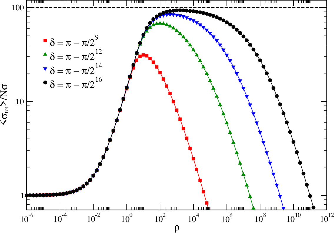
Refer to caption
Figure 1: Variation of the normalized mean cross section ⟨σtot⟩/N​σ{\left\langle{\sigma}_{\rm tot}\right\rangle}/\hskip 0.85355pt{\rm N}{\sigma} with the density ρ{\rho} of the samples for a set of values of the phase shift.
Refer to caption
Figure 2: Variation of the normalized mean cross section ⟨σtot⟩/N​σ{\left\langle{\sigma}_{\rm tot}\right\rangle}/\hskip 0.85355pt{\rm N}{\sigma} with the density ρ{\rho} of the samples for another set of values of the phase shift. The chosen number of scatterers is shown by an horizontal dashed line.

The obtained curves have a common feature, namely that the value of the normalized mean cross section is close to 11 when the density is very small, and so the radius very large. This is a consequence of the fact that the distance between the closest scatterers is sufficiently large in a typical arrangement of very low density for the contribution of a single scattering to be the largest one and so for the cross section to be almost equal to N​σ{\rm N}{\sigma}. The figures show also that the mean cross section first either decreases (Fig. 1) or increases (in the two figures) as the density increases; moreover, it always decreases uniformly as the density increases further on. The detailed explanation for each one of these two, less expected features of the mean cross section is given in the remainder of the section.

The decrease and the increase are both originated by double scattering; the reason for which the mean cross section can first deviate from N​σ{\rm N}{\sigma} in opposite ways is provided by its expression in the approximation of single and double scattering. This expression is derived in Appendix A. The result is

⟨σs+d⟩=N​σ+9​N​(N−1)4​(k​R)6​[sin⁡(2​δ)​C​(k​R)+cos⁡(2​δ)​S​(k​R)]​σ,\displaystyle{\left\langle{\sigma}_{{\rm s}+{\rm d}}\right\rangle}={\rm N}{\sigma}+\frac{9{\rm N}({\rm N}-1)}{4(k{\rm R})^{6}}\biggl[\hskip 0.68292pt\sin(2{\delta})\hskip 1.70709pt{\rm C}(k{\rm R})+\cos\hskip 0.62604pt(2{\delta})\,{\rm S}(k{\rm R})\hskip-0.31302pt\biggr]{\sigma}, (5.1)

(the subscript ”tot” has been replaced by ”s+d”, which is an abbreviation for ”s(ingle) and d(ouble scattering)”, in order to avoid any confusion with the exact cross section), with

C⁡(k​R)=(k​R)​cos⁡(4​k​R)16−sin⁡(4​k​R)64+(k​R)33{\rm C}(k{\rm R})=\frac{(k{\rm R})\cos\hskip 0.62604pt(4k{\rm R})}{16}-\frac{\sin(4k{\rm R})}{64}+\frac{(k{\rm R})^{3}}{3} (5.2)

and

S⁡(k​R)=(k​R)​sin⁡(4​k​R)16+cos⁡(4​k​R)64+(k​R)42−(k​R)28−164.{\rm S}(k{\rm R})=\frac{(k{\rm R})\sin(4k{\rm R})}{16}+\frac{\cos\hskip 0.62604pt(4k{\rm R})}{64}+\frac{(k{\rm R})^{4}}{2}-\frac{(k{\rm R})^{2}}{8}-\frac{1}{64}. (5.3)

When the radius is large enough, and so the density small enough, the contribution of double scattering is dominated by its term of least power, which is the one in 1/(k​R)21/(k{\rm R})^{2}. The normalized mean cross section is then well approximated by

⟨σtot⟩/N​σ\displaystyle{\left\langle{\sigma}_{\rm tot}\right\rangle}/{\rm N}{\sigma} =1+98​(N−1)​cos⁡(2​δ)(k​R)2\displaystyle=1+\frac{9}{8}({\rm N}-1)\,\frac{\cos\hskip 0.62604pt(2{\delta})}{(k{\rm R})^{2}} (5.4)
=1+12​(N−1)​cos⁡(2​δ)​(9​π​ρ2​N​k3)23.\displaystyle=1+\frac{1}{2}({\rm N}-1)\cos\hskip 0.62604pt(2{\delta})\biggl(\frac{9{\pi}{\rho}}{2{\rm N}k^{3}}\biggr)^{\hskip-2.16252pt\frac{2}{3}}.

This equation shows that if the phase shift takes on its values in ]π/4,3​π/4[]{\pi}/4\,,3{\pi}/4[, the contribution of double scattering is less than 00, which implies that the mean cross section decreases as the density increases (Fig. 1); on the contrary, if the phase shift takes on its values either in ]0,π/4[]0\,,{\pi}/4[ or ]3​π/4,π[]3{\pi}/4\,,{\pi}[, this contribution is greater than 00, with the consequence that the mean cross section increases as the density increases (in the two figures).

The fact that both the increase and the decrease are caused by double scattering alone is illustrated by the next two figures, in which the variation of ⟨σtot⟩{\left\langle{\sigma}_{\rm tot}\right\rangle} is compared to that of ⟨σs+d⟩{\left\langle{\sigma}_{{\rm s}+{\rm d}}\right\rangle} for two different values of the phase shift, one belonging to the interval ]π/4,3​π/4[]{\pi}/4\,,3{\pi}/4[ (Fig. 3) and the other to the interval ]3​π/4,π[]3{\pi}/4\,,{\pi}[ (Fig. 4). One sees that ⟨σtot⟩{\left\langle{\sigma}_{\rm tot}\right\rangle} has the same behaviour as ⟨σs+d⟩{\left\langle{\sigma}_{{\rm s}+{\rm d}}\right\rangle}, deviating from N{\rm N} by decreasing when δ{\delta} belongs to ]π/4,3​π/4[]{\pi}/4\,,3{\pi}/4[ and increasing when it belongs to ]3​π/4,π[]3{\pi}/4\,,{\pi}[, in agreement with (5.4). In addition, Fig. 4 shows that the mean cross section is not bounded in the approximation of single and double scattering, which comes from the fact that the ratio C⁡(k​R)/(k​R)6{\rm C}(k{\rm R})/(k{\rm R})^{6} diverges when the radius becomes arbitrarily small.

Refer to caption
Figure 3: Comparison of the variations of ⟨σtot⟩/N​σ{\left\langle{\sigma}_{\rm tot}\right\rangle}/{{\rm N}{\sigma}} and ⟨σs+d⟩/N​σ{\left\langle{\sigma}_{{\rm s}+{\rm d}}\right\rangle}/{{\rm N}{\sigma}} with the density ρ{\rho} of the samples for a value of the phase shift belonging to the interval ]π/4,3​π/4[]{\pi}/4\,,3{\pi}/4[.
Refer to caption
Figure 4: Comparison of the variations of ⟨σtot⟩/N​σ{\left\langle{\sigma}_{\rm tot}\right\rangle}/{{\rm N}{\sigma}} and ⟨σs+d⟩/N​σ{\left\langle{\sigma}_{{\rm s}+{\rm d}}\right\rangle}/{{\rm N}{\sigma}} with the density ρ{\rho} of the samples for a value of the phase shift belonging to the interval ]3​π/4,π[]3{\pi}/4\,,{\pi}[.

The uniform decrease of the mean cross section is caused by an unlimited number of contributions of successive scatterings to the cross section, that is to say, by multiple scattering. The expression of the mean cross section corresponding to an unlimited number of contributions of successive scatterings is derived in detail in Appendix B. We find

(k24​π)​(N−1N)​⟨σtot⟩\displaystyle\Biggl(\frac{k^{2}}{4\pi}\Biggr)\Biggl(\frac{{{\rm N}-1}}{{\rm N}}\Biggr){\left\langle{\sigma}_{\rm tot}\right\rangle}
=∑l=0∞(2​l+1)​Im{i⁡[(𝒦​R)​jl​(k​R)​jl+1​(𝒦​R)−(k​R)​jl​(𝒦​R)​jl+1​(k​R)(𝒦​R)​hl(1)​(k​R)​jl+1​(𝒦​R)−(k​R)​jl​(𝒦​R)​hl+1(1)​(k​R)]},\displaystyle=\sum_{l=0}^{\infty}(2l+1)\,\mathop{{\rm Im}}\Biggl\{i\Biggl[\frac{({\cal K}{\rm R})\,j_{l}(k{\rm R})\,j_{l+1}({\cal K}{\rm R})-(k{\rm R})\,j_{l}({\cal K}{\rm R})\,j_{l+1}(k{\rm R})}{({\cal K}{\rm R})\,h_{l}^{(1)}(k{\rm R})\,j_{l+1}({\cal K}{\rm R})-(k{\rm R})\,j_{l}({\cal K}{\rm R})\,h_{l+1}^{(1)}(k{\rm R})}\Biggr]\Biggr\},
(5.5)

with

𝒦=k​1+3​(N−1)​sin⁡δ​ei​δ(k​R)3.{\cal K}=k\,\sqrt{1+\frac{3({\rm N}-1)\sin\hskip-0.99594pt{\delta}\,{\rm e}^{\,i{\delta}}}{(k{\rm R})^{3}}}. (5.6)

In Figures 5 and 6 the mean cross section is compared to the curve obtained from the expression in (5.5), in which the sum has been truncated at l=150l=150, for the values of the phase shift that have been taken in the two previous figures.

Refer to caption
Figure 5: Comparison of the variations of the normalized mean cross section and of the expression of ⟨σtot⟩/N​σ{\left\langle{\sigma}_{\rm tot}\right\rangle}/{{\rm N}{\sigma}} given by (5.5), in which the sum has been truncated at l=150l=150 (dashed line), for a value of the phase shift belonging to the interval ]π/4,3​π/4[]{\pi}/4\,,3{\pi}/4[. The full line gives the values of the normalized cross section for diffusion by a hard sphere of radius R{\rm R}.

Each figure shows that the expression in (5.5) reproduces well the mean cross section except in the uninteresting range of values of the density in which the approximation of single scattering is valid. This discrepancy reflects the fact that the contributions of more and more partial waves have to be taken into account in the sum as the radius increases, and so as the density decreases. One can therefore conclude that the uniform decrease is caused by multiple scattering.

It is interesting to derive the expression to which (5.5) reduces when R{\rm R} tends to 0. We find

⟨σtot⟩≈4​πk2​Im{j0​(k​R)​(k​R)​ei​k​R}≈4​π​R2.\displaystyle{\left\langle{\sigma}_{\rm tot}\right\rangle}\approx\frac{4\pi}{k^{2}}\mathop{{\rm Im}}\biggl\{j_{0}(k{\rm R})\,(k{\rm R})\,{\rm e}^{\,ik{\rm R}}\biggr\}\approx 4\pi{\rm R}^{2}. (5.7)

This means that when the value of the density becomes arbitrarily large, the mean cross section tends towards the cross section for diffusion by a hard sphere whose radius is the same as that of the target, a behaviour which is clearly observed in Figures 5 and 6.

Refer to caption
Figure 6: Comparison of the variations of the normalized mean cross section and of the expression of ⟨σtot⟩/N​σ{\left\langle{\sigma}_{\rm tot}\right\rangle}/{{\rm N}{\sigma}} given by (5.5), in which the sum has been truncated at l=150l=150 (dashed line), for a value of the phase shift belonging to the interval ]3​π/4,π[]3{\pi}/4\,,{\pi}[. The full line gives the values of the normalized cross section for diffusion by a hard sphere of radius R{\rm R}.

6 Summary

In this paper, we have developed a formalism which describes the quantum scattering of a particle by a disordered target consisting of pointlike scatterers. The formalism has the important feature of preserving unitary because it takes into account all sequences of multiple scattering. We have used it in a numerical study about the scattering by a disordered target modelled by a set of pointlike scatterers which have each an equal probability of being at any position inside a sphere whose radius may be modified. We have studied the variation of the mean cross section with the density of the samples, and so with the radius of the target, for different values of the phase shift. The study has shown that the mean cross section goes through successive stages as the density increases, and so as the radius decreases. The mean cross section is nearly constant at very low density, which reflects the fact that the particle is only scattered once before leaving the target. Depending on the value of the phase shift, the mean cross section either increases or decreases as the density increases, each one of the two behaviours being originated by double scattering. As the density increases further on, the mean cross section decreases uniformly whatever the value of the phase shift, a behaviour which is caused by multiple scattering and which follows that of the cross section for diffusion by a hard sphere potential of decreasing radius.

Appendix A: Expression of the mean cross section in the approximation of single and double scattering

This appendix is devoted to the derivation of the expression of the mean cross section that includes only the contributions of single and double (m = 22) scattering. It follows from (4.7) that the mean cross section is given in this particular approximation by

⟨σs+d⟩=N​σ+σ​Im{e 2​i​δ​∑r=1N∑s=1(s≠r)N⟨(ei​k​Rr​sk​Rr​s)​ei​k→.R→r​s⟩}\displaystyle{\left\langle{\sigma}_{{\rm s}+{\rm d}}\right\rangle}={\rm N}{\sigma}+{\sigma}\hskip-0.42677pt\mathop{{\rm Im}}\Biggl\{{\rm e}^{\,2i{\delta}}\sum_{r=1}^{\rm N}\hskip-3.1298pt\sum_{\scriptstyle s=1\atop\scriptstyle(s\neq r)}^{\rm N}\hskip-3.1298pt{\left\langle\Biggl(\frac{{\rm e}^{\,ikR_{rs}}}{kR_{rs}}\Biggr)\,{\rm e}^{\,i{\vec{k}}.{\vec{R}}_{rs}}\right\rangle}\Biggr\} (A.1)

(the subscript is for ”s(ingle) and d(ouble scattering)”); finding its expression amounts therefore to hardly more than finding that of the mean of (ei​k​Rr​s/k​Rr​s)​ei​k→.R→r​s{({{\rm e}^{\,ikR_{rs}}}/{kR_{rs}})\,{\rm e}^{\,i{\vec{k}}.{\vec{R}}_{rs}}}.

Since each scatterer has an equal probability of being at any position in the target (whose center is taken as the origin of coordinates), we have

⟨(ei​k​Rr​sk​Rr​s)​ei​k→.R→r​s⟩\displaystyle{\left\langle\Biggl(\frac{{\rm e}^{\,ikR_{rs}}}{kR_{rs}}\Biggr)\,{\rm e}^{\,i{\vec{k}}.{\vec{R}}_{rs}}\right\rangle} =1V2​∫Vd​R→r​∫Vd​R→s​ei​k​Rr​s​ei​k→.R→r​sk​Rr​s\displaystyle=\frac{1}{{\rm V}^{2}}\int_{\rm V}{{\rm d}{\vec{R}}_{r}}\int_{\rm V}{{\rm d}{\vec{R}}_{s}}\,\frac{{\rm e}^{\,ikR_{rs}}\,{\rm e}^{\,i{\vec{k}}.{\vec{R}}_{rs}}}{kR_{rs}} (A.2)
=14​π​14​π​9R6​∫Vd​R→r​∫Vd​R→s​ei​k​Rr​s​ei​k→.R→r​sk​Rr​s.\displaystyle=\frac{1}{4\pi}\,\frac{1}{4\pi}\,\frac{9}{{\rm R}^{6}}\int_{\rm V}{{\rm d}{\vec{R}}_{r}}\int_{\rm V}{{\rm d}{\vec{R}}_{s}}\,\frac{{\rm e}^{\,ikR_{rs}}\,{\rm e}^{\,i{\vec{k}}.{\vec{R}}_{rs}}}{kR_{rs}}.

where V{\rm V} and R{\rm R} are the volume and radius of the target. The integration is most easily done working with the set of angular variables that consists of the azimuthal and polar angles Θr​s{\Theta}_{rs} and Φr​s{\Phi}_{rs} of the vector R→r​s{\vec{R}}_{rs}, the angle θr​s{\theta}_{rs} between the vectors R→r{\vec{R}}_{r} and R→s{\vec{R}}_{s}, and the angle ϕr​s{\phi}_{rs} between the planes that are defined by the vectors R→r{\vec{R}}_{r} and R→s{\vec{R}}_{s} and by the vectors R→r​s{\vec{R}}_{rs} and k→{\vec{k}} (which is assumed to determine the direction of the third axis). The expression of the product of volume elements for this choice of angular variables is

dR→rdR→s=R2rdRrR2sdRssinΘr​sdΘr​sdΦr​ssinθr​sdθr​sdϕr​s,{{\rm d}{\vec{R}}_{r}}\hskip 1.13791pt{{\rm d}{\vec{R}}_{s}}={R^{2}_{r}}\hskip 1.13791pt{{\rm d}R_{r}}\hskip 0.56917pt{R^{2}_{s}}\hskip 1.13791pt{{\rm d}R_{s}}\hskip 2.13387pt{\sin\hskip-1.28032pt{\Theta}_{rs}}\hskip 1.13791pt{{\rm d}{\Theta}_{rs}}\hskip 1.13791pt{{\rm d}{\Phi}_{rs}}\hskip 2.13387pt{\sin\hskip-0.99594pt{\theta}_{rs}}\hskip 1.13791pt{{\rm d}{\theta}_{rs}}\hskip 1.13791pt{{\rm d}{\phi}_{rs}}, (A.3)

where Rr⁡(s)R_{r(s)} is the magnitude of the vector R→r⁡(s){\vec{R}}_{r(s)}.

The expression of the mean of (ei​k​Rr​s/k​Rr​s)​ei​k→.R→r​s{({{\rm e}^{\,ikR_{rs}}}/{kR_{rs}})\,{\rm e}^{\,i{\vec{k}}.{\vec{R}}_{rs}}} may be obtained by successive averages over pairs of variables; the variables with respect to which the integration has been done will be indicated in a subscript. The average over Θr​s{\Theta}_{rs} and Φr​s{\Phi}_{rs} gives

⟨(ei​k​Rr​sk​Rr​s)​ei​k→.R→r​s⟩(Θr​s,Φr​s)\displaystyle{\left\langle\Biggl(\frac{{\rm e}^{\,ikR_{rs}}}{kR_{rs}}\Biggr)\,{\rm e}^{\,i{\vec{k}}.{\vec{R}}_{rs}}\right\rangle}_{({\Theta}_{rs},{\Phi}_{rs})}
=14​πei​k​Rr​sk​Rr​s∫0πsinΘr​sdΘr​s∫02​πdΦr​seikRr​scosΘr​s\displaystyle=\frac{1}{4\pi}\,\frac{{\rm e}^{\,ikR_{rs}}}{kR_{rs}}\int_{0}^{\pi}{\sin\hskip-1.28032pt{\Theta}_{rs}}\hskip 1.13791pt{{\rm d}{\Theta}_{rs}}\int_{0}^{2\pi}{{\rm d}{\Phi}_{rs}}\,{\rm e}^{\,ikR_{rs}\hskip-0.45541pt\cos\hskip-0.5123pt{\Theta}_{rs}}
=∑n=0∞(2​i)n(n+1)!​(k​Rr​s)n−1.\displaystyle=\sum_{n=0}^{\infty}\frac{(2i)^{n}}{(n+1)!}(kR_{rs})^{n-1}. (A.4)

It follows that

⟨(ei​k​Rr​sk​Rr​s)​ei​k→.R→r​s⟩=∑n=0∞(2​i)n(n+1)!​⟨(k​Rr​s)n−1⟩(θr​s,ϕr​s,Rr,Rs),\displaystyle{\left\langle\biggl(\frac{{\rm e}^{\,ikR_{rs}}}{kR_{rs}}\biggr)\,{\rm e}^{\,i{\vec{k}}.{\vec{R}}_{rs}}\right\rangle}=\sum_{n=0}^{\infty}\frac{(2i)^{n}}{(n+1)!}\,{\left\langle(kR_{rs})^{n-1}\right\rangle}_{({\theta}_{rs},{\phi}_{rs};R_{r},R_{s})}, (A.5)

and so we need the expression of the mean of (k​Rr​s)n−1(kR_{rs})^{n-1} for any nn to obtain that of the mean of (ei​k​Rr​s/k​Rr​s)​ei​k→.R→r​s{({{\rm e}^{\,ikR_{rs}}}/{kR_{rs}})\,{\rm e}^{\,i{\vec{k}}.{\vec{R}}_{rs}}}.

The average of (k​Rr​s)n−1(kR_{rs})^{n-1} over the angles gives

⟨(k​Rr​s)n−1⟩(θr​s,ϕr​s)\displaystyle{\left\langle(kR_{rs})^{n-1}\right\rangle}_{({\theta}_{rs},{\phi}_{rs})}
=kn−14​π∫0πsinθr​sdθr​s∫02​πdϕr​s(Rr2+Rs2−2RrRscosθr​s)n−12\displaystyle=\frac{k^{n-1}}{4\pi}\int_{0}^{\pi}{\sin\hskip-0.99594pt{\theta}_{rs}}\hskip 1.13791pt{{\rm d}{\theta}_{rs}}\int_{0}^{2\pi}{{\rm d}{\phi}_{rs}}\,(R^{2}_{r}+R^{2}_{s}-2R_{r}R_{s}\cos\hskip-0.36685pt{\theta}_{rs})^{\hskip-0.768pt\frac{n-1}{2}}
=kn−12​(n+1)((Rr+Rs)n+1−|Rr−Rs|n+1Rr​Rs)(n=0,1,…).\displaystyle=\frac{k^{n-1}}{2(n+1)}\hskip 0.71114pt\Biggl(\frac{(R_{r}+R_{s})^{n+1}-|R_{r}-R_{s}|^{n+1}}{R_{r}R_{s}}\Biggr)\,\,\,\,\,\,\,\,\,\,\,\,\,\,\,\,\,(n=0,1,...). (A.6)

The average of the obtained expression gives that of the mean of (k​Rr​s)n−1(kR_{rs})^{n-1}. We find

⟨(k​Rr​s)n−1⟩(θr​s,ϕr​s,Rr,Rs)\displaystyle{\left\langle(kR_{rs})^{n-1}\right\rangle}_{({\theta}_{rs},{\phi}_{rs};R_{r},R_{s})}
=⟨kn−12​(n+1)​((Rr+Rs)n+1−|Rr−Rs|n+1Rr​Rs)⟩(Rr,Rs)\displaystyle={\left\langle\frac{k^{n-1}}{2(n+1)}\hskip 0.71114pt\Biggl(\frac{(R_{r}+R_{s})^{n+1}-|R_{r}-R_{s}|^{n+1}}{R_{r}R_{s}}\Biggr)\right\rangle}_{(R_{r},R_{s})}
=9R6​kn−12​(n+1)​∫0RRr​d​Rr​∫0RRs​d​Rs​[(Rr+Rs)n+1−|Rr−Rs|n+1]\displaystyle=\frac{9}{{\rm R}^{6}}\,\frac{k^{n-1}}{2(n+1)}\int_{0}^{\rm R}{R_{r}}\hskip 1.13791pt{{\rm d}R_{r}}\int_{0}^{\rm R}{R_{s}}\hskip 1.13791pt{{\rm d}R_{s}}\,[(R_{r}+R_{s})^{n+1}-|R_{r}-R_{s}|^{n+1}\hskip-0.28436pt]
=72​(2​k​R)n−1(n+2)​(n+3)​(n+5)(n=0,1,…).\displaystyle=\frac{72\,(2k{\rm R})^{n-1}}{(n+2)(n+3)(n+5)}\,\,\,\,\,\,\,\,\,\,\,\,\,\,\,\,\,\,\,\,\,\,\,\,\,\,\,\,\,\,\,\,\,\,\,\,\,\,\,\,\,\,\,\,\,\,\,\,\,\,\,\,\,\,\,\,\,\,\,\,\,\,\,\,\,\,(n=0,1,...). (A.7)

Substituting the expression of the mean of (k​Rr​s)n−1(kR_{rs})^{n-1} into (A.5), we obtain

⟨(ei​k​Rr​sk​Rr​s)​ei​k→.R→r​s⟩\displaystyle{\left\langle\Biggl(\frac{{\rm e}^{\,ikR_{rs}}}{kR_{rs}}\Biggr)\,{\rm e}^{\,i{\vec{k}}.{\vec{R}}_{rs}}\right\rangle}
=722​k​R​∑n=0∞(4​i​k​R)n(n+1)!​(n+2)​(n+3)​(n+5)\displaystyle=\frac{72}{2k{\rm R}}\sum_{n=0}^{\infty}\frac{(4ik{\rm R})^{n}}{(n+1)!(n+2)(n+3)(n+5)}
=144(4​k​R)5​[e 4​i​k​R−1−4​i​k​R−(4​i​k​R)22−(4​i​k​R)36]\displaystyle=\frac{144}{(4k{\rm R})^{5}}\biggl[\hskip 0.68292pt{\rm e}^{\,4ik{\rm R}}-1-4ik{\rm R}-\frac{(4ik{\rm R})^{2}}{2}-\frac{(4ik{\rm R})^{3}}{6}\biggr]
+i​144(4​k​R)6​[e 4​i​k​R−1−4​i​k​R−(4​i​k​R)22−(4​i​k​R)36−(4​i​k​R)424].\displaystyle\,\,\,+i\frac{144}{(4k{\rm R})^{6}}\biggl[\hskip 0.68292pt{\rm e}^{\,4ik{\rm R}}-1-4ik{\rm R}-\frac{(4ik{\rm R})^{2}}{2}-\frac{(4ik{\rm R})^{3}}{6}-\frac{(4ik{\rm R})^{4}}{24}\biggr]. (A.8)

Substitution of the expression of the mean of (ei​k​Rr​s/k​Rr​s)​ei​k→.R→r​s({\rm e}^{\,ikR_{rs}}/{kR_{rs}})\,{\rm e}^{\,i{\vec{k}}.{\vec{R}}_{rs}} into (A.1) leads to that of the mean cross section in the approximation of single and double scattering, which is

⟨σs+d⟩=N​σ+9​N​(N−1)4​(k​R)6​[sin⁡(2​δ)​C​(k​R)+cos⁡(2​δ)​S​(k​R)]​σ,\displaystyle{\left\langle{\sigma}_{{\rm s}+{\rm d}}\right\rangle}={\rm N}{\sigma}+\frac{9{\rm N}({\rm N}-1)}{4(k{\rm R})^{6}}\biggl[\hskip 0.68292pt\sin(2{\delta})\hskip 1.70709pt{\rm C}(k{\rm R})+\cos\hskip 0.62604pt(2{\delta})\,{\rm S}(k{\rm R})\hskip-0.31302pt\biggr]{\sigma}, (A.9)

with

C⁡(k​R)=(k​R)​cos⁡(4​k​R)16−sin⁡(4​k​R)64+(k​R)33{\rm C}(k{\rm R})=\frac{(k{\rm R})\cos\hskip 0.62604pt(4k{\rm R})}{16}-\frac{\sin(4k{\rm R})}{64}+\frac{(k{\rm R})^{3}}{3} (A.10)

and

S⁡(k​R)=(k​R)​sin⁡(4​k​R)16+cos⁡(4​k​R)64+(k​R)42−(k​R)28−164.{\rm S}(k{\rm R})=\frac{(k{\rm R})\sin(4k{\rm R})}{16}+\frac{\cos\hskip 0.62604pt(4k{\rm R})}{64}+\frac{(k{\rm R})^{4}}{2}-\frac{(k{\rm R})^{2}}{8}-\frac{1}{64}. (A.11)

The functions C⁡(k​R){\rm C}(k{\rm R}) and S⁡(k​R){\rm S}(k{\rm R}) take on only positive values. It is to be noted that the mean cross section is not bounded in the approximation of single and double scattering because the function C⁡(k​R)/(k​R)6{\rm C}(k{\rm R})/(k{\rm R})^{6} behaves like 1/k​R1/k{\rm R} when R{\rm R} tends to 00.

Appendix B: Expression of the mean cross section for an unlimited number of contributions of successive scatterings

This appendix is devoted to the derivation of the expression of the mean cross section for an unlimited number of contributions of successive scatterings to the cross section. The relevant expression for the cross section is obtained from (4.7) by discarding the remainder term and letting the integer M{\rm M} become infinitely large. The formula giving the mean cross section is then

⟨σtot⟩\displaystyle{\left\langle{\sigma}_{\rm tot}\right\rangle} =N​σ\displaystyle={\rm N}{\sigma} (B.1)
+4​πk2∑m=2M(sinδ)mIm{ei​m​δ∑r1=1N∑r2=1(r2≠r1)N…∑rm=1(rm≠rm−1)N⟨(ei​k​Rr1​r2k​Rr1​r2)\displaystyle\,\,\,+\frac{4\pi}{k^{2}}\sum_{{\rm m}=2}^{\rm M}\,(\sin\hskip-0.99594pt{\delta})^{\rm m}\hskip 0.28436pt\mathop{{\rm Im}}\Biggl\{{\rm e}^{\,i{\rm m}{\delta}}\sum_{r_{1}\hskip-0.42677pt=1}^{\rm N}\hskip-3.1298pt\sum_{\scriptstyle r_{2}=1\atop\scriptstyle(r_{2}\neq r_{1}\hskip-0.42677pt)}^{\rm N}\dots\sum_{\scriptstyle r_{\rm m}=1\atop\scriptstyle(r_{\rm m}\neq r_{{\rm m}-1}\hskip-0.42677pt)}^{\rm N}\hskip-3.1298pt\Biggl\langle\Biggl(\frac{{\rm e}^{\,ikR_{r_{1}\hskip-0.71114ptr_{2}}}}{kR_{r_{1}\hskip-0.71114ptr_{2}}}\Biggr)
×(ei​k​Rr2​r3k​Rr2​r3)…(ei​k​Rrm−1​rmk​Rrm−1​rm)ei​k→.R→r1​rm⟩},\displaystyle\,\,\,\,\,\,\,\,\times\Biggl(\frac{{\rm e}^{\,ikR_{r_{2}r_{3}}}}{kR_{r_{2}r_{3}}}\Biggr)\dots\Biggl(\frac{{\rm e}^{\,ikR_{r_{{\rm m}-1}\hskip-0.71114ptr_{\rm m}}}}{kR_{r_{{\rm m}-1}\hskip-0.71114ptr_{\rm m}}}\Biggr)\,{\rm e}^{\,i{\vec{k}}.{\vec{R}}_{r_{1}\hskip-0.71114ptr_{\rm m}}}\hskip-1.9919pt\Biggr\rangle\Biggr\},

where M{\rm M} is as large as desired. Since σ=(4​π/k2)​sin2⁡δ{\sigma}=(4{\pi}/k^{2})\sin^{2}\hskip-1.28032pt{\delta}, this formula may be written as

⟨σtot⟩=4​πk2​N​∑m=1M(N−1)m−1​(sin⁡δ)m​Im{ei​m​δ​Mm​(k​R)},\displaystyle{\left\langle{\sigma}_{\rm tot}\right\rangle}=\frac{4\pi}{k^{2}}\hskip 0.99594pt{\rm N}\sum_{{\rm m}=1}^{\rm M}\,({\rm N}-1)^{{\rm m}-1}(\sin\hskip-0.99594pt{\delta})^{\rm m}\hskip 0.28436pt\mathop{{\rm Im}}\biggl\{{\rm e}^{\,i{\rm m}{\delta}}M_{\rm m}(k{\rm R})\biggr\}, (B.2)

with

M1​(k​R)=1M_{1}(k{\rm R})=1 (B.3)

and

Mm​(k​R)\displaystyle M_{\rm m}(k{\rm R}) =1N​(N−1)m−1[∑r1=1N∑r2=1(r2≠r1)N…∑rm=1(rm≠rm−1)N⟨(ei​k​Rr1​r2k​Rr1​r2)\displaystyle=\frac{1}{{\rm N}({\rm N}-1)^{{\rm m}-1}}\Biggl[\,\sum_{r_{1}\hskip-0.42677pt=1}^{\rm N}\hskip-3.1298pt\sum_{\scriptstyle r_{2}=1\atop\scriptstyle(r_{2}\neq r_{1}\hskip-0.42677pt)}^{\rm N}\dots\sum_{\scriptstyle r_{\rm m}=1\atop\scriptstyle(r_{\rm m}\neq r_{{\rm m}-1}\hskip-0.42677pt)}^{\rm N}\hskip-3.1298pt\Biggl\langle\Biggl(\frac{{\rm e}^{\,ikR_{r_{1}\hskip-0.71114ptr_{2}}}}{kR_{r_{1}\hskip-0.71114ptr_{2}}}\Biggr) (B.4)
×(ei​k​Rr2​r3k​Rr2​r3)…(ei​k​Rrm−1​rmk​Rrm−1​rm)ei​k→.R→r1​rm⟩]\displaystyle\,\,\,\,\,\,\,\,\,\,\,\,\,\,\,\,\,\,\,\,\,\,\,\,\,\,\,\,\,\,\,\,\,\,\,\times\Biggl(\frac{{\rm e}^{\,ikR_{r_{2}r_{3}}}}{kR_{r_{2}r_{3}}}\Biggr)\dots\Biggl(\frac{{\rm e}^{\,ikR_{r_{{\rm m}-1}\hskip-0.71114ptr_{\rm m}}}}{kR_{r_{{\rm m}-1}\hskip-0.71114ptr_{\rm m}}}\Biggr)\,{\rm e}^{\,i{\vec{k}}.{\vec{R}}_{r_{1}\hskip-0.71114ptr_{\rm m}}}\hskip-1.9919pt\Biggr\rangle\Biggr]
(m=2,3,…).\displaystyle\,\,\,\,\,\,\,\,\,\,\,\,\,\,\,\,\,\,\,\,\,\,\,\,\,\,\,\,\,\,\,\,\,\,\,\,\,\,\,\,\,\,\,\,\,\,\,\,\,\,\,\,\,\,\,\,\,\,\,\,\,\,\,\,\,\,\,\,\,\,\,\,\,\,\,\,\,\,\,\,\,\,\,\,\,\,\,\,\,\,\,\,\,\,\,\,\,\,\,\,\,\,\,\,\,\,\,({\rm m}=2,3\hskip 0.42677pt,...).

Since each scatterer has an equal probability of being at any position inside a sphere of volume V{\rm V} and radius R{\rm R} (whose center is taken as the origin of coordinates), we have

Mm​(k​R)\displaystyle M_{\rm m}(k{\rm R}) =1Vm​∫Vd​R→1​∫Vd​R→2​…​∫Vd​R→m​(ei​k​R12k​R12)\displaystyle=\frac{1}{{\rm V}^{\rm m}}\int_{{\rm V}}{{\rm d}{\vec{R}}_{1}}\int_{{\rm V}}{{\rm d}{\vec{R}}_{2}}\dots\int_{{\rm V}}{{\rm d}{\vec{R}}_{\rm m}}\,\Biggl(\frac{{\rm e}^{\,ikR_{12}}}{kR_{12}}\Biggr) (B.5)
×(ei​k​R23k​R23)​…​(ei​k​Rm−1​mk​Rm−1​m)​e−i​k→.R→1​ei​k→.R→m\displaystyle\,\,\,\,\,\,\,\,\times\Biggl(\frac{{\rm e}^{\,ikR_{23}}}{kR_{23}}\Biggr)\dots\Biggl(\frac{{\rm e}^{\,ikR_{{{\rm m}-1}{\rm m}}}}{kR_{{{\rm m}-1}{\rm m}}}\Biggr)\,{\rm e}^{\,-i{\vec{k}}.{\vec{R}}_{1}}\,{\rm e}^{\,i{\vec{k}}.{\vec{R}}_{\rm m}}
(m=2,3,…).\displaystyle\,\,\,\,\,\,\,\,\,\,\,\,\,\,\,\,\,\,\,\,\,\,\,\,\,\,\,\,\,\,\,\,\,\,\,\,\,\,\,\,\,\,\,\,\,\,\,\,\,\,\,\,\,\,\,\,\,\,\,\,\,\,\,\,\,\,\,\,\,\,\,\,\,\,\,\,\,\,\,\,\,\,\,\,\,\,\,\,\,\,\,\,\,\,\,\,\,\,\,\,\,\,\,\,\,\,\,({\rm m}=2,3,...).

Introducing the reduced vectors

u→i=R→i/R(i=1,2,…),{\vec{u}}_{i}={{\vec{R}}_{i}}/\hskip 0.1424pt{\rm R}\,\,\,\,\,\,\,\,\,\,\,\,\,\,\,\,\,\,\,\,\,\,\,\,\,\,\,\,\,\,\,\,\,\,\,\,\,\,\,\,\,\,\,\,\,\,\,\,\,\,\,\,\,\,\,\,\,\,\,\,\,\,\,\,\,\,\,\,\,\,\,\,\,\,\,\,\,\,\,\,\,\,\,\,\,\,\,\,\,\,\,\,\,\,\,\,\,\,\,\,\,\,\,\,\,(i=1\hskip-0.42677pt,2\hskip 0.42677pt,...), (B.6)

we may also write the expression of Mm​(k​R)M_{\rm m}(k{\rm R}) as

Mm​(k​R)\displaystyle M_{\rm m}(k{\rm R}) =3m(4​π)m​∫d​u→1​∫d​u→2​…​∫d​u→m​(ei​k​R​|u→2−u→1|k​R​|u→2−u→1|)\displaystyle=\frac{3^{\rm m}}{(4\pi)^{\rm m}}\int{{\rm d}{\vec{u}}_{1}}\int{{\rm d}{\vec{u}}_{2}}\dots\int{{\rm d}{\vec{u}}_{\rm m}}\,\Biggl(\frac{{\rm e}^{\,ik{\rm R}|{\vec{u}}_{2}-{\vec{u}}_{1}|}}{k{\rm R}|{\vec{u}}_{2}-{\vec{u}}_{1}|}\Biggr) (B.7)
×(ei​k​R​|u→3−u→2|k​R​|u→3−u→2|)​…​(ei​k​R​|u→m−u→m−1|k​R​|u→m−u→m−1|)​e−i​R​k→.u→1​ei​R​k→.u→m\displaystyle\,\,\,\,\,\,\,\,\times\Biggl(\frac{{\rm e}^{\,ik{\rm R}|{\vec{u}}_{3}-{\vec{u}}_{2}|}}{k{\rm R}|{\vec{u}}_{3}-{\vec{u}}_{2}|}\Biggr)\dots\Biggl(\frac{{\rm e}^{\,ik{\rm R}|{\vec{u}}_{\rm m}-{\vec{u}}_{{\rm m}-1}|}}{k{\rm R}|{\vec{u}}_{\rm m}-{\vec{u}}_{{\rm m}-1}|}\Biggr)\,{\rm e}^{\,-i{\rm R}{\vec{k}}.{\vec{u}}_{1}}\,{\rm e}^{\,i{\rm R}{\vec{k}}.{\vec{u}}_{\rm m}}
(m=2,3,…),\displaystyle\,\,\,\,\,\,\,\,\,\,\,\,\,\,\,\,\,\,\,\,\,\,\,\,\,\,\,\,\,\,\,\,\,\,\,\,\,\,\,\,\,\,\,\,\,\,\,\,\,\,\,\,\,\,\,\,\,\,\,\,\,\,\,\,\,\,\,\,\,\,\,\,\,\,\,\,\,\,\,\,\,\,\,\,\,\,\,\,\,\,\,\,\,\,\,\,\,\,\,\,\,\,\,\,\,\,\,({\rm m}=2,3,...),

where each integration is over all points inside a sphere of radius 1. The mean of the contribution of any number of successive scatterings may be written in the form

Mn+1​(k​R)=∫01d​u​𝒫n​(u,k​R)(n=0,1,…)M_{{\rm n}+1}(k{\rm R})=\int_{0}^{1}{{\rm d}u}\,{\cal P}_{\rm n}(u,k{\rm R})\,\,\,\,\,\,\,\,\,\,\,\,\,\,\,\,\,\,\,\,\,\,\,\,\,\,\,\,\,\,\,\,\,\,\,\,\,\,\,\,\,\,\,\,\,\,\,\,\,\,\,\,\,\,\,\,({\rm n}=0,1,...) (B.8)

with

𝒫0​(u,k​R)=3​u2,{\cal P}_{0}(u,k{\rm R})=3\,u^{2}, (B.9)
𝒫1​(u,k​R)=3​u2​3(4​π)2​∫d​Ωu→​ei​R​k→.u→​∫d​r→1​e−i​R​k→.u→1​(ei​k​R​|u→−u→1|k​R​|u→−u→1|),{\cal P}_{1}(u,k{\rm R})=3u^{2}\frac{3}{(4\pi)^{2}}\int{{\rm d}{\Omega}_{\vec{u}}}\,{\rm e}^{\,i{\rm R}{\vec{k}}.{\vec{u}}}\int{{\rm d}{\vec{r}}_{1}}\,{\rm e}^{\,-i{\rm R}{\vec{k}}.{\vec{u}}_{1}}\Biggl(\frac{{\rm e}^{\,ik{\rm R}|{\vec{u}}-{\vec{u}}_{1}\hskip-0.42677pt|}}{k{\rm R}|{\vec{u}}-{\vec{u}}_{1}\hskip-0.71114pt|}\Biggr), (B.10)

and

𝒫n​(u,k​R)\displaystyle{\cal P}_{\rm n}(u,k{\rm R}) =3​u2​3n(4​π)n+1​∫d​Ωu→​∫d​u→1​∫d​u→2​…​∫d​u→n​(ei​k​R​|u→2−u→1|k​R​|u→2−u→1|)\displaystyle=3\,u^{2}\frac{3^{\rm n}}{(4\pi)^{{\rm n}+1}}\int{{\rm d}{\Omega}_{\vec{u}}}\int{{\rm d}{\vec{u}}_{1}}\int{{\rm d}{\vec{u}}_{2}}\dots\int{{\rm d}{\vec{u}}_{\rm n}}\,\Biggl(\frac{{\rm e}^{\,ik{\rm R}|{\vec{u}}_{2}-{\vec{u}}_{1}|}}{k{\rm R}|{\vec{u}}_{2}-{\vec{u}}_{1}|}\Biggr) (B.11)
×(ei​k​R​|u→3−u→2|k​R​|u→3−u→2|)​…​(ei​k​R​|u→n−u→n−1|k​R​|u→n−u→n−1|)​e−i​R​k→.u→1\displaystyle\,\,\,\,\,\,\,\,\times\Biggl(\frac{{\rm e}^{\,ik{\rm R}|{\vec{u}}_{3}-{\vec{u}}_{2}|}}{k{\rm R}|{\vec{u}}_{3}-{\vec{u}}_{2}|}\Biggr)\dots\Biggl(\frac{{\rm e}^{\,ik{\rm R}|{\vec{u}}_{\rm n}-{\vec{u}}_{{\rm n}-1}|}}{k{\rm R}|{\vec{u}}_{\rm n}-{\vec{u}}_{{\rm n}-1}|}\Biggr)\,{\rm e}^{\,-i{\rm R}{\vec{k}}.{\vec{u}}_{1}}
×(ei​k​R​|u→−u→n|k​R​|u→−u→n|)​ei​R​k→.u→\displaystyle\,\,\,\,\,\,\,\,\times\Biggl(\frac{{\rm e}^{\,ik{\rm R}|{\vec{u}}-{\vec{u}}_{\rm n}|}}{k{\rm R}|{\vec{u}}-{\vec{u}}_{\rm n}|}\Biggr)\,{\rm e}^{\,i{\rm R}{\vec{k}}.{\vec{u}}}
(n=2,3,…).\displaystyle\,\,\,\,\,\,\,\,\,\,\,\,\,\,\,\,\,\,\,\,\,\,\,\,\,\,\,\,\,\,\,\,\,\,\,\,\,\,\,\,\,\,\,\,\,\,\,\,\,\,\,\,\,\,\,\,\,\,\,\,\,\,\,\,\,\,\,\,\,\,\,\,\,\,\,\,\,\,\,\,\,\,\,\,\,\,\,\,\,\,\,\,\,\,\,\,\,\,\,\,\,\,\,({\rm n}=2,3,...).

The recursion formula for the quantities 𝒫n​(u,k​R){\cal P}_{\rm n}(u,k{\rm R}) is then obtained by substituting the expansions [11]

ei​k→.R→=4​π​∑l=0∞∑m=−llil​jl​(k​R)​Yl​m∗​(Ωk→)​Yl​m​(ΩR→),{\rm e}^{\,i{\vec{k}}.{\vec{R}}}={4\pi}\sum_{l=0}^{\infty}\sum_{m=-l}^{l}i^{l}\,j_{l}(kR)\,Y_{lm}^{*}({\Omega}_{{\vec{k}}})\,Y_{lm}({\Omega}_{{\vec{R}}}), (B.12)

where RR and ΩR→{\Omega}_{{\vec{R}}} are the magnitude and direction of the vector R→{\vec{R}}, and

ei​k​R​|u→s−u→r|k​R​|u→s−u→r|\displaystyle\frac{{\rm e}^{\,ik{\rm R}|{\vec{u}}_{s}-{\vec{u}}_{r}|}}{k{\rm R}|{\vec{u}}_{s}-{\vec{u}}_{r}|}
=4​π​i​∑l=0∞∑m=−lljl​(k​RMin​(ur,us))​hl(1)​(k​RMax​(ur,us))​Yl​m∗​(Ωu→r)​Yl​m​(Ωu→s)\displaystyle={4\pi}i\sum_{l=0}^{\infty}\sum_{m=-l}^{l}j_{l}(k{\rm R}{\rm Min}(u_{r},u_{s}))\,h_{l}^{(1)}(k{\rm R}{\rm Max}(u_{r},u_{s}))\,Y_{lm}^{*}({\Omega}_{{\vec{u}}_{r}})\,Y_{lm}({\Omega}_{{\vec{u}}_{s}})
(s≠r),\displaystyle\,\,\,\,\,\,\,\,\,\,\,\,\,\,\,\,\,\,\,\,\,\,\,\,\,\,\,\,\,\,\,\,\,\,\,\,\,\,\,\,\,\,\,\,\,\,\,\,\,\,\,\,\,\,\,\,\,\,\,\,\,\,\,\,\,\,\,\,\,\,\,\,\,\,\,\,\,\,\,\,\,\,\,\,\,\,\,\,\,\,\,\,\,\,\,\,\,\,\,\,\,\,\,\,\,\,\,\,\,\,\,\,\,\,\,\,\,\,\,\,\,\,\,\,\,\,\,\,\,\,\,\,\,\,\,\,\,\,\,\,\,(s\neq r), (B.13)

where ur⁡(s)u_{r(s)} and Ωu→r⁡(s){\Omega}_{{\vec{u}}_{r(s)}} are the magnitude and direction of the vector u→r⁡(s){\vec{u}}_{r(s)} and where Min⁡(ur,us){\rm Min}(u_{r},u_{s}) is the smaller and Max⁡(ur,us){\rm Max}(u_{r},u_{s}) the larger of uru_{r} and usu_{s}, into (B.11). Using the notations Ωu→r=Ωr{\Omega}_{{\vec{u}}_{r}}={\Omega}_{r} (r=1,…,n)(r=1,...,{\rm n}), we obtain

𝒫n​(u,k​R)\displaystyle{\cal P}_{\rm n}(u,k{\rm R}) =3​u2​(4​π)​in​∑l=0∞∑m=−llil​jl​(k​R)​Yl​m∗​(Ωk→)\displaystyle=3\,u^{2}\,(4\pi)\,i^{\rm n}\sum_{l=0}^{\infty}\sum_{m=-l}^{l}i^{l}\,j_{l}(k{\rm R})\,Y_{lm}^{*}({\Omega}_{{\vec{k}}})
∑l′=0∞∑m′=−l′l′(−i)l′Yl′​m′(Ωk→)∑l1=0∞∑m1=−l1l1∑l2=0∞∑m2=−l2l2…∑ln=0∞∑mn=−lnln\displaystyle\,\,\,\,\,\,\,\,\sum_{l^{\prime}=0}^{\infty}\sum_{m^{\prime}=-l^{\prime}}^{l^{\prime}}(-i)^{l^{\prime}}\,Y_{l^{\prime}m^{\prime}}({\Omega}_{{\vec{k}}})\sum_{l_{1}=0}^{\infty}\sum_{m_{1}=-l_{1}}^{l_{1}}\sum_{l_{2}=0}^{\infty}\sum_{m_{2}=-l_{2}}^{l_{2}}\dots\sum_{l_{\rm n}=0}^{\infty}\sum_{m_{\rm n}=-l_{\rm n}}^{l_{\rm n}}
×∫013​u12​d​u1​∫013​u22​d​u2​…​∫013​un2​d​un​jl1​(k​RMin​(u1,u2))\displaystyle\,\,\,\,\,\,\,\,\times\int_{0}^{1}\hskip-1.42271pt3\,u_{1}^{2}\hskip 0.28436pt{{\rm d}u_{1}}\int_{0}^{1}\hskip-1.42271pt3\,u_{2}^{2}\hskip 0.42677pt{{\rm d}u_{2}}\dots\int_{0}^{1}\hskip-1.42271pt3\,u_{\rm n}^{2}\hskip 0.56917pt{{\rm d}u_{\rm n}}\,j_{l_{1}}(k{\rm R}{\rm Min}(u_{1},u_{2}))\,
×hl1(1)​(k​RMax​(u1,u2))​jl2​(k​RMin​(u2,u3))\displaystyle\,\,\,\,\,\,\,\,\times h_{l_{1}}^{(1)}(k{\rm R}{\rm Max}(u_{1},u_{2}))\,j_{l_{2}}(k{\rm R}{\rm Min}(u_{2},u_{3}))\,
×hl2(1)​(k​RMax​(u2,u3))​…​jln−1​(k​RMin​(un−1,un))\displaystyle\,\,\,\,\,\,\,\,\times h_{l_{2}}^{(1)}(k{\rm R}{\rm Max}(u_{2},u_{3}))\dots j_{l_{{\rm n}-1}}(k{\rm R}{\rm Min}(u_{{\rm n}-1},u_{\rm n}))
×hln−1(1)​(k​RMax​(un−1,un))​jln​(k​RMin​(un,k​r))\displaystyle\,\,\,\,\,\,\,\,\times h_{l_{{\rm n}-1}}^{(1)}(k{\rm R}{\rm Max}(u_{{\rm n}-1},u_{\rm n}))\,j_{l_{\rm n}}(k{\rm R}{\rm Min}(u_{\rm n},kr))
×hln(1)​(k​RMax​(un,k​r))​jl′​(k​R​u1)​∫d​Ωr→​∫d​Ω1\displaystyle\,\,\,\,\,\,\,\,\times h_{l_{\rm n}}^{(1)}(k{\rm R}{\rm Max}(u_{\rm n},kr))\,j_{l^{\prime}}(k{\rm R}u_{1})\int\hskip-0.56917pt{{\rm d}{\Omega}_{\vec{r}}}\int\hskip-0.56917pt{{\rm d}{\Omega}_{1}}
×∫d​Ω2​…​∫d​Ωn​Yl1​m1∗​(Ω1)​Yl1​m1​(Ω2)\displaystyle\,\,\,\,\,\,\,\,\times\int\hskip-0.56917pt{{\rm d}{\Omega}_{2}}\dots\int\hskip-0.56917pt{{\rm d}{\Omega}_{\rm n}}\,Y_{l_{1}m_{1}}^{*}({\Omega}_{1})\,Y_{l_{1}m_{1}}({\Omega}_{2})\,
×Yl2​m2∗​(Ω2)​Yl2​m2​(Ω3)​…​Yln−1​mn−1∗​(Ωn−1)​Yln−1​mn−1​(Ωn)\displaystyle\,\,\,\,\,\,\,\,\times Y_{l_{2}m_{2}}^{*}({\Omega}_{2})\,Y_{l_{2}m_{2}}({\Omega}_{3})\dots Y_{l_{{\rm n}-1}m_{{\rm n}-1}}^{*}({\Omega}_{{\rm n}-1})\,Y_{l_{{\rm n}-1}m_{{\rm n}-1}}({\Omega}_{\rm n})
×Yln​mn∗​(Ωn)​Yln​mn​(Ωr→)​Yl​m​(Ωr→)​Yl′​m′​(Ω1).\displaystyle\,\,\,\,\,\,\,\,\times Y_{l_{\rm n}m_{\rm n}}^{*}({\Omega}_{\rm n})\,Y_{l_{\rm n}m_{\rm n}}({\Omega}_{\vec{r}})\,Y_{lm}({\Omega}_{\vec{r}})\,Y_{l^{\prime}m^{\prime}}({\Omega}_{1}).

Use of the orthogonality relation for the spherical harmonics and of the identity [11]

∑m=−llYl​m∗​(Ωk→)​Yl​m​(Ωk→)=2​l+14​π\sum_{m=-l}^{l}Y_{lm}^{*}({\Omega}_{{\vec{k}}})\,Y_{lm}({\Omega}_{{\vec{k}}})=\frac{2l+1}{4\pi} (B.15)

then leads to

𝒫n​(u,k​R)\displaystyle{\cal P}_{\rm n}(u,k{\rm R}) =3​u2​in​∑l=0∞(2​l+1)​jl​(k​R​u)\displaystyle=3\,u^{2}\,i^{\rm n}\sum_{l=0}^{\infty}(2l+1)\,j_{l}(k{\rm R}u) (B.16)
×∫013​u12​d​u1​∫013​u22​d​u2​…​∫013​un2​d​un​jl​(k​RMin​(u1,u2))\displaystyle\,\,\,\,\,\,\,\,\times\int_{0}^{1}\hskip-1.42271pt3\,u_{1}^{2}\hskip 0.28436pt{{\rm d}u_{1}}\int_{0}^{1}\hskip-1.42271pt3\,u_{2}^{2}\hskip 0.42677pt{{\rm d}u_{2}}\dots\int_{0}^{1}\hskip-1.42271pt3\,u_{\rm n}^{2}\hskip 0.56917pt{{\rm d}u_{\rm n}}\,j_{l}(k{\rm R}{\rm Min}(u_{1},u_{2}))
×hl(1)​(k​RMax​(u1,u2))​jl​(k​RMin​(u2,u3))\displaystyle\,\,\,\,\,\,\,\,\times h_{l}^{(1)}(k{\rm R}{\rm Max}(u_{1},u_{2}))j_{l}(k{\rm R}{\rm Min}(u_{2},u_{3}))\,
×hl(1)​(k​RMax​(u2,u3))​…​jl​(k​RMin​(un−1,un))\displaystyle\,\,\,\,\,\,\,\,\times h_{l}^{(1)}(k{\rm R}{\rm Max}(u_{2},u_{3}))\dots j_{l}(k{\rm R}{\rm Min}(u_{{\rm n}-1},u_{\rm n}))
×hl(1)​(k​RMax​(un−1,un))​jl​(k​RMin​(un,u))\displaystyle\,\,\,\,\,\,\,\,\times h_{l}^{(1)}(k{\rm R}{\rm Max}(u_{{\rm n}-1},u_{\rm n}))\,j_{l}(k{\rm R}{\rm Min}(u_{\rm n},u))
×hl(1)​(k​RMax​(un,u))​jl​(k​R​u1)\displaystyle\,\,\,\,\,\,\,\,\times h_{l}^{(1)}(k{\rm R}{\rm Max}(u_{\rm n},u))\,j_{l}(k{\rm R}u_{1})
(n=2,3,…)\displaystyle\,\,\,\,\,\,\,\,\,\,\,\,\,\,\,\,\,\,\,\,\,\,\,\,\,\,\,\,\,\,\,\,\,\,\,\,\,\,\,\,\,\,\,\,\,\,\,\,\,\,\,\,\,\,\,\,\,\,\,\,\,\,\,\,\,\,\,\,\,\,\,\,\,\,\,\,\,\,\,\,\,\,\,\,\,\,\,\,\,\,\,\,\,\,\,\,\,\,\,\,\,\,\,({\rm n}=2,3,...)

and

𝒫1​(u,k​R)\displaystyle{\cal P}_{1}(u,k{\rm R}) =3​u2​i​∑l=0∞(2​l+1)​jl​(k​R​u)\displaystyle=3\,u^{2}\,i\sum_{l=0}^{\infty}(2l+1)\,j_{l}(k{\rm R}u)
×∫013​u12​d​u1​jl​(k​R​u1)​jl​(k​RMin​(u1,u))​hl(1)​(k​RMax​(u1,u))\displaystyle\,\,\,\,\,\,\,\,\times\int_{0}^{1}\hskip-1.42271pt3\,u_{1}^{2}\hskip 0.28436pt{{\rm d}u_{1}}\,j_{l}(k{\rm R}u_{1})\,j_{l}(k{\rm R}{\rm Min}(u_{1},u))\,h_{l}^{(1)}(k{\rm R}{\rm Max}(u_{1},u))

We then decompose 𝒫n​(u,k​R){\cal P}_{\rm n}(u,k{\rm R}) as

𝒫n​(u,k​R)=u​∑l=0∞(2​l+1)​jl​(k​R​u)​𝒫n(l)​(u,k​R)(n=1,2,…).{\cal P}_{\rm n}(u,k{\rm R})=u\sum_{l=0}^{\infty}(2l+1)\,j_{l}(k{\rm R}u)\,{\cal P}_{\rm n}^{(l)}(u,k{\rm R})\,\,\,\,\,\,\,\,\,\,\,\,\,\,\,\,({\rm n}=1,2,...). (B.18)

We obtain

𝒫n(l)​(u,k​R)\displaystyle{\cal P}_{\rm n}^{(l)}(u,k{\rm R}) =3​u​in​∫013​u12​d​u1​∫013​u22​d​u2​…​∫013​un2​d​un​jl​(k​R​u1)\displaystyle=3\,u\,i^{\rm n}\int_{0}^{1}\hskip-1.42271pt3\,u_{1}^{2}\hskip 0.28436pt{{\rm d}u_{1}}\int_{0}^{1}\hskip-1.42271pt3\,u_{2}^{2}\hskip 0.42677pt{{\rm d}u_{2}}\dots\int_{0}^{1}\hskip-1.42271pt3\,u_{\rm n}^{2}\hskip 0.56917pt{{\rm d}u_{\rm n}}\,j_{l}(k{\rm R}u_{1}) (B.19)
×jl​(k​RMin​(u1,u2))​hl(1)​(k​RMax​(u1,u2))​jl​(k​RMin​(u2,u3))\displaystyle\,\,\,\,\,\,\,\,\times j_{l}(k{\rm R}{\rm Min}(u_{1},u_{2}))\,h_{l}^{(1)}(k{\rm R}{\rm Max}(u_{1},u_{2}))\,j_{l}(k{\rm R}{\rm Min}(u_{2},u_{3}))
×hl(1)​(k​RMax​(u2,u3))​…​jl​(k​RMin​(un−1,un))\displaystyle\,\,\,\,\,\,\,\,\times h_{l}^{(1)}(k{\rm R}{\rm Max}(u_{2},u_{3}))\dots j_{l}(k{\rm R}{\rm Min}(u_{{\rm n}-1},u_{\rm n}))
×hl(1)​(k​RMax​(un−1,un))​jl​(k​RMin​(un,u))\displaystyle\,\,\,\,\,\,\,\,\times h_{l}^{(1)}(k{\rm R}{\rm Max}(u_{{\rm n}-1},u_{\rm n}))\,j_{l}(k{\rm R}{\rm Min}(u_{\rm n},u))
×hl(1)​(k​RMax​(un,u))\displaystyle\,\,\,\,\,\,\,\,\times h_{l}^{(1)}(k{\rm R}{\rm Max}(u_{\rm n},u))
=3​u​in​hl(1)​(k​R​u)​∫0u3​un2​d​un​jl​(un)​∫013​u12​d​u1​∫013​u22​d​u2\displaystyle=3\,u\,i^{\rm n}\,h_{l}^{(1)}(k{\rm R}u)\int_{0}^{u}\hskip-1.42271pt3\,u_{\rm n}^{2}\hskip 0.56917pt{{\rm d}u_{\rm n}}\,j_{l}(u_{\rm n})\int_{0}^{1}\hskip-1.42271pt3\,u_{1}^{2}\hskip 0.28436pt{{\rm d}u_{1}}\int_{0}^{1}\hskip-1.42271pt3\,u_{2}^{2}\hskip 0.42677pt{{\rm d}u_{2}}
×…​∫013​un−12​d​un−1​jl​(k​R​u1)​jl​(k​RMin​(u1,u2))\displaystyle\,\,\,\,\,\,\,\,\times\dots\int_{0}^{1}\hskip-1.42271pt3\,u_{{\rm n}-1}^{2}\hskip 0.56917pt{{\rm d}u_{{\rm n}-1}}\,j_{l}(k{\rm R}u_{1})j_{l}(k{\rm R}{\rm Min}(u_{1},u_{2}))
×hl(1)​(k​RMax​(u1,u2))​jl​(k​RMin​(u2,u3))\displaystyle\,\,\,\,\,\,\,\,\times h_{l}^{(1)}(k{\rm R}{\rm Max}(u_{1},u_{2}))\,j_{l}(k{\rm R}{\rm Min}(u_{2},u_{3}))
×hl(1)​(k​RMax​(u2,u3))​…​jl​(k​RMin​(un−2,un−1))\displaystyle\,\,\,\,\,\,\,\,\times h_{l}^{(1)}(k{\rm R}{\rm Max}(u_{2},u_{3}))\dots j_{l}(k{\rm R}{\rm Min}(u_{{\rm n}-2},u_{{\rm n}-1}))
×hl(1)​(k​RMax​(un−2,un−1))​jl​(k​RMin​(un−1,un))\displaystyle\,\,\,\,\,\,\,\,\times h_{l}^{(1)}(k{\rm R}{\rm Max}(u_{{\rm n}-2},u_{{\rm n}-1}))j_{l}(k{\rm R}{\rm Min}(u_{{\rm n}-1},u_{\rm n}))\,
×hl(1)​(k​RMax​(un−1,un))\displaystyle\,\,\,\,\,\,\,\,\times h_{l}^{(1)}(k{\rm R}{\rm Max}(u_{{\rm n}-1},u_{\rm n}))
+3uinjl(kRu)∫u13un2dunhl(1)(un)∫013u12du1∫013u22du2\displaystyle\,\,\,+3\,u\,i^{\rm n}\,j_{l}(k{\rm R}u)\int_{u}^{1}\hskip-1.42271pt3\,u_{\rm n}^{2}\hskip 0.56917pt{{\rm d}u_{\rm n}}\,h_{l}^{(1)}(u_{\rm n})\int_{0}^{1}\hskip-1.42271pt3\,u_{1}^{2}\hskip 0.28436pt{{\rm d}u_{1}}\int_{0}^{1}\hskip-1.42271pt3\,u_{2}^{2}\hskip 0.42677pt{{\rm d}u_{2}}
×…​∫013​un−12​d​un−1​jl​(k​R​u1)​jl​(k​R​Min​(u1,u2))\displaystyle\,\,\,\,\,\,\,\,\times\dots\int_{0}^{1}\hskip-1.42271pt3\,u_{{\rm n}-1}^{2}\hskip 0.56917pt{{\rm d}u_{{\rm n}-1}}\,j_{l}(k{\rm R}\hskip 0.28436ptu_{1})\,j_{l}(k{\rm R}\hskip 0.42677pt{\rm Min}(u_{1},u_{2}))
×hl(1)​(k​R​Max​(u1,u2))​jl​(k​R​Min​(u2,u3))\displaystyle\,\,\,\,\,\,\,\,\times h_{l}^{(1)}(k{\rm R}\hskip 0.56917pt{\rm Max}(u_{1},u_{2}))\,j_{l}(k{\rm R}\hskip 0.71114pt{\rm Min}(u_{2},u_{3}))
×hl(1)​(k​R​Max​(u2,u3))​…​jl​(k​RMin​(un−2,un−1))\displaystyle\,\,\,\,\,\,\,\,\times h_{l}^{(1)}(k{\rm R}\hskip 0.85355pt{\rm Max}(u_{2},u_{3}))\dots j_{l}(k{\rm R}{\rm Min}(u_{{\rm n}-2},u_{{\rm n}-1}))
×hl(1)​(k​R​Max​(un−2,un−1))​jl​(k​R​Min​(un−1,un))\displaystyle\,\,\,\,\,\,\,\,\times h_{l}^{(1)}(k{\rm R}\,{\rm Max}(u_{{\rm n}-2},u_{{\rm n}-1}))\,j_{l}(k{\rm R}\,{\rm Min}(u_{{\rm n}-1},u_{\rm n}))
×hl(1)​(k​R​Max​(un−1,un))\displaystyle\,\,\,\,\,\,\,\,\times h_{l}^{(1)}(k{\rm R}\,{\rm Max}(u_{{\rm n}-1},u_{\rm n}))
=3​i​u​hl(1)​(k​R​u)​∫0ud​s​s​jl​(k​R​s)​𝒫n−1(l)​(s,k​R)\displaystyle=3i\,u\,h_{l}^{(1)}(k{\rm R}u)\int_{0}^{u}\hskip-1.42271pt{{\rm d}s}\,s\,j_{l}(k{\rm R}s)\,{\cal P}_{{\rm n}-1}^{(l)}(s,k{\rm R})
+3iujl(kRu)∫u1dsshl(1)(kRs)𝒫n−1(l)(s,kR)\displaystyle\,\,\,+3i\,u\,j_{l}(k{\rm R}u)\int_{u}^{1}\hskip-1.42271pt{{\rm d}s}\,s\,h_{l}^{(1)}(k{\rm R}s)\,{\cal P}_{{\rm n}-1}^{(l)}(s,k{\rm R})
(n=2,3,…)\displaystyle\,\,\,\,\,\,\,\,\,\,\,\,\,\,\,\,\,\,\,\,\,\,\,\,\,\,\,\,\,\,\,\,\,\,\,\,\,\,\,\,\,\,\,\,\,\,\,\,\,\,\,\,\,\,\,\,\,\,\,\,\,\,\,\,\,\,\,\,\,\,\,\,\,\,\,\,\,\,\,\,\,\,\,\,\,\,\,\,\,\,\,\,\,\,\,\,\,\,\,\,({\rm n}=2,3,...)

and

𝒫1(l)​(u,k​R)\displaystyle{\cal P}_{1}^{(l)}(u,k{\rm R}) =3​i​u​∫013​u12​d​u1​jl​(k​R​u1)​jl​(k​R​Min​(u1,u))\displaystyle=3i\,u\int_{0}^{1}\hskip-1.42271pt3\,u_{1}^{2}\hskip 0.28436pt{{\rm d}u_{1}}\,j_{l}(k{\rm R}~u_{1})j_{l}(k{\rm R}~{\rm Min}(u_{1},u)) (B.20)
×hl(1)​(k​R​max​(u1,u))\displaystyle\,\,\,\,\,\,\,\,\times h_{l}^{(1)}(k{\rm R}\,{\rm max}(u_{1},u))
=3​i​u​hl(1)​(k​R​u)​∫0u3​s2​𝑑s​jl​(k​R​s)​jl​(s)\displaystyle=3i\,u\,h_{l}^{(1)}(k{\rm R}u)\int_{0}^{u}\hskip-1.42271pt3\,s^{2}\hskip 0.56917pt{{\rm d}s}\,j_{l}(k{\rm R}s)\,j_{l}(s)
+3iujl(kRu)∫u13s2dshl(1)(kRs)jl(s)\displaystyle\,\,\,+3i\,u\,j_{l}(k{\rm R}u)\int_{u}^{1}\hskip-1.42271pt3\,s^{2}\hskip 0.56917pt{{\rm d}s}\,h_{l}^{(1)}(k{\rm R}s)\,j_{l}(s)
=3​i​u​hl(1)​(k​R​u)​∫0ud​s​s​jl​(k​R​s)​𝒫0(l)​(s,k​R)\displaystyle=3i\,u\,h_{l}^{(1)}(k{\rm R}u)\int_{0}^{u}\hskip-1.42271pt{{\rm d}s}\,s\,j_{l}(k{\rm R}s)\,{\cal P}_{0}^{(l)}(s,k{\rm R})
+3iujl(kRu)∫u1dsshl(1)(kRs)𝒫0(l)(s,kR),\displaystyle\,\,\,+3i\,u\,j_{l}(k{\rm R}u)\int_{u}^{1}\hskip-1.42271pt{{\rm d}s}\,s\,h_{l}^{(1)}(k{\rm R}s)\,{\cal P}_{0}^{(l)}(s,k{\rm R}),

with

𝒫0(l)​(s,k​R)=3​s​jl​(k​R​s).{\cal P}_{0}^{(l)}(s,k{\rm R})=3\,s\,j_{l}(k{\rm R}\,s). (B.21)

This definition of 𝒫0(l)​(u,k​R){\cal P}_{0}^{(l)}(u,k{\rm R}) is compatible with that of 𝒫0​(u,k​R){\cal P}_{0}(u,k{\rm R}) as given in (B.9) because of the identity

∑l=0∞(2​l+1)​jl2​(u)=1.\sum_{l=0}^{\infty}(2l+1)\,j_{l}^{2}(u)=1. (B.22)

Each function 𝒫n(l)​(u,k​R){\cal P}_{\rm n}^{(l)}(u,k{\rm R}) satisfies a differential equation which is obtained by deriving the recursion relation twice with respect to the variable uu. Using the facts that [11]

jl​(z)​dd​z​hl(1)​(z)−hl(1)​(z)​dd​z​jl​(z)=1z2(l=0,1,…)j_{l}(z)\frac{d}{dz}h_{l}^{(1)}(z)-h_{l}^{(1)}(z)\frac{d}{dz}j_{l}(z)=\frac{1}{z^{2}}\,\,\,\,\,\,\,\,\,\,\,\,\,\,\,\,\,\,\,\,\,\,\,\,\,\,\,\,\,\,\,\,\,\,\,\,(l=0,1,...) (B.23)

and

d2d​z2​fl​(z)+2z​dd​z​fl​(z)+(1−l⁡(l+1)z2)​fl​(z)=0(l=0,1,…)\frac{d^{2}}{dz^{2}}f_{l}(z)+\frac{2}{z}\frac{d}{dz}f_{l}(z)+\Biggl(1-\frac{l(l+1)}{z^{2}}\Biggr)f_{l}(z)=0\,\,\,\,\,\,\,\,\,(l=0,1,...) (B.24)

for both jl​(z)j_{l}(z) and hl(1)​(z)h_{l}^{(1)}(z), we obtain

d2d​u2​𝒫n(l)​(u,k​R)\displaystyle\frac{d^{2}}{du^{2}}{\cal P}_{\rm n}^{(l)}(u,k{\rm R}) =−3k​R​𝒫n−1(l)​(u,k​R)−((k​R)2−l⁡(l+1)u2)​𝒫n(l)​(u,k​R)\displaystyle=-\frac{3}{k{\rm R}}{\cal P}_{{\rm n}-1}^{(l)}(u,k{\rm R})-\Biggl((k{\rm R})^{2}-\frac{l(l+1)}{u^{2}}\Biggr){\cal P}_{\rm n}^{(l)}(u,k{\rm R}) (B.25)
(n≠0)\displaystyle\,\,\,\,\,\,\,\,\,\,\,\,\,\,\,\,\,\,\,\,\,\,\,\,\,\,\,\,\,\,\,\,\,\,\,\,\,\,\,\,\,\,\,\,\,\,\,\,\,\,\,\,\,\,\,\,\,\,\,\,\,\,\,\,\,\,\,\,\,\,\,\,\,\,\,\,\,\,\,\,\,\,\,\,\,\,\,\,\,\,\,(n\neq 0)
(l=0,1,…)\displaystyle\,\,\,\,\,\,\,\,\,\,\,\,\,\,\,\,\,\,\,\,\,\,\,\,\,\,\,\,\,\,\,\,\,\,\,\,\,\,\,\,\,\,\,\,\,\,\,\,\,\,\,\,\,\,\,\,\,\,\,\,\,\,\,\,\,\,\,\,\,\,\,\,\,\,\,\,\,\,\,\,\,\,\,\,\,\,\,\,\,\,\,(l=0,1,...)

and

d2d​u2​𝒫0(l)​(u,k​R)\displaystyle\frac{d^{2}}{du^{2}}{\cal P}_{0}^{(l)}(u,k{\rm R}) =−((k​R)2−l⁡(l+1)u2)​𝒫0(l)​(u,k​R)\displaystyle=-\Biggl((k{\rm R})^{2}-\frac{l(l+1)}{u^{2}}\Biggr){\cal P}_{0}^{(l)}(u,k{\rm R}) (B.26)
(l=0,1,…).\displaystyle\,\,\,\,\,\,\,\,\,\,\,\,\,\,\,\,\,\,\,\,\,\,\,\,\,\,\,\,\,\,\,\,\,\,\,\,\,\,\,\,\,\,\,\,\,\,\,\,\,\,\,\,\,\,\,\,\,\,\,\,\,\,\,\,\,\,\,\,\,\,\,\,\,\,\,\,\,\,\,\,\,\,\,\,\,\,\,\,\,\,\,(l=0,1,...).

Comparison between these last two equations shows that

𝒫−1(l)​(u,k​R)=0(l=0,1,…).{\cal P}_{-1}^{(l)}(u,k{\rm R})=0\,\,\,\,\,\,\,\,\,\,\,\,\,\,\,\,\,\,\,\,\,\,\,\,\,\,\,\,\,\,\,\,\,\,\,\,\,\,\,\,\,\,\,\,\,\,\,\,\,\,\,\,\,\,\,\,\,\,\,\,\,\,\,\,\,\,\,\,\,\,\,\,\,\,\,\,\,\,\,\,\,\,\,\,\,\,\,\,\,\,(l=0,1,...). (B.27)

We now introduce the generating function

G(l)​(x,u,k​R)=∑n=0∞xn​𝒫n(l)​(u,k​R)G^{(l)}(x,u,k{\rm R})=\sum_{{\rm n}=0}^{\infty}x^{\rm n}{\cal P}_{\rm n}^{(l)}(u,k{\rm R}) (B.28)

It follows from (B.25) and (B.26) that the generating function satisfies the equation

∂2∂u2​G(l)​(x,u,k​R)\displaystyle\frac{\partial^{2}}{\partial u^{2}}G^{(l)}(x,u,k{\rm R}) =−((k​R)2+3​xk​R−l⁡(l+1)u2)​G(l)​(x,u,k​R)\displaystyle=-\Biggl((k{\rm R})^{2}+\frac{3x}{k{\rm R}}-\frac{l(l+1)}{u^{2}}\Biggr)G^{(l)}(x,u,k{\rm R}) (B.29)
(l=0,1,…).\displaystyle\,\,\,\,\,\,\,\,\,\,\,\,\,\,\,\,\,\,\,\,\,\,\,\,\,\,\,\,\,\,\,\,\,\,\,\,\,\,\,\,\,\,\,\,\,\,\,\,\,\,\,\,\,\,\,\,\,\,\,\,\,\,\,\,\,\,\,\,\,\,\,\,\,\,\,\,\,\,\,\,\,\,\,\,\,(l=0,1,...).

The mean cross section can be calculated with the help of the generating function. Substituting (B.18) into (B.8) and then (B.8) into (B.2), we obtain

⟨σtot⟩=4​πk2​N​∑l=0∞(2​l+1)​⟨σtot⟩(l),{\left\langle{\sigma}_{\rm tot}\right\rangle}=\frac{4\pi}{k^{2}}{\rm N}\sum_{l=0}^{\infty}(2l+1)\,{\left\langle{\sigma}_{\rm tot}\right\rangle}^{(l)}, (B.30)

with

⟨σtot⟩(l)\displaystyle{\left\langle{\sigma}_{\rm tot}\right\rangle}^{(l)}
=Im{sin⁡δ​ei​δ​∫01d​u​u​jl​(k​R​u)​∑n=0M−1((N−1)​sin⁡δ​ei​δ)n​𝒫n(l)​(u,k​R)}.\displaystyle=\mathop{{\rm Im}}\biggl\{\sin{\delta}\,{\rm e}^{\,i{\delta}}\int_{0}^{1}\hskip-1.42271pt{{\rm d}u}\,u\,j_{l}(k{\rm R}\hskip 0.28436ptu)\,\sum_{{\rm n}=0}^{{\rm M}-1}\biggl(({\rm N}-1)\sin{\delta}{\rm e}^{\,i{\delta}}\biggr)^{\rm n}\,{\cal P}_{\rm n}^{(l)}(u,k{\rm R})\biggr\}.
(B.31)

Taking M{\rm M} to be infinitely large and using (B.28), we find

⟨σtot⟩(l)\displaystyle{\left\langle{\sigma}_{\rm tot}\right\rangle}^{(l)}
=Im{sin⁡δ​ei​δ​∫01d​u​u​jl​(k​R​u)​G(l)​(x=(N−1)​sin⁡δ​ei​δ,u​k​R)}.\displaystyle=\mathop{{\rm Im}}\biggl\{\sin{\delta}\,{\rm e}^{\,i{\delta}}\int_{0}^{1}\hskip-1.42271pt{{\rm d}u}\,u\,j_{l}(k{\rm R}\hskip 0.28436ptu)\,G^{(l)}\biggl(x=({\rm N}-1)\sin{\delta}{\rm e}^{\,i{\delta}},uk{\rm R}\biggr)\biggr\}.
(B.32)

The regular solution of (B.29) is

G(l)​(x,u,k​R)=Al​(x)​u​jl​((k​R)2+3​xk​R​u)(l=0,1,…).G^{(l)}(x,u,k{\rm R})=A_{l}(x)\,u\,j_{l}\Biggl({\sqrt{(k{\rm R})^{2}+\frac{3x}{k{\rm R}}}}\hskip 1.42271ptu\Biggr)\,\,\,\,\,\,\,\,\,\,\,\,\,\,\,\,\,(l=0,1,...). (B.33)

The function Al​(x)A_{l}(x) is found as follows. It follows from (B.19) that

𝒫n(l)​(u=1,k​R)=3​i​hl(1)​(k​R)​∫01d​s​s​jl​(k​R​s)​𝒫n−1(l)​(s,k​R),\displaystyle{\cal P}_{\rm n}^{(l)}(u=1,k{\rm R})=3i\,h_{l}^{(1)}(k{\rm R})\int_{0}^{1}\hskip-1.42271pt{{\rm d}s}\,s\,j_{l}(k{\rm R}s)\,{\cal P}_{{\rm n}-1}^{(l)}(s,k{\rm R}),
(l=0,1,…).\displaystyle\,\,\,\,\,\,\,\,\,\,\,\,\,\,\,\,\,\,\,\,\,\,\,\,\,\,\,\,\,\,\,\,\,\,\,\,\,\,\,\,\,\,\,\,\,\,\,\,\,\,\,\,\,\,\,\,\,\,\,\,\,\,\,\,\,\,\,\,\,\,\,\,\,\,\,\,\,\,\,\,\,\,\,\,\,\,\,\,\,\,\,\,\,\,\,\,\,\,\,\,\,\,\,\,\,\,\,\,\,\,\,\,\,\,\,\,\,\,\,\,\,\,\,\,\,\,\,\,\,(l=0,1,...). (B.34)

This implies that

∑n=1∞xn​𝒫n(l)​(u=1,k​R)\displaystyle\sum_{{\rm n}=1}^{\infty}x^{\rm n}\,{\cal P}_{\rm n}^{(l)}(u=1,k{\rm R})
=3​i​hl(1)​(k​R)​∫01d​s​s​jl​(k​R​s)​∑n=1∞xn​𝒫n−1(l)​(s,k​R),\displaystyle=3i\,h_{l}^{(1)}(k{\rm R})\int_{0}^{1}\hskip-1.42271pt{{\rm d}s}\,s\,j_{l}(k{\rm R}s)\,\sum_{{\rm n}=1}^{\infty}x^{\rm n}\,{\cal P}_{{\rm n}-1}^{(l)}(s,k{\rm R}),
(l=0,1,…).\displaystyle\,\,\,\,\,\,\,\,\,\,\,\,\,\,\,\,\,\,\,\,\,\,\,\,\,\,\,\,\,\,\,\,\,\,\,\,\,\,\,\,\,\,\,\,\,\,\,\,\,\,\,\,\,\,\,\,\,\,\,\,\,\,\,\,\,\,\,\,\,\,\,\,\,\,\,\,\,\,\,\,\,\,\,\,\,\,\,\,\,\,\,\,\,\,\,\,\,\,\,\,\,\,\,\,\,\,\,\,\,\,\,\,\,\,\,\,\,\,\,\,\,\,\,\,\,\,\,\,\,(l=0,1,...). (B.35)

and so

G(l)​(x,u=1,k​R)−𝒫0(l)​(u=1,k​R)\displaystyle G^{(l)}(x,u=1,k{\rm R})-{\cal P}_{0}^{(l)}(u=1,k{\rm R})
=3​i​x​hl(1)​(k​R)​∫01d​s​s​jl​(k​R​s)​G(l)​(x,s,k​R).\displaystyle=3i\,x\,h_{l}^{(1)}(k{\rm R})\int_{0}^{1}\hskip-1.42271pt{{\rm d}s}\,s\,j_{l}(k{\rm R}s)\,G^{(l)}(x,s,k{\rm R}).
(l=0,1,…).\displaystyle\,\,\,\,\,\,\,\,\,\,\,\,\,\,\,\,\,\,\,\,\,\,\,\,\,\,\,\,\,\,\,\,\,\,\,\,\,\,\,\,\,\,\,\,\,\,\,\,\,\,\,\,\,\,\,\,\,\,\,\,\,\,\,\,\,\,\,\,\,\,\,\,\,\,\,\,\,\,\,\,\,\,\,\,\,\,\,\,\,\,\,\,\,\,\,\,\,\,\,\,\,\,\,\,\,\,\,\,\,\,\,\,\,\,\,\,\,\,\,\,\,\,\,\,\,\,\,\,\,(l=0,1,...). (B.36)

Substituting (B.33) in the case u=1u=1 as well as in the general case and (B.21) in the case s=1s=1 into this equation, we obtain

Al​(x)​jl​((k​R)2+3​xk​R)−3​jl​(k​R)\displaystyle A_{l}(x)\,j_{l}\Biggl({\sqrt{(k{\rm R})^{2}+\frac{3x}{k{\rm R}}}}\Biggr)-3j_{l}(k{\rm R})
=3​i​x​hl(1)​(k​R)​Al​(x)​∫01d​s​s2​jl​(k​R​s)​jl​((k​R)2+3​xk​R​s).\displaystyle=3i\,x\,h_{l}^{(1)}(k{\rm R})\,A_{l}(x)\int_{0}^{1}\hskip-1.42271pt{{\rm d}s}\,s^{2}\,j_{l}(k{\rm R}\hskip 1.42271pts)\,j_{l}\Biggl({\sqrt{(k{\rm R})^{2}+\frac{3x}{k{\rm R}}}}\hskip 0.85355pts\Biggr).
(l=0,1,…).\displaystyle\,\,\,\,\,\,\,\,\,\,\,\,\,\,\,\,\,\,\,\,\,\,\,\,\,\,\,\,\,\,\,\,\,\,\,\,\,\,\,\,\,\,\,\,\,\,\,\,\,\,\,\,\,\,\,\,\,\,\,\,\,\,\,\,\,\,\,\,\,\,\,\,\,\,\,\,\,\,\,\,\,\,\,\,\,\,\,\,\,\,\,\,\,\,\,\,\,\,\,\,\,\,\,\,\,\,\,\,\,\,\,\,\,\,\,\,\,\,\,\,\,\,\,\,\,\,\,\,\,(l=0,1,...). (B.37)

Using the fact that

ℐl​(x,k​R)\displaystyle{\cal I}_{l}(x,k{\rm R}) =∫01d​s​s2​jl​(k​R​s)​jl​((k​R)2+3​xk​R​s)\displaystyle=\int_{0}^{1}\hskip-1.42271pt{{\rm d}s}\,s^{2}\,j_{l}(k{\rm R}\hskip 1.42271pts)\,j_{l}\Biggl({\sqrt{(k{\rm R})^{2}+\frac{3x}{k{\rm R}}}}\hskip 0.85355pts\Biggr) (B.38)
=k​R3​x[(k​R)2+3​xk​Rjl(kR)jl+1((k​R)2+3​xk​R)\displaystyle=\frac{k{\rm R}}{3x}\,\Biggl[{\sqrt{(k{\rm R})^{2}+\frac{3x}{k{\rm R}}}}\,\,j_{l}(k{\rm R})\,\,j_{l+1}\Biggl({\sqrt{(k{\rm R})^{2}+\frac{3x}{k{\rm R}}}}\Biggr)
−(kR)jl((k​R)2+3​xk​R)jl+1(kR)]\displaystyle\,\,\,-(k{\rm R})\,\,j_{l}\Biggl({\sqrt{(k{\rm R})^{2}+\frac{3x}{k{\rm R}}}}\Biggr)\,\,j_{l+1}(k{\rm R})\Biggr]
(l=0,1,…),\displaystyle\,\,\,\,\,\,\,\,\,\,\,\,\,\,\,\,\,\,\,\,\,\,\,\,\,\,\,\,\,\,\,\,\,\,\,\,\,\,\,\,\,\,\,\,\,\,\,\,\,\,\,\,\,\,\,\,\,\,\,\,\,\,\,\,\,\,\,\,\,\,\,\,\,\,\,\,\,\,\,\,\,\,\,\,\,\,\,\,\,\,\,\,\,\,\,\,\,\,\,\,\,\,\,\,\,\,(l=0,1,...),

we obtain

Al​(x)=3​jl​(k​R)jl​(k​ℛ)−3​i​x​hl(1)​(k​R)​ℐl​(x,k​R)(l=0,1,…),\displaystyle A_{l}(x)=\frac{3\,j_{l}(k{\rm R})}{j_{l}(k{\cal R})-3i\,x\,h_{l}^{(1)}(k{\rm R})\,{\cal I}_{l}(x,k{\rm R})}\,\,\,\,\,\,\,\,\,\,\,\,\,\,\,\,\,\,\,\,\,\,\,\,\,\,(l=0,1,...), (B.39)

where we have used the notation k​ℛ=(k​R)2+3​xk​Rk{\cal R}={\sqrt{(k{\rm R})^{2}+\frac{3x}{k{\rm R}}}}. Substituting this equation into (B.33), we obtain the expression of the generating function, which is

G(l)​(x,u,k​R)=3​u​jl​(k​R)​jl​(k​ℛ​u)jl​(k​ℛ)−3​i​x​hl(1)​(k​R)​ℐl​(x,k​R)(l=0,1,…).G^{(l)}(x,u,k{\rm R})=\frac{3u\,j_{l}(k{\rm R})\,j_{l}(k{\cal R}\hskip 0.28436ptu)}{j_{l}(k{\cal R})-3i\,x\,h_{l}^{(1)}(k{\rm R})\,{\cal I}_{l}(x,k{\rm R})}\,\,\,\,\,\,\,(l=0,1,...). (B.40)

Substituting this equation into (B.32), we find

⟨σtot⟩(l)\displaystyle{\left\langle{\sigma}_{\rm tot}\right\rangle}^{(l)}
=Im{3​sin⁡δ​ei​δ​jl​(k​R)​ℐl​(x=(N−1)​sin⁡δ​ei​δ,k​R)jl​(k​ℛ)−3​i​(N−1)​sin⁡δ​ei​δ​hl(1)​(k​R)​ℐl​(x=(N−1)​sin⁡δ​ei​δ,k​R)}.\displaystyle=\mathop{{\rm Im}}\Biggl\{\frac{3\sin{\delta}\,{\rm e}^{\,i{\delta}}\,j_{l}(k{\rm R})\,{\cal I}_{l}(x=({\rm N}-1)\sin{\delta}{\rm e}^{\,i{\delta}},k{\rm R})}{j_{l}(k{\cal R})-3i\,({\rm N}-1)\sin{\delta}{\rm e}^{\,i{\delta}}\,h_{l}^{(1)}(k{\rm R})\,{\cal I}_{l}(x=({\rm N}-1)\sin{\delta}{\rm e}^{\,i{\delta}},k{\rm R})}\Biggr\}.
(B.41)

Using (B.38) in this equation and then using (B.30), we obtain the expression of the mean cross section for an unlimited number of contributions of successive scatterings. We find

(k24​π)​(N−1N)​⟨σtot⟩\displaystyle\Biggl(\frac{k^{2}}{4\pi}\Biggr)\Biggl(\frac{{{\rm N}-1}}{{\rm N}}\Biggr){\left\langle{\sigma}_{\rm tot}\right\rangle}
=∑l=0∞(2​l+1)​Im{i⁡[(𝒦​R)​jl​(k​R)​jl+1​(𝒦​R)−(k​R)​jl​(𝒦​R)​jl+1​(k​R)(𝒦​R)​hl(1)​(k​R)​jl+1​(𝒦​R)−(k​R)​jl​(𝒦​R)​hl+1(1)​(k​R)]},\displaystyle=\sum_{l=0}^{\infty}(2l+1)\,\mathop{{\rm Im}}\Biggl\{i\Biggl[\frac{({\cal K}{\rm R})\,j_{l}(k{\rm R})\,j_{l+1}({\cal K}{\rm R})-(k{\rm R})\,j_{l}({\cal K}{\rm R})\,j_{l+1}(k{\rm R})}{({\cal K}{\rm R})\,h_{l}^{(1)}(k{\rm R})\,j_{l+1}({\cal K}{\rm R})-(k{\rm R})\,j_{l}({\cal K}{\rm R})\,h_{l+1}^{(1)}(k{\rm R})}\Biggr]\Biggr\},
(B.42)

with

𝒦=k​1+3​(N−1)​sin⁡δ​ei​δ(k​R)3.{\cal K}=k\,\sqrt{1+\frac{3({\rm N}-1)\sin\hskip-0.99594pt{\delta}\,{\rm e}^{\,i{\delta}}}{(k{\rm R})^{3}}}. (B.43)

References

References

  • [1] See, e.g., van Rossum M C W and Nieuwenhuizen Th M 1999 Rev. Mod. Phys. 71 313 and references therein
  • [2] See, e.g., de Vries P, van Coevorden D V and Lagendijk A 1998 Rev. Mod. Phys. 70 447 and references therein
  • [3] Lagendijk A and van Tiggelen B A 1996 Phys. Rep. 270 143 and references therein
  • [4] van Tiggelen B A and Skipetrov S E (eds.) 2003 Wave Scattering in Complex Media: From Theory to Applications (Dordrecht: Kluwer) and references therein
  • [5] Akkermans E and Montambaux G 2007 Mesoscopic Physics of Electrons and Photons (Cambridge: Cambridge University Press) and references therein
  • [6] Luck J M and Nieuwenhuizen Th M 1999 Eur. Phys. J. B 7 483
  • [7] See, e.g., Goldberger M L and Watson K M 1964 Collision Theory (John Wiley & Sons)
  • [8] See, e.g., Austern N, Tabakin F and Silver M 1977 Am. J. Phys. 45 361
  • [9] Watson K M 1953 Phys. Rev. 89 575
  • [10] See, e.g., Sakurai J J 1994 Modern Quantum Mechanics (Addison-Wesley Publishing Company)
  • [11] See, e.g., Joachain C J 1975 Quantum Collision Theory (North-Holland Publishing Company)