Band Gaps and Wavefunctions of Electrons Coupled to Pseudo Electromagnetic Waves in Rippled Graphene

Out-of-plane acoustic modes are characteristic vibrations in graphene. For low frequency they are easiest to be excited and the ones that carry most of the vibrational energyjiang2015review. They generate local dynamical bond stretching, bending and twistingprb-jiang. Bond stretching or strain is by far the most important for electrons, since it causes greater impact on the tunneling parameterneto2009electronic. In general, lattice deformations can be expressed in the low energy Hamiltonian by a gauge fieldPRL-Vozmediano-92; PRL-Kane-Mele-97; vozmediano2010gauge. In particular, when a modest value of strain is applied to graphenevozmediano2010gauge; naumis-review, the change in distance between carbon atoms can be mapped with the inclusion of the scalar deformation potentialsuzuura2002phonons and pseudo-gauge fieldvozmediano2010gauge; although four other terms are allowed by symmetry considerationsAmorim. It has been argued that screening can lead to strong suppression of the deformation potentialPark-2014; Sohier-prb-2014 for static strain, but even when partially screened it affects the electronic properties of graphenebarraza-prb. On the other hand, the magnetic-like effects of the pseudo-gauge field are strong and measurableAmorim; naumis-review; experimental results of Levy et. al. levy2010strain confirmed the formation of pseudo Landau levelsll-theory in strained graphene with values of magnetic field as high as 300 teslas. Moreover, the coupling between the pseudo-gauge field and the pseudo-spin degree of freedomsasaki-pseudospin has also been experimentally testedgeorgi2017 and values of a thousand of teslas were found. In graphene, most of the studies of dynamical deformationsanomalous; moving00; moving01, have focused on the possibility of generate currentscurrent01; current02; current03; current04 or topological propertiestopo-naumis01; topo-naumis02; topo-naumis03; topo-iade01; topo-iade02 via coherent lattice deformationstopological01 and have considered distortions that depend on time but remain fixed on spacetstatic01; tstatic02. Instead, here we consider a traveling deformationmoving00; moving01; moving02; moving03; moving04 and study its effect on the electrons using the Dirac-like equation. The traveling deformation to be considered is an out-of-plane deformation in a tense membrane of graphene. Notice that the physical situation considered here is not to drive graphene in one edge. Instead, graphene can be suspendedelectromechanical with an uniform in-plane strain or with clamped boundaries such that a displacement of the membrane necessarily imply changing the distance between atoms (strain). Under these circumstances, out-of-plane strain can be induced by an atomic force microscopenemes, the electric field from a back-gate electrodeanomalous; Klimov and/or the tip of a STM probegeorgi2017. In such circunstances, Klimov et. al found that the deformation can be described as if atoms were moved vertically from their original positions without horizontal shiftsKlimov, as observed in MD simulations Monteverde2015. In our case, the deformations are made time dependent, as for example, by periodically lifting the back-gate electric field. Finally, when graphene lays over a substrate, graphene is usually rippledquantumwires; Monteverde2015, and for a given temperature or for acoustic waves traveling in the substrate, one can produce a deformation as the one considered here.

The Hamiltonian for non-interacting electrons in rippled graphene is given by sasaki2008pseudospin,

$$H=v_{F}^{0}\bm{\sigma}_{\eta}\cdot\left(\hat{\bm{p}}-\eta\bm{A}(\bm{r},t\right))+V(\bm{r},t),$$

(1)

such that the dynamical equation is,

$$i\hbar\dfrac{\partial}{\partial t}\Psi_{\eta}(\bm{r},t)=\left[v_{F}^{0}\bm{\sigma}_{\eta}\cdot\left(\hat{\bm{p}}-\eta\bm{A}(\bm{r},t\right)+V(\bm{r},t)\right]\Psi_{\eta}(\bm{r},t),$$

(2)

the subindex $\eta=\pm$ labels the $K$ and $K^{\prime}$ Dirac points, $v_{F}^{0}$ is the Fermi velocity, $\hat{\bm{p}}=\left(\hat{p}_{x},\hat{p}_{y}\right)$ is the momentum operator of the charge carriers, $\bm{\sigma}_{\eta}=\left(\eta\sigma_{x},\sigma_{y}\right)$ is the vector of Pauli matrices, and $\bm{A}$ and $V$ are the pseudo-vector and the pseudo-scalar potentials, given by sasaki2008pseudospin; neto2009electronic

$$V(\bm{r},t)=g\left(\varepsilon_{xx}+\varepsilon_{yy}\right),$$

(3)

$$\bm{A}(\bm{r},t)=\left(A_{x},A_{y}\right)=\dfrac{\hbar\beta}{2a_{cc}}\left(\varepsilon_{xx}-\varepsilon_{yy},-2\varepsilon_{xy}\right).$$

(4)

The parameter $g$ ranges from 0 to 20 eV vozmediano2010gauge; suzuura2002phonons, $a_{cc}=1.42\text{ \AA}$ is the interatomic distance for unstrained pristine graphene, the dimensionless constant coefficient $\beta\simeq 3.0$ tunes the effect of strain on the hopping parameter. We have neglected the effects from bendingvozmediano2010gauge, although they can also be described by a gauge field Amorim their effect are about two orders of magnitude smaller. Here we will consider an out-of-plane displacement $h$, and a in-plane displacement $\bm{u}$. The strain tensor $\varepsilon_{\mu\nu}$ is given by landau-elasticity,

$$\varepsilon_{\mu\nu}=\dfrac{1}{2}\left(\partial_{\mu}h\partial_{\nu}h\right)+\frac{1}{2}\left(\partial_{\mu}\bm{u}_{\nu}+\partial_{\nu}\bm{u}_{\mu}\right).$$

(5)

We are considering the most simple propagating deformation, made from a time dependent out-of plane deformation,

$$h(\bm{r},t)=h_{0}\cos{(\bm{G}\cdot\bm{r}-\Omega t)},$$

(6)

where $\bm{G}$ is the wave-vector of the strain, with components $(G_{1},G_{2})$. The time-frequency of the strain is given by $\Omega$, which is related with $G=|\bm{G}|$ as $\Omega/G=v_{s}$, where $v_{s}$ is the strain-propagation velocity, given by the speed of flexural modes. Then we add the possibility of an in-plane strain,

$$\bm{u}(\bm{r},t)=\bm{\epsilon}^{0}\cdot\bm{r}+\bm{u}^{c}\cos{(\bm{G}\cdot\bm{r}-\Omega t))},$$

(7)

where the first term represents a externally applied uniform strain field, used to avoid excessive bending, plus a second term representing a coupled in-plane propagating strain. Here $\epsilon^{0}$ denotes a space-independent strain tensor, and $\bm{u}^{c}$ is a constant vector naumis-review. Typical values of these parameters Monteverde2015; Bai2014 are $h_{0}\approx 0.5nm$ to $h_{0}\approx 1nm$ for small in-plane compressive strains of $\approx$ 0.6%, and $G=2\pi/\lambda$, where $\lambda$ ranges from $0.7$ nm to $100$ nm. Notice the huge value of $h_{0}$ when compared with the in-plane strain; this is due to the strong resistance to compression of C-C bonds Monteverde2015.

The fields given by Eq. (6) and by Eq. (7) are introduced into Eq. (5) to obtain the deformation tensor. The resulting tensor is thus used in Eq. (3) and Eq. (4) to find the pseudo-vector and pseudo-scalar potentials. Consider first the out-of-plane contribution to the pseudopotentials,

$$V(\bm{r},t)=\bar{g}\sin^{2}\phi,$$

(8)

$$\bm{A}(\bm{r},t)=\bar{\beta}\left(G_{1}^{2}-G_{2}^{2},-2G_{1}G_{2}\right)\sin^{2}\phi.$$

(9)

Here we have defined $\bar{g}=(g/2)(Gh_{0})^{2}$ and $\bar{\beta}=\hbar\beta h_{0}^{2}/(4a_{cc})$. To simplify notation, we also defined an important variable, the phase of the wave $\phi=\bm{G}\cdot\bm{r}-\Omega t$.

The in-plane contribution to the pseudopotentials can be calculated in a similar way. However, it is very well known that the constant in-plane strain leads to a renormalized-direction-dependent Fermi velocitynaumis-review. Assuming that the axis coincide with the principal directions of the strain, the Fermi velocity is now a diagonal tensor with components $(\bm{v}_{F})_{\mu\mu}=[1+(1-\beta)\epsilon^{0}_{\mu\mu}]v_{F}^{0}$. To keep the equations simple, and since we can chose externally the strain, we suppose that the field is such that the Fermi velocity is the same in the $x$ and $y$ directions. Then we can use Eq. (2) by making the renormalization $v_{F}^{0}\rightarrow v_{F}=[1+(1-\beta)\epsilon^{0}_{xx}]v_{F}^{0}$. Let us now consider the coupled in-plane strain potentials. This results in a new contribution $V_{c}(\bm{r},t)=\bar{g}_{c}\sin\phi$ with $\bar{g}_{c}=g\bm{u}^{c}\cdot\bm{G}$, and

$$\bm{A}_{c}(\bm{r},t)=\bar{\beta}_{c}(G^{2}\cos\theta^{c},-2GG_{2}u_{x}^{c}/u^{c})\sin\phi.$$

(10)

Here $\bar{\beta}_{c}=\hbar\beta u^{c}/(2a_{cc}G)$ and $\theta^{c}$ is the angle between $\bm{u}^{c}$ and $\bm{G}$. Although, $h_{0}$ enters quadratically in the potentials while $u^{c}$ linearly, we are considering out-of-plane deformations, where $h_{0}/u^{c}\gg 1$ such that $\bar{g}\gg\bar{g}_{c}$ and $\bar{\beta}\gg\bar{\beta}_{c}$. Thus the in-plane coupled part can be neglected. Eventually, it can be included following the same procedure considered here.

Finally, since $(G_{1}\pm i\eta G_{2})^{2}=G_{1}^{2}-G_{2}^{2}\pm 2i\eta G_{1}G_{2}$, the Dirac equation coupled with the propagating deformation is,

$$\begin{split}\dfrac{\partial}{\partial t}\psi_{A}=&\dfrac{\bar{g}}{i\hbar}\sin^{2}\phi\psi_{A}-v_{F}\bigg[\eta\partial_{x}\mp i\partial_{y}\\ &+\dfrac{\bar{\beta}}{i\hbar}\sin^{2}(\phi)(G_{1}\pm i\eta G_{2})^{2}\bigg]\psi_{B}.\end{split}$$

(11)

The lower signs are used to obtain a second equation, made by replacing $A\rightarrow B$ and $B\rightarrow A$ in Eq. (11). $\psi_{A}$ and $\psi_{B}$ are the two components of the spinor $\Psi_{\eta}(\bm{r},t)$. They represent the wavefunction components of the electron in each of the graphene’s triangular sublattices $A$ and $B$. The most important step in the solution of this problem is to propose a solution of the form landau1959course,

$$\bm{\psi}_{\rho}=\exp{\left[i\bm{k}\cdot\bm{r}-i\dfrac{Et}{\hbar}\right]}\Phi_{\rho}(\phi),$$

(12)

where $\Phi_{\rho}(\phi)$ is a function to be determined for $\rho=A,B$, and $E$ is an energy related to the momentum $\bm{p}=\hbar\bm{k}$ by $E=v_{F}\hbar|\bm{k}|$. This ansatz is equivalent to consider the problem in the space-time frame of the moving wave landau1960course; moving02. As detailed in the supplementary section, the system of differential equations can be further rewritten in terms of two new functions $\Gamma_{A}(\phi)$ and $\Gamma_{B}(\phi)$, defined by,

$$\Gamma_{\rho}=e^{i[\eta\gamma/2+\pi/4+\tilde{k}_{||}\phi-\eta\tilde{A_{0}}\cos(3\gamma)(\phi-\sin\phi\cos\phi)/2]}\Phi_{\rho},$$

(13)

and obtain,

$$\dfrac{d\Gamma_{A}(\phi)}{d\phi}=D(\phi)\Gamma_{A}(\phi)+C(\phi)\Gamma_{B}(\phi),$$

(14)

$$\dfrac{d\Gamma_{B}(\phi)}{d\phi}=-C(\phi)\Gamma_{A}(\phi)-D(\phi)\Gamma_{B}(\phi),$$

(15)

where $C(\phi)$ and $D(\phi)$ are defined as,

$$C(\phi)=\eta(|\tilde{\textbf{k}}|-\tilde{g}\sin^{2}\phi),$$

$$D(\phi)=\left[\tilde{A_{0}}\sin(3\gamma)\sin^{2}\phi-\eta\tilde{k}_{\perp}\right],$$

and $\tilde{A_{0}}=\bar{\beta}G/\hbar$ and $\tilde{g}=\bar{g}/v_{F}\hbar G$. Here the vector $\tilde{\textbf{k}}=(\tilde{k}_{x},\tilde{k}_{y})$, defined as $\tilde{\textbf{k}}=\textbf{k}/G$, was projected into the parallel and perpendicular directions of the propagating corrugation (see supplementary material),

$$\tilde{k}_{||}=\tilde{k}\cos(\gamma-\alpha),\tilde{k}_{\perp}=\tilde{k}\sin(\gamma-\alpha),$$

where $\gamma=\tan^{-1}\left(G_{2}/G_{1}\right)$ is the angle between the $x$ axis (graphene’s zigzag direction) and the propagating direction of the flexural mode. The angle $\alpha$ is the direction of the momentum given by $\alpha=\tan^{-1}\left(\eta k_{y}/k_{x}\right)$.

As explained in the supplementary material, by elimination of $\Gamma_{B}(\phi)$, Eqns. (14) and (15) can be written as a single second order ordinary differential equation. In the resulting equation, the first derivative of $\Gamma_{A}(\phi)$ can be further eliminated by using the ansatz,

$$\Gamma_{A}(\phi)=\frac{Z(\phi)}{\sqrt{C(\phi)}},$$

(16)

where $Z(\phi)$ follows a Hill’s equation,

$$\frac{d^{2}Z(\phi)}{d^{2}\phi}+F(\phi)Z(\phi)=0,$$

(17)

with $F(\phi)$ defined as,

$$\begin{split}F(\phi)&=-\left[D^{\prime}(\phi)-\frac{C^{\prime}(\phi)}{C(\phi)}D(\phi)-C^{2}(\phi)\right.\\ &+D^{2}(\phi)\bigg]+\frac{C^{\prime\prime}(\phi)}{2C(\phi)}-\frac{3}{4}\left(\frac{C^{\prime}(\phi)}{C(\phi)}\right)^{2}.\end{split}$$

(18)

The resulting Hill equation is difficult to be solved analytically for all cases. Yet there are important solvable limiting cases. Let us first consider a pseudo-magnetic field without a pseudo-scalar field. In this case, we have $\tilde{g}=0$ and $C(\phi)=\eta|\tilde{\bm{k}}|$. Therefore, from Eq. (17) we obtain,

$$-\frac{d^{2}\Gamma_{A}(\phi)}{d\phi^{2}}+\left[\frac{d}{d\phi}D(\phi)-|\tilde{\bm{k}}|^{2}+D^{2}(\phi)\right]\Gamma_{A}(\phi)=0.$$

(19)

Since the flexural mode amplitude is small, in Eq. (19) we can neglect the quadratic term in $\tilde{A_{0}}$. Eq. (19) is thus transformed into the following Mathieu equation,

$$\frac{d^{2}\Gamma_{A}(\zeta_{\pm})}{d\zeta^{2}_{\pm}}+\left[a_{\pm}-2qcos(2\zeta_{\pm})\right]\Gamma_{A}(\zeta_{\pm})=0,$$

(20)

by using a change of variables from $\phi$ to $\zeta_{+}$ and $\zeta_{-}$. For the valley $\eta=1$, the variable $\zeta_{+}$ must be used,

$$\zeta_{+}=\phi-\phi_{0},$$

(21)

while for the valley $\eta=-1$, $\zeta_{-}$ must be used

$$\zeta_{-}=\phi+\phi_{0},$$

(22)

The parameters $\phi_{0}$ and $q$ are defined as,

$$\tan(2\phi_{0})=\frac{1}{\tilde{k}_{\perp}},\ q=\frac{\tilde{A_{0}}}{2}\sin(3\gamma)\sqrt{1+\tilde{k}_{\perp}^{2}}$$

(23)

while $a_{\pm}$ is defined as,

$$a_{\pm}=\tilde{k}_{||}^{2}+\eta\tilde{k}_{\perp}\tilde{A_{0}}sin(3\gamma),$$

(24)

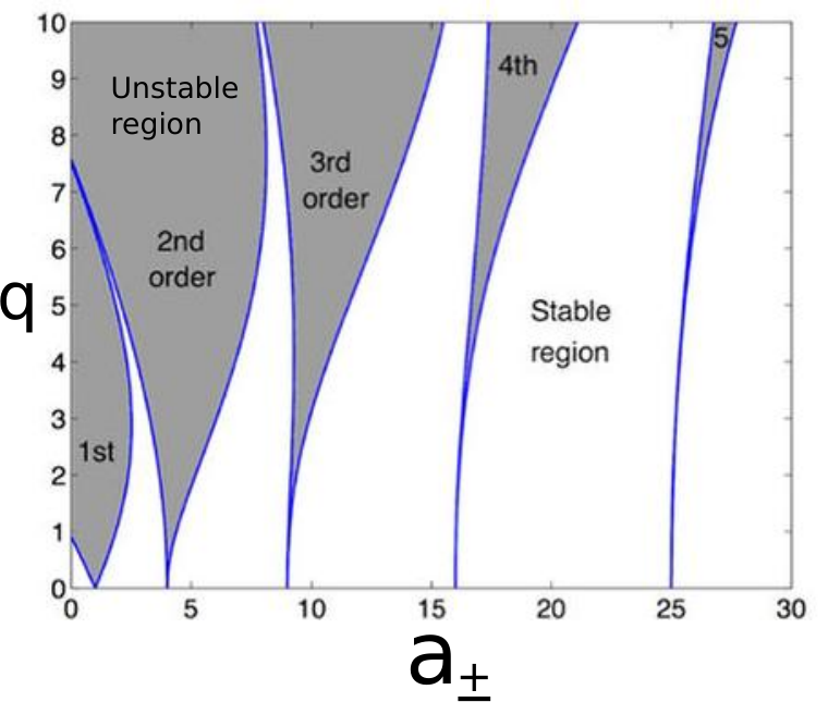
The are some important remarks concerning this equation. It describes a well known classical problem: a parametric pendulum. In such pendulum, the length is changed periodically resulting in a pattern of resonances. Fig. 2 present the allowed regions for stable solutions of the Mathieu equation, which for this problem indicates that the spectrum is made of bands and gaps. To understand the gap opening, suppose that $\tilde{k}_{\perp}=0$. As seen in Fig. 2, for $q\ll 1$ gaps are open whenever $a_{\pm}=\tilde{k}_{||}^{2}\approx n^{2}\$ with $n=1,2,3,...$ resulting in $|\bm{k}|\approx nG$, which is a diffraction condition due to the ripple wave-periodicity. Translated into energy, this condition is $E\approx nv_{F}\hbar G$, which is the energy of an electron with momentum $G$. In graphene, $\hbar v_{F}\approx 0.65775$ eV.nm, and $E\approx(4.13/\lambda)$ eV.nm if $\lambda$ is given in nanometers naumis-review. For example, $E\approx 0.0413$ eV for a ripple with $\lambda=100$ nm. As $h_{0}$ grows, $E$ decreases from this value. For $q=1$, a gap opens at the Dirac point. On the other hand, if $|\bm{\tilde{k}}|\approx\tilde{k}_{\perp}\gg 1$, then $a_{\pm}\approx q$ and the gaps become much wider, meaning that in general, the propagation is preferentially in a direction parallel to the ripple. For a fixed value of $a_{\pm}$ and $q$, the general solution is a linear combination of the Mathieu cosine $C(a_{\pm},q,\zeta)$ and Mathieu sine $S(a_{\pm},q,\zeta)$ functions. In this particular case, the solution must reduce to the free-particle wavefunction for $\tilde{A_{0}}=0$. By taking into account that $C(a_{\pm},0,\zeta)=\cos(\sqrt{a_{\pm}}\zeta)$ and $S(a_{\pm},0,\zeta)=\sin(\sqrt{a_{\pm}}\zeta)$, the solution can be written as,

$$\Gamma(\zeta_{\pm})=\left[C(a_{\pm},q,\zeta_{\pm})+iS(a_{\pm},q,\zeta_{\pm})\right]\left({\begin{array}[]{cc}1\\ s\exp(i\alpha)\\ \end{array}}\right).$$

(25)

where $s=\pm 1$, where the minus is used for the conduction and valence bands respectively. The second observation is that solutions on each valley are out of phase by a factor $2\phi_{0}$. This is an suggests a kind of quantum pump that deserves further investigation.

Let us now analyze the presence of both pseudo scalar and pseudo vectorial fields. The expression for $F(\phi)$ is in general too complicated to extract the physical behavior behind it. Instead consider first the limit $\tilde{|\bm{k}|}>>\tilde{g}$ and $\tilde{|\bm{k}|}>>\tilde{A}_{0}$. Under such assumption $F(\phi)$ is given by,

$$F(\phi)\approx\frac{C^{\prime}(\phi)}{C(\phi)}D(\phi)+C^{2}(\phi)-D^{\prime}(\phi)-D^{2}(\phi)-\frac{C^{\prime\prime}(\phi)}{2C(\phi)},$$

(26)

from where it follows that,

$$F(\phi)\approx a_{\pm}+L(\tilde{k})cos(2\phi)+M(\tilde{k})sin(2\phi),$$

(27)

with,

$$a_{\pm}=\tilde{k}_{||}^{2}+\eta\tilde{k}_{\perp}\tilde{A_{0}}\sin(3\gamma)-\tilde{g}|k|,$$

(28)

$$L(\tilde{k})=-\eta\tilde{k}_{\perp}\tilde{A_{0}}\sin(3\gamma)+\tilde{g}\left(|\tilde{\bm{k}}|-\frac{1}{|\tilde{k}|}\right),$$

(29)

$$M(\tilde{k})=-\tilde{A_{0}}\sin(3\gamma)+\eta\tilde{g}\sin(\gamma-\alpha),$$

(30)

By setting,

$$L(\tilde{k})\cos(2\phi)+M(\tilde{k})\sin(2\phi)=-2q\cos(\phi+\phi_{0}),$$

(31)

where $q$ and $\phi_{0}$ are given by,

$$q=\frac{\sqrt{L^{2}(\tilde{k})+M^{2}(\tilde{k})}}{2},$$

(32)

and

$$\tan(\phi_{0})=-\frac{M(\tilde{k})}{L(\tilde{k})}.$$

(33)

Defining a new variable $\zeta=\phi+\phi_{0}$ which takes into account the phase shift, again we obtain a Matthieu equation for $Z(\zeta)$,

$$\frac{d^{2}Z(\zeta)}{d\zeta^{2}2}+(a_{\pm}-2q\cos(2\zeta))Z(\zeta)=0.$$

(34)

Notice that for $\tilde{g}=0$, we recover exactly the case without the scalar field, while for $\tilde{g}\neq 0$, $a_{\pm}$ and $q$ are modified to include an energy correction due to the pseudoscalar field. Once the solution for $Z(\phi)$ is found by using the Matthieu functions, we obtain that,

$$\Gamma_{A}(\phi)\approx\left(1+\frac{\tilde{g}}{\tilde{k}}\sin^{2}(\phi)\right)\frac{Z(\phi)}{\tilde{k}}.$$

(35)

When $|\tilde{\bm{k}}|\leq\tilde{g}$, the previous approximations brake down. Thus a different approach is needed. For simplicity, consider the case $D(\phi)=0$. Instead of using Eq. (18), it is easier to start from Eqns. (14) and (15),

$$\Gamma_{A}^{\prime\prime}(\phi)+\frac{1}{C(\phi)}\frac{dC(\phi)}{\phi}\Gamma_{A}^{\prime}(\phi)+C(\phi))^{2}\Gamma_{A}(\phi)=0,$$

(36)

resulting in,

$$\Gamma_{A}^{\prime\prime}(\phi)+\frac{q\sin(2\phi)}{\epsilon+q\cos(2\phi)}\Gamma_{A}^{\prime}(\phi)+(\epsilon+q\cos(2\phi))^{2}\Gamma_{A}(\phi)=0,$$

(37)

with $\epsilon=\tilde{k}-\tilde{g}/2$ and $q=\tilde{g}/2$. By making the substitution $\Gamma_{A}(\phi)=u(q\sin(2\phi)+2\epsilon\phi)$, it follows that $u$ satisfies the harmonic oscillator equation, from where the solution is given by,

$$\begin{split}\Gamma_{A}(\phi)&=C_{1}\cos\left[\frac{\tilde{g}}{4}\sin(2\phi)+(\tilde{k}-\tilde{g}/4)2\phi\right]\\ &+C_{2}\sin\left[\frac{\tilde{g}}{4}\sin(2\phi)+(\tilde{k}-\tilde{g}/4)2\phi\right],\end{split}$$

(38)

where $C_{1}$ and $C_{2}$ are constants determined from the initial conditions.

Figure 3 shows a comparison between the analytical solution Eq. (38) and a numerical solution of Eqns. (14) and (15), obtained using a Runge-Kutta algorithm, showing a perfect match. Figure 3 is the solution for $\tilde{E}=\tilde{k}=0$. In this plot $\tilde{g}=10$, corresponding to $h_{0}\approx 2$ nm and $\lambda\approx 39$ nm. This value has been chosen because it is within the limits of the physical system and the Dirac approximation. To see this, consider that $\bar{g}=(g/2)(Gh_{0})^{2}$, and since $G=2\pi/\lambda$, we obtain $\bar{g}=(2\pi^{2}g)(h_{0}/\lambda)^{2}$. Then, $\tilde{g}=(2\pi^{2}g)(h_{0}/\lambda)^{2}/[v_{F}\hbar 2\pi/\lambda]$ . The biggest estimation of $g$ is $20$ eV, resulting in $\bar{g}\approx 395(h_{0}/\lambda)^{2}\text{eV}$. Finally, $\tilde{g}\approx 95(h_{0}^{2}/\lambda)\text{nm}^{-1}$. Assuming $h_{0}\approx 1\ nm$, and the minimal $\lambda\approx 1\ nm$, we have $\tilde{g}\approx 95$. From there, $\tilde{g}$ goes to zero as $\lambda\rightarrow\infty$ and $h_{0}\rightarrow 0$. However, the Dirac approximation imposes $h_{0}/\lambda<0.053$, resulting in the limit $\tilde{g}<25$ to our approach.

In both solutions, we observe regions of oscillations with a frequency determined by $\tilde{g}$ and $\tilde{k}$. Therein, the electrons are acelerated, while for certain phases, the solutions present a maximum with a wider width. It is important to remark that our solution implies the generation of high-harmonics in response to the field. To show this, assume that $C_{1}=1$ and $C_{2}=0$ in Eq. (38). Defining $\tilde{\omega}=2(\tilde{k}-\tilde{g}/4)$, using a trigonometric identity and by expanding the composition of trigonometric functions in terms of the Bessel functions $J_{p}(\tilde{g}/4)$ we obtain,

$$\begin{split}\Gamma_{A}(\phi)&=\left(J_{0}(\tilde{g}/4)+\sum_{p=1}J_{2p}(\tilde{g}/4)cos(4p\phi)\right)\cos[\tilde{\omega}\phi]\\ &-\left(\sum_{p=0}J_{2p+1}(\tilde{g}/4)cos((2p+1)2\phi)\right)\sin[\tilde{\omega}\phi].\end{split}$$

(39)

Thus, the electron dynamic response contains a rich structure of harmonics. Observe also that the zeros of the Bessel functions allows to tune the pseudoscalar field in such a way that certain harmonics can be eliminated.

We end up by showing in Fig. 4 a numerical solution of the case in which both pseudoscalar and pseudovectorial fields are present. The mains differences are the modification of the oscillating frequency and that the regions of nearly constant amplitude present more structure, instead of a maximum.

In conclusion, we have solved the problem of electrons in graphene under a propagating ripple. This was done by solving a Dirac equation which includes the corresponding propagating pseudoscalar and pseudovectorial fields. In the presence of a ripple with only a pseudovectorial field, the equation can be transformed into an ordinary second-order partial equation, i.e., into the Matthieu equation. Such system presents a spectrum made from gaps and bands. Gaps are basically determined from electron diffraction by ripple waves. Also, electron propagation happens mainly in the ripple-propagation-direction. For the presence of both a pseudovectorial and pseudoscalar field, we also found a Matthieu equations with a spectrum of bands and gaps but with different parameters. However, when the energy of the electron is less than the energy associated to the pseudoscalar field, a different kind of equation is obtained. For the pure pseudoscalar field, no gaps are observed. In all cases, the solutions contain high-harmonics with respect to the fundamental frequency of the driving field.

R.C.B acknowledges useful discussions with M. Asmar and I. Vekhter. This work was supported by project UNAM-DGAPA-PAPIIT-IN102717 and Movilidad Académica 2017 (UABC).

References

- [1] Jin-Wu Jiang, Bing-Shen Wang, Jian-Sheng Wang, and Harold S Park. A review on the flexural mode of graphene: lattice dynamics, thermal conduction, thermal expansion, elasticity and nanomechanical resonance. Journal of Physics: Condensed Matter, 27(8):083001, 2015.
- [2] Jin-Wu Jiang, Hui Tang, Bing-Shen Wang, and Zhao-Bin Su. Chiral symmetry analysis and rigid rotational invariance for the lattice dynamics of single-wall carbon nanotubes. Phys. Rev. B, 73:235434, Jun 2006.
- [3] AH Castro Neto, F Guinea, Nuno MR Peres, Kostya S Novoselov, and Andre K Geim. The electronic properties of graphene. Reviews of modern physics, 81(1):109, 2009.
- [4] José González, Francisco Guinea, and M. Angeles H. Vozmediano. Continuum approximation to fullerene molecules. Phys. Rev. Lett., 69:172–175, Jul 1992.
- [5] C. L. Kane and E. J. Mele. Size, shape, and low energy electronic structure of carbon nanotubes. Phys. Rev. Lett., 78:1932–1935, Mar 1997.
- [6] María AH Vozmediano, MI Katsnelson, and Francisco Guinea. Gauge fields in graphene. Physics Reports, 496(4):109–148, 2010.
- [7] Gerardo G Naumis, Salvador Barraza-Lopez, Maurice Oliva-Leyva, and Humberto Terrones. Electronic and optical properties of strained graphene and other strained 2d materials: a review. Reports on Progress in Physics, 80(9):096501, 2017.
- [8] Hidekatsu Suzuura and Tsuneya Ando. Phonons and electron-phonon scattering in carbon nanotubes. Physical review B, 65(23):235412, 2002.
- [9] B. Amorim, A. Cortijo, F. de Juan, A.G. Grushin, F. Guinea, A. Gutiérrez-Rubio, H. Ochoa, V. Parente, R. Roldán, P. San-Jose, J. Schiefele, M. Sturla, and M.A.H. Vozmediano. Novel effects of strains in graphene and other two dimensional materials. Physics Reports, 617:1 – 54, 2016. Novel effects of strains in graphene and other two dimensional materials.
- [10] Cheol-Hwan Park, Nicola Bonini, Thibault Sohier, Georgy Samsonidze, Boris Kozinsky, Matteo Calandra, Francesco Mauri, and Nicola Marzari. Electron–phonon interactions and the intrinsic electrical resistivity of graphene. Nano Letters, 14(3):1113–1119, 2014. PMID: 24524418.
- [11] Thibault Sohier, Matteo Calandra, Cheol-Hwan Park, Nicola Bonini, Nicola Marzari, and Francesco Mauri. Phonon-limited resistivity of graphene by first-principles calculations: Electron-phonon interactions, strain-induced gauge field, and boltzmann equation. Phys. Rev. B, 90:125414, Sep 2014.
- [12] James V. Sloan, Alejandro A. Pacheco Sanjuan, Zhengfei Wang, Cedric Horvath, and Salvador Barraza-Lopez. Strain gauge fields for rippled graphene membranes under central mechanical load: An approach beyond first-order continuum elasticity. Phys. Rev. B, 87:155436, Apr 2013.
- [13] N Levy, SA Burke, KL Meaker, M Panlasigui, A Zettl, F Guinea, AH Castro Neto, and MF Crommie. Strain-induced pseudo–magnetic fields greater than 300 tesla in graphene nanobubbles. Science, 329(5991):544–547, 2010.
- [14] Francisco Guinea, MI Katsnelson, and AK Geim. Energy gaps and a zero-field quantum hall effect in graphene by strain engineering. Nature Physics, 6(1):30, 2010.
- [15] Ken-ichi Sasaki and Riichiro Saito. Pseudospin and deformation-induced gauge field in graphene. Progress of Theoretical Physics Supplement, 176:253–278, 2008.
- [16] Alexander Georgi, Peter Nemes-Incze, Ramon Carrillo-Bastos, Daiara Faria, Silvia Viola Kusminskiy, Dawei Zhai, Martin Schneider, Dinesh Subramaniam, Torge Mashoff, Nils M Freitag, et al. Tuning the pseudospin polarization of graphene by a pseudomagnetic field. Nano letters, 17(4):2240–2245, 2017.
- [17] ML Ackerman, P Kumar, M Neek-Amal, PM Thibado, FM Peeters, and Surendra Singh. Anomalous dynamical behavior of freestanding graphene membranes. Physical review letters, 117(12):126801, 2016.
- [18] YZ He, Hui Li, PC Si, YF Li, HQ Yu, XQ Zhang, F Ding, Kim Meow Liew, and XF Liu. Dynamic ripples in single layer graphene. Applied physics letters, 98(6):063101, 2011.
- [19] EA Korznikova and SV Dmitriev. Moving wrinklon in graphene nanoribbons. Journal of Physics D: Applied Physics, 47(34):345307, 2014.
- [20] Tony Low, Yongjin Jiang, Mikhail Katsnelson, and Francisco Guinea. Electron pumping in graphene mechanical resonators. Nano letters, 12(2):850–854, 2012.
- [21] Abolhassan Vaezi, Nima Abedpour, Reza Asgari, Alberto Cortijo, and María AH Vozmediano. Topological electric current from time-dependent elastic deformations in graphene. Physical Review B, 88(12):125406, 2013.
- [22] Yongjin Jiang, Tony Low, Kai Chang, Mikhail I Katsnelson, and Francisco Guinea. Generation of pure bulk valley current in graphene. Physical review letters, 110(4):046601, 2013.
- [23] Kai Zhang, Erhu Zhang, Huawei Chen, and Shengli Zhang. Odd-parity currents induced by dynamic deformations in graphene-like systems. Journal of Physics: Condensed Matter, 28(45):455301, 2016.
- [24] Pedro Roman-Taboada and Gerardo G Naumis. Topological phase-diagram of time-periodically rippled zigzag graphene nanoribbons. Journal of Physics Communications, 1(5):055023, 2017.
- [25] Pedro Roman-Taboada and Gerardo G Naumis. Topological edge states on time-periodically strained armchair graphene nanoribbons. Physical Review B, 96(15):155435, 2017.
- [26] Pedro Roman-Taboada and Gerardo G Naumis. Topological flat bands in time-periodically driven uniaxial strained graphene nanoribbons. Physical Review B, 95(11):115440, 2017.
- [27] Thomas Iadecola, David Campbell, Claudio Chamon, Chang-Yu Hou, Roman Jackiw, So-Young Pi, and Silvia Viola Kusminskiy. Materials design from nonequilibrium steady states: driven graphene as a tunable semiconductor with topological properties. Physical review letters, 110(17):176603, 2013.
- [28] Thomas Iadecola, Titus Neupert, and Claudio Chamon. Topological gaps without masses in driven graphene-like systems. Physical Review B, 89(11):115425, 2014.
- [29] Hannes Hübener, Umberto De Giovannini, and Angel Rubio. Phonon driven floquet matter. Nano Letters, 0(0):null, 0. PMID: 29361223.
- [30] Mircea Trif, Pramey Upadhyaya, and Yaroslav Tserkovnyak. Theory of electromechanical coupling in dynamical graphene. Physical Review B, 88(24):245423, 2013.
- [31] Ken-ichi Sasaki, Hideki Gotoh, and Yasuhiro Tokura. Valley-antisymmetric potential in graphene under dynamical deformation. Physical Review B, 90(20):205402, 2014.
- [32] M Oliva-Leyva and Gerardo G Naumis. Sound waves induce volkov-like states, band structure and collimation effect in graphene. Journal of Physics: Condensed Matter, 28(2):025301, 2015.
- [33] FJ López-Rodríguez and GG Naumis. Analytic solution for electrons and holes in graphene under electromagnetic waves: gap appearance and nonlinear effects. Physical Review B, 78(20):201406, 2008.
- [34] Richard Kerner, Gerardo G Naumis, and Wilfrido A Gómez-Arias. Bending and flexural phonon scattering: Generalized dirac equation for an electron moving in curved graphene. Physica B: Condensed Matter, 407(12):2002–2008, 2012.
- [35] J Scott Bunch, Arend M Van Der Zande, Scott S Verbridge, Ian W Frank, David M Tanenbaum, Jeevak M Parpia, Harold G Craighead, and Paul L McEuen. Electromechanical resonators from graphene sheets. Science, 315(5811):490–493, 2007.
- [36] Péter Nemes-Incze, Gergő Kukucska, János Koltai, Jenő Kürti, Chanyong Hwang, Levente Tapasztó, and László P Biró. Preparing local strain patterns in graphene by atomic force microscope based indentation. Scientific Reports, 7(1):3035, 2017.
- [37] Nikolai N. Klimov, Suyong Jung, Shuze Zhu, Teng Li, C. Alan Wright, Santiago D. Solares, David B. Newell, Nikolai B. Zhitenev, and Joseph A. Stroscio. Electromechanical properties of graphene drumheads. Science, 336(6088):1557–1561, 2012.
- [38] U. Monteverde, J. Pal, M.A. Migliorato, M. Missous, U. Bangert, R. Zan, R. Kashtiban, and D. Powell. Under pressure: Control of strain, phonons and bandgap opening in rippled graphene. Carbon, 91:266 – 274, 2015.
- [39] Yong Wu, Dawei Zhai, Cheng Pan, Bin Cheng, Takashi Taniguchi, Kenji Watanabe, Nancy Sandler, and Marc Bockrath. Quantum wires and waveguides formed in graphene by strain. Nano letters, 18(1):64–69, 2017.
- [40] Ken-ichi Sasaki and Riichiro Saito. Pseudospin and deformation-induced gauge field in graphene. Progress of Theoretical Physics Supplement, 176:253–278, 2008.
- [41] Lev Davidovich Landau and Eugin M Lifshitz. Course of Theoretical Physics Vol 7: Theory and Elasticity. Pergamon Press, 1959.
- [42] Ke-Ke Bai, Yu Zhou, Hong Zheng, Lan Meng, Hailin Peng, Zhongfan Liu, Jia-Cai Nie, and Lin He. Creating one-dimensional nanoscale periodic ripples in a continuous mosaic graphene monolayer. Phys. Rev. Lett., 113:086102, Aug 2014.
- [43] Lev Davidovich Landau and Eugin M Lifshitz. Physique Téorique Vol 4: Electrodynamique quantique. Editions Mir, Moscow, 1989.
- [44] Lev Davidovich Landau and Eugin M Lifshitz. Course of Theoretical Physics Vol 7: Quantum Electrodynamics. Pergamon Press, 1959.