Magnetic field driven enhancement of the weak decay width of charged pions
Abstract
We study the effect of a uniform magnetic field on the decays , where , carrying out a general analysis that includes four decay constants. Taking the values of these constants from a chiral effective Nambu-Jona–Lasinio (NJL) model, it is seen that the total decay rate gets strongly increased with respect to the case, with an enhancement factor ranging from for up to for . The ratio between electronic and muonic decays gets also enhanced, reaching a value of about for . In addition, we find that for large the angular distribution of outgoing antineutrinos shows a significant suppression in the direction of the magnetic field.
I Introduction
The effect of intense magnetic fields on the properties of strongly interacting matter has gained significant interest in recent years Kharzeev:2012ph; Andersen:2014xxa; Miransky:2015ava. This is mostly motivated by the realization that strong magnetic fields might play an important role in the study of the early Universe Grasso:2000wj, in the analysis of high energy non-central heavy ion collisions Kharzeev; Skokov; Voronyuk, and in the description of compact stellar objects like the magnetars Duncan; Kouveliotou. It is well known that magnetic fields also induce interesting phenomena such as the enhancement of the QCD vacuum (the so-called “magnetic catalysis”) Gusynin:1994re and the decrease of critical temperatures for chiral restoration and deconfinement QCD transitions Bali:2011qj; Bali:2012zg. In this work we concentrate on the effect of a magnetic field on the weak pion-to-lepton decays , where . In fact, the study of weak decays of hadrons in the presence of strong electromagnetic fields has a rather long history (see e.g. refs. Nikishov:1964zza; Nikishov:1964zz; Matese:1969zz; FassioCanuto:1970wk). In most of the existing calculations of these decay rates, however, the effect of the external field on the internal structure of the participating particles has not been taken into account. In the case of charged pions, only recently such an effect has been analyzed in the context of chiral perturbation theory Andersen:2012zc and effective chiral models Simonov:2015xta; Liu:2018zag; Coppola:2018vkw, as well as through lattice QCD (LQCD) calculations Bali:2018sey. In ref. Bali:2018sey it is noted that the existence of the background field opens the possibility of a nonzero pion-to-vacuum transition via the vector piece of the hadronic current, implying the existence of a further form factor in addition to the pion decay constant (which arises from the axial vector piece). Taking into account this new decay constant and using some approximations for the dynamics of the participating particles, the authors of ref. Bali:2018sey obtain an expression for the decay width in the presence of the external field. In particular, it is claimed that for GeV2, being the proton charge, the decay rate of charged pions into muons could be enhanced by a factor of about 50 with respect to its value at . Recently, a more complete analysis of the situation has been presented in ref. Coppola:2018ygv, where the most general form of the relevant hadronic matrix elements in the presence of an external uniform magnetic field was determined. It was found that in general the vector and axial vector pion-to-vacuum transitions (for the case of charged pions) can be parametrized through one and three hadronic form factors, respectively. Taking into account all four decay constants, in ref. Coppola:2018ygv an expression for the decay width that fully takes into account the effect of the magnetic field on both pion and lepton wave functions was obtained using the Landau gauge. The same expression was found in ref. Coppola:2019wvh using the symmetric gauge, explicitly showing the gauge independence of the result.
The main purpose of this article is to show that, once the above-mentioned improvements are incorporated, the decay rate in the presence of the magnetic field turns out to be strongly enhanced with respect to its value for . Taking values for the decay constants from an effective Nambu-Jona-Lasinio (NJL) model, this enhancement is found to range from for GeV2 up to for GeV2. Interestingly, it is found that the ratio between partial decay rates into electrons and muons gets also significantly increased, reaching a value of about 0.5 for GeV2. In addition, it is observed that already for GeV2 the angular distribution of the outgoing antineutrinos is expected to be highly anisotropic, showing a significant suppression in the direction of the magnetic field.
The paper is organized as follows. In sec. II we present a general theoretical analysis of the decay width in the presence of the external field. This includes a comparison with the case and a discussion on the lack of the helicity suppression mechanism. In sec. III, numerical estimations are given in the framework of the NJL model. Finally, in sec. IV we summarize our research and provide some conclusions. We also include two appendices. In appendix A we present a brief discussion on the relation between gauge invariance and axial rotations, while in appendix B we give some expressions for pion and lepton wavefunctions in the presence of the magnetic field.
II decay
II.1 Absence of helicity suppression for nonzero external magnetic field
As well known, if there is no external magnetic field the decay width in the pion rest frame is given by
| (1) |
where is the Fermi effective coupling, is the Cabibbo angle, and the value of the decay constant MeV can be obtained from the empirical mean lifetime s Tanabashi:2018oca. Owing to the factor, the total width is strongly dominated by the muonic decay, for which the branching ratio reaches about 99.99%. The reason for this behavior can be easily understood in terms of “helicity suppression”. In the pion rest frame, the outgoing charged lepton and antineutrino have opposite momenta, therefore the final state has zero orbital angular momentum, and angular momentum conservation requires both outgoing particles to have opposite spins. Taking the direction of the momenta as the angular momentum quantization axis, this implies that the charged lepton and the antineutrino should have the same helicity. On the other hand, the electroweak current couples the only to right-handed antineutrinos and left-handed charged leptons. Then, if we assume that neutrinos are massless, the helicity of the antineutrino will be . In the limit the helicity of the left-handed charged lepton will be , i.e. opposite to that of the antineutrino. Since this is in contradiction with the result above, the decay turns out to be forbidden in that limit.
In the presence of an external uniform magnetic , the above situation becomes dramatically modified. For definiteness, let us take the magnetic field to lie along the axis, , with . As in the case, we assume the charged pion to be in its lowest possible energy state. The latter corresponds to the lowest Landau level (LLL) , and the pion component of the momentum . It is worth stressing that, even in this lowest energy state, the decaying pion cannot be at rest, due to the existence of a nonvanishing zero-point motion. In fact, the three spacial components of pion momentum are not a good set of quantum numbers to describe the initial state in this case. Moreover, the outcomes obtained for from angular momentum conservation do not apply for nonzero . The analysis of the decay in terms of angular momenta of the initial and final states is not straightforward, since for nonzero canonical angular momenta of charged particles turn out to be gauge dependent quantities, and total mechanical angular momentum is in general not conserved Li; Greenshields; Wakamatsu:2017isl; Coppola:2019wvh. A brief discussion on how this can be reconciled with the rotational invariance of the system is included in appendix A.
To have a better understanding of the situation, it is interesting to consider the case in which the magnitude of the magnetic field is large enough so that the outgoing charged lepton can only be in the LLL, (the validity of this assumption will be discussed below). Considering the explicit form of the corresponding spinors Coppola:2018ygv; Coppola:2019wvh, it is not hard to show (see appendix B) that in the limit one has
| (2) |
where is the mechanical linear momentum operator (a gauge invariant quantity) and is the component of the momentum of the charged lepton. As expected, the chirality of the LLL lepton state coincides with its helicity in the massless limit. Interestingly, in eq. (2) only the parallel piece of the helicity operator contributes. This can be understood by noting that for the LLL only one polarization state, namely that associated to , is allowed (see appendix B). Being and polarization-changing operators, the action of the sum on the state has to vanish in order to ensure that the latter is an helicity eigenstate, as it should be in the limit. Let us consider now the outgoing antineutrino, taking it to be in a state of momentum . Since it has to be right-handed, the helicity operator satisfies
| (3) |
In this case, however, the transverse piece of the helicity operator provides in general a nonvanishing contribution. On one hand, there is no restriction for antineutrino helicity eigenstates to be in general a combination of the two available possible polarization states, Coppola:2018ygv; Coppola:2019wvh. On the other hand, the antineutrino transverse momentum is in general nonvanishing, since, due to zero-point motion, the wavefunctions of charged particles in the LLL involve a superposition of various transverse momenta. Therefore, eq. (3) does not determine the sign of , and nothing forces the outgoing particles to have the same helicity, in contrast with the case. Thus, no helicity suppression mechanism is present for nonzero , and, consequently, the decay amplitude does not necessarily vanish in the limit.
To quantitatively see how important the “non-helicity suppression” effect is, one has to analyze in detail the decay width in the presence of the magnetic field. A model independent expression for the width has been obtained in refs. Coppola:2018ygv; Coppola:2019wvh, taking the decaying pion to be in the LLL, with . The main steps leading to this expression are summarized in the following subsections.
II.2 Particle states and gauge choice
The actual calculation of the partial widths for nonzero external magnetic field requires to choose a specific gauge. We note, however, that the widths are expected to be gauge independent, as explicitly shown in refs. Coppola:2018ygv and Coppola:2019wvh, where the same result has been obtained considering the Landau and symmetric gauges, respectively. Here we will retrieve some of the steps followed for the case of the symmetric gauge, in which one has axial symmetry and the participating particles can be expressed in terms of states of well defined angular momentum projection in the direction of the external field.
For our calculations we adopt the following conventions. For a space-time coordinate four-vector we use the notation , taking the Minkowski metric . We assume the presence of a uniform static magnetic field , and orientate the spatial axes in such a way that , with . Owing to axial symmetry, it is convenient to use for standard cylindrical coordinates , and . The vector potential will be then given by , with .
As already mentioned, in the presence of an external magnetic field the three spacial components of momentum are not a good set of quantum numbers for charged particles. In fact, in the plane perpendicular to , charged particle states are quantized in Landau levels. For the symmetric gauge, given our axis choice, one can define a complete basis of states of well defined energy taking as quantum numbers the component of the momentum, the Landau level and the component of the canonical total angular momentum . For the antineutrino, having zero electric charge, we take , and , where is the antineutrino linear momentum. The notation used for the quantum numbers of the , and is summarized in table 1. Here , , , and are non-negative integers, is an integer, and . To this set of quantum numbers one has to add the polarization () of the charged lepton (we assume the antineutrino to be purely righthanded). Notice that, although it is not indicated explicitly, the pion mass is a function of the magnetic field . The explicit form of the , and wavefunctions and spinors in the symmetric gauge is quoted in appendix B.
| Pion | Lepton | Antineutrino | |
|---|---|---|---|
| Parallel momentum | |||
| Landau level | – | ||
| Energy | |||
| Shorthand notation |
II.3 Decay amplitude
According to the notation introduced in the previous subsection, the transition matrix element for the decay is given by . As usual, the amplitude can be written in terms of leptonic and hadronic parts. Taking into account the expressions for the involved fields quoted in appendix B (for more details, see also ref. Coppola:2019wvh) one gets
| (4) |
where stands for the matrix element of the hadronic current,
| (5) |
The matrix element in eq. (5) involves strong interactions in a low energy regime and cannot be treated perturbatively. Instead, it can be parameterized in terms of decay form factors taking into account the Lorentz structure and the symmetries of the theory. As it is well known, in the absence of external fields the amplitude can be written in terms of a single form factor, namely, the pion decay constant . In that case, owing to parity symmetry, only the axial-vector piece can be nonzero. However, when a static external electromagnetic field is present, several independent tensor structures are allowed and four independent form factors can be defined. Three of them correspond to the axial-vector and one to the vector piece of the hadronic current. Following ref. Coppola:2018ygv, the hadronic matrix element in eq. (5) can be parameterized as
| (6) | |||||
where is the electromagnetic field tensor, and . It can be seen that the discrete symmetries of the interaction Lagrangian restrict all four form factors to be real Coppola:2018ygv. In the symmetric gauge, taking into account the expression for quoted in appendix B, and defining “parallel” and “perpendicular” pieces and , one gets
| (7) | ||||||
| (8) | ||||||
where we have used the notation .
Using these expressions together with the explicit form of the functions , and , one can perform the spatial integral in eq. (4) to get
| (9) | |||||
The explicit form of the function , as well as details of the calculation, can be found in ref. Coppola:2019wvh. As expected from the symmetries of the Lagrangian, eq. (9) shows the conservation of the total energy and the component of the momentum. Moreover, from table 1 it is seen that the Kronecker delta in eq. (9) implies , i.e., the component of the total canonical angular momentum is also conserved. This is not a general property but a particular feature of the calculation in the symmetric gauge, in which the Lagrangian is invariant under axial rotations. We recall that, in the presence of the external magnetic field, the canonical angular momentum is not a gauge invariant quantity and does not represent a physical observable.
II.4 Partial decay width
The width for the decay is given by
| (10) |
where and are the time interval and length on the -axis in which the interaction is active. At the end of the calculation, the limit should be taken. From the result in eq. (9) we get
| (11) |
where
| (12) |
Now, as it is usually done, we concentrate on the situation in which the decaying pion is in the lowest energy state. This corresponds to and , hence . Here we will quote the final expression obtained for the decay width. Details of the calculation can be found in ref. Coppola:2019wvh. The result can be expressed in terms of three form factor combinations , and , given by
| (13) |
One has Coppola:2019wvh
| (14) |
where the function is given by
| (15) | |||||
and we have used the definitions , and
| (16) |
The integration variable chosen here is . The sum over and the integrals over and can be calculated with the help of the deltas, while the sum over can be performed analytically.
As expected, the decay width does not depend on the quantum number . The latter determines the canonical angular momentum of the decaying pion, which, as stated, is a gauge dependent quantity. Though the expression of the decay amplitude will vary in general for different gauge choices, it is clear that the result for the decay width in eq. (14) has to be gauge independent. Indeed, the same result for has been found in ref. Coppola:2018ygv using the Landau gauge.
As discussed in the previous subsection, the decay constants in eq. (13) parameterize the most general form of the pion-to-vacuum vector and axial vector hadronic matrix elements. Their theoretical determination would require either to use LQCD simulations or to rely on some hadronic effective model. Before addressing possible estimates for these quantities, let us analyze how “non-helicity suppression” is realized in eq. (14). Once again we concentrate in the case of a large external magnetic field. Since the pion is built of charged quarks, the pion mass will depend in general on the magnetic field. Now, if the mass growth is relatively mild, for large magnetic fields one should get . In fact, this is what one obtains from lattice QCD calculations Bali:2018sey as well as from effective approaches like the Nambu-Jona–Lasinio model Coppola:2018vkw, for values of say GeV2. According to the above expressions, this implies , hence the outgoing muon or electron (let us assume that the energy is below the production threshold) is expected to lie in its LLL (), where only one polarization state is allowed. A further simplification can be obtained when the squared lepton mass can be neglected in comparison with (or, equivalently, in comparison with , which is expected to grow approximately as ). For , one can take . Then, and the integral over extends up to . In this limit the decay width is given by
| (17) |
As anticipated, there is no helicity suppression, and the width does not vanish in the limit. In fact, it turns out to grow with the magnetic field as , with some suppression due to the factor in square brackets. Clearly, the physical relevance of eq. (17) depends on whether the term proportional to the form factor combination on the right hand side is the dominant one in the full expression for the decay width. As can be seen from eq. (15), the terms involving the form factor —which, in general, would compete with the form factors in eq. (17)— become negligible in the limit . While in the case of the decay to this should be a good approximation already for GeV2, for decays into muons (and taus) the situation is less clear, and corrections arising from a nonzero lepton mass should be taken into account.
III Numerical results within the NJL model
In order to provide actual estimates for the magnetic field dependence of the decay width we need some input values for the decay constants. Although some results have been provided by existing LQCD simulations Bali:2018sey, present lattice analyses involve relatively large error bars and, moreover, only include the calculation of the form factors and . Therefore, we will consider here the values calculated in ref. Coppola:2019uyr for all four form factors in the framework of the NJL model. In fact, beyond the first lattice data points, results from ref. Bali:2018sey show an overall increase in with the magnetic field, in qualitative agreement with the values obtained from NJL model calculations Coppola:2019uyr. For , NJL predictions are compatible within errors with lattice data, which have been obtained for up to 0.3 GeV2 Bali:2018sey; Coppola:2019uyr.
III.1 and decay widths
Our results for the decay widths are shown in figure 1. They correspond to the parameter set denoted by “Set I” in ref. Coppola:2019uyr. In the upper left panel we quote the partial decay widths to both and as functions of , in a logarithmic scale. It is seen that the partial widths become strongly enhanced when the magnetic field is increased above say 0.1 GeV. This enhancement is more pronounced for the decay to (dashed line), since for low values of helicity suppression becomes important. The bump observed in this curve for GeV2 is due to the fact that this region is dominated by the Landau level contribution, which disappears at about GeV2 leaving as the only energetically allowed electron Landau level. The dotted line in the graph corresponds to the asymptotic decay width quoted in eq. (17). In the upper right panel we quote the ratio as a function of . The absence of helicity suppression leads to a strong increase of this ratio with the magnetic field, reaching a value of about 0.5 for GeV2, while for one has . In the lower panels we show the behavior of the total decay width , normalized to its value at . For this effective model the enhancement factor is found to be about 1000 for GeV2. Left and right panels show our results in logarithmic and linear scales, respectively. To have an estimation of the relative significance of the contribution coming from the vector piece of the hadronic amplitude, in the left panel we show with a dotted line the result obtained for the total width after setting . For large the correction will be given by a global factor, as can be seen from eq. (17). In the right panel we include for comparison the results arising form LQCD calculations quoted in ref. Bali:2018sey, which cover values of up to about 0.45 GeV2. Dark and light gray regions correspond to staggered and quenched Wilson quarks, respectively. Although these LQCD results also predict a significant growth of the total width with the magnetic field, it is seen that in our case the slope of the curve gets more rapidly enhanced with . This is, in part, due to the channel contribution. It is worth to remark that our results for the ratio are different from those obtained in ref. Bali:2018sey, where helicity suppression leads to a ratio of the order of that becomes almost independent of the magnetic field. Finally, it is important to mention that the results in figure 1 do not depend significantly on the model parametrization (e.g. it is seen that the results for parameter Sets II and III of ref. Coppola:2019uyr do not differ from those in figure 1 by more than 3%).

III.2 Angular distribution of outgoing neutrinos
It is also interesting to discuss with some detail the angular distribution of the outgoing antineutrinos. While for the distribution is isotropic, this changes significantly in the presence of a large magnetic field. Denoting , the differential decay rate can be written as
| (18) |
where
| (19) |
and the function is defined as
| (20) |
The term proportional to in eq. (18) vanishes after integration over , therefore it does not contribute to the total decay width.
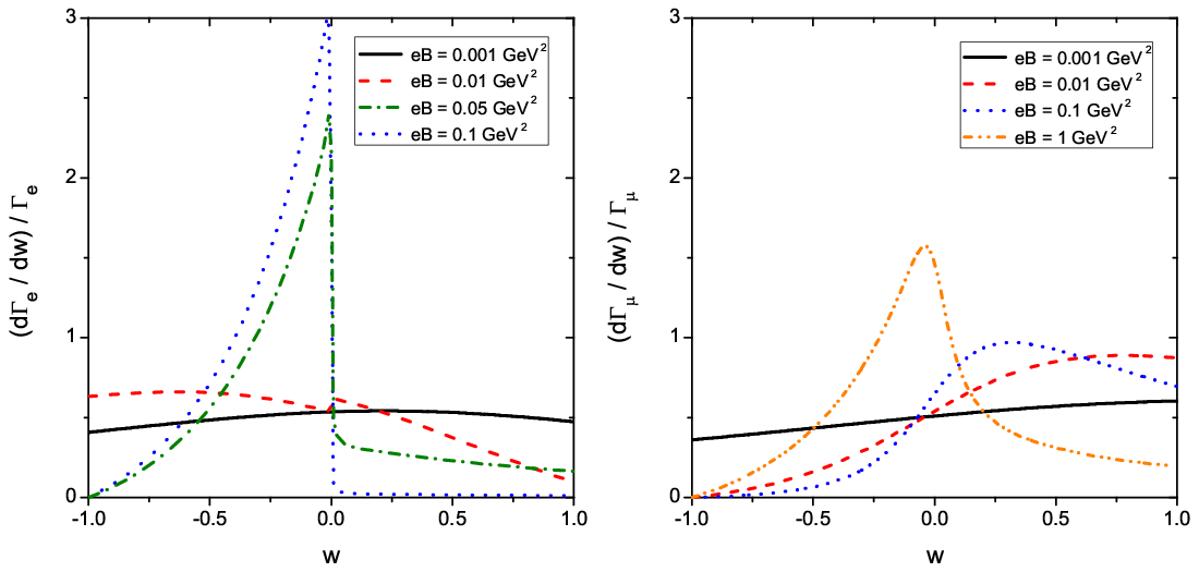
Once again, to get definite predictions for the angular distributions we rely on the values for the pion mass and decay constants obtained in ref. Coppola:2019uyr within the NJL model, taking the parameter Set I. Our numerical results for the normalized differential partial decay widths are shown in figure 2, where several representative values of are considered. Left and right panels correspond to decays into and , respectively. It is seen that the fraction of antineutrinos that come out in the half-space fluctuates when the magnetic field is increased, becoming strongly suppressed for values of much larger than the lepton mass squared. This can be qualitatively understood as follows. When , only is allowed. In addition, in the massless limit the lepton has to be left-handed, therefore from eq. (2) one gets . Conservation of the component of total momentum implies . Hence, for large , in the limit all antineutrinos should be produced with momenta in the half-space . Indeed, for and the normalized differential decay width is given by
| (21) |
where . In addition, it is worth noticing that for large values of most antineutrinos come out with low , i.e. in directions approximately perpendicular to the magnetic field.
IV Summary and conclusions
In this article we get an estimation of the effect of an external uniform magnetic field on the magnitude of the decay rate and the angular distribution of the antineutrinos in the final state. Our analysis takes into account the contribution of all four possible decay form factors. The values of these constants and that of the pion mass are taken from a NJL model for effective strong interactions, considering the in its lowest possible energy state. Our results show that the total decay rate becomes strongly increased with respect to its value at , the enhancement factor ranging from for GeV2 up to for GeV2. Moreover, owing to the presence of the new decay constants and the features of nonzero kinematics, it is found that the decay width does not vanish in the limit . As a consequence, for large values of the ratio changes dramatically with respect to the value (of about ), reaching a magnitude of at GeV2. This could be interesting e.g. regarding the expected flavor composition of neutrino fluxes coming from the cores of magnetars and other stellar objects. Finally, it is found that for large the angular distribution of outgoing antineutrinos is expected to be highly anisotropic, showing a significant suppression in the direction of the external field.
Acknowledgements.
This work has been supported in part by Consejo Nacional de Investigaciones Científicas y Técnicas and Agencia Nacional de Promoción Científica y Tecnológica (Argentina), under Grants No. PIP17-700 and No. PICT17-03-0571, respectively; by the National University of La Plata (Argentina), Project No. X824; by the MICINN (Spain), under Contract No. FPA2016-77177-C2-1-P, PID2019-105439GB-C21 and by EU Horizon 2020 Grant No. 824093 (STRONG-2020).Appendix A Axial rotations and gauge invariance
The consequences of the invariance of the physical system under rotations in the plane perpendicular to the magnetic field, as well as the relation of this invariance with the conservation of the corresponding component of the angular momentum, are delicate issues that deserve some extra comments.
Let us consider a charged pion in the presence of a uniform magnetic field, using the conventions stated in the main text of this work. Given the symmetry of the physical system, any observable is expected to be invariant under rotations about the axis. However, it is worth noticing that the Lagrangian and the action that describe the system at the quantum mechanical level are given in terms of the electromagnetic four-vector potential. Thus, they are not necessarily invariant under these rotations. For the particular case of the symmetric gauge used in this work, rotational symmetry is manifest. However, in general this will be not true for other gauges. To illustrate this point let us consider the Landau gauge (LG), in which . A spatial rotation by an angle about the axis changes into , which is given by
| (22) |
The breakdown of the invariance of the Lagrangian under this rotation is manifest. Moreover, it can be checked that in the LG neither the component of the canonical angular momentum nor that of the mechanical angular momentum commute with the Hamiltonian of the system, i.e., they are not conserved quantities. In order to reconcile this result with the expected invariance of the physical quantities under spatial rotations, we can observe that can also be written as
| (23) |
with
| (24) |
In this way, it is seen that the rotated system is connected to a gauge transformed system through a gauge transformation defined by . This shows that, in the Landau gauge, performing a spatial rotation about the axis is equivalent to performing a specific gauge transformation. Thus, in this gauge the expected invariance of physical observables under spatial rotations is guaranteed by the gauge invariance of the system.
Let us illustrate the previous statement for the case of the field. As discussed in appendix A.2 of ref. Coppola:2018ygv, in the Landau gauge the wavefunction can be written as
| (25) |
where are cylindrical parabolic functions, and we have defined and . After a rotation by an angle about the axis, one gets a rotated wavefunction given by
| (26) |
On the other hand, performing the gauge transformation defined in eqs. (23) and (24), the pion wave function in eq. (25) transforms into , given by
| (27) |
Obviously, and are different. However, they are connected in the sense that they share the same subspace of defined values of energy and momentum . This subspace is built varying the value of , which is not gauge invariant and therefore cannot be taken as a physical quantity Coppola:2018ygv.
The fact that the functions and belong to the same subspace of energy and momentum can be verified by projecting one function onto the other. One has
| (28) | |||||
which proves our statement, taking into account the (gauge independent)
relation . As a check of
the completeness of the transformed functions, it can be seen that
| (29) |
Appendix B Particle fields under a uniform magnetic field in the symmetric gauge
For convenience, we quote in this appendix the main expressions for , and fields in the presence of a magnetic field together with the eigenvalues of some relevant operators. For a more detailed description, see e.g. refs. Coppola:2019wvh and Sokolov:1986nk.
According to our conventions, the field can be written as Coppola:2019wvh
| (30) |
where , with and . The functions are solutions of the eigenvalue equation
| (31) |
where . Using cylindrical coordinates, their explicit form is given by
| (32) |
where
| (33) |
Here we have used the definitions and , while are the associated Laguerre polynomials.
The charged lepton fields in this gauge can be written as
| (34) |
where and . For , in the Weyl basis, the spinors in eq. (34) are given by
where . In the particular case of the lowest Landau level (LLL) , from these equations it is seen that , i.e., only one polarization state is allowed in each case. Using the notation , the explicit forms of the spinors are
It is interesting to consider in this context the canonical orbital angular momentum operator and the spin operator . Given the fact that the magnetic field breaks rotational invariance, only the components of these operators are relevant. These are given by and . Defining the canonical total angular momentum as , one obtains
| (61) |
Thus, as expected from axial symmetry, it is seen that for the charged leptons in the symmetric gauge one can find energy eigenstates that are also eigenstates of . It is worth noticing that only the total canonical angular momentum is well-defined, i.e., energy eigenstates are not in general eigenstates of and separately.
Let us consider now the limit in which the charged lepton mass vanishes. This is interesting when the magnetic field is relatively strong, say . In the limit the chirality operator becomes equivalent to the helicity operator and commutes with the Hamiltonian. Consequently, one can obtain energy eigenstates of well defined chirality/helicity as linear combinations of the two polarization states. In the particular case of the LLL, since only one polarization state is available, it has to be a helicity eigenstate. The corresponding particle and antiparticle spinors are obtained from eqs. (B) and (B) taking . It can be easily seen that in this case the relations in eq. (2) are satisfied. In this way, for large enough magnetic fields —such that only the LLL is relevant and can be neglected— a negatively charged lepton (like the muon or the electron) is lefthanded if is positive, and it is righthanded otherwise.
For the case of the , from the above equations it is easy to see that the canonical orbital angular momentum is given by
| (62) |
Since the is a spin zero particle, one has in this case .
Finally, let us consider the neutrino and antineutrino fields. It is usual to write these fields in terms of operators of well-defined linear momentum . However, for our purposes it is convenient to expand the usual plane wave functions in terms of eigenfunctions of . Next, we couple these wavefunctions to the eigenstates of , and write the neutrino and antineutrino states in terms of eigenstates of the total angular momentum . The resulting expansion for the fields reads
| (63) |
where and . In the Weyl basis, the spinors and are given by
| (64) |
| (65) |
Note that, as it is clear from the explicit form of the spinors, in the expansion we have already taken into account that neutrinos (antineutrinos) are lefthanded (righthanded).
It is seen that antineutrino states satisfy
| (66) |
References
- (1) D. E. Kharzeev, K. Landsteiner, A. Schmitt and H. U. Yee, ‘Strongly interacting matter in magnetic fields’: an overview, Lect. Notes Phys. 871 (2013) 1 [arXiv:1211.6245].
- (2) J. O. Andersen, W. R. Naylor and A. Tranberg, Phase diagram of QCD in a magnetic field: A review, Rev. Mod. Phys. 88 (2016) 025001 [arXiv:1411.7176].
- (3) V. A. Miransky and I. A. Shovkovy, Quantum field theory in a magnetic field: From quantum chromodynamics to graphene and Dirac semimetals, Phys. Rept. 576 (2015) 1 [arXiv:1503.00732].
- (4) D. Grasso and H. R. Rubinstein, Magnetic fields in the early universe, Phys. Rept. 348 (2001) 163 [astro-ph/0009061].
- (5) D. E. Kharzeev, L. D. McLerran and H. J. Warringa, The Effects of topological charge change in heavy ion collisions: ‘Event by event P and CP-violation’, Nucl. Phys. A 803 (2008) 227 [arXiv:0711.0950].
- (6) V. Skokov, A. Y. Illarionov and V. Toneev, Estimate of the magnetic field strength in heavy-ion collisions, Int. J. Mod. Phys. A 24 (2009) 5925 [arXiv:0907.1396].
- (7) V. Voronyuk, V. D. Toneev, W. Cassing, E. L. Bratkovskaya, V. P. Konchakovski and S. A. Voloshin, (Electro-)Magnetic field evolution in relativistic heavy-ion collisions, Phys. Rev. C 83 (2011) 054911 [arXiv:1103.4239].
- (8) R. C. Duncan and C. Thompson, Formation of very strongly magnetized neutron stars: implications for gamma-ray bursts, Astrophys. J. Lett. 392 (1992) L9 [inSPIRE].
- (9) C. Kouveliotou et al., An X-ray pulsar with a superstrong magnetic field in the soft gamma-ray repeater SGR 1806-20, Nature 393 (1998) 235 [inSPIRE].
- (10) V. P. Gusynin, V. A. Miransky and I. A. Shovkovy, Catalysis of dynamical flavor symmetry breaking by a magnetic field in (2+1)-dimensions, Phys. Rev. Lett. 73 (1994) 3499 [Erratum-ibid. 76 (1996) 1005] [hep-ph/9405262].
- (11) G. S. Bali, F. Bruckmann, G. Endrodi, Z. Fodor, S. D. Katz, S. Krieg, A. Schafer and K. K. Szabo, The QCD phase diagram for external magnetic fields, JHEP 02 (2012) 044 [arXiv:1111.4956].
- (12) G. S. Bali, F. Bruckmann, G. Endrodi, Z. Fodor, S. D. Katz and A. Schafer, QCD quark condensate in external magnetic fields, Phys. Rev. D 86 (2012) 071502 [arXiv:1206.4205].
- (13) A. I. Nikishov and V. I. Ritus, Quantum Processes in the Field of a Plane Electromagnetic Wave and in a Constant Field 1, Sov. Phys. JETP 19 (1964) 529 [inSPIRE].
- (14) A. I. Nikishov and V. I. Ritus, Quantum Processes in the Field of a Plane Electromagnetic Wave and in a Constant Field 2, Sov. Phys. JETP 19 (1964) 1191 [inSPIRE].
- (15) J. J. Matese and R. F. O’Connell, Neutron Beta Decay in a Uniform Constant Magnetic Field, Phys. Rev. 180 (1969) 1289 [inSPIRE].
- (16) L. Fassio-Canuto, Neutron beta decay in a strong magnetic field, Phys. Rev. 187 (1969) 2141 [inSPIRE].
- (17) J. O. Andersen, Chiral perturbation theory in a magnetic background – finite-temperature effects, JHEP 10 (2012) 005 [arXiv:1205.6978].
- (18) Y. A. Simonov, Pion decay constants in a strong magnetic field, Phys. Atom. Nucl. 79 (2016) 455 [Yad. Fiz. 79 (2016) 277] [arXiv:1503.06616].
- (19) H. Liu, X. Wang, L. Yu and M. Huang, Neutral and charged scalar mesons, pseudoscalar mesons, and diquarks in magnetic fields, Phys. Rev. D 97 (2018) 076008 [arXiv:1801.02174].
- (20) M. Coppola, D. Gomez Dumm and N. N. Scoccola, Charged pion masses under strong magnetic fields in the NJL model, Phys. Lett. B 782 (2018) 155 [arXiv:1802.08041].
- (21) G. S. Bali, B. B. Brandt, G. Endrődi and B. Gläßle, Weak decay of magnetized pions, Phys. Rev. Lett. 121 (2018) 072001 [arXiv:1805.10971].
- (22) M. Coppola, D. Gomez Dumm, S. Noguera and N. N. Scoccola, Pion-to-vacuum vector and axial vector amplitudes and weak decays of pions in a magnetic field, Phys. Rev. D 99, (2019) no. 5, 054031 [arXiv:1810.08110].
- (23) M. Coppola, D. Gomez Dumm, S. Noguera and N. N. Scoccola, Weak decays of magnetized charged pions in the symmetric gauge, Phys. Rev. D 101 (2020) 034003 [arXiv:1910.10814].
- (24) M. Tanabashi et al. [Particle Data Group], Review of Particle Physics, Phys. Rev. D 98 (2018) 030001 [inSPIRE].
- (25) C-F. Li and Q. Wang, The quantum behavior of an electron in a uniform magnetic field, Physica B 269 (1999) 22.
- (26) C. R. Greenshields, R. L. Stamps, S. Franke-Arnold and S. M. Barnett, Is the Angular Momentum of an Electron Conserved in a Uniform Magnetic Field?, Phys. Rev. Lett. 113 (2014), 240404 [inSPIRE].
- (27) M. Wakamatsu, Y. Kitadono and P. M. Zhang, The issue of gauge choice in the Landau problem and the physics of canonical and mechanical orbital angular momenta, Annals Phys. 392 (2018) 287 [arXiv:1709.09766].
- (28) M. Coppola, D. Gomez Dumm, S. Noguera and N. N. Scoccola, Neutral and charged pion properties under strong magnetic fields in the NJL model, Phys. Rev. D 100, (2019) no. 5, 054014 [arXiv:1907.05840].
- (29) A. A. Sokolov, I. M. Ternov and C. W. Kilmister, Radiation from relativistic electrons, AIP, New York (1986) [inSPIRE].