Similar to the classical Internet, the quantum Internet will require knowledge regarding link qualities used for purposes such as optimal route selection. This is commonly accomplished by performing link-level tomography with or without purification – a.k.a. quantum link bootstrapping. Meanwhile, the gate selection and the resource (Bell pair) selection for a task must be coordinated beforehand. This thesis introduces the RuleSet-based communication protocol aimed for supporting the autonomous coordination of quantum operations among distant nodes, with minimal classical packet transmission. This thesis also discusses the RuleSet-based quantum link bootstrapping protocol, which consists of recurrent purifications and link-level tomography, evaluated over a Markov-Chain Monte-Carlo simulation with noisy systems modeled on real world quality hardware. Given a 10km MeetInTheMiddle based two-node system, each with 100 memory qubits ideally connected to the optical fiber, the Recurrent Single selection - Single error purification (RSs-Sp) protocol is capable of improving the fidelity from an average input $F_{r}=0.675$ to approximately $F_{r}=0.865$ . The system gets noisier with longer channels, in which case errors may develop faster than the purification gain. For a noisier system with a longer channel length, the double selection-based purification shows an advantage for improving the fidelity.

Keywords :
1. Quantum purification, 2. RuleSet, 3. Quantum link bootstrapping,
4. Quantum repeater networks, 5. Coordinated quantum operations

Graduate School of Media and Governance
Keio University

Takaaki Matsuo

Chapter 1 Introduction

This chapter focuses on the research background, novelty/contribution of this thesis and the structure of the remaining chapters¹¹ 1 Portions of this thesis has been presented in [2019arXiv190408605M].

1.1 Background

The quantum Internet, interconnecting distinct quantum repeater networks [Briegel1998], is a promising technology that can provide us new capabilities not reproducible by classical systems [Kimble2008, VanMeter:2014:QN:2683776, Wehnereaam9288, irtf-qirg-principles-00]. One of the best known examples is quantum key distribution [BENNETT20147, PhysRevLett.68.557, PhysRevLett.67.661, TGW], which is designed to utilize quantum mechanics to securely share strings of random bits suitable for use as encryption keys. Conducting a statistical experiment, such as Bell’s inequality [PhysicsPhysiqueFizika.1.195], allows participants to detect the presence of an eavesdropper. Other example apllications include quantum blind computing [Broadbent2010, 2013arXiv1306.3664C] and quantum clock synchronization [PhysRevLett.85.2010, PhysRevLett.85.2006].

Similar to the classical Internet, establishing a multi-hop quantum connection requires quantified link characteristics for purposes such as optimal route selection. Such characterization is commonly achieved by performing tomography over generated Bell pairs – a.k.a. quantum link bootstrapping. In any situation, distant nodes need to agree the selected operation and the targeted resource for completing the task. The simplest solution is to exchange classical messages at each attempt for guaranteeing synchronization but a more practical solution with minimal message transmission has not yet been discussed carefully in the field.

1.2 Research Contribution

This thesis introduces RuleSets, which can be used to autonomously coordinate quantum operations among multiple nodes. This thesis also adapts the above protocol to quantum link bootstrapping, and simulates the process based on a carefully designed Markov-Chain Monte-Carlo simulation modeled on currently available hardware. The network simulator dynamically executes the Physical Layer protocol, the Data Link Layer protocol and the Networking Layer protocol to realistically assess the capability of the available technology set. The simulation results successfully showed the importance of the selected purification method within the recurrence purification – the selected purification method may work the best for a particular case, but not for others. This thesis also introduces a technique to switch the purification method in the middle of the recurrence purification, which can be beneficial in terms of fidelity and throughput. The bootstrapping process, therefore, also needs to check which purification works the best for the particular link.

1.3 Thesis structure

The remaining of the thesis is constructed as follows. In Chapter 2, basics of quantum information are provided as a preliminary to support the readers with minimal knowledge. In Chapter 3, current status of experimental work is introduced. In Chapter 4, several related publications are briefly explained. In Chapter 5, the protocol design of the RuleSet-based communication protocol is explained. In Chapter 6, the some details regarding the simulation is provided. In Chapter 7, main quantum link bootstrapping results of Markov-Chain Monte-Carlo simulations are discussed with various settings over multiple protocols. Finally in Chapter 7, this thesis is concluded with some discussions regarding the future work.

Chapter 2 Theory of Quantum Information¹¹ 1 Adapted from my bachelor’s thesis, ”Analysis of Measurement-based Quantum Network Coding over Repeater Networks under Noisy Conditions”, Faculty of Environment and Information Studies, Keio University, 2017.

2.1 Historical background of Quantum Computation

In 1982, a physicist named Richard Feynman noted [Feynman1982] that it is generally not feasible to represent the results of quantum mechanics with a classical universal device. The newly introduced concept, quantum simulation, took the advantage of the puzzling quantum effects to effectively simulate physics, which cannot be handled by ordinary computers regardless of their computation power.

The term "Quantum Computer" was officially used in print for the first time in 1985, by physicist David Deutsch [Deutsch1985]. He proposed a mathematical concept of a strictly modeled universal computer based on quantum mechanics with many properties not reproducible by classical Turing machines, and generalized computing methods for quantum computers.

Contemporaneously, quantum networking appeared as a subfield of quantum computing. The algorithm named BB84, Quantum key distribution (QKD), was firstly proposed by Bennett and Brassard [Bennet1984] in 1984, and came into the experimental forefront in 1989 [Bennet1989]. The algorithm was widely recognized across the globe, as a result of its promising security by exploiting quantum mechanics compared to the classical technology.

In 1994, Peter W. Shor [Shor1994] at Bell Laboratories introduced a quantum algorithm that has the capability of factoring large numbers within polynomial time – known as Shor’s algorithm. The algorithm essentially showed that quantum computers have the ability to break commonly used classical cryptography techniques based on prime number factorization such as the RSA cryptosystem.

The theoretical proposal of quantum teleportation, which is a technique to map an arbitrary state of qubit to another, was introduced by Bennett et al. [Bennet1993] in 1993. Some years later, it was successfully demonstrated experimentally and became one of the essential ingredients for quantum networking [Bouwmeester1997, Furusawa1998]. In order to achieve long distance quantum communication, intermediate nodes called "quantum repeaters" were introduced by Briegel and Dür [Briegel1998, Briegel1999] in the late 1990s, as a tool for managing errors, creating entanglement and enabling multi-hop communications. Nevertheless, establishing a stable quantum communication over long distances still remains an outstanding challenge due to technical problems such as the operation errors and qubit degradation known as decoherence.

2.2 Qubit

The indivisible unit of a classical information is known as binary digit or bit. A single bit has a single binary value that is not limited to, but in general expressed with 0 and 1. The two values of a bit in a classical computer may be represented by the electric charge stored in a capacitor, the direction of a magnetic field, or anything else that is capable of physically representing two values. Similarly, the smallest unit of a quantum information is known as quantum bit or qubit ³³ 3 The term qubit just had its 25th anniversary (2017).. Unlike a bit, a single qubit can be in a superposition state of two states, simultaneously representing 0 and 1. The two-level system of a quantum computer may be represented by the vertical polarization and the horizontal polarization of a photon, the spin up and the spin down of an electron, or any other proposed state variables.

2.2.1 Dirac notation

The simplest quantum system is a two-state system, and the single qubit pure state can be expressed by using the Dirac notation:

	$\displaystyle\ket{\psi}=\alpha\ket{0}+\beta\ket{1}$
	$\displaystyle\mid\alpha\mid^{2}+\mid\beta\mid^{2}=1$		(2.1)

Coefficients $\alpha$ and $\beta$ are arbitrary complex numbers representing the probability amplitudes. The $\ket{0}$ and $\ket{1}$ are called kets and denote the two possible states, where the probability of the state being $\ket{0}$ can be found by the quantity $\alpha.\alpha^{*}=\mid\alpha\mid^{2}$ , and $\beta.\beta^{*}=\mid\beta\mid^{2}$ for $\ket{1}$ . As an example, $\ket{\psi}=\frac{1}{\sqrt{2}}\ket{0}+\frac{1}{\sqrt{2}}\ket{1}$ indicates that the state $\ket{\psi}$ is in a superposition of two states $\ket{0}$ and $\ket{1}$ with equally weighted probabilities.

A quantum state can also be described by a vector in a two dimensional complex Hilbert space. State vectors of a single qubit may be:

Z-basis state
	$\displaystyle\ket{0}$	$\displaystyle\equiv\begin{bmatrix}1\\ 0\end{bmatrix}$	$\displaystyle\ket{1}$	$\displaystyle\equiv\begin{bmatrix}0\\ 1\end{bmatrix}$		(2.2)

Therefore, the superposition state of a single qubit can be expressed by the following two-dimensional vector.

\ket{\psi}=\alpha\ket{0}+\beta\ket{1}=\alpha\begin{bmatrix}1\\ 0\end{bmatrix}+\beta\begin{bmatrix}0\\ 1\end{bmatrix}=\begin{bmatrix}\alpha\\ \beta\end{bmatrix}

(2.3)

The computational vectors introduced in equation are called the Z-basis states, and a linear combination of them can be used to express any pure quantum state of one qubit. The alternative computational bases, the X-basis states and the Y-basis states are equally important. The X-basis states are based on the superposition states:

X-basis state
	$\displaystyle\ket{+}$	$\displaystyle\equiv\frac{1}{\sqrt{2}}\begin{bmatrix}1\\ 1\end{bmatrix}$	$\displaystyle\ket{-}$	$\displaystyle\equiv\frac{1}{\sqrt{2}}\begin{bmatrix}1\\ -1\end{bmatrix}.$		(2.5)

Similarly, the Y-basis states uses the complex bases:

Y-basis state
	$\displaystyle\ket{+i}$	$\displaystyle\equiv\frac{1}{\sqrt{2}}\begin{bmatrix}1\\ i\end{bmatrix}$	$\displaystyle\ket{-i}$	$\displaystyle\equiv\frac{1}{\sqrt{2}}\begin{bmatrix}1\\ -i\end{bmatrix}.$		(2.7)

Contrasting to ket, $\bra{\psi}$ is called bra which represents the conjugate transpose of $\ket{\psi}$ .

\displaystyle\ket{\alpha}

\displaystyle=\begin{bmatrix}\alpha_{1}\\ \alpha_{2}\\ \alpha_{3}\\ \vdots\\ \alpha_{n}\\ \end{bmatrix}

\displaystyle\bra{\alpha}

\displaystyle=\begin{bmatrix}\alpha^{*}_{1}&\alpha^{*}_{2}&\alpha^{*}_{3}&\cdots&\alpha^{*}_{n}\\ \end{bmatrix}

(2.8)

The inner product and the outer product of states are:

\displaystyle\ket{\alpha}\bra{\alpha}

\displaystyle=\begin{bmatrix}\alpha_{1}\\ \alpha_{2}\\ \alpha_{3}\\ \vdots\\ \alpha_{n}\\ \end{bmatrix}.\begin{bmatrix}\alpha^{*}_{1}&\alpha^{*}_{2}&\alpha^{*}_{3}&\cdots&\alpha^{*}_{n}\\ \end{bmatrix}=\begin{bmatrix}\alpha_{1}\alpha^{*}_{1}&\alpha_{1}\alpha^{*}_{2}&\alpha_{1}\alpha^{*}_{3}&\cdots&\alpha_{1}\alpha^{*}_{n}\\ \alpha_{2}\alpha^{*}_{1}&\alpha_{2}\alpha^{*}_{2}&\alpha_{2}\alpha^{*}_{3}&\cdots&\alpha_{2}\alpha^{*}_{n}\\ \alpha_{3}\alpha^{*}_{1}&\alpha_{3}\alpha^{*}_{2}&\alpha_{3}\alpha^{*}_{3}&\cdots&\alpha_{3}\alpha^{*}_{n}\\ \vdots&\vdots&\vdots&\vdots&\vdots\\ \alpha_{n}\alpha^{*}_{1}&\alpha_{n}\alpha^{*}_{2}&\alpha_{n}\alpha^{*}_{3}&\cdots&\alpha_{n}\alpha^{*}_{n}\\ \end{bmatrix}

(2.9)

\displaystyle\braket{\alpha\mid\alpha}

\displaystyle=\begin{bmatrix}\alpha^{*}_{1}&\alpha^{*}_{2}&\alpha^{*}_{3}&\cdots&\alpha^{*}_{n}\\ \end{bmatrix}.\begin{bmatrix}\alpha_{1}\\ \alpha_{2}\\ \alpha_{3}\\ \vdots\\ \alpha_{n}\\ \end{bmatrix}=\alpha^{*}_{1}\alpha_{1}+\alpha^{*}_{2}\alpha_{2}+\alpha^{*}_{3}\alpha_{3}+\cdots+\alpha^{*}_{n}\alpha_{n}

(2.10)

Note that the diagonal elements of $\ket{\alpha}\bra{\alpha}$ are real and non-negative.

2.2.2 Bloch sphere

The Bloch sphere is a geometric representation of a single qubit pure state as a unit vector pointing on the surface of a unit sphere.

Refer to caption — Figure 2.1: Quantum State described on a Bloch Sphere

An arbitrary single qubit state can be written:

	$\displaystyle\ket{\psi}=e^{i\lambda}(\cos{\frac{\theta}{2}}\ket{0}+e^{i\phi}\sin{\frac{\theta}{2}}\ket{1})$		(2.11)
	$\displaystyle 0\leq\theta\leq\pi$
	$\displaystyle 0\leq\phi\leq 2\pi$

where variables $\theta$ , $\phi$ and $\lambda$ are real numbers. The number $\theta$ represents the latitude with respect to the Z-axis and $\phi$ represents the longitude with respect to the Y-axis. Together they define a point on the Bloch sphere surface. The variable $e^{i\lambda}$ is known as the global phase of a quantum state, and has no observable effects. Therefore, equation 2.11 can simply be rewritten as:

\displaystyle\ket{\psi}=\cos{\frac{\theta}{2}}\ket{0}+e^{i\phi}\sin{\frac{\theta}{2}}\ket{1}

(2.12)

Hence, $\cos{\frac{\theta}{2}}$ and $e^{i\phi}\sin{\frac{\theta}{2}}$ correspond to $\alpha$ and $\beta$ in equation 2.2.1 with $\alpha$ constrained to be real.

2.2.3 Eigenvalue and Eigenvector

The eigenvalue and the eigenvector are important concepts for quantum information.

As an example, if an operator U acts on a vector $\ket{\psi}$ and the result can be rearranged to a scalar $\lambda$ and the same vector $\ket{\psi}$ :

U\ket{\psi}=\lambda\ket{\psi}

(2.13)

Such $\lambda$ is called the eigenvalue and the corresponding vector $\ket{\psi}$ is called the eigenvector. In general, the eigenvalue is a complex number but here we often see it as a real number, $\pm 1$ . For example, performing a Pauli-Z gate on a state $\ket{1}$ will result in:

Z\ket{1}=-\ket{1}

(2.14)

where in this case, the eigenvector of Z is $\ket{1}$ with an eigenvalue -1. We will see eigenvalues and eigenvectors when we discuss measurement (see Sec.2.4.2).

2.3 Composite quantum systems

In reality, a system may contain more than one qubit. An independent two-qubit system may have states:

	$\displaystyle\ket{\psi}=\alpha\ket{0}+\beta\ket{1}$		(2.15)
	$\displaystyle\ket{\phi}=\gamma\ket{0}+\delta\ket{1}$		(2.16)

Here, the joint system can be described by taking the tensor product of equation 2.15 and equation 2.16.

\ket{\psi}\otimes\ket{\phi}=\alpha\gamma\ket{00}+\alpha\delta\mid 01\rangle+\beta\gamma\mid 10\rangle+\beta\delta\ket{11}=\begin{bmatrix}\alpha\gamma\\ \alpha\delta\\ \beta\gamma\\ \beta\delta\end{bmatrix}

(2.17)

\mid\alpha\gamma\mid^{2}+\mid\alpha\delta\mid^{2}+\mid\beta\gamma\mid^{2}+\mid\beta\delta\mid^{2}=1

where $\otimes$ is the tensor product of two vectors, and $\ket{00}$ equates to $\ket{0}\ket{0}$ . The tensor product of two vectors is:

\begin{bmatrix}a_{1}\\ b_{1}\end{bmatrix}\otimes\begin{bmatrix}a_{2}\\ b_{2}\end{bmatrix}=\begin{bmatrix}a_{1}\begin{bmatrix}a_{2}\\ b_{2}\end{bmatrix}\\ b_{1}\begin{bmatrix}a_{2}\\ b_{2}\end{bmatrix}\end{bmatrix}=\begin{bmatrix}a_{1}a_{2}\\ a_{1}b_{2}\\ b_{1}a_{2}\\ b_{1}b_{2}\end{bmatrix}

(2.18)

The vector representation of the two-qubit computational basis states is:

\ket{00}=\begin{bmatrix}1\\ 0\\ 0\\ 0\end{bmatrix},\ket{01}=\begin{bmatrix}0\\ 1\\ 0\\ 0\end{bmatrix},\ket{10}=\begin{bmatrix}0\\ 0\\ 1\\ 0\end{bmatrix},\ket{11}=\begin{bmatrix}0\\ 0\\ 0\\ 1\end{bmatrix}

(2.19)

Similarly, three qubits can be in eight states, and n qubits can be in a superposition of all $2^{n}$ states simultaneously.

\sum^{2^{n}-1}_{i=0}\alpha_{i}\ket{i}

(2.20)

\sum^{2^{n}-1}_{i=0}\mid\alpha_{i}\mid^{2}=1

2.4 Quantum Gates

As modern computers work based on Boolean logic gates, quantum computers performs similar gate operations to manipulate quantum information (see Figure 3.1 for a simplified model of gate operations). Such gates are often called unitary gates, as they give unitary transformation of the qubit states. Gates are unitary when $U^{\dagger}U=UU^{\dagger}=I$ . Quantum gates are reversible and can be represented as unitary matrices.

2.4.1 Single Qubit Gates

The most important operators for quantum computing are called the Pauli operators.

The Pauli-X gate is the equivalent of the classical NOT gate. The gate can be performed on a single qubit state and swaps the probability amplitude of $\ket{0}$ and $\ket{1}$ .

X=\begin{bmatrix}0&1\\ 1&0\end{bmatrix}

(2.21)

Therefore, $\ket{0}=X\ket{1}$ and $\ket{1}=X\ket{0}$ .

The Pauli-Y gate changes the quantum state $\ket{0}$ to $i\ket{1}$ , and $\ket{1}$ to $-i\ket{0}$ .

Y=\begin{bmatrix}0&-i\\ i&0\end{bmatrix}

(2.22)

The Pauli-Z gate, or sometimes called the phase-flip gate, does not affect the basis state $\ket{0}$ , but changes $\ket{1}$ to $-\ket{1}$ , and $-\ket{1}$ to $\ket{1}$ .

Z=\begin{bmatrix}1&0\\ 0&-1\end{bmatrix}

(2.23)

Besides Pauli operators, the Hadamard gate and the phase gate are equally important operators. These gates can be used to transform between the different basis states.

The Hadamard gate is as shown below.

H=\frac{1}{\sqrt{2}}\begin{bmatrix}1&1\\ 1&-1\end{bmatrix}

(2.24)

Applying an Hadamard gate to a qubit will result in:

H\ket{0}=\frac{1}{\sqrt{2}}\begin{bmatrix}1&1\\ 1&-1\end{bmatrix}\begin{bmatrix}1\\ 0\end{bmatrix}=\frac{1}{\sqrt{2}}\begin{bmatrix}1\\ 1\end{bmatrix}=\ket{+}

(2.25)

H\ket{1}=\frac{1}{\sqrt{2}}\begin{bmatrix}1&1\\ 1&-1\end{bmatrix}\begin{bmatrix}0\\ 1\end{bmatrix}=\frac{1}{\sqrt{2}}\begin{bmatrix}1\\ -1\end{bmatrix}=\ket{-}

(2.26)

H\ket{+}=\frac{1}{\sqrt{2}}\begin{bmatrix}1&1\\ 1&-1\end{bmatrix}\begin{bmatrix}1\\ 1\end{bmatrix}=\frac{1}{\sqrt{2}}\begin{bmatrix}1\\ 0\end{bmatrix}=\ket{0}

(2.27)

H\ket{-}=\frac{1}{\sqrt{2}}\begin{bmatrix}1&1\\ 1&-1\end{bmatrix}\begin{bmatrix}1\\ -1\end{bmatrix}=\frac{1}{\sqrt{2}}\begin{bmatrix}0\\ 1\end{bmatrix}=\ket{1}

(2.28)

Notice that an Hadamard gate can bring up a qubit into a superposition state from a basis state, or vice versa. Moreover, the X gate can be constructed by conjugating two Hadamard gates and a Z gate: $X=HZH$ .

Similar to the Z gate, the phase shift gate changes the phase of a quantum state, from $\ket{1}$ to $e^{i\phi}\ket{1}$ . Therefore, if $\phi=\pi$ , the phase gate performs on a qubit the same way as the Z gate. The T gate and the S gate are for specific, defined values of $\phi$ .

	$\displaystyle Z_{\phi}=\begin{bmatrix}1&0\\ 0&e^{i\phi}\end{bmatrix}$		(2.29)
	$\displaystyle S=Z_{\frac{\pi}{2}}=\begin{bmatrix}1&0\\ 0&e^{i\frac{\pi}{2}}\end{bmatrix}$		(2.30)
	$\displaystyle T=Z_{\frac{\pi}{4}}=\begin{bmatrix}1&0\\ 0&e^{i\frac{\pi}{4}}\end{bmatrix}$		(2.31)

Two S gates and an X gate can be used to construct a Y gate: $Y=SXS^{\dagger}$ . A gate that rotates the quantum state by 180 degrees is not affected by the rotational direction; clockwise or anti-clockwise. As an $S$ gate performs a rotation of less than 180 degrees, the direction of rotation matters. The clockwise rotation is represented by the $S$ gate, and the anti-clockwise rotation is represented by the dagger of the gate $S^{\dagger}$ or sometimes $S^{-}$ .

The generalized rotation operators, which rotate the Bloch vector about the X, Y and Z-axis by a given angle $\theta$ , can be described as $R_{P}(\theta)=e^{-i\frac{\theta}{2}P}$ , where P represents the axis.

	$\displaystyle R_{X}(\theta)=e^{-i\frac{\theta}{2}X}=\cos\frac{\theta}{2}I-i\sin\frac{\theta}{2}X=\begin{bmatrix}\cos\frac{\theta}{2}&-i\sin\frac{\theta}{2}\\ -i\sin\frac{\theta}{2}&\cos\frac{\theta}{2}\end{bmatrix}$		(2.32)
	$\displaystyle R_{Y}(\theta)=e^{-i\frac{\theta}{2}Y}=\cos\frac{\theta}{2}I-i\sin\frac{\theta}{2}Y=\begin{bmatrix}\cos\frac{\theta}{2}&-\sin\frac{\theta}{2}\\ \sin\frac{\theta}{2}&\cos\frac{\theta}{2}\end{bmatrix}$		(2.33)
	$\displaystyle R_{Z}(\theta)=e^{-i\frac{\theta}{2}Z}=\cos\frac{\theta}{2}I-i\sin\frac{\theta}{2}Z=\begin{bmatrix}e^{-i\frac{\theta}{2}}&0\\ 0&e^{i\frac{\theta}{2}}\end{bmatrix}$		(2.34)

2.4.2 Measurement in a circuit

The measurement result of an arbitrary qubit, if entangled with another, decides the residual quantum state. That is to say, two post-measurement residue states may not equate depending on the measurement results, even with two identical pre-measurement quantum systems. In some operations, measurement requires a classical feedforward operation to another qubit to fix the state to a wanted form. Sometimes these operators are applied to more than one qubit. Those operators are often called byproduct operators and are performed based on classically sent measurement results. As shown in the circuit representation in Figure 2.9, the classical message transmission is generally described with double lines interconnecting the measurement operator and the byproduct operator.

Measuring a qubit

Measuring a qubit will destroy the superposition state and determine the state in a classical fashion. The measurement outcome of a quantum state is the eigenvalue of the eigenvector.

As an example, if the qubit state is:

\ket{\psi}=\frac{1}{\sqrt{2}}\ket{0}+\frac{1}{\sqrt{2}}\ket{1}=\begin{bmatrix}\frac{1}{\sqrt{2}}\\ \frac{1}{\sqrt{2}}\end{bmatrix}

(2.36)

the probability amplitude is equally weighted with respect to the Z-basis. Therefore, measuring the state in Z-basis will return the observer either $+Z$ or $-Z$ with a probability of $50\%$ . Changing the measurement basis may affect the measurement result. That is to say, if we use the X-basis for the measurement instead of Z, then the measurement result will always be $+X$ .

If we measure the qubit $\ket{\psi}$ in the Z-basis, measurement outcomes 0 and 1 can be obtained with probabilities:

P(0)=\mid\bra{0}\ket{\psi}\mid^{2}=Tr[\ket{0}\bra{0}\ket{\psi}\bra{\psi}]

(2.37)

P(1)=\mid\bra{1}\ket{\psi}\mid^{2}=Tr[\ket{1}\bra{1}\ket{\psi}\bra{\psi}]

(2.38)

More generally, the above equation can be expressed using measurement operators $M_{i}$ . $P(i)$ is the probability of obtaining the measurement outcome $i$ .

P(i)=\expectationvalue{M^{\dagger}_{i} M_{i}}{\psi}=Tr[M^{\dagger}_{i}M_{i}\ket{\psi}\bra{\psi}]=Tr[E_{i}\ket{\psi}\bra{\psi}]

(2.39)

where $E_{i}$ is a set of positive operators such that $\Sigma_{i}E_{i}=I$ .

The measurement operator can be obtained by:

M^{\pm}_{i}=\frac{1}{2}{(I\pm U)}

(2.40)

where U in this case is an element of the matrix set $U=$ { $Z,Y,X$ }. As an example, the Z-basis measurement operators can be obtained by:

\displaystyle M_{Z}^{+}=\frac{1}{2}(I+Z)=\frac{1}{2}(\begin{bmatrix}1&0\\ 0&1\end{bmatrix}+\begin{bmatrix}1&0\\ 0&-1\end{bmatrix})=\begin{bmatrix}1&0\\ 0&0\end{bmatrix}

(2.41)

\displaystyle M_{Z}^{-}=\frac{1}{2}(I-Z)=\frac{1}{2}(\begin{bmatrix}1&0\\ 0&1\end{bmatrix}-\begin{bmatrix}1&0\\ 0&-1\end{bmatrix})=\begin{bmatrix}0&0\\ 0&1\end{bmatrix}

(2.42)

2.4.3 Controlled Gates

Not all gates work on a single qubit; some act on two or more qubits. One example of such a gate is the Controlled-NOT (CNOT) gate (see Fig. 2.10), which performs the X gate on one qubit (the target qubit), when the other qubit’s (the control qubit) state is $\ket{1}$ . The CNOT gate is defined by:

	$\displaystyle\Lambda_{c,t}(X)\ket{i_{c}}\ket{j_{t}}=\ket{i_{c}}\ket{i\oplus j_{t}}$		(2.43)
	$\displaystyle i,j={0,1}$		(2.44)

And the corresponding matrix is:

CNOT=\begin{bmatrix}1&0&0&0\\ 0&1&0&0\\ 0&0&0&1\\ 0&0&1&0\end{bmatrix}

(2.45)

Similarly, the Controlled-Z (CZ) gate performs the Z operation on the target qubit, when the controlled qubit’s state is $\ket{1}$ . The CZ gate is defined by:

	$\displaystyle\Lambda_{c,t}(Z)\ket{i_{c}}\ket{j_{t}}=(-1)^{ij}\ket{i_{c}}\ket{j_{t}}$		(2.46)
	$\displaystyle i,j={0,1}$		(2.47)

The CZ gate is symmetric, $\Lambda_{c,t}(Z)=\Lambda_{t,c}(Z)$ and the corresponding matrix is:

CZ=\begin{bmatrix}1&0&0&0\\ 0&1&0&0\\ 0&0&1&0\\ 0&0&0&-1\end{bmatrix}

(2.48)

As shown in Fig. 2.11, the CZ gate can also be constructed by two Hadamard gates and one CNOT gate.

2.5 Alternative state representations

2.5.1 Density matrix and Mixed States

Quantum states are either mixed or pure. A pure state is in a closed system, with no interaction with the outside world. In contrast, a state is mixed when a part of the quantum system becomes entangled with or is acted upon in unknown ways by the environment. While any pure state can be written in state-vector form, mixed states can only be described using a density matrix. The density matrix of a pure state $\ket{\psi}$ can be found by:

\rho=\ket{\psi}\bra{\psi}

(2.49)

The corresponding probability of a state $\ket{j}$ can be found by the diagonal entries of $\rho$ :

P(\ket{j})=\rho_{j,j}\ket{j}\bra{j}

(2.50)

If the state is pure, $\rho^{2}=\rho$ and $Tr[\rho^{2}]=1$ and if the state is mixed $\rho^{2}\neq\rho$ and $\mathrm{Tr}[\rho^{2}]<1$ . For example, the density matrix of a pure state Bell pair is:

	$\displaystyle\rho=\ket{\psi}\bra{\psi}=\frac{1}{\sqrt{2}}(\ket{00}+\ket{11})\frac{1}{\sqrt{2}}(\bra{00}+\bra{11})$
	$\displaystyle=\frac{1}{2}(\ket{00}\bra{00}+\ket{00}\bra{11}+\ket{11}\bra{00}+\ket{11}\bra{11})=\begin{bmatrix}\frac{1}{2}&0&0&\frac{1}{2}\\ 0&0&0&0\\ 0&0&0&0\\ \frac{1}{2}&0&0&\frac{1}{2}\end{bmatrix}$		(2.51)

An example of a completely mixed state of 2 qubits, which represents the classical dependent probabilities is:

\displaystyle\rho=\frac{1}{2}(\ket{00}\bra{00}+\ket{11}\bra{11})=\begin{bmatrix}\frac{1}{2}&0&0&0\\ 0&0&0&0\\ 0&0&0&0\\ 0&0&0&\frac{1}{2}\end{bmatrix}

(2.52)

With a completely mixed state of 2 qubits, there is no entanglement between the two qubits – each has a state, $\ket{0}$ or $\ket{1}$ . The off-diagonal elements are quantum coherences and can be complex and the diagonal elements must be real.

Given a set of probabilities per state, we can take the sum of each weighted density matrix to construct the entire system’s density matrix. For example, the density matrix of a Bell pair (see Sec.2.6) with 10% bit flip error rate can be described as:

\rho=0.9\ket{\Psi^{+}}\bra{\Psi^{+}}+0.1\ket{\Phi^{+}}\bra{\Phi^{+}}.

(2.53)

More generally, $\rho=\sum P(i)\ket{\psi_{i}}\bra{\psi_{i}}$ such that $\sum P(i)=1$ where $P(i)$ is the probability of the system being in the state $\ket{\psi_{i}}$ . Note that the set { $\ket{\psi_{i}}$ } may be but does not have to be a complete basis set.

Calculating the density matrix of a left-over system after a measurement

Qubit measurement and its outcome affect the state of the left-over system. For example, a system may be composed of three qubits, entangled as a W state $\ket{\psi}=\frac{1}{\sqrt{3}}(\ket{0_{A}0_{B}1_{C}}+\ket{0_{A}1_{B}0_{C}}+\ket{1_{A}0_{B}0_{C}})$ (see section 2.6.2). The density matrix of the system is therefore:

	$\displaystyle\rho=\ket{\psi}\bra{\psi}=\begin{bmatrix}0\\ \frac{1}{\sqrt{3}}\\ \frac{1}{\sqrt{3}}\\ 0\\ \frac{1}{\sqrt{3}}\\ 0\\ 0\\ 0\end{bmatrix}.\begin{bmatrix}0&\frac{1}{\sqrt{3}}&\frac{1}{\sqrt{3}}&0&\frac{1}{\sqrt{3}}&0&0&0\end{bmatrix}$
	$\displaystyle=\begin{bmatrix}0&0&0&0&0&0&0&0\\ 0&1/3&1/3&0&1/3&0&0&0\\ 0&1/3&1/3&0&1/3&0&0&0\\ 0&0&0&0&0&0&0&0\\ 0&1/3&1/3&0&1/3&0&0&0\\ 0&0&0&0&0&0&0&0\\ 0&0&0&0&0&0&0&0\\ 0&0&0&0&0&0&0&0\end{bmatrix}$		(2.54)

When qubit A is measured, say along the Z axis, the measurement outcome (or its state) will be either $\ket{0_{A}}$ or $\ket{1_{A}}$ and qubit A will no longer be entangled with qubit B and C. As discussed in section 2.4.2, $P(\ket{0_{A}})$ and $P(\ket{1_{A}})$ can be derived as:

	$\displaystyle P(\ket{0_{A}})=\mbox{Tr}[({M_{Z}^{+}}_{A}\otimes I_{B}\otimes I_{C})^{\dagger}.({M_{Z}^{+}}_{A}\otimes I_{B}\otimes I_{C}).\rho]=2/3$		(2.55)
	$\displaystyle P(\ket{1_{A}})=\mbox{Tr}[({M_{Z}^{-}}_{A}\otimes I_{B}\otimes I_{C})^{\dagger}.({M_{Z}^{-}}_{A}\otimes I_{B}\otimes I_{C}).\rho]=1/3.$		(2.56)

The overall density matrix of all three qibits, after performing the measurement on qubit A, can be derived as:

\displaystyle\ket{\psi^{\prime}}=\begin{cases}(M_{Z}^{+}\otimes I_{B}\otimes I_{C})\rho(M_{Z}^{+}\otimes I_{B}\otimes I_{C})^{\dagger},&A\rightarrow\ket{0}\\ (M_{Z}^{-}\otimes I_{B}\otimes I_{C})\rho(M_{Z}^{-}\otimes I_{B}\otimes I_{C})^{\dagger},&A\rightarrow\ket{1}\end{cases}

(2.57)

The above density matrix still includes qubit A. The reduced density matrix of the left-over state, $\ket{\psi^{\prime}_{B,C}}$ , can also be calculated in a similar way:

\displaystyle\ket{\psi^{\prime}_{B,C}}=\begin{cases}(\bra{0_{A}}\otimes I_{B}\otimes I_{C})\rho(\bra{0_{A}}\otimes I_{B}\otimes I_{C})^{\dagger},&A\rightarrow\ket{0}\\ (\bra{1_{A}}\otimes I_{B}\otimes I_{C})\rho(\bra{1_{A}}\otimes I_{B}\otimes I_{C})^{\dagger},&A\rightarrow\ket{1}\end{cases}

(2.59)

2.5.2 Stabilizer

A quantum state may be described by a state vector or a density matrix. If we use the ordinary vector notation, the size of the vector grows exponentially in the number of qubits, as we saw in Sec.2.3. The bra-ket notation allows us to dispense with writing down the non-zero terms. However, many states we create in a quantum computer have an exponentially large number of non-zero terms. An alternative way to represent a pure state is to use a set of stabilizers. A stabilizer $S$ of a state $\ket{\psi}$ is:

S\ket{\psi}=\ket{\psi}

(2.61)

Consequently, a stabilizer or a set of stabilizers uniquely determines a quantum state. Below are examples of stabilizers of different states:

$\displaystyle Z\ket{0}$	$\displaystyle=\ket{0}$	$\displaystyle-Z\ket{1}$	$\displaystyle=\ket{1}$	(2.62)
$\displaystyle X\ket{+}$	$\displaystyle=\ket{+}$	$\displaystyle-X\ket{-}$	$\displaystyle=\ket{-}$	(2.63)
$\displaystyle Y\ket{+i}$	$\displaystyle=\ket{+i}$	$\displaystyle-Y\ket{-i}$	$\displaystyle=\ket{-i}$	(2.64)

Stabilizers of major entangled states are shown in Tab.2.1.

Table 2.1: Different entangled states and the corresponding stabilizer sets

Quantum state	Stabilizer sets
$\frac{1}{\sqrt{2}}(\ket{0_{1}0_{2}}+\ket{1_{1}1_{2}})$	$X_{1}X_{2},Z_{1}Z_{2}$
$\frac{1}{\sqrt{2}}(\ket{0_{1}0_{2}}-\ket{1_{1}1_{2}})$	$-X_{1}X_{2},Z_{1}Z_{2}$
$\frac{1}{\sqrt{2}}(\ket{0_{1}1_{2}}+\ket{1_{1}0_{2}})$	$X_{1}X_{2},-Z_{1}Z_{2}$
$\frac{1}{\sqrt{2}}(\ket{0_{1}1_{2}}-\ket{1_{1}0_{2}})$	$-X_{1}X_{2},-Z_{1}Z_{2}$
$\frac{1}{\sqrt{2}}(\ket{0_{1}0_{2}0_{3}}+\ket{0_{1}0_{2}0_{3}})$	$X_{1}X_{2}X_{3},Z_{1}Z_{2},Z_{2}Z_{3}$
$\frac{1}{\sqrt{2}}(\ket{0_{1}+_{2}}+\ket{1_{1}-_{2}})$	$X_{1}Z_{2},Z_{1}X_{2}$
$\frac{1}{2}(\ket{0_{1}0_{2}+_{3}}+\ket{0_{1}1_{2}-_{3}}+\ket{1_{1}1_{2}+_{3}}+\ket{1_{1}1_{2}-_{3}})$	$X_{1}Z_{2},Z_{1}X_{2}Z_{3},Z_{2}X_{3}$

Not all states can be stabilized by the Pauli operators. So $\ket{\psi}$ is the eigenvector of all stabilizers in the set. A quantum state with $n$ qubits can be fully described by $n$ stabilizers. Stabilizers can be helpful when describing a state consisting of many qubits, as the number of stabilizers grows only linearly while other methods grow exponentially. On the other hand, finding the correct stabilizer set representing a particular complex quantum state is difficult. Moreover, stabilizers may only be useful when representing states that are based on Clifford group operations (S gate, H gate and CZ gate). A state with $n$ qubits has $n$ degree of freedom. Each known stabilizer will decrease the degree of freedom linearly.

2.6 Entanglement

Two or more qubits can be in an entangled state. When states are entangled, each qubit’s state cannot be described independently. That is to say, the collapse of the wave function of a qubit by measurement may immediately affect the other of the pair’s state regardless of the physical distance between.

2.6.1 Bell pair/Einstein-Podolsky-Rosen (EPR) pair

One common example of an entangled state is called a Bell pair or sometimes called EPR pair:

\ket{\psi}=\frac{1}{\sqrt{2}}(\ket{00}+\ket{11})=\ket{\Phi^{+}}

(2.65)

In the above example, note that each qubit state $\ket{00}$ and $\ket{11}$ has equally weighted probability, so that each qubit has a 50/50 probability of being found in each state but not independently. If one qubit’s state is found to be 0, then the other qubit’s state must be, and will be 0. Therefore, measuring one qubit will also decide the other qubit’s state. Specifically, the four entangled states that can be used as a basis set are known as Bell states:

\ket{\Phi^{+}}=\frac{1}{\sqrt{2}}(\ket{00}+\ket{11})

(2.66)

\ket{\Phi^{-}}=\frac{1}{\sqrt{2}}(\ket{00}-\ket{11})

(2.67)

\ket{\Psi^{+}}=\frac{1}{\sqrt{2}}(\ket{01}+\ket{10})

(2.68)

\ket{\Psi^{-}}=\frac{1}{\sqrt{2}}(\ket{01}-\ket{10})

(2.69)

2.6.2 W state

The W state is an entangled quantum state that consists of 3 qubits, which has a similar state to the $\ket{\Phi^{+}}$ . This state has an Hamming weight of 1.

\ket{W}=\frac{1}{\sqrt{3}}(\ket{001}+\ket{010}+\ket{100})

(2.70)

Measuring one qubit will result in either state:

	$\displaystyle\ket{W^{0}}=\frac{1}{\sqrt{2}}(\ket{01}+\ket{10})$		(2.71)
	$\displaystyle\ket{W^{1}}=\ket{00})$		(2.72)

Depending on the measurement result, the residual system is entangled or unentangled.

2.6.3 Greenberger-Horne-Zeilinger (GHZ) state

The GHZ state is an entangled state of $N\geq 3$ qubits as in equation 2.73.

\ket{\psi}=\frac{1}{\sqrt{2}}(\ket{0}^{\otimes N}+\ket{1}^{\otimes N})=\ket{GHZ}

(2.73)

The simplest GHZ state includes 3 qubits:

\ket{\psi}=\frac{1}{\sqrt{2}}(\ket{0}^{\otimes 3}+\ket{1}^{\otimes 3})=\frac{1}{\sqrt{2}}(\ket{000}+\ket{111})=\ket{GHZ}

(2.74)

Similar to a Bell pair, measuring an arbitrary qubit of the GHZ state decides the overall state to $\ket{000}$ or $\ket{111}$ with equally weighted probabilities. The GHZ state is not Local Operation and Classical Communication (LOCC) equivalent to the W state – no local operation can convert the GHZ state to the W state or vice versa when qubits are physically distant.

2.6.4 Cluster state

The cluster state is an example of qubits that are maximally entangled – a maximally entangled state has the maximum Von Neumann entropy obtainable by the number of qubits in the system. The Von Neumann entropy is a measure of entanglement:

S(\rho)=-\operatorname{Tr}{\rho\log_{2}(\rho)}

(2.75)

A cluster state of $n$ vertices (qubits) can be defined by:

\ket{G}=\prod_{(a,b)\in E}\Lambda_{a,b}(Z)\ket{+}^{\otimes n}

(2.76)

where E is the set of edges (entanglement) and $a,b$ are the corresponding vertices (qubits).

As an example, 3-qubit cluster state is:

\ket{\psi}=\frac{1}{2\sqrt{2}}(\ket{0_{1}0_{2}0_{3}}+\ket{0_{1}0_{2}1_{3}}+\ket{0_{1}1_{2}0_{3}}-\ket{0_{1}1_{2}1_{3}}+\ket{1_{1}0_{2}0_{3}}+\ket{1_{1}0_{2}1_{3}}-\ket{1_{1}1_{2}0_{3}}+\ket{1_{1}1_{2}1_{3}})

(2.77)

where the subscript denotes the labeled qubit for identification. All states are equally weighted, and measuring qubit 1 will result in either one of the following system:

If the measurement result is 0
	$\displaystyle\ket{\psi}=\frac{1}{2}(\ket{0_{2}0_{3}}+\mid 0_{2}1_{3}\rangle+\mid 1_{2}0_{3}\rangle-\ket{1_{2}1_{3}})$		(2.79)

If the measurement result is 1
	$\displaystyle\ket{\psi}=\frac{1}{2}(\ket{0_{2}0_{3}}+\mid 0_{2}1_{3}\rangle-\mid 1_{2}0_{3}\rangle+\ket{1_{2}1_{3}})$		(2.81)

The equation 2.81 equates to equation 2.79 with an additional Z operation to qubit 2 as a byproduct, $\ket{\psi^{0}}=Z_{1}\ket{\psi^{1}}$ . Notice that measuring just one qubit does not fully decide the remaining state. The 2-qubit cluster state is also LOCC equivalent to the Bell pair since $H_{1}\ket{\Phi^{+}_{1,2}}=\ket{G_{1,2}}$ or $H_{2}\ket{\Phi^{+}_{1,2}}=\ket{G_{1,2}}$ .

2.7 Reading quantum circuits

We can track the state through a computation step-by-step by writing down the bra-ket expression. However, sometimes it is easier to understand the transition using a different mathematical representation.

A common quantum circuit consists of multiple gate operations. An example circuit that operates on three qubits (qubit A, qubit B and qubit C) initialized as $\ket{0}$ is shown in Fig. 2.12. This particular circuit consists of three steps, with one Hadamard gate and two CNOT gates. This circuit uses three independent qubits as inputs, and outputs them as an entangled GHZ state.

2.7.1 Understanding circuits using matrices

It is sometimes easy to calculate the transition using matrices.

The input state $\ket{\psi_{0}}=\ket{0_{A}0_{B}0_{C}}$ in vector form is

\displaystyle\ket{\psi_{0}}=\lx@nobreakspace\ket{0_{A}0_{B}0_{C}}=\begin{bmatrix}1\\ 0\\ 0\\ 0\\ 0\\ 0\\ 0\\ 0\end{bmatrix},

(2.82)

because each qubit has an initial state $\ket{0}$ .

Step 1

The first step in Fig.2.12 performs Hadamard gate, which can be represented as a $2\times 2$ matrix, on qubit A. Other two qubits in Step 1 are simply waiting, in which case we commonly use an Identity matrix as a matrix representation. The overall gate operation in Step 1 can be, therefore, seen as a set of three single qubit gate operations – an Hadamard gate and two Identity gates. The matrix representing the entire operation in Step 1, $U_{\mbox{1}}$ , can be calculated by taking the tensor product of each matrix.

	$\displaystyle U_{\mbox{1}}=H\otimes I\otimes I$
	$\displaystyle=\frac{1}{\sqrt{2}}\begin{bmatrix}1&1\\ 1&-1\\ \end{bmatrix}\otimes\begin{bmatrix}1&0\\ 0&1\\ \end{bmatrix}\otimes\begin{bmatrix}1&0\\ 0&1\\ \end{bmatrix}$
	$\displaystyle=\begin{bmatrix}\frac{1}{\sqrt{2}}&0&0&0&\frac{1}{\sqrt{2}}&0&0&0\\ 0&\frac{1}{\sqrt{2}}&0&0&0&\frac{1}{\sqrt{2}}&0&0\\ 0&0&\frac{1}{\sqrt{2}}&0&0&0&\frac{1}{\sqrt{2}}&0\\ 0&0&0&\frac{1}{\sqrt{2}}&0&0&0&\frac{1}{\sqrt{2}}\\ \frac{1}{\sqrt{2}}&0&0&0&-\frac{1}{\sqrt{2}}&0&0&0\\ 0&\frac{1}{\sqrt{2}}&0&0&0&-\frac{1}{\sqrt{2}}&0&0\\ 0&0&\frac{1}{\sqrt{2}}&0&0&0&-\frac{1}{\sqrt{2}}&0\\ 0&0&0&\frac{1}{\sqrt{2}}&0&0&0&-\frac{1}{\sqrt{2}}\end{bmatrix}$		(2.83)

The state after Step 1 ( $\ket{\psi_{1}}$ ), of course, can be calculated by multiplying the acquired matrix to the input state as:

	$\displaystyle\ket{\psi_{1}}=U_{1}\ket{\psi_{0}}=\begin{bmatrix}\frac{1}{\sqrt{2}}\\ 0\\ 0\\ 0\\ \frac{1}{\sqrt{2}}\\ 0\\ 0\\ 0\end{bmatrix}$		(2.84)
	$\displaystyle=\frac{1}{\sqrt{2}}(\ket{0_{A}0_{B}0_{C}}+\ket{1_{A}0_{B}0_{C}}).$		(2.85)

Step 2

$U_{2}$ can be calculated in a similar way as in Step 1. Hence, $U_{2}$ is:

	$\displaystyle U_{\mbox{2}}=CNOT\otimes I$
	$\displaystyle=\frac{1}{\sqrt{2}}\begin{bmatrix}1&0&0&0\\ 0&1&0&0\\ 0&0&0&1\\ 0&0&1&0\end{bmatrix}\otimes\begin{bmatrix}1&0\\ 0&1\\ \end{bmatrix}$
	$\displaystyle=\begin{bmatrix}1&0&0&0&0&0&0&0\\ 0&1&0&0&0&0&0&0\\ 0&0&1&0&0&0&0&0\\ 0&0&0&1&0&0&0&0\\ 0&0&0&0&0&0&1&0\\ 0&0&0&0&0&0&0&1\\ 0&0&0&0&1&0&0&0\\ 0&0&0&0&0&1&0&0\end{bmatrix}$		(2.86)

The state after Step 2, $\ket{\psi_{2}}$ , is therefore:

	$\displaystyle\ket{\psi_{2}}=U_{\mbox{2}}\ket{\psi_{1}}=U_{\mbox{2}}U_{\mbox{1}}\ket{\psi_{0}}=\begin{bmatrix}\frac{1}{\sqrt{2}}\\ 0\\ 0\\ 0\\ 0\\ 0\\ \frac{1}{\sqrt{2}}\\ 0\end{bmatrix}$		(2.87)
	$\displaystyle=\frac{1}{\sqrt{2}}(\ket{0_{A}0_{B}0_{C}}+\ket{1_{A}1_{B}0_{C}})$		(2.88)
	$\displaystyle=\frac{1}{\sqrt{2}}(\ket{0_{A}0_{B}}+\ket{1_{A}1_{B}})\ket{0_{C}}.$		(2.89)

Step 3

The last step in the circuit, $U_{3}$ , is:

	$\displaystyle U_{\mbox{3}}=I\otimes CNOT$
	$\displaystyle=\frac{1}{\sqrt{2}}\begin{bmatrix}1&0\\ 0&1\\ \end{bmatrix}\otimes\begin{bmatrix}1&0&0&0\\ 0&1&0&0\\ 0&0&0&1\\ 0&0&1&0\end{bmatrix}$
	$\displaystyle=\begin{bmatrix}1&0&0&0&0&0&0&0\\ 0&1&0&0&0&0&0&0\\ 0&0&0&1&0&0&0&0\\ 0&0&1&0&0&0&0&0\\ 0&0&0&0&1&0&0&0\\ 0&0&0&0&0&1&0&0\\ 0&0&0&0&0&0&0&1\\ 0&0&0&0&0&0&1&0\end{bmatrix}$		(2.90)

The output state of the circuit, $\ket{\psi_{3}}$ , can be calculated using the acquired three matrices.

	$\displaystyle U_{\mbox{3}}\ket{\psi_{2}}=U_{\mbox{3}}U_{\mbox{2}}\ket{\psi_{1}}=U_{\mbox{3}}U_{\mbox{2}}U_{\mbox{1}}\ket{\psi_{0}}=\begin{bmatrix}\frac{1}{\sqrt{2}}\\ 0\\ 0\\ 0\\ 0\\ 0\\ 0\\ \frac{1}{\sqrt{2}}\end{bmatrix}$
	$\displaystyle=\frac{1}{\sqrt{2}}(\ket{0_{A}0_{B}0_{C}}+\ket{1_{A}1_{B}1_{C}}).$		(2.91)

Notice that the entire circuit, composed of the discussed three steps, can be described using a single $8\times 8$ matrix, which is:

\displaystyle U=U_{\mbox{3}}.U_{\mbox{2}}.U_{\mbox{1}}=\begin{bmatrix}\frac{1}{\sqrt{2}}&0&0&0&\frac{1}{\sqrt{2}}&0&0&0\\ 0&\frac{1}{\sqrt{2}}&0&0&0&\frac{1}{\sqrt{2}}&0&0\\ 0&0&0&\frac{1}{\sqrt{2}}&0&0&0&\frac{1}{\sqrt{2}}\\ 0&0&\frac{1}{\sqrt{2}}&0&0&0&\frac{1}{\sqrt{2}}&0\\ 0&0&\frac{1}{\sqrt{2}}&0&0&0&-\frac{1}{\sqrt{2}}&0\\ 0&0&0&\frac{1}{\sqrt{2}}&0&0&0&-\frac{1}{\sqrt{2}}\\ 0&\frac{1}{\sqrt{2}}&0&0&0&-\frac{1}{\sqrt{2}}&0&0\\ \frac{1}{\sqrt{2}}&0&0&0&-\frac{1}{\sqrt{2}}&0&0&0\end{bmatrix}.

(2.92)

Other cases

For a different quantum circuit, a two-qubit gate may be performed between non-adjacent qubits (see Fig. 2.13).

For such cases, we have to calculate the matrix separately based on the controlled qubit’s state, $\ket{0}$ and $\ket{1}$ , and take the sum as:

	$\displaystyle U_{(a)}=(\ket{0_{A}}\bra{0_{A}}\otimes H_{B}\otimes I_{C})+(\ket{1_{A}}\bra{1_{A}}\otimes H_{B}\otimes X_{C})$
	$\displaystyle=(\begin{bmatrix}1&0\\ 0&0\end{bmatrix}\otimes\begin{bmatrix}\frac{1}{\sqrt{2}}&\frac{1}{\sqrt{2}}\\ \frac{1}{\sqrt{2}}&-\frac{1}{\sqrt{2}}\end{bmatrix}\otimes\begin{bmatrix}1&0\\ 0&1\end{bmatrix})+(\begin{bmatrix}0&0\\ 0&1\end{bmatrix}\otimes\begin{bmatrix}\frac{1}{\sqrt{2}}&\frac{1}{\sqrt{2}}\\ \frac{1}{\sqrt{2}}&-\frac{1}{\sqrt{2}}\end{bmatrix}\otimes\begin{bmatrix}0&1\\ 1&0\end{bmatrix})$
	$\displaystyle=\begin{bmatrix}\frac{1}{\sqrt{2}}&0&\frac{1}{\sqrt{2}}&0&0&0&0&0\\ 0&\frac{1}{\sqrt{2}}&0&\frac{1}{\sqrt{2}}&0&0&0&0\\ \frac{1}{\sqrt{2}}&0&-\frac{1}{\sqrt{2}}&0&0&0&0&0\\ 0&\frac{1}{\sqrt{2}}&0&-\frac{1}{\sqrt{2}}&0&0&0&0\\ 0&0&0&0&0&\frac{1}{\sqrt{2}}&0&\frac{1}{\sqrt{2}}\\ 0&0&0&0&\frac{1}{\sqrt{2}}&0&\frac{1}{\sqrt{2}}&0\\ 0&0&0&0&0&\frac{1}{\sqrt{2}}&0&-\frac{1}{\sqrt{2}}\\ 0&0&0&0&\frac{1}{\sqrt{2}}&0&-\frac{1}{\sqrt{2}}&0\end{bmatrix}$		(2.93)

Similarly, for an inverted CNOT, we can calculate the matrix as:

	$\displaystyle U_{(b)}=(I_{A}\otimes H_{B}\otimes\ket{0_{C}}\bra{0_{C}})+(X_{A}\otimes H_{B}\otimes\ket{1_{C}}\bra{1_{C}})$
	$\displaystyle=(\begin{bmatrix}1&0\\ 0&1\end{bmatrix}\otimes\begin{bmatrix}\frac{1}{\sqrt{2}}&\frac{1}{\sqrt{2}}\\ \frac{1}{\sqrt{2}}&-\frac{1}{\sqrt{2}}\end{bmatrix}\otimes\begin{bmatrix}1&0\\ 0&0\end{bmatrix})+(\begin{bmatrix}0&1\\ 1&0\end{bmatrix}\otimes\begin{bmatrix}\frac{1}{\sqrt{2}}&\frac{1}{\sqrt{2}}\\ \frac{1}{\sqrt{2}}&-\frac{1}{\sqrt{2}}\end{bmatrix}\otimes\begin{bmatrix}0&0\\ 0&1\end{bmatrix})$
	$\displaystyle=\begin{bmatrix}\frac{1}{\sqrt{2}}&0&\frac{1}{\sqrt{2}}&0&0&0&0&0\\ 0&0&0&0&0&\frac{1}{\sqrt{2}}&0&\frac{1}{\sqrt{2}}\\ \frac{1}{\sqrt{2}}&0&-\frac{1}{\sqrt{2}}&0&0&0&0&0\\ 0&0&0&0&0&\frac{1}{\sqrt{2}}&0&-\frac{1}{\sqrt{2}}\\ 0&0&0&0&\frac{1}{\sqrt{2}}&0&\frac{1}{\sqrt{2}}&0\\ 0&\frac{1}{\sqrt{2}}&0&\frac{1}{\sqrt{2}}&0&0&0&0\\ 0&0&0&0&\frac{1}{\sqrt{2}}&0&-\frac{1}{\sqrt{2}}&0\\ 0&\frac{1}{\sqrt{2}}&0&-\frac{1}{\sqrt{2}}&0&0&0&0\end{bmatrix}$		(2.94)

The required dimension of matrices will increase exponentially to the number of involved qubits.

2.7.2 Understanding circuits using stabilizers

Not only does the number of terms in the vector increase exponentially, but naturally the size of a full matrix representing the unitary operation on a set of qubits does as well. However, as discussed in section 2.5.2, the number of stabilizers only increases linearly. The transition of stabilizers through a circuit can be understood in a similar way as error propagations (see section 2.9.1). Here, we study the behavior based on the same GHZ state circuit shown in Fig. 2.12.

The Z operator stabilizes the state $\ket{0}$ . Thus, the input state $\ket{\psi_{i}}=\ket{0_{A}0_{B}0_{C}}$ in stabilizer formalism is as shown in Tab. 2.2. Note that each empty space in the table is actually a stabilizer I.

Table 2.2: Stabilizers of the input state.

	qubit A	qubit B	qubit C
1st stabilizer	Z
2nd stabilizer		Z
3rd stabilizer			Z

Step 1

The first step is an Hadamard gate on qubit A. Similar to the error propagation, the Hadamard gate converts the Z stabilizer of qubit A to X as in Tab. 2.3.

Table 2.3: Stabilizers of the output state after Step 1.

	qubit A	qubit B	qubit C
1st stabilizer	X
2nd stabilizer		Z
3rd stabilizer			Z

Step 2

The second step is a CNOT gate between qubit A and B. The X stabilizer of qubit A propagates to qubit B, and the Z stabilizer of qubit B propagates to qubit A.

Table 2.4: Stabilizers of the output state after Step 2.

	qubit A	qubit B	qubit C
1st stabilizer	X	X
2nd stabilizer	Z	Z
3rd stabilizer			Z

Step 3

The third step is also a CNOT gate, but between qubit B and C. The X stabilizer propagates from qubit B propagates to qubit C, and the Z stabilizer propagates from qubit C propagates to qubit B.

Table 2.5: Stabilizers of the output state after Step 3.

	qubit A	qubit B	qubit C
1st stabilizer	X	X	X
2nd stabilizer	Z	Z
3rd stabilizer		Z	Z

Thus, the stabilizer set of a three qubit GHZ state is $\{X_{A}X_{B}X_{C},Z_{A},Z_{B},Z_{B}Z_{C}\}$ . A pictorial transition of the stabilizers is summarized in Fig. 2.14.

2.8 Quantum networking

There are several important operations for accomplishing quantum networking. The following subsections explain some of the major operations in detail.

2.8.1 Quantum Teleportation

Using gate operations, it is possible to teleport quantum information from one place to another. This is not only limited to close distance but also for long distances. The simplest circuit implementation for quantum teleportation is as shown in Figure 2.15.

After the Bell pair creation at a, the two qubits may be separated physically. As shown in the circuit, each measurement comes with a classical feedforward operation to the residual qubit, which is essential for completing the teleportation of an arbitrary quantum state. Even though entangled particles always share physical properties regardless of the distance between them, the necessity of classical communication forbids the transmission of information from one place to another faster than the speed of light.

	$\displaystyle H_{1}\Lambda_{1,2}(X)\Lambda_{2,3}(X)H_{2}\ket{0_{3}}\ket{0_{2}}\ket{\Phi_{1}}=H_{1}\Lambda_{1,2}(X)\Lambda_{2,3}(X)H_{2}\ket{0_{3}0_{2}}\otimes\alpha\ket{0_{1}}+\beta\ket{1_{1}}$
	$\displaystyle=H_{1}\Lambda_{1,2}(X)(\frac{1}{\sqrt{2}}(\ket{0_{3}0_{2}}+\ket{1_{2}1_{3}})\otimes\alpha\ket{0_{1}}+\beta\ket{1_{1}})$
	$\displaystyle=H_{1}(\frac{1}{\sqrt{2}}(\alpha\ket{0_{1}0_{2}0_{3}}+\alpha\ket{1_{1}1_{2}1_{3}}+\beta\ket{1_{1}0_{2}0_{3}}+\beta\ket{1_{1}1_{2}1_{3}})$
	$\displaystyle=(\frac{1}{2}(\alpha\ket{0_{1}0_{2}0_{3}}+\alpha\ket{1_{1}0_{2}0_{3}}+\alpha\ket{0_{1}1_{2}1_{3}}+\alpha\ket{1_{1}1_{2}1_{3}}$
	$\displaystyle-\beta\ket{1_{1}1_{2}0_{3}}+\beta\ket{0_{1}1_{2}0_{3}}-\beta\ket{1_{1}0_{2}1_{3}}+\beta\ket{0_{1}0_{2}1_{3}})$

Depending on the measurement results, byproduct operations are applied to the remaining qubit to complete the teleportation. For details, see Table 2.6. Each outcome can be found with equal probability of 25%.

Table 2.6: Byproduct operations to complete quantum teleportation

Measurement result	Output state	Byproduct operation
$0_{1}0_{2}$	$\alpha\ket{0_{3}}+\beta\ket{1_{3}}$	I
$0_{1}1_{2}$	$\alpha\ket{1_{3}}+\beta\ket{0_{3}}$	X
$1_{1}0_{2}$	$\alpha\ket{0_{3}}-\beta\ket{1_{3}}$	Z
$1_{1}1_{2}$	$\alpha\ket{1_{3}}-\beta\ket{0_{3}}$	XZ

Notice that when the measurement result of qubit 2 is 1, there is always a bit-flip error on the remaining qubit. Similarly, when the measurement result of qubit 1 is 1, Z gate is must be applied to qubit 3 as a byproduct to fix the phase. Thus, qubit 3’s state can be manipulated beforehand to avoid any byproduct operation after the measurement as in Figure 2.16. The communication speed is still not faster than the speed of light as qubit 3, which is a part of the Bell pair, needs to be sent to another node to establish a long distance communication.

If the qubits of the Bell pair are separated, b or c will require long-distance multi-qubit operations. The visualized model of quantum teleportation is shown in Figure 2.17.

2.8.2 Entanglement Swapping

The quantum teleportation technique introduced above is an example of transmitting one bit of quantum information from one place to another but networking often requires multi-hop communication. The simplest solution for such demand is to apply quantum teleportation hop-by-hop. Nevertheless, operating on the message qubit directly many times degrades the information. Another solution is the use of entanglement swapping [Zukowski1993], which is capable of lengthening the Bell pair to allow a direct teleportation of quantum information over multiple repeaters. As shown in Figure 2.18, entanglement swapping is based on the teleportation circuit that was introduced above and in Figure 2.15. In the below example, 2 Bell pairs are consumed to output 1 end-to-end Bell pair.

Subscripts of operators are identifiers for clarifying the interconnection between the measurement operator and its byproduct operator.

	$\displaystyle H_{2}\Lambda_{2,3}(X)\Lambda_{4,3}(X)\Lambda_{1,2}(X)H_{4}H_{1}\ket{0_{4}}\ket{0_{3}}\ket{0_{2}}\ket{0_{1}}$
	$\displaystyle=H_{2}\Lambda_{2,3}(X)\frac{1}{\sqrt{2}}(\ket{0_{1}0_{2}}+\ket{1_{1}1_{2}})\otimes\frac{1}{\sqrt{2}}(\ket{0_{3}0_{4}}+\ket{1_{3}1_{4}})$
	$\displaystyle=H_{2}\frac{1}{2}(\ket{0_{1}0_{2}0_{3}0_{4}}+\ket{0_{1}0_{2}1_{3}1_{4}}+\ket{1_{1}1_{2}1_{3}0_{4}}+\ket{1_{1}1_{2}0_{3}1_{4}})$
	$\displaystyle\frac{1}{2\sqrt{2}}(\ket{0_{1}0_{2}0_{3}0_{4}}+\ket{0_{1}1_{2}0_{3}0_{4}}+\ket{0_{1}0_{2}1_{3}1_{4}}+\ket{0_{1}1_{2}1_{3}1_{4}}$
	$\displaystyle-\ket{1_{1}1_{2}1_{3}0_{4}}+\ket{1_{1}0_{2}1_{3}0_{4}}-\ket{1_{1}1_{2}0_{3}1_{4}}+\ket{1_{1}0_{2}0_{3}1_{4}})$		(2.96)

Table 2.7: Byproduct operations to complete entanglement swapping

Measurement result	Output state	Byproduct operation
$0_{2}0_{3}$	$\frac{1}{\sqrt{2}}(\ket{0_{1}0_{4}}+\ket{1_{1}1_{4}})$	I
$0_{2}1_{3}$	$\frac{1}{\sqrt{2}}(\ket{0_{1}1_{4}}+\ket{1_{1}0_{4}})$	$X_{4}$
$1_{2}0_{3}$	$\frac{1}{\sqrt{2}}(\ket{0_{1}0_{4}}-\ket{1_{1}1_{4}})$	$Z_{1}$
$1_{2}1_{3}$	$\frac{1}{\sqrt{2}}(\ket{0_{1}1_{4}}-\ket{1_{1}0_{4}})$	$X_{4}Z_{1}$

The byproduct operator, Z gate, can also be applied to qubit 4 instead of qubit 1. The visualized model is at Figure 2.19.

2.8.3 Entanglement Purification

Using two or more less-entangled mixed pairs shared among nodes, it is possible to create one pair with a higher entanglement. The easiest example of entanglement purification can be shown using 2 Bell pairs as in Figure 2.20.

In this example, two Bell pairs $\ket{\Phi_{1,2}^{+}}$ , $\ket{\Phi_{3,4}^{+}}$ are shared between two nodes which are physically far apart, each holding half of the two pairs. In order to create and check the parity of two qubits in each node, both nodes locally perform a CNOT operation and measure one of the pairs with respect to the Z-basis, which destroys one Bell pair. If the measurement results agree, $0_{3}0_{4}$ or $1_{3}1_{4}$ , the remaining pair will have a higher fidelity than the original pairs given $F_{input}>50\%$ . On the other hand, the whole resource needs to be discarded if the measurement results do not agree.

When Bell pairs are both perfect and gates have no noise $F_{input}=1.00$ and $F_{operation}=1.00$ :

	$\displaystyle\Lambda_{2,4}(X)\Lambda_{1,3}(X)\ket{\Phi_{1,2}^{+}}\ket{\Phi_{3,4}^{+}}=\Lambda_{2,4}(X)\Lambda_{1,3}(X)\frac{1}{\sqrt{2}}(\ket{0_{1}0_{2}})\otimes\frac{1}{\sqrt{2}}(\ket{0_{3}0_{4}})$
	$\displaystyle=\Lambda_{2,4}(X)\Lambda_{1,3}(X)\frac{1}{2}(\ket{0_{1}0_{2}0_{3}0_{4}}+\ket{0_{1}0_{2}1_{3}1_{4}}+\ket{1_{1}1_{2}0_{3}0_{4}}+\ket{1_{1}1_{2}1_{3}1_{4}})$
	$\displaystyle=\Lambda_{2,4}(X)\frac{1}{2}(\ket{0_{1}0_{2}0_{3}0_{4}}+\ket{0_{1}0_{2}1_{3}1_{4}}+\ket{1_{1}1_{2}1_{3}0_{4}}+\ket{1_{1}1_{2}0_{3}1_{4}})$
	$\displaystyle=\frac{1}{2}(\ket{0_{1}0_{2}0_{3}0_{4}}+\ket{0_{1}0_{2}1_{3}1_{4}}+\ket{1_{1}1_{2}1_{3}1_{4}}+\ket{1_{1}1_{2}0_{3}0_{4}})$
	$\displaystyle=\ket{\Phi_{1,2}^{+}}\ket{\Phi_{3,4}^{+}}$		(2.97)

When either Bell pair is imperfect, a bit-flip error on $\ket{\Phi^{+}}$ changes the state to $\ket{\Psi^{+}}$ . Tab.2.10 is the summary of the behavior when $F_{output}>F_{input}$ and $F_{input}>0.5$ .

Table 2.8: Entanglement swapping with noisy Bell pairs

Input state	Probability	Output state	Result
$\ket{\Phi^{+}_{1,2}}\ket{\Phi^{+}_{3,4}}$	$F^{2}$	$\ket{\Phi^{+}_{1,2}}$	True positive
$\ket{\Phi^{+}_{1,2}}\ket{\Psi^{+}_{3,4}}$	$F(1-F)$	-	True negative
$\ket{\Psi^{+}_{1,2}}\ket{\Phi^{+}_{3,4}}$	$F(1-F)$	-	False negative
$\ket{\Psi^{+}_{1,2}}\ket{\Psi^{+}_{3,4}}$	$(1-F)^{2}$	$\ket{\Psi^{+}_{1,2}}$	False positive

With an assumption of two Bell pairs having the same fidelity, the probability of getting the same measurement results can be obtained by $F_{input}^{2}+(1-F_{input})^{2}$ , while the probability of it actually being right is $F_{input}^{2}$ . Therefore, The relation between the input fidelity and the output fidelity after performing entanglement purification can be derived as:

F_{output}=\frac{F_{input}^{2}}{F_{input}^{2}+(1-F_{input})^{2}}

(2.98)

The iteration of the above steps can be used to create an entangled pair of arbitrarily high purity $F_{out}\rightarrow 1$ .

2.8.4 Quantum state tomography

Because measuring a qubit destroys the state, one cannot simply check the quality of a generated Bell pair. Instead, a common methodology is to prepare many of the same states, measure them along different axes, and estimate the average quality of the measured states by reconstructing the density matrix from the measurement outcomes. This process is called quantum tomography [2005AAMOP..52..105A].

Given matrices $\sigma_{i}$ , corresponding to our Pauli operators explained in subsection 2.4.1, as:

	$\displaystyle\sigma_{0}=\begin{bmatrix}1&0\\ 0&1\end{bmatrix}$		(2.99)
	$\displaystyle\sigma_{1}=\begin{bmatrix}0&1\\ 1&0\end{bmatrix}$		(2.100)
	$\displaystyle\sigma_{2}=\begin{bmatrix}0&-i\\ i&0\end{bmatrix}$		(2.101)
	$\displaystyle\sigma_{3}=\begin{bmatrix}1&0\\ 0&-1\end{bmatrix},$		(2.102)

an arbitrary n-qubit density matrix can be rewritten using Stokes parameters ( $S$ ):

	$\displaystyle\rho=\frac{1}{2^{n}}\sum_{i_{1},i_{2},...i_{n}=0}^{3}S_{i_{1},i_{2},...i_{n}}\sigma_{i_{1}}\otimes\sigma_{i_{2}}\otimes...\sigma_{i_{n}}$		(2.103)
	$\displaystyle s.t.~S_{i_{1},i_{2},...i_{n}}=\mathrm{Tr}[(\sigma_{i_{1}}\otimes\sigma_{i_{2}}\otimes...\sigma_{i_{n}})\rho].$		(2.104)

We need a total of $4^{n}$ Stokes parameters for an n-qubit system. Notice that each Stokes parameter requires the density matrix $\rho$ to be known for the calculation. This is not accessible, unless for a theoretical calculation. However, each of the parameters corresponds to the outcome of a specific pair of projective measurements.

Single qubit tomography using projective measurements

A single qubit density matrix, therefore, can be described as:

\displaystyle\rho=\frac{1}{2}\sum_{i=0}^{3}S_{i}\sigma_{i}.

(2.105)

Stokes parameters for a single qubit tomography can be rewritten based on measurements as:

	$\displaystyle S_{0}=P(\ket{0})+P(\ket{1})$		(2.106)
	$\displaystyle S_{1}=P(\frac{1}{\sqrt{2}}(\ket{0}+\ket{1}))-P(\frac{1}{\sqrt{2}}(\ket{0}-\ket{1}))$		(2.107)
	$\displaystyle S_{2}=P(\frac{1}{\sqrt{2}}(\ket{0}+i\ket{1}))-P(\frac{1}{\sqrt{2}}(\ket{0}-i\ket{1}))$		(2.108)
	$\displaystyle S_{3}=P(\ket{0})-P(\ket{1}),$		(2.109)

where $P(\ket{\Psi})$ is the probability to observe outcome state $\ket{\Psi}$ , which mathematically is $P(\ket{\psi})=\bra{\Psi}\rho\ket{\Psi}=\mbox{Tr}[\ket{\Psi}\bra{\Psi}\rho]$ . In the real world, those probabilities can be directly accessed from the accumulated measurement results. Notice that observing the state { $\ket{0},\ket{1}$ } requires a Z measurement. Similarly, observing { $\frac{1}{\sqrt{2}}(\ket{0}+\ket{1}),\frac{1}{\sqrt{2}}(\ket{0}-\ket{1})$ } requires an X measurement, and { $\frac{1}{\sqrt{2}}(\ket{0}+i\ket{1}),\frac{1}{\sqrt{2}}(\ket{0}-i\ket{1})$ } requires a Y measurement. If one measured an unknown state along the Z axis 1000 times, in which 489 outcomes showed up as $\ket{0}$ and 511 as $\ket{1}$ , then $P(\ket{0})=0.489$ and $P(\ket{1})=0.511$ . $S_{0}$ is, thus, always 1. The notation used is similar to optics, although measurement process is different.

Two-qubit tomography using projective measurements

Similarly, a two-qubit density matrix can be described as:

\displaystyle\rho=\frac{1}{4}\sum_{i_{1},i_{2}=0}^{3}S_{i_{1},i_{2}}\sigma_{i_{1}}\sigma_{i_{2}}.

(2.110)

Assuming that

	$\displaystyle H=\ket{0}$		(2.111)
	$\displaystyle V=\ket{1}$		(2.112)
	$\displaystyle D=\frac{1}{\sqrt{2}}(\ket{0}+\ket{1})$		(2.113)
	$\displaystyle A=\frac{1}{\sqrt{2}}(\ket{0}-\ket{1})$		(2.114)
	$\displaystyle R=\frac{1}{\sqrt{2}}(\ket{0}+i\ket{1})$		(2.115)
	$\displaystyle L=\frac{1}{\sqrt{2}}(\ket{0}-i\ket{1}),$		(2.116)

then the 16 Stokes parameters can be expressed as:

	$\displaystyle S_{0,0}=1$		(2.117)
	$\displaystyle S_{0,1}=P(DD)-P(DA)+P(AD)-P(AA)$		(2.118)
	$\displaystyle S_{0,2}=P(RR)-P(LR)+P(RL)-P(LL)$		(2.119)
	$\displaystyle S_{0,3}=P(HH)-P(HV)+P(VH)-P(VV)$		(2.120)
	$\displaystyle S_{1,0}=P(DD)+P(DA)-P(AD)-P(AA)$		(2.121)
	$\displaystyle S_{1,1}=P(DD)-P(DA)-P(AD)+P(AA)$		(2.122)
	$\displaystyle S_{1,2}=P(DR)-P(DL)-P(AR)+P(AL)$		(2.123)
	$\displaystyle S_{1,3}=P(DH)-P(DV)-P(AH)+P(AV)$		(2.124)
	$\displaystyle S_{2,0}=P(RR)+P(LR)-P(RL)-P(LL)$		(2.125)
	$\displaystyle S_{2,1}=P(RD)-P(RA)-P(LD)+P(LA)$		(2.126)
	$\displaystyle S_{2,2}=P(RR)-P(RL)-P(LR)+P(LL)$		(2.127)
	$\displaystyle S_{2,3}=P(RH)-P(RV)-P(LH)+P(LV)$		(2.128)
	$\displaystyle S_{3,0}=P(HH)+P(HV)-P(VH)-P(VV)$		(2.129)
	$\displaystyle S_{3,1}=P(HD)-P(HA)-P(VD)+P(VA)$		(2.130)
	$\displaystyle S_{3,2}=P(HR)-P(HL)-P(VR)+P(VL)$		(2.131)
	$\displaystyle S_{3,3}=P(HH)-P(HV)-P(VH)+P(VV).$		(2.132)

2.8.5 Verification of quantum correlation (entangled states) via CHSH inequality

Whether qubits are entangled or not cannot be checked directly. In stead, the presence of an entanglement can be verified via a statistical experiment called the CHSH inequality, which is a similar technique to tomography. The classical CHSH inequality assumes two nodes performing measurements $\alpha=A(a,\lambda)$ , $\alpha^{\prime}=A(a^{\prime},\lambda)$ , and $B(b,\lambda)$ , $B(b^{\prime},\lambda)$ each with outcome $\pm 1$ . A and B are functions that take a variable {a,a’} and {b,b’} accordingly, which are adjustable parameters representing its orientation of measurement. The variable $\lambda$ is the hidden variable. The hidden variable is an unknown parameter determining the result of each of these experiments. Given $p(\lambda)$ as the probability distribution determining the measurement outcome, the classical correlation between two measurements, $E$ , can be gained as:

\displaystyle E(a,b)=E(a)E(b)=\int\mathrm{d}\lambda p(\lambda)A(a,\lambda)B(b,\lambda)=\braket{\alpha\beta}.

(2.133)

Because each measurement outputs either +1 or -1,

\displaystyle\begin{cases}\alpha+\alpha^{\prime}=A(a,\lambda)+A(a^{\prime},\lambda)=0\\ \alpha-\alpha^{\prime}\lx@nobreakspace=A(a,\lambda)-A(a^{\prime},\lambda)=\pm 2,&\alpha,\alpha^{\prime}\rightarrow\{1,-1\}\mbox{{ }or{ }}\{-1,1\},\\ \\ \alpha+\alpha^{\prime}=A(a,\lambda)+A(a^{\prime},\lambda)=\pm 2\\ \lx@nobreakspace\alpha-\alpha^{\prime}=A(a,\lambda)-A(a^{\prime},\lambda)=0,&\alpha,\alpha^{\prime}\rightarrow\{-1,-1\}\mbox{{ }or{ }}\{1,1\}\end{cases},

(2.134)

in which case the following satisfies for a single measurement:

\displaystyle C\equiv(\alpha+\alpha^{\prime})\beta+(\alpha-\alpha^{\prime})\beta^{\prime}=\pm 2.

(2.136)

The classical correlation, CHSH inequality, is:

\displaystyle\mid\braket{\alpha\beta}-\braket{\alpha\beta^{\prime}}\mid+\mid\braket{\alpha^{\prime}\beta}+\braket{\alpha^{\prime}\beta^{\prime}}\mid\leq 2.

(2.137)

This inequality, however, can be violated in quantum mechanics using entanglement. An example of an entangled state is:

\displaystyle\ket{\psi}=\frac{1}{\sqrt{2}}(\ket{00}+\ket{11}).

(2.138)

The degree of its violation depends on the measurement orientations, where the settings for accomplishing the maximum violation are:

	$\displaystyle\alpha=\frac{\pi}{2}$		(2.139)
	$\displaystyle\alpha^{\prime}=0$		(2.140)
	$\displaystyle\beta=\frac{\pi}{4}$		(2.141)
	$\displaystyle\beta^{\prime}=\frac{-\pi}{4}$		(2.142)
	.		(2.143)

Here, each angle is adjusted over the ZX plane of the Bloch sphere (see subsection 2.2.2). Hence, the quantum correlation is:

\displaystyle E(a,b)=\bra{\psi}\hat{\sigma_{\alpha}}\otimes\hat{\sigma_{\beta}}\ket{\psi}=\cos{(\alpha- \beta)}=\braket{\alpha\beta}.

(2.144)

Each term of the CHSH inequality will therefore be:

\displaystyle\braket{\alpha\beta}=\braket{\alpha^{\prime}\beta}=-\braket{\alpha\beta^{\prime}}=\braket{\alpha^{\prime}\beta^{\prime}}=\frac{1}{\sqrt{2}}.

(2.145)

Thus, the quantum correlation takes a value between:

\displaystyle 2<\mid\braket{\alpha\beta}-\braket{\alpha\beta^{\prime}}\mid+\mid\braket{\alpha^{\prime}\beta}+\braket{\alpha^{\prime}\beta^{\prime}}\mid\leq 2\sqrt{2}.

(2.146)

The noise on qubits, of course, decreases the calculated value. Because the probability of getting $\pm$ 1 measurement outcome depends on the measurement angles, we must choose the measurement angle at random. Classical correlation by pre-arranged photon states, therefore, can never violate the CHSH inequality. But the measurement basis must not be chosen before the photons are emitted. Those constrains that affect the validity of the experiment are known as the loopholes. Some of the major loopholes are summarized in the Wikipedia [LoopHole].

2.8.6 Quantum Repeaters

A quantum repeater network is a system of connected quantum repeater nodes (see Fig. 2.21). The abstract architecture of a simple repeater network consists of 6 important elements. The first element is the memory qubits, or sometimes called the stationary qubits. Memory qubits are physically fixed at each node, and used for storing quantum information. A quantum repeater network requires two types of channels. The first channel is called the quantum channel, which is used for transmitting quantum information. The other one is called the classical channel, which is used for transmitting ordinary classical packets. A memory qubit emits an entangled optical qubit through the quantum channel, towards the Bell State Analyzer (BSA). The BSA’s role is to create an entangled state of memory qubits, by performing Bell measurements on received optical qubits (see Fig. 2.22). Entangled states shared between nodes are commonly, but not limited to, $\ket{\Phi^{+}}$ Bell pairs.

Nodes emit photons that are entangled with its source memory qubit. For each attempt, two photons arrive at the BSA, one from the left and another from the right. The polarizing beamsplitter functions in a similar way as a polarizer, except it reflects the photon instead of blocking. When they arrive at the beamsplitter, they interfere in the middle. Detector outcomes are summarized in Tab. 2.9. As shown, when two detectors click, you cannot tell whether the two photons had states $\ket{0_{L}0_{R}}$ or $\ket{1_{L}1_{R}}$ , which in quantum mechanics, makes it a superposition state. The state of the photon immediately gets destroyed by the measurements, but preserves the entanglement of the source memory qubits.

Figure 2.22: Bell measurement using a beam splitter and photon detectors.

Table 2.9: Bell measurement outcomes. The horizontal polarization

\ket{H}

may be used for representing

\ket{0}

, and

\ket{V}

for

\ket{1}

. The subscript L denotes the Left photon, and R denotes the Right photon.

Left detector count	Right detector count	State
True	False	$\ket{0_{L}}\ket{1_{R}}$
False	True	$\ket{1_{L}}\ket{0_{R}}$
True	True	$\ket{0_{L}}\ket{0_{R}}$ \|\| $\ket{1_{L}}\ket{1_{R}}$

2.8.7 Generations of Network Evolution

Muralidharan et al. categorized quantum repeaters, based on capabilities, into three generations [Muralidharan2016]. The 1st generation quantum repeater network works based on purification and entanglement swapping, for detecting and discarding erroneous resources and to connect non-adjacent nodes. While this scheme is relatively simple and straightforward, its capability could strictly depend on the distance, mainly limited by classical latencies for receiving acknowledgements regarding purification and entanglement swapping. Its performance is also known to be limited by memory lifetime [hartmann06]. The 2nd generation utilizes encoded Bell pairs prepared between adjacent nodes, and performs quantum error correction [PhysRevA.79.032325, PhysRevLett.104.180503, 1367-2630-15-2-023012]. Swapping is done at the logical level for Jiang’s architecture [PhysRevA.79.032325], via an extended surface for Fowler’s [PhysRevLett.104.180503]. In the 3rd generation, quantum states are directly encoded to a block of physical qubits that will be sent through the channel. The receiver node can correct errors using the received physical qubits. The 3rd generation is very similar to the 2nd generation, but requires a very high success rate of photon reception through all of the physical elements of the channel. These two generations are semantically identical but the temporal behavior of the 3rd generation is more like classical packet forwarding networks.

2.9 Errors on quantum systems and its measure

2.9.1 Error

Quantum gates are inherently noisy, and may cause errors while operating on qubits.

Pauli errors

In general, there are two types of Pauli errors that should be taken into consideration, the bit-flip (X) error and the phase (Z) error – the Y error is a combination of both errors.

An X error, for example, can be seen as an undesired X gate applied to the system. For instance, assuming a single qubit ideal system in state $\ket{\psi_{i}}=\ket{0_{A}}$ , an X error on the actual system ( $\ket{\psi_{a}}$ ) is:

\displaystyle\ket{\psi_{a}}=X_{A}.\ket{\psi_{i}}=X_{A}.\ket{0_{A}}=\ket{1_{A}}

(2.147)

There are also cases where an error does not impact the state at all. An example can be seen with the same ideal state, $\ket{\psi_{i}}=\ket{0_{A}}$ , and a Z error on it.

\displaystyle\ket{\psi_{a}}=Z_{A}.\ket{\psi_{i}}=Z_{A}.\ket{0_{A}}=\ket{0_{A}}

(2.148)

When a particular error (or an intentional unitary operation) does not influence the state, the error is a stabilizer of the state (for details regarding stabilizers, see section 2.5.2). In this particular example, the Z operator is a stabilizer of state $\ket{0}$ .

As mentioned above, the Y error is a combination of both X and Z error. Thus, a Y error on $\ket{\psi_{i}}=\ket{0_{A}}$ is:

\displaystyle\ket{\psi_{a}}=Y_{A}.\ket{\psi_{i}}=Y_{A}.\ket{0_{A}}=\ket{1_{A}}.

(2.149)

Naturally, the Z error part will not be physically observable, and what’s left on the output is solely an X error.

Propagation of Pauli errors

Equally important, errors may propagate through quantum circuits throughout the operation. The Hadamard gate converts bit-flip error to phase error, and phase error to bit-flip error.

The CNOT operation will result in a propagation of the bit-flip error on the control qubit, ending up with bit-flip errors on both qubits. Similarly, a phase error on the target qubit will be transferred, after application of CNOT gate, to the control qubit.

Similarly, the bit-flip error on the control qubit will result in a bit-flip error on the target qubit and a phase error on the control qubit after the CZ operation. Furthermore, a bit-flip error on the target qubit will result in a bit-flip error on the target qubit and a phase error on the control qubit.

The measurement outcome depends on the quantum state, and thus a measurement error leads to an erroneous feedforward operation. Therefore measurement errors in MBQC, explained in section 2.10, also propagate to other qubits through byproduct operations.

Other unfixable errors

In general, Pauli errors can be detected and discarded through purification (see section 2.8.3), or corrected through error correction. However, there exists a type of errors that cannot be fixed. The completely mixed state is of course an example of this. Other examples include qubit memory excitation/relaxation error.

A single qubit may hold an arbitrary quantum information $\ket{\psi}=\alpha\ket{0}+\beta\ket{0}$ . The memory excitation error is a type of error where the state $\alpha\ket{0}+\beta\ket{0}$ is forced to make a transition to $\ket{1}$ state due to external energy absorbed from the environment. Similarly, the relaxation error happens when the qubit unintentionally loses energy, and is forced to move to the ground state ( $\ket{0}$ state).

2.9.2 Fidelity

The imperfection of a quantum state can be described by the $fidelity$ . The fidelity is often defined as [Jozsa1994]:

F=\expectationvalue{\rho_a}{\psi}=\mbox{Tr}[\rho_{a}\rho_{i}]

(2.150)

where $0\leq F\leq 1$ , $\ket{\psi}$ is the desired ideal state vector, $\rho_{i}$ is the desired ideal density matrix and $\rho_{a}$ is the density matrix of the actual state. With $F=1$ , the actual state is identical to the desired state. A single qubit system has a fidelity of $50\%$ with a completely mixed state. Similarly, in n-qubit system, a completely mixed state has a fidelity of $F=\frac{1}{2^{n}}$ .

The same fidelity, however, may imply different states. For instance, when the actual state ( $\rho_{a}$ ) is completely mixed and the assuming ideal state is $\ket{\Phi^{+}}$ with a density matrix $\rho_{i}$ , then the fidelity is:

	$\displaystyle\rho_{a}=\begin{bmatrix}\frac{1}{2}&0&0&0\\ 0&0&0&0\\ 0&0&0&0\\ 0&0&0&\frac{1}{2}\end{bmatrix}$		(2.151)
	$\displaystyle\rho_{i}=\begin{bmatrix}\frac{1}{2}&0&0&\frac{1}{2}\\ 0&0&0&0\\ 0&0&0&0\\ \frac{1}{2}&0&0&\frac{1}{2}\end{bmatrix}$		(2.152)
	$\displaystyle F=\mbox{Tr}[\rho_{a}\rho_{i}]=1/2=0.5$		(2.153)

But the same fidelity can be observed when the state is 50% $\ket{\Phi^{+}}$ and 50% $\ket{\Psi^{+}}$ . The former example of $F=0.5$ is a case where none of the systems are actually entangled but completely mixed. The latter example with the same fidelity, however, is a case where all of the systems are entangled, but with a 50% chance of having an X error. Hence, $F=1-P(\mbox{error\ rate})$ is only true under a system with only Pauli errors.

2.10 Measurement-based Quantum Computing

The Measurement-based Quantum Computing (MBQC) is the basis of Blind computing, which is an important application of the quantum Internet. MBQC is an alternative universal computation method based on single qubit measurements that was proposed by Raussendorf, Browne and Briegel in 2003 [Raussendorf2003] – also known as one-way quantum computing. Unlike the circuit model, the scheme of MBQC generally requires a two dimensional grid of qubits that are initialized as $\ket{+}$ and entangled with all neighboring qubits using CZ gates, as a cluster state (see Figure 2.27). The initialized cluster state for MBQC is also called the resource state.

The following set of abilities sufficiently provide enough capabilities for universal computing. First is to be able to prepare qubits. Second is to be able to perform Hadamard gates to each of them. Third is to be able to perform CZ gates between neighboring qubits. And last is to be able to measure each of the qubit along an arbitrary axis.

The technique to map an unknown quantum state from one qubit to another is known as one-bit teleportation (see Figure 2.28) – introduced by Zhou, Leung and Chuang in 2000 [Zhou2000].

The calculation using state-vector form is:

	$\displaystyle H_{1}\Lambda_{1,2}(Z)\ket{\phi_{1}}\ket{+_{2}}=H_{1}\Lambda_{1,2}(Z)\alpha\ket{0}+\beta\ket{1}\otimes\ket{+_{2}}$
	$\displaystyle=H_{1}\alpha\ket{0_{1}+_{2}}+\beta\ket{1_{1}-_{2}}$
	$\displaystyle=\alpha\ket{+_{1}+_{2}}+\beta\ket{-_{1}-_{2}}$

After the measurement operations, the residual state ends up in either output state in Table 2.10.

Table 2.10: Byproduct operation to complete one-bit teleportation

Measurement result	Output state	Byproduct operation
$0_{1}$	$\alpha\ket{+}+\beta\ket{-}$	( $H_{2})I$
$1_{1}$	$\alpha\ket{+}-\beta\ket{-}$	$(H_{2})X_{2}$

The X gate in this case behaves like a Z gate on $\ket{0},\ket{1}$ basis. The Hadamard gate is used to convert the state $\ket{+}$ to $\ket{0}$ and $\ket{-}$ to $\ket{1}$ .

Inserting a $R_{Z}(\theta)$ operation to the one-bit teleportation circuit can simply be accomplished by adding the gate just before the CZ gate (shown Figure 2.29(a)). As $R_{Z}(\theta)\ket{\phi}$ can be considered as state $\ket{\phi^{\prime}}$ , the circuit can be directly related to the circuit in Figure 2.28. However, as rotations about the Z-axis commute with the CZ operation, the circuit can be rewritten as Figure 2.29(b). The set of operations on qubit 1 after the CZ gate can be considered to be a single measurement operator in a particular basis, and the overall protocol can be simplified to a collection of CZ gates and measurement operations. Finally, the computation depends on the measurement basis, which specifies the $\theta$ .

An arbitrary single qubit unitary operation $U$ can be decomposed into Euler angles:

U=He^{i\theta Z}e^{i\phi X}e^{i\xi Z}=He^{i\theta Z}He^{i\phi Z}He^{i\xi Z}

(2.155)

e.g., an X gate can also be described by two Hadamard gates and a Z gate $X=HZH$ . Therefore, an arbitrary single qubit unitary operation can be represented by a sequence of one-bit teleportations.

The realization of the CNOT operation can be accomplished by a 2-dimensional sequence of measurements as shown in Figure 2.31 below. Z-basis measurements are performed beforehand to omit unwanted qubits from the graph.

Performing Pauli basis measurements transforms the graph states. Considering a 1D cluster state, the Z-basis measurement removes the measured qubit and disconnects the links, leaving two separate cluster states, or two independent qubits with a state $\ket{1}$ respectively (see Figure 2.32(a)). The Y-basis measurement also removes the measured qubit but directly connects the neighbors up to the phase operations as a byproduct (see Figure 2.32(b)). Unlike the other Pauli basis measurements, the X-basis measurement transforms the linear graph into a non-linear graph. One X gate as an byproduct, and an additional Hadamard gate needs to be applied to a neighboring qubit of the measured target. While the target qubit of the byproduct X gate does not affect the overall state but fixes the phase, the target qubit of the Hadamard gate directly affects the graph as in Figure 2.32(c).

Similar to the 1D graph, performing measurements on a 2D cluster states affect the graph in a 2-dimensional manner. The Z-basis measurement performed on an arbitrary qubit will simply result in a new topology without the measured qubit and its links as in Figure 2.33(a). The Y-basis measurement also removes the measured qubit but leaves additional complementary links between the neighbors of the measured qubit (Figure 2.33(b)). The output topology after X-basis measurement differs according to the feedforward target, which is a neighbor qubit of the measurement target (filled with gray color in 2.33(c)). After the measurement, new complementary links are formed between the neighbors of the feedforward targeted qubit and the neighbors of the measured qubit, between the mutual neighbors of the feedforward targeted and the measured qubit, and between the feedforward targeted qubit and the neighbors of the measured qubit. Similar to other measurements, the measured qubit is removed and its links will be disconnected from other qubits.

Chapter 3 Related Work

Quantum networking in general, which includes the thesis proposal in Section 5, strongly depends on the ability of experimentalists to successfully demonstrate the capability of establishing quantum communication using entangled states and distributing those entangled qubits across a long distance. Entangled states may be physically generated via photons directly or via stationary memories such as the NV diamond [PhysRevLett.97.087601], trapped ion [Leibfried2003] and quantum dot [RevModPhys.79.1217, Elzerman2004]. The experimental demonstration of quantum teleportation was accomplished in the late 1990s [Bouwmeester1997, Furusawa1998].

3.1 Violation of a Bell inequality

One of the biggest questions that arise when dealing with quantum computing is, whether entanglement is real and is actually different from Newtonian physics based classical correlation. The CHSH inequality, which is one example of the Bell inequality, allows us to mathematically prove that quantum mechanics cannot be explained by a local hidden variable theory. In classical Newtonian physics, the correlations between outcomes of measurements on distant particles must satisfy an inequality $\mid S\mid<2$ (S is the correlation between measurement outcomes). Since quantum mechanics does not obey locality and realism, the same experiment on entangled particles violates the inequality and result in a different boundary $2\sqrt{2}\approx 2.82843$ (see subsection 2.8.5 for details regarding CHSH inequality) - known as Tsirelson’s bound.

In 2015, Poh et al. experimentally measured the correlation of maximally entangled photon polarization, and observed $S=2.82759\pm 0.00051$ , which is very close to Tsirelson’s bound $S-2\sqrt{2}=0.00084\pm 0.00051$ [PhysRevLett.115.180408] and a tremendous advance in precision.

In the same year, Hensen et al. succeeded in demonstrating a loophole-free Bell inequality violation using NV electron spins separated by 1.3km [Hensen2015]. Previously reported experimental results required extra assumptions which resulted in loopholes [2014RvMP...86..419B, PhysRevD.35.3831, PhysRevA.47.R747, 2002PhRvA..66d2111B]. Using entangled electron spins of an estimated fidelity $F=0.92\pm 0.03$ , 245 trials of direct CHSH-Bell inequality test have been performed, and observed $S=2.42\pm 0.20$ .

Many other Bell inequality experiment related papers are summarized well in Wikipedia [Bell_test].

3.2 Long range entanglement distribution

In order to establish a long distance quantum communication, it is necessary to distribute the entangled qubits beforehand. In real networking, not only the fidelity but also the distribution rate plays a significant role.

In 2017, Stockill et al. succeeded in coupling two quantum dots located 2m apart. The observed average Bell state fidelity for $\ket{\Psi^{+}}$ and $\ket{\Psi^{-}}$ is $F=0.616\pm 0.023$ with a high entanglement generation rate of 7.3kHz [Stockill2017].

In the same year, China achieved the longest ever entanglement distribution using their quantum satellite, Micius, which was designed to produce two separate photons with entangled polarizations as $\ket{\Psi^{+}}=\frac{1}{\sqrt{2}}(\ket{01}+\ket{10})$ [Juan2017]. Pairs of photons are beamed down to earth under a pump power of 30 mW, with a rate of 5.9 million entangled pairs per second with a fidelity of 0.907 $\pm$ 0.007, and measured at ground stations separated by 1203km. Overall the experiment succeeded in distributing 1.1 entanglements per second on average across over 1203km distance with a fidelity 0.869 $\pm$ 0.085.

Note that the above experiments have no quantum memories used. Entangled qubits are immediately measured after reception.

3.3 Physical link architecture

Jones et al. introduced three different architectures for a repeater link; MeetInTheMiddle, SenderReceiver and MidpointSource [2016NJPh...18h3015J].

3.3.1 MeetInTheMiddle

The pictorial model of the MeetInTheMiddle link is described in Figure 3.2. As shown, the MeetInTheMiddle model includes two quantum repeater nodes with a stand-alone Bell State Analyzer (BSA) in between. The positioning of the BSA may be limited, for example, due to geographical constraints. Each node is connected via a quantum channel and a classical channel. In this model, both quantum nodes must transmit photons through the quantum channel, so that those photons reach at the BSA simultaneously for every attempt. The photon emission timing and its burst rate, therefore, must be synchronized between the nodes. For each attempt, the BSA must acknowledge the success/failure result to both nodes.

3.3.2 SenderReceiver

The pictorial model of the SenderReceiver link is described in Figure 3.3. The SenderReceiver model is very similar to the MeetInTheMiddle model, but with an internally installed BSA module at one endpoint (Receiver Node). The Sender node emits photons towards the Receiver node, and attempts to generate Bell pairs in a similar way as in the MeetInTheMiddle model. However, the Receiver node is capable of resetting memory qubits in real time at every attempt, because the success/failure results can be immediately referred locally. This is especially advantageous when the Receiver node’s buffer size is smaller than that of the Sender node’s. The installation cost is also less expensive compared to the MeetInTheMiddle model because we have one node fewer, but classical latency increases by a factor of two over a link with the same length $L$ .

3.3.3 MidpointSource

The pictorial model of the MidpointSource link is described in Figure 3.4. This model requires one stand-alone Entangled Photon Pair Source (EPPS) node. The EPPS is a device that is capable of generating entangled photon pairs, and forwards them to both nodes. Each node, therefore, must transmit photons from their local memory, so that its arrival time to the local BSA is synchronized to the arrival time of the photon from the EPPS. In order to entangle memory qubits node-to-node, local Bell measurements of both nodes must succeed upon the same photon pair sent from the EPPS.

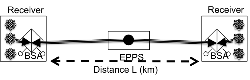
The trial rate of entangling qubits is higher than the other two link architectures, but the success probability is lower.

3.4 Quantum data link protocol

Dahlberg et al. introduced a quantum data link protocol, and analyzed its performance over a detailed network simulation composed of a few qubits, executed on a supercomputer [2019arXiv190309778D]. The required functionality for each layer in the network stack is summarized in Fig. 3.5, and the proposed architecture is shown in Fig. 3.6.

Figure 3.5: Required functionality for each layer network stack as in [2019arXiv190309778D].

Figure 3.6: Layered architecture for quantum communication as in [2019arXiv190309778D].

The higher layer requests quantum state creation of a resource with certain parameters by communicating with the link layer. The Midpoint Heralding Protocol (MHP) periodically asks for triggering entanglement (via polling) to the link layer, and the link layer acknowledges the need with yes/no reply along with some other parameters. There are two types of requests; the Create and Keep (K) request or the Create and Measure (M) request. An example of included parameters in the K request may be the ID, sequence of gate operations, the type of generation and etc. The GEN message is transmitted to the BSA node, and the generation attempt’s success/failure REPLY with its generation ID (which is used by the EGP later) is acknowledged to nodes. This information will also be forwarded to the link layer. The K request specifies the measurement basis, and the qubit is measured along the basis immediately after the photon emission (even before receiving the REPLY message from the BSA node). The measurement result is forwarded to the EGP accordingly.

The Queue in the Entanglement Generation Protocol (EGP) is used for coordinating the MHP triggering timing. The Quantum Memory Management (QMM) tracks which physical qubit is used for which entanglement generation/storing. The Fidelity estimation unit (FEU), based on known hardware capabilities, estimates the minimal completion time for preparing an entangled resource with minimal fidelity $F_{\mbox{min}}$ . The minimal completion time is also used to reject requests from the higher layer based on the given timeout value. The FEU also performs test rounds for improving the estimation. The EGP scheduler manages which request in the queue should be served next.

3.5 Quantum link bootstrapping

Oka et al. discussed procedures for distributed quantum link bootstrapping based on link-level tomography (see Fig. 3.7(a)), and master-slave model based quantum link bootstrapping (see Fig. 3.7(b)), over a MidpointSource link [2016NJPh...18h3015J]. The paper focuses on the accuracy of the reconstructed density matrix (reconstruction fidelity), based on the number of measured Bell pairs. The simulation assumes infinite ideal memories. As shown, both procedures assume the ability to raise the reconstruction fidelity up to a certain threshold.

Figure 3.7: Procedures of quantum link bootstrapping. Here, the fidelity is the reconstruction fidelity. (a) Distributed model. (b) Master-Slave model.

Oka’s bachelor thesis [Oka:Thesis:2017] also considers recurrence purification for increasing the average resource fidelity, over a simulated noisy system with only Pauli errors. The flowchart of the quantum link bootstrapping with recurrence purification is shown in Fig. 3.8. The proposed protocol assumes the ability to raise the reconstruction fidelity and the resource fidelity up to a certain threshold.

Figure 3.8: Procedure of quantum link bootstrapping with purification.

Chapter 4 Protocol Design

This chapter discusses the simulated protocols. The simulation design is made based on the following assumptions.

•

Reliable, in-order timely delivery of classical messages.
•

Paired classical and quantum channels installed between adjacent nodes.
•

Perfectly synchronized clocks.
•

Reliable nodes with no system failures.
•

Nodes capable of determining the length of the quantum channels between neighboring nodes to sufficient accuracy.

4.1 Quantum data link protocol

A quantum repeater requires shared entangled resources between neighboring nodes. The role of the quantum data link protocol is to generate such resources continuously, yet autonomously. This thesis will focus on designing a data link protocol for two closely related repeater link architectures, the MeetInTheMiddle model and the SenderReceiver model (see section 3.3 for details regarding link architectures).

The core concept of the data link protocols introduced in [2016NJPh...18h3015J] will be kept untouched. As in [2016NJPh...18h3015J], this thesis does not elaborate how to synchronize clocks across a network, but will start with the coordination of photon emissions between adjacent nodes.

Supplemental components have been added to the protocol for the network simulation. Coordinating the arrival time of photons at the BSA via messaging between the two nodes with memory is difficult. Instead, the BSA node has been assigned to take responsibility in coordinating the entanglement generation. To start, an activated quantum node classically transmits a Boot Up Notification to all neighboring BSA nodes. For a SenderReceiver link, the sender transmits the message towards the receiver. Once received, the BSA node calculates the photon emission timings and the corresponding burst rate for neighboring nodes, based on the quantum channel lengths and its own single photon detector recovery time. Such information will be classically forwarded to the neighboring quantum nodes to start the entanglement generation. The quantum nodes also need to classically notify the BSA node of the end of the burst. Reception triggers the BSA to recalculate the emission timing for the next round, and returns the information together with a list of success/failure for transmission $i$ , and node addresses specifying between which nodes the resources are shared. We buffer the success/failure results, and send them as a single packet to prevent overflowing the classical channel. Details regarding modules are also provided in section 5.1 and in section 5.2. The rule engine also operates qubit emissions for the quantum data link protocol, which is an operation for generating entangled resources (see Figure. 4.1).

Figure 4.1: Flow chart of resource generation. This process is looped to continuously generate new resources. QNIC is Quantum Network Interface Card, RE is Rule Engine, CNT is Controller and BS is Beamsplitter. For details regarding modules, see section 5.1.

4.2 RuleSet-based communication protocol

Coordinated operation is a prerequisite functionality for quantum networking over both the link layer and the network layer [zimmermann1980osi]. When nodes perform a particular operation using pre-shared entangled resources, participants are assumed to perform the correct operation targeting the appropriate resources. Such consistency should not be achieved by exchanging messages with each other, especially over long distances due to the latency incurred. In this section, we introduce the concept of RuleSet for supporting quantum networking, which allows us to synchronize operations over a network with minimal classical message transmission. If a single connection follows a route involving $n$ nodes, the source node requests the destination node to generate $n$ RuleSets, and distributes them to all $n$ nodes respectively (see Fig. 4.2) [van-meter-qirg-quantum-connection-setup-00].

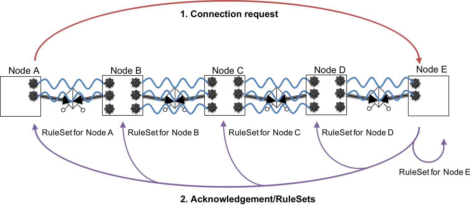
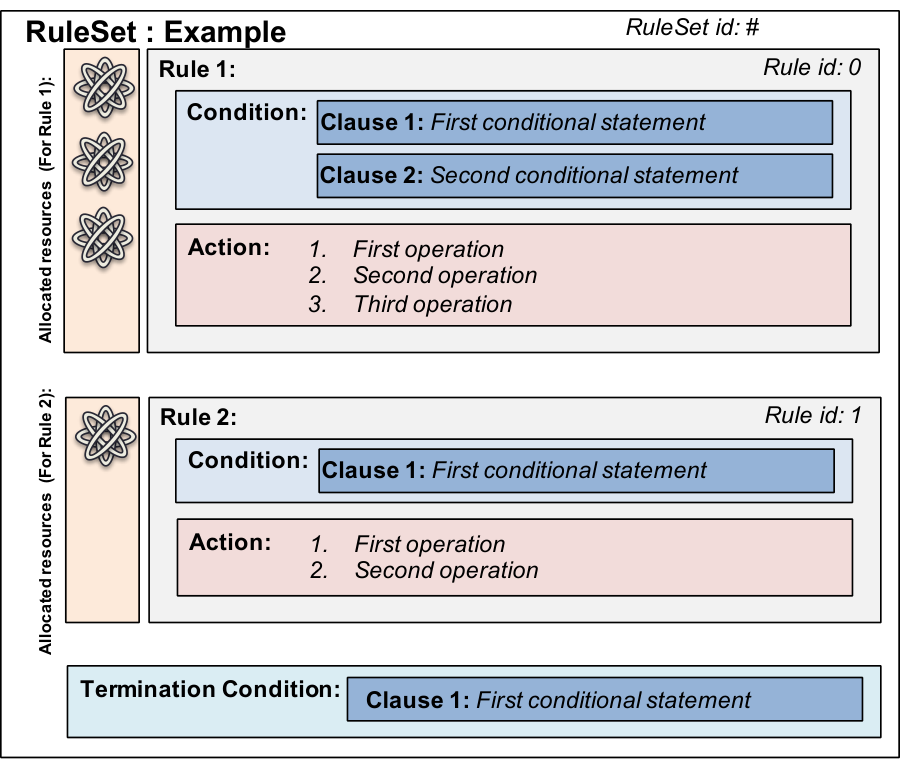
A RuleSet is an object consisting of one or more Rules, each holding a Condition and an Action. A Condition may have one or more Clauses, each of which is a conditional statement. An Action holds a list of operations that a node needs to perform in order to accomplish a single task, which may be for example, entanglement swapping, purification, measurement for tomography, etc., and is invoked if and only if each Clause in the corresponding Condition is fulfilled. When the task involves at least one resource, the oldest available resource will be picked from the allocated set. An Action may also generate a message to another node, lock and reinitialize resources. In our current implementation, a RuleSet also has a Termination Condition, which is a simple counter for determining when to discard the RuleSet and discontinue the connection. This may also have multiple Clauses. Each Rule, also holds more than one partner address, identifying where the paired entangled qubit (or the paired node for a particular operation) is physically located. This is, of course, taken into consideration by the destination node generating the RuleSets for a particular connection.

RuleSets will be managed and executed by the RuleEngine, which is a software module installed in all quantum nodes that is responsible for interpreting the RuleSet instructions, and executing them in real time. The RuleEngine is event-driven, where the event may be a classical packet arrival, new resource allocation or RuleSet timeout. If a single RuleSet consists of multiple Rules, the RuleEngine refers to each Rule based on top-down strategy, invoking Actions from top to bottom sequentially. That is, if a node completes the Action in the first Rule on qubit A, if any, qubit A will be reassigned for the use of the second Rule in the same RuleSet. Therefore, newly generated resources are first assigned to the first Rule in the set, when the generated resource is shared between the partner node of thee first Rule. They must complete the first rule before being reassigned to the second Rule. Timeout may be performed by tracking how well resources are upgraded to the upper Rules. This RuleSet level resource allocation can be directly translated into multiplexing schemes, such as buffer space multiplexing [Aparicio2011]. This top-down approach is also a simple solution to overcome the bias in knowledge regarding the resources across a network (see Fig. 4.3).

All RuleSets for the same connection share the same RuleSet identifier (RuleSetID). The RuleSet identifier is generated via a hash function using the time when the RuleSet was generated, the IP address of the node which generated the RuleSet, and a random number as a seed to avoid global conflicts. Rules are also indexed (RuleID) inside the RuleSet. Each Action holds a counter (ActionIndex), where the counter is incremented whenever the Action has been performed. These identifiers are used, for example, when a node needs to share the measurement result with another node for link-level tomography. Whenever an Action of a RuleSet requires a node to transmit a classical packet to another node, such as the measurement result, it encloses the identifiers in the packet, so that the receiving node can uniquely identify and pair its own measurement result with the received one accordingly. An example structure of a RuleSet composed of two Rules is shown in Fig. 4.4.

When a RuleEngine executes an Action, the Action generally demands one or more entangled resources from its allocated list. Resources are always picked from the oldest, so that operations are performed consistently between the partner node(s). The flow chart of the RuleSet-based quantum link bootstrapping protocol is shown in Figugre.4.5.

Figure 4.5: Flow chart of the hardware monitor working on link-level tomography. RD is Routing Daemon, HM is Hardware Monitor and RE is Rule Engine. For details regarding modules, see section 5.1.

4.3 Pseudocode of Rules

This subsection provides examples of Rules.

4.3.1 Single selection-Single error Purification (Ss-Sp) Rule

The Ss-Sp is the simplest method to detect either the X error or the Z error (see Fig. in section for the circuit).

Condition

The Condition for the Ss-Sp Rule requires a single Clause, which is the ResourceConditionClause shown in Algorithm. 1. This Clause’s role is to check the number of available resources, where $numRequired=2$ in this case. A resource is locked when it should not be disturbed – e.g. waiting for purification result.

Algorithm 1 ResourceConditionClause

1: This Clause checks if enough resources are available for the corresponding Action.

2: Input: resourceList

\leftarrow

List of allocated resources for the Rule. A resource may be locked when it is waiting for the classical packet to arrive, such as for purification.

3: Output: enoughResources

\leftarrow

A boolean value.

5: procedure ResourceConditionClause(resourceList)

6: numRequired

\leftarrow

Number of required resources for the Action

7: numFree

=0

8: enoughResources

=

false

9: for each resource in resourceList do

10: if resource is not locked then

11: numFree

++

12: end if

13: if numFree

>=

numRequired then

14: enoughResources

=

true

15: break

16: end if

17: end for

18: return enoughResources

19: end procedure

Action

The Action for the Ss-Sp Rule simply picks two available resources, and performs an X purification. The purified resource will be locked until the node gets the paired measurement result from the other node.

Algorithm 2 Ss-SpAction

1: This Action performs an X error purification based on single selection. The measurement result is stored, and then sent to the partner node as a message.

2: Input: resourceList

\leftarrow

List of allocated resources for the Rule.

3: Output: msg

\leftarrow

A message for another node.

5: ResourceConditionClause == true

6: procedure Ss-SpAction(resourceList)

7: self_addr

\leftarrow

Node address of this RuleSet owner.

8: partner_addr

\leftarrow

Node address of tomography partner.

9: resource1 = Select a free resource from resourceList

10: resource2 = Select another free resource from resourceList

11: resource2.CNOT(resource1) /*Target.CNOT(Controlled)*/

12: basis = Z

13: outcome = resource2.Measure(basis)

14: removeResourceFromList(resourceList,resource2)

15: lockResourceInList(resourceList,resource1)

16: Data.result = {outcome, basis}

17: Data.ruleSetId = this.RuleSetID

18: Data.ruleId = this.RuleID

19: Data.actionIndex = this.ActionIndex

20: save(Data)

21: msg.destination = partner_addr

22: msg.source = self_addr

23: msg.data = Data

24: this.ActionIndex

++

25: return msg

26: end procedure

Each node will exchange its measurement outcome. The locked resource will only be unlocked and reassigned to the next Rule when the measurement outcomes coincide. Otherwise, purification failed and the locked resource is removed from the resourceList and returned to the pool of unused resources for reinitialization and reuse.

4.3.2 Double selection-Single error Purification (Ds-Sp) Rule

The Ds-Sp is a purification method similar to Ss-Sp but with double selection (see Fig. in section for the circuit) [fujii:PhysRevA.80.042308].

Condition

The only Clause required for the Ds-Sp Rule is also the ResourceConditionClause (see Algorithm. 1 above).

Action

The Action for the Ds-Sp Rule picks three available resources, and performs an X purification based on double selection. The purified resource will be locked until the node gets the paired measurement result from the other node.

Algorithm 3 Ds-SpAction

1: This Action performs an X error purification based on double selection. The measurement result is stored, and then sent to the partner node as a message.

2: Input: resourceList

\leftarrow

List of allocated resources for the Rule.

3: Output: msg

\leftarrow

A message for another node.

5: ResourceConditionClause == true

6: procedure Ds-SpAction(resourceList)

7: self_addr

\leftarrow

Node address of this RuleSet owner.

8: partner_addr

\leftarrow

Node address of tomography partner.

9: resource1 = Select a free resource from resourceList

10: resource2 = Select another free resource from resourceList

11: resource3 = Select another free resource from resourceList

12: resource2.CNOT(resource1) /*Target.CNOT(Controlled)*/

13: resource2.CNOT(resource3) /*Target.CNOT(Controlled)*/

14: resource3.H()

15: basis = Z

16: outcome1 = resource2.Measure(basis)

17: outcome2 = resource3.Measure(basis)

18: removeResourceFromList(resourceList,resource2)

19: removeResourceFromList(resourceList,resource3)

20: lockResourceInList(resourceList,resource1)

21: Data.result = {{outcome1, basis},{outcome2, basis}}

22: Data.ruleSetId = this.RuleSetID

23: Data.ruleId = this.RuleID

24: Data.actionIndex = this.ActionIndex

25: save(Data)

26: msg.destination = partner_addr

27: msg.source = self_addr

28: msg.data = Data

29: this.ActionIndex

++

30: return msg

31: end procedure

Each node will exchange its measurement outcome. The locked resource will only be unlocked when the each of the paired measurement outcomes coincide. Otherwise, purification failed and the locked resource is removed from the resourceList.

4.3.3 Full-state link-level tomography Rule

Condition

The Condition for the tomography Rule requires two Clauses. One of them is the ResourceConditionClause (Algorithm. 1), and another is the MeasurementConditionClause (Algorithm 4). The MeasurementConditionClause is a simple counter for checking the number of measured qubits.

Algorithm 4 MeasurementConditionClause

1: This Clause checks if enough measurements has been performed.

2: Input: none.

3: Output: enoughMeasurements

\leftarrow

A boolean value. True if enough measurements have been performed.

5: procedure MeasurementConditionClause( )

6: numRequired

\leftarrow

Number of required measurements for tomography

7: numCurrent

=0

8: enoughMeasurements

=

false

9: if numCurrent

<

numRequired then

10: numCurrent

++

11: return enoughMeasurements=false

12: else

13: return enoughMeasurements=true

14: end if

15: return enoughMeasurements

16: end procedure

Action

The Action for the tomography selects a qubit, and performs a measurement on it based on a randomly selected basis.

Algorithm 5 TomographyAction

1: This Action performs measurement on an entangled qubit. The measurement result and the selected basis is stored, and sent to the partner node as a message.

2: Input: resourceList

\leftarrow

List of allocated resources for the Rule.

3: Output: msg

\leftarrow

A message for another node.

5: ResourceConditionClause == true && MeasurementConditionClause == true

6: procedure TomographyAction(resourceList)

7: self_addr

\leftarrow

Node address of this RuleSet owner.

8: partner_addr

\leftarrow

Node address of tomography partner.

9: resource = Select a free resource from resourceList

10: basis = RandomBasisSelect({X,Y,Z})

11: outcome = resource.Measure(basis)

12: removeResourceFromList(resourceList,resource)

13: Data.result = {outcome, basis}

14: Data.ruleSetId = this.RuleSetID

15: Data.ruleId = this.RuleID

16: Data.actionIndex = this.ActionIndex

17: save(Data)

18: msg.destination = partner_addr

19: msg.source = self_addr

20: msg.data = Data

21: this.ActionIndex

++

22: return msg

23: end procedure

Selected measurement basis and its outcome will be stored locally, and shared to the partner node.

Chapter 5 Quantum network simulator

The quantum network simulator implemented for this thesis is built on top of a publicly available discrete event network simulator named OMNeT++ [Varga:2008:OOS:1416222.1416290]. OMNeT++ provides users an easy framework for defining network topologies and system area topologies for nodes. Each software/hardware element is defined as a module in OMNeT++, and their functionalities must be programmed by the user. However, some of the basic functions, such as for running Dijkstra’s algorithm (weighted or not), are provided as a standard function. Different classical packets can also be defined very easily as OMNeT++ messages. Simulations are runnable in CUI mode, or in GUI mode with animation.

Because OMNeT++ is a classical networking simulator, components for simulating the physics in quantum networking must be added. Basic mathematics, such as for measuring a qubit with a specific density matrix, have been accomplished though the use of Eigen package [eigenweb]. Physical entanglement of a qubit module has been tracked using a pointer (pointing to another qubit module), and distributed states are directly accessed and updated on demand.

The overall simulator size for this thesis is approximately 10,000 lines of code (see Appendix. ) exclusive of OMNeT++ and Eigen. The following subsections discuss the overall structure of the simulator and its flow. The simulator is designed to evaluate various protocols over a single network, and over the quantum Internet. The Quantum Internet will be a world-wide network interconnecting diverse quantum networks, both small scale and large scale [Kimble2008, VanMeter:2014:QN:2683776, Wehnereaam9288, irtf-qirg-principles-00]. These independent, interconnected networks are utilizing different technologies and managed by different organizations (see Fig. 5.1), known as Autonomous Systems in the classical Internet. The role of such a network is similar to the classical Internet: to provide to users a quantum information service between arbitrary nodes.

5.1 Design of a Quantum node architecture

Building a Quantum network simulator requires designing the hardware/software architecture of a quantum node, which includes end-nodes, quantum repeaters and quantum routers. The challenge is that designing the architecture requires understanding the required module functionalities and protocol specifications across different layers. In our work, we define a node with a single quantum network interface card (QNIC) as an end-node. Similar to the classical network interface card (NIC), the QNIC is connected to another node’s QNIC via a quantum channel. The end-node regularly entangles its own qubits with its neighbor’s. An end-node also generates and transmits a classical connection setup request to another end-node through the classical channel. A node with two QNICs is a quantum repeater. The role of a quantum repeater is to forward classical packets, to create base-level entanglement over a link and to monitor and manage errors. The third type of nodes are the quantum routers, which have similar roles to quantum repeaters, but also takes responsibility for routing, for both classical and quantum information. A border quantum router, which is a router connected to another border quantum router of a different network, may have minimum trust between networks – a router may have no knowledge of the internals of other autonomous networks. Backbone routers also physically and logically link heterogenous networks. Below is the architecture of the simplest quantum node, which is the end-node (see Fig. 5.2) – a quantum repeater or a quantum router has the same architecture, except for the number of QNICs and its need to correctly route packets. Note that the required hardware/software still varies depending on the design decisions. The design is intended for enabling the RuleSet-based communication protocol.

Figure 5.2: Quantum node architecture.

5.1.1 Network Interface Card (NIC)

A NIC is connected to the classical channel, and is capable of forwarding classical packets out to the channel.

Assumption: All NICs are connected to ideal classical channels – no error and infinite bandwidth and the same latency as corresponding QNICs.

5.1.2 Quantum Network Interface Card (QNIC)

A QNIC is connected to the quantum channel. This module contains multiple quantum memories, each capable of emitting one entangled photon out to the channel through the multiplexer (MUX).

Assumption: The simulation assumes the ability to perform any multi-qubit operations between qubits in any local QNICs. The error rate of a particular quantum gate can be set on a node-by-node basis but is fixed throughout the simulation. Gate times are assumed to be negligible.

5.1.3 Application module

The application generates the connection setup request to an arbitrary end-node, and passes the request to the connection manager. The connection setup request may include the required number of Bell-pairs and their minimum fidelity for the application. This module may directly be controlled by a user.

5.1.4 Hardware Monitor

The hardware monitor knows which local QNIC is connected to which neighboring node. An example of the table is shown below in Tab. 5.1.

Table 5.1: Example of a table keeping the pair of the local QNIC id and its connected neighbor address. Neighboring nodes of Node 1 are assumed to be Node 2, 3 and 4

Next hop	QNIC id
Node 2	QNIC 0
Node 3	QNIC 1
Node 4	QNIC 2

Its major role is to monitor and update the states of quantum links (up or down), by generating a request for checking the link quality based on tomography. When received a request, the hardware monitor also generates a RuleSet for the link monitoring. Based on the accumulated measurement results (basis and outcome), the hardware monitor reconstructs the density matrix based on a given algorithm (for details regarding the full-state reconstruction, see Sec. 2.8.4). The acquired link information may be stored by the node as in Tab. 5.2.

Table 5.2: Example of a table keeping the link fidelity and the link throughout information.

QNIC id	Fidelity	Throughput (Bell pairs per second)
QNIC 0	0.88	3312
QNIC 1	0.89	10011
QNIC 2	0.93	5504

The estimated link quality is then provided to the local routing daemon. The overall flow of the process has been provided in Figure .4.5 in section 4.2.

Assumption: The hardware monitor is assumed to be able to access to the exact length of the channels.

5.1.5 Routing Daemon

The routing daemon communicates with the neighbors to exchange the link state information received from the hardware monitor. The module accumulates all node/link information in a single network, and creates a quantum routing table based on a predefined algorithm (e.g. Dijkstra’s algorithm [VanMeter2013]). This daemon, like its classical counterpart, can theoretically support a variety of routing protocols, whether link state, distance vector, or other. The BSA node is not visible in the routing system because the BSA can be considered as a part of the physical link. The message exchange timing diagram with three nodes is provided in Fig. 5.3.

Figure 5.3: Message exchange of the routing daemon exchanging link qualities. RD is Routing Daemon and HM is Hardware Monitor. Link quality may include the achievable fidelity with its corresponding throughput.

A quantum routing table is distinct from the classical routing table, but the overall structure and use remains the same (see Tab. 5.3). The corresponding example topolpogy is shown in Fig.5.4.

Table 5.3: Example quantum routing table of Node 1. A node only knows which neighbor to communicate with. Neighboring nodes of Node 1 are assumed to be Node 2, 3 and 4

Destination	Next hop
Node 2	Node 2
Node 3	Node 3
Node 4	Node 4
Node 5	Node 2
Node 6	Node 3

5.1.6 Connection Manager

The connection manager forwards the connection setup packet to the next quantum node by referring to the quantum routing Tab. The destination node creates the rule set for a particular connection, and distributes it back to all involving nodes (see Fig. 5.5). A RuleSet consists of multiple Rules, each with an Action and a Condition. The Action is a set of operations for accomplishing a single task, and the Condition tells when to execute it. For details, see Sec. 4.2.

Figure 5.5: Flow chart of the connection setup including three nodes. RE is Rule Engine and CM is the Connection Manager.

5.1.7 Rule Engine

The rule engine is event-driven (e.g. classical packet arrival, new resource allocation or RuleSet timeout). It is responsible for interpreting and executing operations in real time through the real-time controller based on the received RuleSet(s). The rule engine also executes the quantum data link protocol for generating new resources (see Fig. 4.1 in section 4.1). Those newly generated resources are assigned to the running RuleSets by the RuleEngine.

Assumption: Rule engines have perfectly synchronized clocks between nodes. Therefore, for example, each node is capable of transmitting a photon exactly at the desired timing.

5.1.8 Real-time Controller

The real-time controller has direct access to all local QNICs and their stationary qubits. Quantum operation, such as qubit measurement, is accomplished through this module ¹¹ 1 In the simulator, however, the Rule Engine directly executes the function of an Action..

5.2 Design of a Bell State Analyzer (BSA) node/module architecture

Below is the architecture of a BSA node (see Fig. 5.6). The BSA is installed in between two nodes along the quantum channel for a MeetInTheMiddle link, or is directly installed at one endpoint’s QNIC for a SenderReceiver link. This node’s main role is to coordinate the resource generations of neighboring nodes.

Figure 5.6: BSA node architecture. Classical communications, shown as dashed arrows, will be sent through the classical channel via NICs.

5.2.1 Beamsplitter & Photon detectors

Optical qubits arrive at the beamsplitter from QNICs via quantum channels. The beamsplitter with its detectors’ role is to perform Bell measurements on the received qubits to stochastically generate entangled resources. The two detectors’ results will be forwarded to the controller module. The first step is to establish that photons can be made indistinguishable from the two nodes. This is confirmed using a Hong-Ou-Mandel test. Then hardware parameters are adjusted to erase the which-path information while detecting photons at both detectors.

5.2.2 Controller

The controller calculates the emission timings for both nodes, and also forwards the accumulated success/failure results.

Assumption: The controller also assumes that each node has the ability to emit photons at the exact timing provided.

5.3 Simulating errors

The error evolution is modeled based on Markov-Chain Monte-Carlo simulation.

5.3.1 Noisy memory errors

When a qubit is waiting for some time $t$ since its initialization, we may observe an error on that qubit. The simulator uses a row vector to describe the present state of a qubit, which is one of the seven distinguishable states – no error, X error, Z error, Y error, excited, relaxed or completely mixed. For example, a Bell pair with no error as an initial input state can be described as in Eq. .

Chapter 1 Introduction

1.1 Background

1.2 Research Contribution

1.3 Thesis structure

Chapter 2 Theory of Quantum Information11 1 Adapted from my bachelor’s thesis, ”Analysis of Measurement-based Quantum Network Coding over Repeater Networks under Noisy Conditions”, Faculty of Environment and Information Studies, Keio University, 2017.

2.1 Historical background of Quantum Computation

2.2 Qubit

2.2.1 Dirac notation

2.2.2 Bloch sphere

2.2.3 Eigenvalue and Eigenvector

2.3 Composite quantum systems

2.4 Quantum Gates

2.4.1 Single Qubit Gates

2.4.2 Measurement in a circuit

Measuring a qubit

2.4.3 Controlled Gates

2.5 Alternative state representations

2.5.1 Density matrix and Mixed States

Calculating the density matrix of a left-over system after a measurement

2.5.2 Stabilizer

2.6 Entanglement

2.6.1 Bell pair/Einstein-Podolsky-Rosen (EPR) pair

2.6.2 W state

2.6.3 Greenberger-Horne-Zeilinger (GHZ) state

2.6.4 Cluster state

2.7 Reading quantum circuits

2.7.1 Understanding circuits using matrices

Step 1

Step 2

Step 3

Other cases

2.7.2 Understanding circuits using stabilizers

Step 1

Step 2

Step 3

2.8 Quantum networking

2.8.1 Quantum Teleportation

2.8.2 Entanglement Swapping

2.8.3 Entanglement Purification

2.8.4 Quantum state tomography

Single qubit tomography using projective measurements

Two-qubit tomography using projective measurements

2.8.5 Verification of quantum correlation (entangled states) via CHSH inequality

2.8.6 Quantum Repeaters

2.8.7 Generations of Network Evolution

2.9 Errors on quantum systems and its measure

2.9.1 Error

Pauli errors

Propagation of Pauli errors

Other unfixable errors

2.9.2 Fidelity

2.10 Measurement-based Quantum Computing

Chapter 3 Related Work

3.1 Violation of a Bell inequality

3.2 Long range entanglement distribution

3.3 Physical link architecture

3.3.1 MeetInTheMiddle

3.3.2 SenderReceiver

3.3.3 MidpointSource

3.4 Quantum data link protocol

3.5 Quantum link bootstrapping

Chapter 4 Protocol Design

4.1 Quantum data link protocol

4.2 RuleSet-based communication protocol

4.3 Pseudocode of Rules

4.3.1 Single selection-Single error Purification (Ss-Sp) Rule

Condition

Action

4.3.2 Double selection-Single error Purification (Ds-Sp) Rule

Condition

Action

4.3.3 Full-state link-level tomography Rule

Condition

Action

Chapter 5 Quantum network simulator

5.1 Design of a Quantum node architecture

5.1.1 Network Interface Card (NIC)

5.1.2 Quantum Network Interface Card (QNIC)

5.1.3 Application module

5.1.4 Hardware Monitor

Chapter 2 Theory of Quantum Information¹¹ 1 Adapted from my bachelor’s thesis, ”Analysis of Measurement-based Quantum Network Coding over Repeater Networks under Noisy Conditions”, Faculty of Environment and Information Studies, Keio University, 2017.