Intelligent Reflecting Surface-Assisted Millimeter Wave Communications: Joint Active and Passive Precoding Design
Abstract
Millimeter wave (MmWave) communications is capable of supporting multi-gigabit wireless access thanks to its abundant spectrum resource. However, severe path loss and high directivity make it vulnerable to blockage events, which can be frequent in indoor and dense urban environments. To address this issue, in this paper, we introduce intelligent reflecting surface (IRS) as a new technology to provide effective reflected paths to enhance the coverage of mmWave signals. In this framework, we study joint active and passive precoding design for IRS-assisted mmWave systems, where multiple IRSs are deployed to assist the data transmission from a base station (BS) to a single-antenna receiver. Our objective is to maximize the received signal power by jointly optimizing the BS’s transmit precoding vector and IRSs’ phase shift coefficients. Although such an optimization problem is generally non-convex, we show that, by exploiting some important characteristics of mmWave channels, an optimal closed-form solution can be derived for the single IRS case and a near-optimal analytical solution can be obtained for the multi-IRS case. Our analysis reveals that the received signal power increases quadratically with the number of reflecting elements for both the single IRS and multi-IRS cases. Simulation results are included to verify the optimality and near-optimality of our proposed solutions. Results also show that IRSs can help create effective virtual line-of-sight (LOS) paths and thus substantially improve robustness against blockages in mmWave communications.
Index Terms:
Intelligent reflecting surfaces (IRS)-assisted mmWave systems, joint active and passive precoding design.I Introduction
Millimeter-wave (mmWave) communication is a promising technology for future cellular networks [1, 2, 3]. It has the potential to offer gigabits-per-second communication data rates by exploiting the large bandwidth available at mmWave frequencies. A key challenge for mmWave communication is that signals experience a much more significant path loss over mmWave frequency bands as compared with the path attenuation over lower frequency bands [4]. To compensate for the severe path loss in mmWave systems, large antenna arrays are generally used to achieve significant beamforming gains for data transmission [5, 6, 7]. On the other hand, high directivity makes mmWave communications vulnerable to blockage, which can be frequent in indoor and dense urban environments. For instance, due to the narrow beamwidth of mmWave signals, a very small obstacle, such as a person’s arm, can effectively block the link [8]. To address this issue, in some prior works, e.g. [9, 10, 11], relays are employed to overcome blockage and improve the coverage of mmWave signals.
Recently, to address the blockage issue and enable indoor mobile mmWave networks, reconfigurable reflect-arrays (also referred to as intelligent reflecting surfaces) were introduced to establish robust mmWave connections for indoor networks even when the line-of-sight (LOS) link is blocked by obstructions, and the proposed solution was validated by a test-bed with reflector units [12]. Intelligent reflecting surface (IRS) has been recently proposed as a promising new technology for realizing a smart and programmable wireless propagation environment via software-controlled reflection [13, 14]. Specifically, IRS, made of a newly developed metamaterial, is a planar array comprising a large number of reconfigurable passive elements. With the aid of a smart micro controller, each element can independently reflect the incident signal with a reconfigurable amplitude and phase shift. By properly adjusting the phase shifts of the passive elements, the reflected signals can add coherently at the desired receiver to improve the signal power or destructively at non-intended receivers to suppress interference [15].
IRS-aided wireless communications have attracted much attention recently [16, 15, 17, 18, 19, 20, 21, 22, 23]. A key problem for IRS-aided systems is to jointly optimize the active beamforming vector at the BS and the reflection coefficients at the IRS to achieve different objectives. Such a problem was studied in a single-user scenario, where the objective was to maximize the receive signal power [16]. A similar problem was considered in an orthogonal frequency division multiplexing (OFDM)-based communication system [18], with the objective of maximizing the achievable rate. In addition, the joint BS-IRS optimization problem was investigated in a downlink multi-user scenario, e.g. [19, 20, 21]. In [24, 25, 26, 27, 28, 29, 30], IRS was also considered as an auxiliary facility to assist secret communications, unmanned aerial vehicle (UAV) communications and wireless power transfer. In [31], the joint beamforming problem was studied to maximize the capacity of an IRS-assisted MIMO indoor mmWave system.
Inspired by encouraging results reported in [12], in this paper, we consider a scenario where multiple IRSs are deployed to assist downlink point-to-point mmWave communications. A joint active and passive precoding design problem is studied, where the objective is to maximize the received signal power by jointly optimizing the BS’s transmit precoding vector and IRSs’ phase shift coefficients. Note that such a joint active and passive precoding problem is non-convex and has been studied in previous works [16, 15] for conventional microwave communication systems, where a single IRS is deployed to assist the data transmission from the BS to the user. In [16], this non-convex problem was relaxed as a convex semidefinite programming (SDP) problem. Nevertheless, the proposed approach is sub-optimal and does not have an analytical solution. In addition, solving the SDP problem usually involves a high computational complexity.
In this paper, we will revisit this joint active and passive beamforming problem from a mmWave communication perspective. We show that, by exploiting some inherent characteristics of mmWave channels, in particular an approximately rank-one structure of the BS-IRS channel, an optimal closed-form solution can be derived for the single IRS case and a near-optimal analytical solution can be obtained for the multi-IRS case. Based on the analytical solutions, we derive the maximum achievable average received power, which helps gain insight into the effect of different system parameters, including the number of passive reflecting elements and the transmitter’s antennas, on the system performance. Our work focuses on a single data stream transmission from the BS to the user. Although it is desirable to exploit point-to-point multi-stream communications in order to improve the spectral efficiency and achieve high data rates, there are still some important scenarios where only a single-stream transmission is available due to the rank-deficiency of the cascade channel between the BS and the UE, or due to the use of a single antenna/RF chain at the UE. In particular, mmWave has limited diffraction and reflection abilities. Hence, multi-stream mmWave communications may not be available for some indoor or outdoor environments where the propagation is dominated by the LOS component.
We noticed that the joint active and passive beamforming problem for multi-user mmWave systems was studied in [32], where a sophisticated gradient-projection (GP) method was developed. Nevertheless, due to the complex nature of the problem, no analytical solution is available for the multi-user scenario. In this case, the performance gain brought by the IRS has to be demonstrated through numerical results as conducting a theoretical analysis of the system performance is rather difficult.
The rest of the paper is organized as follows. In Section II, the system model and the joint active and passive precoding problem are discussed. The joint active and passive precoding problem with a single IRS is studied in Section III, where a closed-form optimal solution is developed and the average received power is analyzed. The joint active and passive precoding problem with multiple IRSs is then studied in Section IV, where a near-optimal analytical solution is proposed. The extension of our proposed solution to low-resolution phase shifters is discussed in Section V. Simulation results are presented in Section VI, followed by concluding remarks in Section VII.
II System Model and Problem Formulation
We consider an IRS-assisted mmWave downlink system as illustrated in Fig.1, where multiple IRSs are deployed to assist the data transmission from the BS to a single-antenna user. Suppose IRSs are employed to enhance the BS-user link, and the number of reflecting units at each IRS is denoted by . The BS is equipped with antennas. Let denote the channel from the BS to the user, denote the channel from the BS to the th IRS, and denote the channel from the th IRS to the user. Each element on the IRS behaves like a single physical point which combines all the received signals and then re-scatters the combined signal with a certain phase shift [16]. Let denote the phase shift associated with the th passive element of the th IRS. Define
| (1) |
Let denote the precoding/beamforming vector used by the BS. The signal received at the user can then be expressed as
| (2) |
where is the transmitted signal which is modeled as a random variable with zero mean and unit variance, and denotes the additive white Gaussian noise with zero mean and variance . Note that in the above model, signals that are reflected by the IRS two or more times are ignored due to the high path loss of mmWave transmissions. Accordingly, the signal power received at the user is given as
| (3) |

In this paper, we assume that the knowledge of the global channel state information is available. Channel estimation for IRS-assisted systems can be found in, e.g. [33, 34, 35, 36]. In particular, [34, 35, 36] discussed how to estimate the channel for IRS-assisted mmWave systems. We aim to devise the precoding vector and the diagonal phase shift matrices to maximize the received signal power, i.e.
| s.t. | ||||
| (4) |
where denotes the maximum transmit power at the BS. Note that here we only consider the communication power. In practical systems, the computation cost may also need to be considered in order to achieve a good balance between the energy efficiency and the spectral efficiency [37]. Such a tradeoff for IRS-aided mmWave systems is an interesting and important topic worthy of future investigation. The problem (4) is referred to as joint active and passive beamforming. Note that the optimization problem (4) with has been studied in [16], where the nonconvex problem was relaxed as a convex semidefinite programming (SDP) problem. Nevertheless, the proposed approach is generally sub-optimal and does not have an analytical solution. Besides, solving the SDP problem involves a high computational complexity.
In this paper, we will revisit this joint active and passive beamforming problem for mmWave communications by exploiting some inherent characteristics of mmWave channels. Specifically, mmWave channels are typically sparsely-scattered. A widely used Saleh-Valenzuela (SV) channel model for mmWave communications is given as [38, 39, 40]:
| (5) |
where and respectively denote the number of antennas at the transmitter and the receiver, is the total number of paths, is the LOS component with representing the complex gain, representing the angle of arrival at the receiver, and representing the angle of departure at the transmitter, and denotes the th non-line-of-sight (NLOS) component. Also, and denote the array response vectors associated with the receiver and the transmitter, respectively. In addition to the sparse scattering characteristics, many measurement campaigns reveal that the power of the mmWave LOS path is much higher (about 13dB higher) than the sum of power of NLOS paths [41, 42]. Hence, any system that is not centered around the transmission via the direct LOS path usually gives only limited gains [31]. Motivated by this fact, it is highly desirable to ensure that the channel between the BS and each IRS is LOS dominated. In practice, with the knowledge of the location of the BS, IRSs can be installed within sight of the BS. Since the power of NLOS paths is negligible compared to that of the LOS path, the BS-IRS channel can be well approximated as a rank-one matrix, i.e.
| (6) |
where is a scaling factor accounting for antenna and path gains, and represent the normalized array response vector associated with the IRS and the BS, respectively. As will be shown later in this paper, this rank-one channel structure can be utilized to obtain a closed-form solution to (4). Also, our simulation results show that our proposed solution based on this rank-one approximation can achieve a received signal power that is nearly the same as that attained by taking those NLOS paths into account.
III Joint Precoding Design for Single IRS
III-A Optimal Solution
In this section, we first consider the case where there is only a single IRS, i.e. . We omit the subscript for simplicity in the single IRS case. The optimization (4) is simplified as
| s.t. | ||||
| (7) |
We will show that by exploiting the rank-one structure of the BS-IRS channel matrix , a closed-form solution to (7) can be obtained. Substituting into the objective function of (7), we obtain
| (8) |
where in , we define , , denotes the Hadamard (elementwise) product, and
| (9) |
in , we write , and the inequality becomes an equality when the arguments (also referred to as phases) of the two complex numbers and are identical. It should be noted that we can always find an such that the arguments of and are identical, although at this point we do not know the exact value of . Therefore the optimization (7) can be rewritten as
| s.t. | (10) |
It is clear that the optimization of is independent of , and can be solved via
| s.t. | (11) |
It can be easily verified that the objective function reaches its maximum when
| (12) |
where denotes the argument of the complex number , and denotes the th entry of .
So far we have obtained the optimal solution of , which, as analyzed above, is independent of the optimization variables and . Based on this result, the optimization (7) can be simplified as
| s.t. | (13) |
where . For a fixed , it is clear that the optimal precoding vector , also known as the maximum ratio transmission (MRT) solution, is given by
| (14) |
By substituting the optimal precoding vector into (13), the problem becomes optimization of :
| (15) |
whose optimal solution can be easily obtained as
| (16) |
where the last equality follows from the fact that is a real-valued number. After the optimal value of is obtained, the optimal precoding vector can be determined by substituting (16) into (14), and the optimal diagonal phase shift matrix is given as
| (17) |
We see that under the rank-one BS-IRS channel assumption, a closed-form solution to the joint active and passive beamforming problem (7) can be derived. To calculate this optimal solution, we only need to compute and , which involves a computational complexity of .
III-B Power Scaling Law
We now characterize the scaling law of the average received power with respect to the number of reflecting elements . For simplicity, we set . Our main results are summarized as follows.
Proposition 1
Assume , , and the BS-IRS channel is characterized by a rank-one geometric model given as
| (18) |
where denotes the complex gain associated with the LOS path between the BS and the IRS, and are normalized array response vectors associated with the IRS and the BS, respectively. Then the average received power at the user attained by the optimal solution of (7) is given as
| (19) |
Proof:
See Appendix A. ∎
From (19), we see that the average received signal power attained by the optimal beamforming solution scales quadratically with the number of reflecting elements . Such a “squared improvement” is due to the fact that the optimal beamforming solution not only allows to achieve a transmit beamforming gain of in the IRS-user link, but it also acquires a gain of by coherently collecting signals in the BS-IRS link. This result implies that scaling up the number of reflecting elements is a promising way to compensate for the significant path loss in mmWave wireless communications.
IV Joint Precoding Design for Multiple IRSs
In this section, we return to the joint active and passive beamforming problem (4) for the general multi-IRS setup. Such a problem is more challenging as we need to jointly design the precoding vector and a set of phase shift matrices associated with IRSs. In the following, by exploiting the rank-one structure of BS-IRS channels and the near-orthogonality between array response vectors, we show that a near-optimal analytical solution can be obtained for this nonconvex problem.
IV-A Proposed Solution
Substituting into the objective function of (4), we arrive at
| (20) |
where in , we define , , and , in , we write , and the inequality becomes an equality when the arguments (or phases) of all complex numbers inside the brackets of are identical. It should be noted that there exist a set of such that the arguments of and are identical, although at this point we do not know the values of . Therefore (4) is equivalent to maximizing the upper bound given in (20), i.e.
| s.t. | (21) |
From (21), it is clear that the optimization of can be decomposed into a number of independent sub-problems, with solved by
| s.t. | (22) |
It can be easily verified that the objective function reaches its maximum when
| (23) |
where denotes the th entry of .
So far we have obtained the optimal solution of , which, as analyzed above, is independent of the optimization variables and . Based on this result, the optimization (4) can be reformulated as
| s.t. | (24) |
where . Note that
| (25) |
is a real-valued number. Thus the objective function of (24) can be written in a more compact form as
| (26) |
where in , we define , and , and in , we define . Hence (24) can be simplified as
| s.t. | (27) |
Note that for any given , an optimal precoding vector , i.e. the MRT solution, is given as
| (28) |
Substituting the optimal precoding vector into the objective function of (27) yields
| s.t. | (29) |
or equivalently,
| s.t. | (30) |
Due to the unit circle constraint placed on entries of , the above optimization (30) is non-convex. In the following, we first develop a sub-optimal semidefinite relaxation (SDR)-based method to solve (30). Then, we show that by utilizing the near-orthogonality among array response vectors, a near-optimal analytical solution of (30) can be obtained.
IV-A1 A SDR-Based Approach for Solving (30)
Note that (30) is a non-convex quadratically constrained quadratic program (QCQP), which can be reformulated as a homogeneous QCQP by introducing an auxiliary variable :
| s.t. | (31) |
where
and denotes the th entry of . Note that , where is a rank-one and positive semidefinite matrix, i.e. . Relaxing the rank-one constraint, the problem (31) becomes
| s.t. | ||||
| (32) |
where denotes the th diagonal element of . The problem above is a standard convex semidefinite program (SDP) which can be solved by convex tools such as CVX. It can be readily verified that the computational complexity for solving (32) is at the order of . In general, the optimal solution of (32) is not guaranteed to be a rank-one matrix. To obtain a rank-one solution from the obtained higher-rank solution of (32), one can follow the steps described in [43].
IV-A2 Near-Optimal Analytical Solution To (30)
The SDR-based method discussed above does not yield a closed-form solution and is computationally expensive. In the following, we propose a near-optimal analytical solution to (30) via utilizing the near-orthogonality among different steering vectors .
Suppose a uniform linear array is employed at the BS. It can be easily verified that the inner product of the two distinct array response vectors and is given as
| (33) |
where
| (34) |
in which denotes the distance between neighboring antenna elements, is the signal wavelength, and denotes the angle of departure associated with the array response vector . It is clear that
| (35) |
In [44], it was shown that asymptotic orthogonality still holds for uniform rectangular arrays. Due to the small wavelength at the mmWave frequencies, the antenna size is very small, which allows a large number (hundreds or thousands) of array elements to be packed into a small area in practical systems. In addition, to improve the coverage, it is expected that different IRSs should be deployed such that they, as seen from the BS, are sufficiently separated in the angular domain, i.e. the angles of departure are sufficiently separated. Taking into account these factors, it is reasonable to assume that different steering vectors are near-orthogonal to each other, i.e. . Therefore we have
| (36) |
which is a constant independent of the vector . Consequently, the optimization (30) can be simplified as
| s.t. | (37) |
It can be easily verified that the optimal solution to (37) is given by
| (38) |
where , and denotes the th entry of . After the near-optimal phase vector is obtained, it can be substituted into (28) to obtain the precoding vector . Also, the near-optimal diagonal phase shift matrix associated with the th IRS is given by
| (39) |
where is the th entry of . To calculate this near-optimal analytical solution, the dominant operation includes calculating and , which has a computational complexity of the order .
IV-B Power Scaling Law
We now analyze the scaling law of the average received power in the general multi-IRS setup with respect to the number of passive elements . Again, we set for simplicity. Our main results are summarized as follows.
Proposition 2
Assume , , and the BS-IRS channel is characterized by a rank-one geometric model given as
| (40) |
where denotes the complex gain associated with the LOS path between the BS and the th IRS, and are normalized array response vectors associated with the IRS and the BS, respectively. Then the average received power attained by the near-optimal analytical solution is given by
| (41) |
Proof:
See Appendix B. ∎
We see that, similar to the single IRS case, the average received signal power attained by the near-optimal analytical solution scales quadratically with the number of reflecting elements . Also, as expected, the average received signal power is a sum of the received signal power from multiple IRSs, which indicates that better performance can be achieved by deploying multiple IRSs.
V Extension to Discrete Phase Shifts
In previous sections, to simplify our problem, we assume that elements of IRSs have an infinite phase resolution. Nevertheless, due to hardware limitations, the phase shift may not take an arbitrary value, instead, it may have to be chosen from a finite set of discrete values [12, 45]. Specifically, the set of discrete values for the phase shift is defined as
| (42) |
where denotes the resolution of the phase shifter. To meet the finite resolution constraint imposed on the phase shifters, a simple yet effective solution is to let each phase shift, , take on a discrete value that is closest to its optimal (or near-optimal) value obtained in previous sections, i.e.
| (43) |
where denotes the th diagonal entry of . In the following, we analyze the impact of the phase discretization on the system performance. Let
| (44) |
denote the average received power attained by our solution with -bit phase shifters, where with given by (43). Without loss of generality, we assume the transmit signal power . Our main results are summarized as follows.
Proposition 3
Assume , and the BS-th IRS channel is characterized by (6). As , we have
| (45) |
It is not difficult to verify that increases monotonically with and approaches as .
Proof:
See Appendix C. ∎
This proposition provides a quantitative analysis of the average received signal power in the multiple-IRS assisted system with discrete phases shifts. We see that, when compared with the receive power achieved by IRSs with infinite-resolution phase shifters, the receive signal power attained by our proposed solution decreases by a constant factor that depends on the number of quantization levels . Specifically, we have , and . Note that a similar result was also reported in [45]. Nevertheless, the result in [45] is derived by considering a simple scenario where both the transmitter and the receiver are equipped with a single antenna. The extension of the result in [45] to the multiple transmit antenna scenario is not straightforward. Also, in [45], only a single IRS is employed, whereas our work considers a more general case where multiple IRS are deployed to assist the downlink communication.
VI Simulation Results
We now present simulation results to illustrate the performance of the proposed IRS-assisted precoding solutions. In our simulations, we consider a scenario where the BS employs a ULA with antennas, and each IRS consists of a uniform rectangular array (URA) with reflecting elements, in which and denote the number of elements along the horizontal axis and vertical axis, respectively. The BS-user channel is generated according to the following geometric channel model [38]:
| (46) |
where is the number of paths, is the complex gain associated with the th path, is the associated angle of departure, represents the normalized transmit array response vector. The complex gain is generated according to a complex Gaussian distribution [40]
| (47) |
with given as
| (48) |
in which denotes the distance between the transmitter and the receiver, and . The values of , are set to be , , and dB, as suggested by real-world NLOS channel measurements [40].
The IRS-user channel and the BS-IRS channel are generated according the aforementioned geometric SV model in LOS scenarios. Specifically, the IRS-user channel is denoted by
| (49) |
where is the number of paths, denotes the complex gain associated with the LOS component, is the complex gain associated with the th NLOS path, () denotes the azimuth (elevation) angle of departure associated with the IRS-user path, represents the normalized transmit array response vector.
On the other hand, the BS-IRS channel is characterized by the SV channel model given as
| (50) |
where denotes the complex gain with the LOS component, () denotes the azimuth (elevation) angle of arrival associated with th NLOS path, is the associated angle of departure, and represent the normalized receive and transmit array response vectors, respectively. The complex gain and are generated according to (47). The values of , are set to be , , and dB as suggested by LOS real-world channel measurements [40]. The Rician factor (defined as as the ratio of the energy in the LOS path to the sum of the energy in other NLOS paths) is set to be dB according to [41]. Also, unless specified otherwise, we assume , , and in our experiments. Other parameters are set as follows: dBm, dBm. The average receive SNR is defined as , where is the received signal power. Since the noise power is fixed, the difference between the average receive SNR and the average received signal power is a constant. All results are averaged over random channel realizations.
VI-A Results for Single IRS
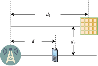
We consider a setup where the IRS lies on a horizontal line which is in parallel to the line that connects the BS and the user (Fig. 2). The horizontal distance between the BS and the IRS is set to meters and the vertical distance between two lines is set to meters. Let denote the distance between the BS and the user. The BS-IRS distance and the IRS-user distance can then be respectively calculated as and .
Fig. 3 plots the average receive SNRs of our proposed solutions with both continuous-valued and discrete-valued phase shifts. Note that for our proposed solutions, the BS-IRS channel is approximated as a rank-one channel by ignoring those NLOS paths. The upper bound of the average receive SNR obtained in [16] is included for comparison. Also, to show the benefits brought by IRSs, a conventional system without IRSs is considered, where the optimal MRT solution is employed. We see that our proposed solution with continuous-valued phase shifters nearly achieves the upper bound of the average receive SNR, which verifies the optimality of our proposed closed-form solution and suggests that neglecting the NLOS paths between the BS and the IRS has little impact on the system performance. Also, with 2-bit low-resolution phase shifts, our proposed solution can achieve an average receive SNR close to that attained by assuming infinite-precision phase shifters. Moreover, it is observed that for the system without IRSs, the average receive SNR decreases rapidly as the user moves away from the BS. As a comparison, this issue can be relieved and the signal coverage can be substantially enhanced via the use of IRSs.

In Fig. 4, we plot the average receive SNR versus the number of reflecting elements at the IRS when m, where we fix and increase . From Fig. 4, we observe that the average receive SNR increases quadratically with the number of reflecting elements. Specifically, the difference between the receive SNRs when and is approximately equal to dB, which coincides well with our analysis. In addition, the average receive SNR loss due to the use of low-resolution phase shifters is analyzed and given by (45). Specifically, we have dB and dB. It can be observed that simulation results are consistent with our theoretical result.

VI-B Results for Multiple IRSs
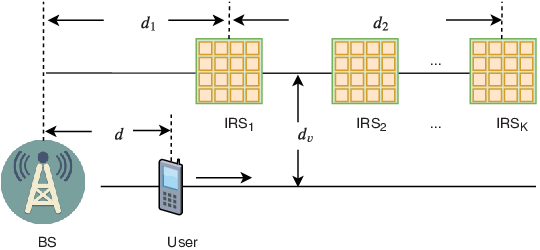
We consider a multi-IRS setup as depicted in Fig. 5, where IRSs are equally spaced on a straight line which is in parallel with the line connecting the BS and the user. Specifically, the horizontal distance between the BS and the first IRS is set to m and the vertical distance is set to m. Also, the distance between the nearest IRS and the farthest IRS is set to be m. We set if not specified otherwise. In this example, the SV channel model used to characterize the BS-IRS channel only contains a LOS component.
Fig. 6 depicts the average receive SNRs attained by our proposed SDR-based approach and the near-optimal analytical solution as a function of the BS-user distance. To verify the effectiveness of the proposed solutions, an upper bound on the average receive SNR is obtained by solving the relaxed SDP problem (32). We see that the curve of the analytical solution almost coincides with the upper bound, which validates the near-optimality of the proposed analytical solution.

In Fig. 7, we plot the average receive SNRs of different schemes versus the number of reflecting elements at each IRS, where we fix and change . It can be observed that the squared improvement also holds true for the near optimal analytical solution. Specifically, when , the receive SNR at the user is approximate to dB, while it increases up to dB when the number of reflecting elements doubles, i.e. . Also, we see that the near-optimal analytical solution achieves an average receive SNR that is closer to the upper bound when becomes larger, which corroborates our claim that our proposed analytical solution is asymptotically optimal when approaches infinity. Also, it can be seen that the receive SNR loss due to discretization coincides well with our analysis.


To show the robustness of the IRS-assisted system against blockages, we calculate the average throughput and the outage probability for our proposed near-optimal analytical solution. The average throughput and the outage probability are respectively defined as
| (51) |
| (52) |
where denotes the required threshold level and set to according to [9]. We assume that the BS-IRS link is always connected. Also, the blockage probabilities of the BS-user link and the IRS-user link are assumed to be the same in our simulations. From Fig. 8(b), we observe that the outage probability can be substantially reduced by deploying IRSs. Also, the more the IRSs are deployed, the lower the outage probability can be achieved. Particularly, when , the outage probability reduces to zero if the link blockage probability is less than . This result shows the effectiveness of IRSs in overcoming the blockage issue that prevents the wider applications of mmWave communications.


VII Conclusions
In this paper, we studied the problem of joint active and passive precoding design for IRS-assisted mmWave systems, where multiple IRSs are deployed to assist the data transmission from the BS to a single antenna user. The objective is to maximize the received signal power by jointly optimizing the transmit precoding vector at the BS and the phase shift parameters user by IRSs for passive beamforming. By exploiting some important characteristics of mmWave channels, we derived a closed-form solution for the single IRS case, and a near-optimal analytical solution for the multi-IRS case. Simulation results were provided to illustrate the optimality and near-optimality of proposed solutions. Our results also showed that IRSs can help create effective virtual LOS paths to improve robustness of mmWave systems against blockages.
Appendix A Proof of Proposition 1
When the optimal active and passive beamforming solution is employed, from (15), we know that the received signal power at the user is given as
| (53) |
where
| (54) |
in which the latter equality comes from the fact that . Therefore we have
| (55) |
We first calculate . Since , the mean and variance of the modulus of th entry of are respectively given as
| (56) | ||||
| (57) |
Thus
| (58) |
Hence can be computed as
| (59) |
and
| (60) |
Therefore is given as
| (61) |
Now let us examine . It is clear that
| (62) |
As a result, we have
| (63) |
and
| (64) |
In addition, it can be easily verified that
| (65) |
Combining (61), (64) and (65), we reach (19). This completes our proof.
Appendix B Proof of Proposition 2
When the analytical active and passive beamforming solution is employed, from (29), we know that the received signal power at the user is given as
| (66) |
where is given by (38), is due to (36), and
| (67) |
Therefore we have
| (68) |
We first calculate . Since , we have
| (69) |
| (70) |
| (71) |
Hence can be computed as
| (72) |
and
| (73) |
Therefore, we have
| (74) |
and
| (75) |
Now we examine . From (38), we arrive
| (76) |
we can verify that
| (77) |
Since is also a random variable, we can calculate as
| (78) |
As a result, we have
| (79) |
Appendix C Proof of Proposition 3
To facilitate our analysis, we rewrite (43) as
| (81) |
where , , in which is the discretization error. By substituting (81) into (44), the average received signal power is given by
| (82) |
where in , we define
| (83) |
in , we define and comes from (36).
Since discrete phase shift values in are uniformly spaced, discretization errors can be considered as independent random variables uniformly distributed on the interval . Thus can be calculated as
| (84) |
in which
| (85) |
Also, can be computed as
| (86) |
References
- [1] T. S. Rappaport, J. N. Murdock, and F. Gutierrez, “State of the art in 60-GHz integrated circuits and systems for wireless communications,” Proc. IEEE, vol. 99, no. 8, pp. 1390–1436, Aug. 2011.
- [2] S. Rangan, T. S. Rappaport, and E. Erkip, “Millimeter-wave cellular wireless networks: potentials and challenges,” Proc. IEEE, vol. 102, no. 3, pp. 366–385, Mar. 2014.
- [3] A. Ghosh, T. A. Thomas, M. C. Cudak, R. Ratasuk, P. Moorut, F. W. Vook, T. S. Rappaport, G. R. MacCartney, S. Sun, and S. Nie, “Millimeter-wave enhanced local area systems: a high-data-rate approach for future wireless networks,” IEEE J. Sel. Areas Commun., vol. 32, no. 6, pp. 1152–1163, Jun. 2014.
- [4] A. L. Swindlehurst, E. Ayanoglu, P. Heydari, and F. Capolino, “Millimeter-wave massive MIMO: the next wireless revolution?” IEEE Commun. Mag., vol. 52, no. 9, pp. 56–62, Sep. 2014.
- [5] A. Alkhateeb, J. Mo, N. Gonzalez-Prelcic, and R. Heath, “MIMO precoding and combining solutions for millimeter-wave systems,” IEEE Commun. Mag., vol. 52, no. 12, pp. 122–131, Dec. 2014.
- [6] A. Li and C. Masouros, “Hybrid analog-digital millimeter-wave MU-MIMO transmission with virtual path selection,” IEEE Commun. Lett., vol. 21, no. 2, pp. 438–441, 2016.
- [7] J. Zhang, X. Ge, Q. Li, M. Guizani, and Y. Zhang, “5G millimeter-wave antenna array: Design and challenges,” IEEE Wireless Commun., vol. 24, no. 2, pp. 106–112, 2016.
- [8] O. Abari, D. Bharadia, A. Duffield, and D. Katabi, “Enabling high-quality untethered virtual reality,” in 14th USENIX Symp. Netw. Syst. Des. and Implementation (NSDI 17). Boston, MA: USENIX Association, Mar. 27-29, 2017, pp. 531–544.
- [9] G. Yang, J. Du, and M. Xiao, “Maximum throughput path selection with random blockage for indoor 60 GHz relay networks,” IEEE Trans. Commun., vol. 63, no. 10, pp. 3511–3524, October 2015.
- [10] S. Zubair, S. Jangsher, Y. Mao, and V. O. K. Li, “Blockage-aware power allocation and relay selection in millimeter-wave small cell network,” in 2019 16th IEEE Annu. Consum. Commun. Netw. Conf. (CCNC), Flamingo LV, Jan. 11-14 2019, pp. 1–5.
- [11] Y. Niu, W. Ding, H. Wu, Y. Li, X. Chen, B. Ai, and Z. Zhong, “Relay-assisted and QoS aware scheduling to overcome blockage in mmwave backhaul networks,” IEEE Trans. Veh. Technol., vol. 68, no. 2, pp. 1733–1744, Feb. 2019.
- [12] X. Tan, Z. Sun, D. Koutsonikolas, and J. M. Jornet, “Enabling indoor mobile millimeter-wave networks based on smart reflect-arrays,” in IEEE Int. Conf. Comput. Commun. (INFOCOM), Honolulu, Hawaii, Apr. 15-19 2018, pp. 270–278.
- [13] T. J. Cui, M. Q. Qi, X. Wan, J. Zhao, and Q. Cheng, “Coding metamaterials, digital metamaterials and programmable metamaterials,” Light: Sci. & Appl., vol. 3, no. 10, p. e218, 2014.
- [14] C. Liaskos, S. Nie, A. Tsioliaridou, A. Pitsillides, S. Ioannidis, and I. Akyildiz, “A new wireless communication paradigm through software-controlled metasurfaces,” IEEE Commun. Mag., vol. 56, no. 9, pp. 162–169, Sep. 2018.
- [15] Q. Wu and R. Zhang, “Intelligent reflecting surface enhanced wireless network via joint active and passive beamforming,” IEEE Trans. Wireless Commun., vol. 18, no. 11, pp. 5394–5409, Nov 2019.
- [16] Q. Wu and R. Zhang, “Intelligent reflecting surface enhanced wireless network: Joint active and passive beamforming design,” in 2018 IEEE Global Commun. Conf. (GLOBECOM), Abu Dhabi, UAE, Dec. 10-12 2018, pp. 1–6.
- [17] W. Yan, X. Kuai, X. Yuan, et al., “Passive beamforming and information transfer via large intelligent surface,” IEEE Wireless Commun. Lett., vol. 9, no. 4, pp. 533–537, 2020.
- [18] Y. Yang, S. Zhang, and R. Zhang, “IRS-enhanced OFDM : Power allocation and passive array optimization,” in 2019 IEEE Global Commun. Conf. (GLOBECOM), HI, USA, Dec. 9-13 2019, pp. 1–6.
- [19] C. Huang, A. Zappone, M. Debbah, and C. Yuen, “Achievable rate maximization by passive intelligent mirrors,” in 2018 IEEE Int. Conf. Acoust, Speech and Signal Process. (ICASSP), Calgary, Alberta, Apr. 15-20 2018, pp. 3714–3718.
- [20] C. Huang, A. Zappone, G. C. Alexandropoulos, M. Debbah, and C. Yuen, “Reconfigurable intelligent surfaces for energy efficiency in wireless communication,” IEEE Trans. Wireless Commun., vol. 18, no. 8, pp. 4157–4170, Aug. 2019.
- [21] Q.-U.-A. Nadeem, A. Kammoun, A. Chaaban, M. Debbah, and M.-S. Alouini, “Asymptotic max-min SINR analysis of reconfigurable intelligent surface assisted MISO systems,” IEEE Trans. Wireless Commun., 2020.
- [22] Z.-Q. He and X. Yuan, “Cascaded channel estimation for large intelligent metasurface assisted massive MIMO,” IEEE Wireless Commun. Lett., vol. 9, no. 2, pp. 210–214, 2019.
- [23] E. Björnson and L. Sanguinetti, “Demystifying the power scaling law of intelligent reflecting surfaces and metasurfaces,” in 2019 IEEE 8th Int. Workshop Comput. Advances Multi-Sensor Adaptive Process. (CAMSAP). IEEE, 2019, pp. 549–553.
- [24] M. Cui, G. Zhang, and R. Zhang, “Secure wireless communication via intelligent reflecting surface,” IEEE Wireless Commun. Lett., vol. 8, no. 5, pp. 1410–1414, 2019.
- [25] X. Yu, D. Xu, Y. Sun, D. W. K. Ng, and R. Schober, “Robust and secure wireless communications via intelligent reflecting surfaces,” IEEE J. Sel. Areas Commun., 2020.
- [26] H. Shen, W. Xu, W. Xu, S. Gong, Z. He, and C. Zhao, “Secrecy rate maximization for intelligent reflecting surface assisted multi-antenna communications,” IEEE Commun. Lett., vol. 23, no. 9, pp. 1488–1492, 2019.
- [27] X. Guan, Q. Wu, and R. Zhang, “Intelligent reflecting surface assisted secrecy communication: Is artificial noise helpful or not?” IEEE Wireless Commun. Lett., vol. 9, no. 6, pp. 778–782, 2020.
- [28] D. Mishra and H. Johansson, “Channel estimation and low-complexity beamforming design for passive intelligent surface assisted MISO wireless energy transfer,” in 2019 IEEE Int. Conf. Acoust. Speech and Signal Process. (ICASSP), Brighton,UK, May 12-17 2019, pp. 4659–4663.
- [29] Q. Wu and R. Zhang, “Towards smart and reconfigurable environment: Intelligent reflecting surface aided wireless network,” IEEE Commun. Mag., vol. 58, no. 1, pp. 106–112, 2019.
- [30] S. Li, B. Duo, X. Yuan, Y.-C. Liang, and M. Di Renzo, “Reconfigurable intelligent surface assisted UAV communication: Joint trajectory design and passive beamforming,” IEEE Wireless Commun. Lett., vol. 9, no. 5, pp. 716–720, 2020.
- [31] N. S. Perović, M. Di Renzo, and M. F. Flanagan, “Channel capacity optimization using reconfigurable intelligent surfaces in indoor mmwave environments,” in ICC 2020-2020 IEEE Int. Conf. Commun. (ICC). IEEE, Jun. 7-11 2020, pp. 1–7.
- [32] C. Pradhan, A. Li, L. Song, B. Vucetic, and Y. Li, “Hybrid precoding design for reconfigurable intelligent surface aided mmwave communication systems,” IEEE Wireless Commun. Lett., vol. 9, no. 7, pp. 1041–1045, 2020.
- [33] D. Mishra and H. Johansson, “Channel estimation and low-complexity beamforming design for passive intelligent surface assisted miso wireless energy transfer,” in 2019 IEEE Int. Conf. Acoust. Speech and Signal Process. (ICASSP), May 2019, pp. 4659–4663.
- [34] P. Wang, J. Fang, H. Duan, and H. Li, “Compressed channel estimation and joint beamforming for intelligent reflecting surface-assisted millimeter wave systems,” IEEE Signal Process. Lett., vol. 27, pp. 905–909, 2020.
- [35] J. Chen, Y.-C. Liang, H. V. Cheng, and W. Yu, “Channel estimation for reconfigurable intelligent surface aided multi-user MIMO systems,” 2019 [Online]. Available: https://arxiv.org/abs/1912.03619.
- [36] S. Liu, Z. Gao, J. Zhang, M. Di Renzo, and M.-S. Alouini, “Deep denoising neural network assisted compressive channel estimation for mmwave intelligent reflecting surfaces,” IEEE Trans. Veh. Technol., 2020.
- [37] X. Ge, Y. Sun, H. Gharavi, and J. Thompson, “Joint optimization of computation and communication power in multi-user massive MIMO systems,” IEEE Trans. Wireless Commun., vol. 17, no. 6, pp. 4051–4063, 2018.
- [38] O. E. Ayach, S. Rajagopal, S. Abu-Surra, Z. Pi, and R. W. Heath, “Spatially sparse precoding in millimeter wave MIMO systems,” IEEE Trans. Wireless Commun., vol. 13, no. 3, pp. 1499–1513, Mar. 2014.
- [39] X. Gao, L. Dai, S. Han, C.-L. I, and R. W. Heath, “Energy-efficient hybrid analog and digital precoding for mmwave MIMO systems with large antenna arrays,” IEEE J. Sel. Areas Commun., vol. 34, no. 4, pp. 998–1009, Apr. 2016.
- [40] M. R. Akdeniz, Y. Liu, M. K. Samimi, S. Sun, S. Rangan, T. S. Rappaport, and E. Erkip, “Millimeter wave channel modeling and cellular capacity evaluation,” IEEE J. Sel. Areas Commun., vol. 32, no. 6, pp. 1164–1179, Jun. 2014.
- [41] Z. Muhi-Eldeen, L. Ivrissimtzis, and M. Al-Nuaimi, “Modelling and measurements of millimetre wavelength propagation in urban environments,” IET Microw. Antennas & Propag., vol. 4, no. 9, pp. 1300–1309, Sept. 2010.
- [42] M. K. Samimi, G. R. MacCartney, S. Sun, and T. S. Rappaport, “28 GHz millimeter-wave ultrawideband small-scale fading models in wireless channels,” in 2016 IEEE 83rd Veh. Technol. Conf. (VTC Spring), May 2016, pp. 1–6.
- [43] A. M.-C. So, J. Zhang, and Y. Ye, “On approximating complex quadratic optimization problems via semidefinite programming relaxations,” Mathematical Program., vol. 110, no. 1, pp. 93–110, 2007.
- [44] J. Chen, “When does asymptotic orthogonality exist for very large arrays?” in 2013 IEEE Global Commun. Conf. (GLOBECOM), Atlanta, GA, Dec. 9-13 2013, pp. 4146–4150.
- [45] Q. Wu and R. Zhang, “Beamforming optimization for intelligent reflecting surface with discrete phase shifts,” in 2019 IEEE Int. Conf. Acoust. Speech and Signal Process. (ICASSP), Brighton,UK, May 12-17 2019, pp. 7830–7833.