Integrated intelligent and predictive control: A multi-agent adaptive type-2 fuzzy control architecture
Abstract
We propose a novel two-layer multi-agent architecture aimed at efficient real-time control of large-scale and complex-dynamics systems. The proposed architecture integrates intelligent control approaches (which have a low computation time and fit real-time applications) with model-predictive control (which takes care of the optimality requirements of control). The bottom control layer (intelligent-control module) includes several distributed intelligent-control agents, the design parameters of which are tuned by the top layer (model-predictive control module). The model-predictive control module fulfills two significant roles: looking ahead to the effects of the control decisions, and coordinating the intelligent-control agents of the lower control layer. The resulting multi-agent control system has a very low computation time, and provides adaptivity, control coordination, and aims at excellent performance. Additionally, we give a general treatment of type-2 fuzzy membership functions, and introduce two categories for them: probabilistic-fuzzy (which is a novel concept introduced in this paper) and fuzzy-fuzzy (which is a new treatment of the existing type-2 fuzzy membership functions). The performance of the proposed modeling and control approaches are assessed via a case study involving a simple urban traffic network: the results show that the novel concept of probabilistic-fuzzy membership function outperforms the type-1 and type-2 membership functions that have already been introduced in the literature. Furthermore, the proposed two-layer integrated multi-agent control architecture significantly outperforms a multi-agent decentralized fuzzy control system (without coordination among the agents), while requiring a comparable computation time.
Index Terms:
Integrated multi-agent control; multi-level control; model-based intelligent and predictive control; probabilistic-fuzzy and fuzzy-fuzzy membership functions.I Motivation
Multi-agent control systems have been developed to tackle control problems of systems with large spatial scales and/or complex dynamics. These control problems should be addressed by control systems that provide flexibility for responding to the various control requirements for the different spatial scales and dynamical elements. Such a flexibility is best provided by multi-agent systems [1, 2].
Multi-agent control systems have been used for various applications, such as transportation and power networks [3, 4], robotic teams [5], traffic networks [6], and chilled-water systems [7]. Based on these works, the main open challenges with multi-agent control systems involve
- •
Optimality/suboptimality guarantees as a consequence of the collective behavior of agents.
- •
Real-time control computations (i.e., computations that do not take more time than one control sampling cycle).
- •
Adaptivity with respect to external disturbances and unexpected/unpredicted changes in the system’s dynamics.
- •
Effective coordination of agents, both in terms of the influence of the current control action on the current performance, as well as on the near-future performance.
To address these challenges, we propose a novel two-layer control approach that integrates intelligent and predictive control methods within a multi-agent architecture. Intelligent control approaches usually involve a very low computation time, making them suitable for real-time applications. They can cope with high levels of nonlinearity in the dynamics of the controlled system and can be designed in an adaptive or self-organized way [8]. Model-based predictive control approaches involve optimization-based methods that minimize a predefined cost function within a finite prediction window [9]. The control decision is made based on predicted values of the state of the controlled system, and hence involves the potential future effects of the control actions on the controlled system. The integrated two-layer control system proposed in this paper possesses the following characteristics:
- •
Potential for implementation to systems with large spatial scales or several complex elements
- •
Very low computation time
- •
High levels of adaptivity
- •
Effective coordination among various control agents
- •
Taking into account the future dynamics (MPC module) and adaptively improving performance by considering past dynamics (intelligent-control module).
Contributions and organization of the paper
The main contributions of the paper include:
- •
We present an extensive treatment of type-2 fuzzy sets and membership functions that is more general than the ones that can be found in literature. Two forms of type-2 membership functions, called probabilistic-fuzzy (a novel concept introduced in this paper) and fuzzy-fuzzy (a new treatment of the existing type-2 membership functions), are introduced.
- •
A novel two-layer integrated control architecture is proposed. Multi-agent control, model-based intelligent control, and model-predictive control are combined to obtain a control system with a low computation time, providing adaptivity and coordination among various agents.
- •
We introduce a general formulation of type-2 fuzzy rules for modeling dynamics influenced by both delayed and current inputs: Intelligent-control agents in the proposed bi-level architecture use this formulation both for decision making and for estimation of the past missing states, while the MPC module uses the same formulation in its prediction model.
- •
The proposed integrated modeling and control framework is implemented to and evaluated for an urban traffic network.
The paper is organized as follows: Section II provides a brief background discussion. Section III discusses the novel formulation for developing fuzzy rules, as well as two forms of type-2 membership functions. Section IV explains the proposed two-layer integrated control architecture, where Section V details the bottom layer of control, including the fuzzy model and the fuzzy-control agents of the subsystems, and Section VI explains the top layer of control (consisting of the MPC module). Section VII presents the results of a case study for an urban traffic network. Table I gives the frequently-used mathematical notations.
| input vector of subsystem | |
| vector of input vectors for all | |
| control input that affects state variable of subsystem | |
| measured state variable of subsystem | |
| vector of measured state variables for all | |
| measured state variable of subsystem affected by | |
| estimated state variable of subsystem | |
| vector of estimated state variables for all | |
| estimated state variable of subsystem affected by | |
| external disturbances for subsystem affecting state variable | |
| vector of external disturbances for all | |
| external disturbances for subsystem affecting | |
| set of all control time steps | |
| set of time steps with a reliable measurement of state variable | |
| set of identification time steps for subsystem | |
| set of tuning time steps for subsystem | |
| average step cost value at time step | |
| step cost function | |
| optimal future cumulative local cost for subsystem by MPC |
II Background
Now we provide a brief discussion on fuzzy logic and uncertainties.
II-A Fuzzy logic
Among different intelligent control approaches, the main focus of this paper is on fuzzy logic-based control, because fuzzy logic converts user-supplied rules formulated in vague human language into mathematical equivalents, can handle problems with imprecise or incomplete information, can model nonlinear and complex functions, while the corresponding rules are easily adaptable and maintainable over time.
In classical logic, a realized value of the variable either “belongs to” a crisp set (membership degree of 1) or “does not belong to” it (membership degree of 0), while in fuzzy logic, any realized value of can belong to a fuzzy set with a certain membership degree within , determined by a membership function. Each value adopts a single crisp membership degree via a type-1 fuzzy membership function.


Type-2 (and higher) fuzzy sets [10] have been defined as an extension to type-1 fuzzy sets, to handle the uncertainties that may exist in the membership degrees themselves. Correspondingly, type-2 membership functions assign a set of values (in the limit ) instead of a single one to the primary membership degree of a point. Each primary membership degree of point adopts a secondary membership degree between 0 and 1. Type-2 membership functions may be illustrated in a 3-dimensional space. Figure 2 illustrates a discrete-time type-2 membership function, where point adopts three primary membership degrees , , and , each corresponding to a secondary membership degree , , and , respectively. Figure 2 shows a continuous-domain type-2 membership function with its secondary type-1 membership functions, defined for an arbitrary point (i.e., cross section of the 3-dimensional type-2 fuzzy membership function with a plane parallel to the plane passing through point ).
II-B Uncertainties: Probability versus fuzziness
In this section, we shortly discuss the possible natures of uncertainties that may occur: probabilistic and fuzzy [11].
A probabilistic uncertainty involves a set of random events, represented by logical statements, each possessing a quantitative expression and a certain probability () of occurrence. Based on probability theory [11], the summation of these probabilities for all the random events is one. For a set of random events, the uncertainty is in the possibility of occurrence of each random event. Probability functions may be used to describe a set of random events.
A fuzzy uncertainty occurs due to the use of qualitative expressions in a logical statement that can have various quantitative interpretations. Within a set of fuzzy events, each fuzzy event corresponds to a membership degree less than or equal to one. Due to the different interpretations of fuzzy statements, there may be overlaps in the quantitative interpretations of the fuzzy events in a set (i.e., realization of a fuzzy event does not necessarily exclude realization of other fuzzy events in the set). Consequently, the summation of the membership degrees of all the fuzzy events may exceed or be lower than one. For instance, the three logical statements “The room climate is cold”, “The room climate is moderate”, “The room climate is warm”, represent fuzzy events, because the qualitative terms cold, moderate, and warm may be linked to different temperature and humidity ranges when interpreted quantitatively. Fuzzy events can be modeled using fuzzy sets.
III Novel concepts in type-2 fuzzy rules
In this section, we introduce the novel concept of probabilistic-fuzzy membership functions. Moreover, we propose a general formulation for type-2 nonlinear fuzzy rules.
III-A Probabilistic-fuzzy and fuzzy-fuzzy membership functions
Now, we look further at type-2 membership functions, and extend this concept based on the two types of uncertainties discussed in Section II-B. In order to cover both types of uncertainties, we expand the current concept of type-2 membership functions to two variants, which we call probabilistic-fuzzy and fuzzy-fuzzy membership functions.
In case multiple uncertainties are integrated in a logical statement, fuzzy sets and membership functions of types higher than one may provide a higher accuracy in the fuzzification. We focus on type-2 fuzzy sets and membership functions (i.e., cases where two sources of uncertainty appear in a logical statement), while generalization to higher types can be done following a similar approach. We introduce two forms of integrated events: random-fuzzy and fuzzy-fuzzy.
A random-fuzzy event is described by a logical statement that includes one quantitative and one qualitative term. The following three logical statements build up a set of random-fuzzy events: “The room climate is cold”, “The room climate is moderate”, “The room climate is warm”. The first descriptive term for the room climate in each statement (, , ) represents a random event with a certain probability, while the second descriptive term (cold, moderate, warm) includes a qualitative term that can be interpreted and quantified in more than one way. Such logical statements that represent random-fuzzy events, can efficiently be modeled by a probabilistic-fuzzy membership function, which is a type-2 membership function with the primary membership function a type-1 membership function and the secondary membership function a probability function.
A fuzzy-fuzzy event has a descriptive statement that involves two qualitative terms. In the following three logical statements: “The room climate is slightly warm”, “The room climate is moderately warm”, “The room climate is very warm”, in addition to the qualitative term warm, the terms slightly, moderately, and very can also have several quantitative interpretations. Such logical statements make a set of fuzzy-fuzzy events that can be modeled using a fuzzy-fuzzy membership function, where both the primary and the secondary membership functions are type-1 membership functions.
III-B Type-2 nonlinear fuzzy rules for input-delayed systems


For some dynamical systems (including electric networks, pneumatic and hydraulic networks, chemical processes, long transmission lines [12]), at specific time steps only the time-delayed states of the system are available. This can be due to the long time span required for transferring the sensed data to the controller, slow sensors and measurement tools, costly measurement procedures and tools, missing or faulty measurements, or limited memory.
In this section, we consider systems for which at time step , the delayed state variable, , measured at time step (where ), is just received or is the most recent reliable measurement available (see Figure 4). The dynamics of such systems at time step should be formulated as a function of and the control inputs that have affected the system’s dynamics from time step until . We use to denote the measured state and for the estimated state (by a model of the system). A logical “if-then” rule for modeling the system’s dynamics at time step , assuming there are no external disturbances, can in general be stated as
| (1) |
where is the control step counter with the set of all control time steps, with the set of all discrete time steps at which a reliable measurement of the state variable exists, is the control input vector, , , …, are (generally fuzzy) sets, is a (generally nonlinear) function, and is a vector of design parameters.
In such cases, where the current state variable is either unavailable or the reliability and accuracy of the realized measured value is questionable, a control system might be more robust when it considers multiple prior state variables, as well as the most recent one in making the current control decision. Correspondingly, we propose the following logical “if-then” rule for generating such control inputs:
| then | (2) | |||
where for are (generally fuzzy) sets, is the number of previous state measurements involved, for is the most recent control time step prior to (see Figure 4 for an example) at which a reliable measurement of the state variable exists, is a (generally nonlinear) function, is a vector of design parameters, and is the average step cost value.
Remark 1
The last argument of function in (III-B) has been added to keep track of the cost value, and to prevent the resulting average cost value at the upcoming time step to grow significantly w.r.t. the previous time steps.
The value of at time step is determined by
| (3) |
where is the step cost function, i.e., a function that determines the realized value of the cost within one control sampling time, and is the forgetting factor. In order to reduce the required storage space for computation of the average step cost value, we propose the following updating equation for , which is derived from (3):
| (4) |
Remark 2
In (3), we assume that .
Remark 3
Remark 4
A fuzzy model of the system has a fuzzy rule base consisting of several fuzzy rules of the form (III-B). Each rule may produce a different value for a state variable. The final value can be obtained via a smooth linear combination of the values produced by all the rules (see [13] for more details). For the sake of conciseness, we avoided adding an extra subscript to , , , , and in (III-B), as the counter of fuzzy rules.
IV Two-layer predictive and multi-agent model-based intelligent control architecture

In this section, we propose an integrated two-layer multi-agent control architecture that aims to minimize an overall cost value for large-scale and/or complex-dynamics systems with time-delayed, missing, or faulty measurements of the state variables. Figure 5 illustrates a simplified version of the proposed control architecture. The bottom layer is directly connected to the actuators of the controlled system, and includes the intelligent-control module.
The intelligent-control module may embed several distributed intelligent-control agents (we particularly use model-based type-2 fuzzy-control agents that are built upon the rules introduced in Section III-B). These fuzzy-control agents have predefined local cost functions and correspond to different subsystems, the dynamics of which may not be completely isolated from one another. Consequently, the control input computed by an agent for its subsystem may affect the dynamics and the cost value of other dynamically connected subsystems. This requires those fuzzy-control agents that are assigned to subsystems with connected dynamics to coordinate their decisions, such that the mutual effects of the control decisions on the state and cost values, do not result in any negative effects on the overall performance of the entire system. To that aim, the top control layer tunes the adaptive parameters of the fuzzy-control agents using an MPC module, such that the effects of the interactions of the dynamically connected subsystems are involved.
The MPC optimization problem can be solved via a decomposition method, where the optimal solution is used to tune the parameters of the type-2 fuzzy-control agents (see Section V-B). The control inputs of the subsystems determined by the MPC module are based on the global cost function. Hence, using these optimal inputs for (re-)tuning the design parameters of the fuzzy-control agents can add the mutual influences and interactions of the subsystems within the updated fuzzy rules.
A significant advantage of using the proposed two-layer predictive and multi-agent fuzzy control architecture compared with a distributed MPC-based architecture is in the very low computation time and hence, high speed of the fuzzy controllers w.r.t. an MPC-based one (which requires solving an optimization problem online). On the other hand, a fuzzy controller considers the previous and current state variables, without looking into the future. The presence of an MPC module in the top layer of the proposed control architecture will guarantee that the future impacts of decided control inputs will be considered. Moreover, to reduce the computational burden, the MPC module will solve the corresponding optimization problem only at the control time steps when it is called by the bottom control layer.
V Bottom layer: Fuzzy-control module
In this section, we explain the different elements within the bottom layer of the proposed integrated architecture.
V-A Fuzzy model of a subsystem
For modeling the subsystems, we use the most recent reliable measured state and the corresponding control inputs from the time step of this measurement on, within the proposed formulation (III-B). We consider general MIMO subsystems:
| (5) | ||||
with the measured value of the state variable of subsystem (for with the total number of subsystems), the estimated value by the fuzzy model for the state variable of subsystem , the most recent control time step from at which a reliable measurement of the state variable is available, the number of control input vectors that affect the state variable, for the control input that influences the state variable, the external disturbance that corresponds to the state variable, , , and for (generally type-2 fuzzy) sets, and vectors with, respectively, elements of and elements of from control time step until control time step , a generally nonlinear function, and a vector including all the adaptive parameters of the consequent of the fuzzy rule at control time step .
Remark 5
The vector will be (re-)identified at specific identification time steps (which do not necessarily coincide with every control time step) in order to update the fuzzy model and make it more accurate based on the most recent information on the dynamics of the system (see Section V-C for more details).
Remark 6
The set is constructed on a mixed, regular and event-triggered basis. The set includes some preset time steps at which a measurement of the state variables of subsystem is supposed to be available. Additionally, a set of identification thresholds is defined based on the model’s estimation error w.r.t. the realized values of the measurements. In the real-time run of the model, in case at least one of the identification thresholds is exceeded at a specific time step, that time step will be added to and the parameters of the fuzzy model are re-identified.
Remark 7
Some adaptive parameters can be considered in the mathematical formulation of the sets , , and , which are stored in a vector denoted by . This vector may also be updated together with at the identification time steps .
V-B Fuzzy-control agent of a subsystem
Each fuzzy-control agent in the bottom layer of control uses the following adaptive state and cost-feedback rule, inspired by (III-B), to steer the actuators of its subsystem:
| if | ||||
| (6) | ||||
where and for are the estimated and the measured values of the state variable of the MIMO subsystem that is influenced directly by the control input , is the total number of such state variables, is the control input of subsystem , for is the most recent control time step from the current time step at which a reliable measurement of the state variable that is directly affected by exists, is the total number of the previous time steps the measurements of which are used by the fuzzy-control agent, includes all the external disturbances that correspond to the state variable that is directly influenced by , and for are (generally fuzzy) sets, is a generally nonlinear function, is a vector that consists of all parameters of the consequent of the fuzzy rule, and and are vectors that include, respectively, all the state variables form control time step until control time step (for the current time step, may be used instead, if the measurement is not yet available) and the corresponding external disturbances. The average step cost value for subsystem at control time step is computed by the approach explained in Section III-B (see (3) and (4)).
Remark 8
The vector will be (re-)tuned at specific tuning time steps in order to improve the performance of the resulting fuzzy control rules adaptively and based on the most recent information on the dynamics of the controlled system (see Section V-D for more details).
Remark 9
Similarly to , the set is constructed based on a mixed, regular and event-triggered approach. The set includes some preset regular control time steps, at which the tuning module in the top control layer will be activated. Additionally, in case some predefined tuning criteria are triggered (e.g., if the most recent realized value of the step cost function exceeds a threshold), re-tuning of the controller parameters occurs.
Remark 10
Some adaptive parameters may be considered in the mathematical formulation of the sets and . These parameters will be stored in the vector , which may be updated together with at the tuning time steps .
V-C Parameter identification for fuzzy models

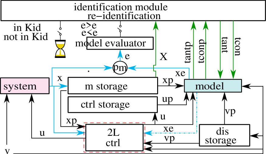
For the fuzzy model of every subsystem (a collection of fuzzy rules with the formulation (V-A) defined for all the state variables of the subsystem), the parameter vectors and including the antecedent and consequent parameters of the fuzzy rules, are (re-)identified at time steps . The most recent element of before the current time step is shown by . Re-identification of at control time step is influenced by the most recent identified vector, , the datasets and , which consist of the elements of vectors and (with the number of reliable measurements of the states and external disturbances received at the sampling times between and ), and dataset , which includes the optimal values of the control input that influences the state of subsystem directly, between time steps and . The elements of can be determined offline using fast multi-parametric optimization approaches [14]:
| (7) | ||||
with a generally nonlinear operator. The updated type-2 fuzzy sets in the antecedents of the fuzzy rules of the subsystem’s model are obtained by
where is a generally nonlinear operator that receives the corresponding parameters and gives the type-2 fuzzy sets of the antecedent. Note that is used for the sake of brevity of the notations and is equivalent to .
The parameter vectors of the fuzzy rules in the model of subsystem can be updated at time step , by minimizing the cumulative error of the state variables estimated by the model within a predefined time window, w.r.t their measured values (see Figure 7). This time window at control time step is denoted by , and includes a predefined number of the most recent elements within . We can write
| (8) |
In (V-C), the fuzzy model (V-A) is re-run within the time window , assuming that the updated at time step is used for all the previous time steps. The optimization problem (V-C) is in general nonlinear, nonsmooth, and nonconvex, and can be solved by standard optimization algorithms, such as pattern search, genetic algorithm, or gradient-based optimization approaches, using multiple starting points.
Figure 7 shows a simplified view of the identification procedure for the consequent parameters of the fuzzy model for subsystem (note that the updated version of the vector of the consequent parameters is indicated by ). More details, including(re-)identification of the antecedent and consequent parameters and the interactions and connections with the proposed two-layer control system, are illustrated in Figure 7.The two-layer control system, receives the time-delayed measurements (indicated by )from the measurement storage and the current measured state (indicated by )from the subsystem in case it is available, or otherwise the estimated value of the current state variable (indicated by ) provided by the fuzzy model, together with the current and the previous corresponding external disturbances (indicated by and ). The control system then produces the control input and injects it to the subsystem and to the control input storage. In Figure 7, the signals illustrated by solid blue arrows correspond to those time steps at which a reliable measurement of the subsystem’s state variable exists. The signal that is shown by the dash-dotted blue arrow realizes otherwise. From this figure, we see that the identification procedure occurs at specific time steps (cf. Remark 6).The signals that are illustrated by solid green arrows will be activated only at these identification time steps.
V-D Parameter tuning for fuzzy-control agents
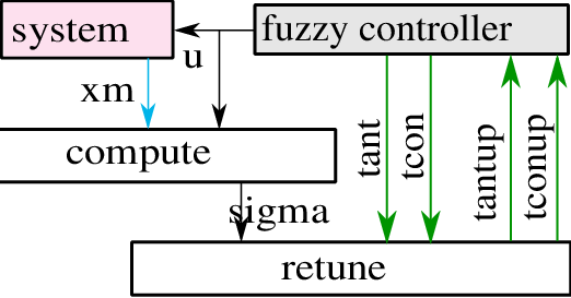
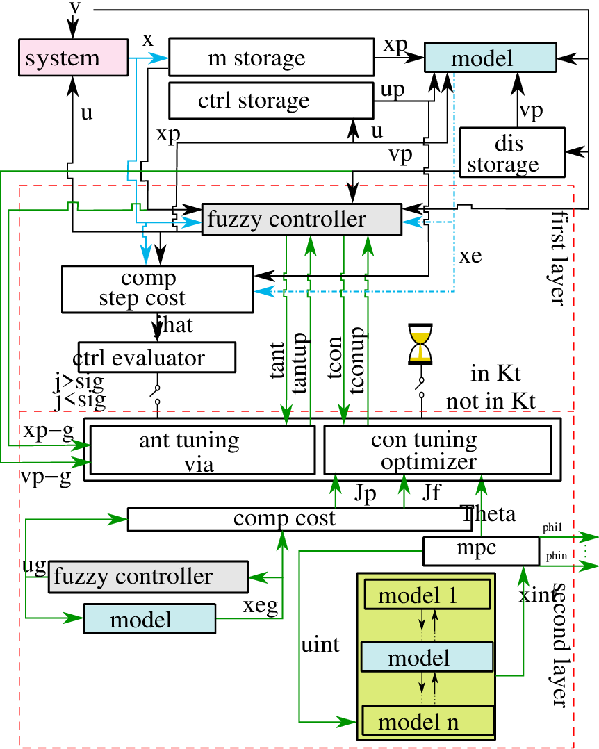
A fuzzy-control agent specified by (V-B), includes two vectors and of design parameters that should be(re-)tuned regularly (at time steps ), to guarantee a satisfactory performance for the control system. The two-layer control architecture (see Figure 5 for an overall view and Figure 9 for extra details) has been designed specifically for efficient performance and tuning of the fuzzy controller (V-B). In order to clarify the links between Figures 5, 7, and 9, the dashed red boxes have been used. The detailed structure shown within the red boxes in Figure 9 includes the main elements of the proposed two-layer control system, which is shown and encountered by similar dashed red boxes in Figures 5 and 7. Next, we elaborate the tuning procedure and Figure 9.
Figure 9 simplifies the tuning procedure, which occurs at the top control layer, while Figure 9 shows the detailed structure of both layers of the proposed integrated control system. From Figure 9, at some regular and triggered control time steps (when the step cost value exceeds a threshold ), the top control layer comes into action. In that case, the signals shown in green in Figures 9 and 9 will be activated. The parameters of the antecedents of the fuzzy control rules for subsystem are updated based on the most recent values of the vector updated at time step , and the datasets and , which include the elements of and (with the number of the reliable measurements of the states and external disturbances available between control time steps and ). Therefore, we have
| (9) |
with a generally nonlinear operator and the most recent element of before control time step . The updated type-2 fuzzy sets in the antecedents of the fuzzy rules of the fuzzy controller are given by
| (10) | ||||
where is a generally nonlinear operator.
The global control objective is to reduce the realized cumulative value of a predefined cost function for all subsystems , , by the end of the control procedure. Correspondingly, in designing the tuning procedure for , reduction of the cumulative cost will be taken into account. Additionally, the mutual interactions of the fuzzy-control agents that may influence the performance and local costs of the dynamically connected subsystems should be considered. Therefore, supposing that the number of control inputs of subsystem is , the MPC module solves the following minimization problem within the time window to tune the consequent parameters of the control fuzzy rules, where is the optimization variable:
| (11) | ||||
with and the weighting factors for, respectively, the past and the future cumulative cost values, an optimal value for the future cumulative local cost of subsystem that is computed by the MPC module (details on the computation of will be given in Section VI), and the prediction horizon of the MPC module. Note that for computation of the past and future cumulative cost values, the fuzzy model and the fuzzy-control agent should be run in a loop (see the top control layer in Figure 9) in order to produce the estimated states and control inputs, assuming that the condition holds. In Figure 9, the past and future values of the cost for subsystem are indicated by and , respectively. The optimization problem (V-D) is in general a nonlinear, nonsmooth, and nonconvex problem, and can be solved by standard optimization algorithms.
Remark 11
The MPC module provides coordination among the distributed fuzzy-control agents by optimizing the global cumulative cost of the entire system and computation of the corresponding optimal values of the local costs for the dynamically connected subsystems.
VI Top layer: MPC module

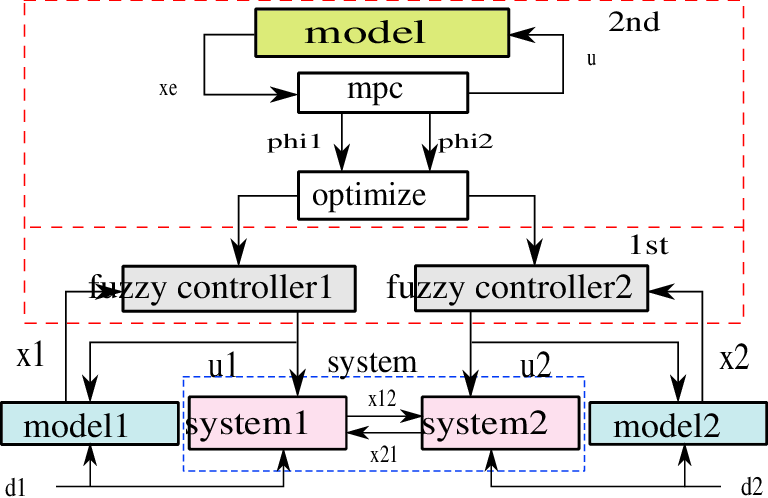
In this section, we explain the performance of the MPC module in more detail. For the sake of simplicity and brevity, we give the formulas for two dynamically connected subsystems 1 and 2 (see Figure 11). We assume that the fuzzy-control agents of the two subsystems have synchronized control time steps. The state and control input vectors of subsystem , , at control time step are denoted by and . The vectors and are the state and control input vectors of the entire system (i.e., and ). Note that to keep the notations simple, in this section we avoid distinguishing the measured and estimated state variables. The external (both to the subsystem and to the entire system) disturbances that affect subsystem at control time step are indicated by . The elements of the state vector of subsystem 1 that directly affect the dynamics of subsystem 2 are kept in a single vector at control time step , which is a subvector of . Subvector of is defined similarly. We have
| (14) | ||||
where and are the total external disturbances for subsystems 1 and 2 at time step and and are the external disturbances (only for the subsystems and not for the entire system) that affect, respectively, subsystem 1 and 2.
Figure 11 shows the block diagram of the proposed two-layer control system applied to these two subsystems. In this case, we consider a prediction horizon of 3 for the MPC module, for the following reasons. The control input of subsystem at control time step , affects the cumulative cost of the entire system both at the current and upcoming control time steps and (see the formulation of in (3)). Moreover, the effect of the control input of subsystem at control time step , is observed on the state of the subsystem at control time step , when (or a subvector of it) will also act as external disturbance for the other subsystem (see (14)). The influence of this disturbance on the state variable of the other subsystem will only be observed at the next control time step, . Since will affect the cumulative cost of the entire system at control time steps , , and , the minimum required size for the MPC prediction horizon is 3.
The centralized optimization problem that should be solved by the MPC module in the top control layer (see Figure 11) to determine the optimal control inputs for both subsystems, such that the global cumulative cost of the entire system is minimized, for a prediction horizon of 3 is formulated by
| (15) | ||||
with the global cumulative cost of the entire system within the MPC prediction window, a vector that includes all vectors within the MPC prediction window, for , and and operators that give the equality and inequality constraints for the control inputs of the subsystems. An integrated fuzzy model (see Figure 11) should be used for the dynamics of the entire system, which implies that for each subsystem at every control time step, the terms and will affect the disturbances and (see (14)) applied to (V-A).
Note that in (V-A), we can define as a convex function. Based on Remark 4, the resulting fuzzy model for each subsystem will be both convex and smooth. Supposing that , , and are also convex and smooth, then the optimization problem of (15) will be a convex optimization problem that can be solved efficiently by gradient-based methods. The MPC module should compute and send the optimal values, , of the local costs to the subsystems (see Figures 9 and 11). The optimization problem (15) has a decomposable structure [15], and in case the size of the problem increases or the centralized solution becomes too complex or costly to determine, it can be solved via the primal decomposition method [16] with and the private and the complicating variables.
VII Case study: Traffic modeling and control
To assess the proposed modeling and control approaches, we next perform a case study for an urban traffic network.
VII-A Setup

The traffic network shown in Figure 12 consists of two intersections, which have been indicated by ‘‘L’’ and ‘‘R’’ in the figure11 1 Note that the modeling and control approaches proposed in this paper are potentially suited for large-scale systems. In the given cased study, however, we have restricted ourselves to only two subsystems in order to provide more insight and an easier representation of the results.. Each link of this urban traffic network consists of two lanes, which in Figure 12 have been indicated by 1L, …, 7L, and 1R, …, 7R. For intersections L, lanes 1L, 2L, 3L, and 7L, and lanes 4L, 5L, 6L, and 7R act as, respectively, the entrance and exit lanes (see the direction of the red arrows in Figure 12). Similarly, lanes 1R, 2R, 3R, and 7R are the entrance lanes for intersection R, while lanes 4R, 5R, 6R, and 7L are the exit lanes for this intersection.
In the rest of the paper, lanes with the indication numbers 1, …, 6 are referred to as “side lanes”, and lanes with the indication number 7, as the “connecting lanes”. Turning (see the black arrows in Figure 12) is allowed for the vehicles at intersections, except for U-turns. Every intersection has four traffic signals, each controlling all the rights-of-way of the entrance lane on which the traffic light stands. The traffic signals at the opposite entrance lanes of an intersection are synchronized and follow the same schedule (i.e., the green and red phases of the northern/southern traffic signals in Figure 12, as well as those of the western and eastern ones coincide). The length of the side and connecting lanes are 150 m and 300 m respectively, the average vehicle length (including the safety distances from the back and front vehicles) is 7.5 m, and the cycle time of the traffic signals for both intersections is 90 s.
VII-B Modeling
The urban traffic network is divided into two subnetworks, called “subnetwork 1” and “subnetwork 2”, colored in, respectively, grey and pink in the figure. Subnetwork 1 consists of intersection L and lanes 1L, …, 7L, and subnetwork 2 includes intersection R and lanes 1R, …, 7R. Three different classes of fuzzy models describing the behavior of traffic, are developed for each subnetwork: “class 1”, including type-1 membership functions, “class 2”, including probabilistic-fuzzy membership functions, and “class 3”, including fuzzy-fuzzy membership functions. These models will be formulated for two state variables, the total number of vehicles per link () and the number of vehicles in the queue on a link (), and will consist of fuzzy rules with a formulation following (V-A).
We assume that the most reliable measurements of the state variables available at control time step from the traffic sensors, correspond to control time step . Each fuzzy rule is described by: “if , then .” For the traffic scenarios we have considered in this case study, the range of variations of the parameters in the given urban traffic network is limited. Hence, the parameters of the fuzzy sets , , and in the antecedents are assumed fixed, and only the parameter vectors of the consequents will be identified and updated.
The control variable of each subnetwork is the green time of the northern and southern traffic signals (indicated by the red dashed curves in Figure 12). These traffic signals are synchronized, and the green time of the other two traffic signals of each intersection (which are also synchronized), is the difference between the cycle time of the intersection and the control input. The flows of the vehicles that enter the urban traffic network via the source lanes (1L, 2L, 3L, 1R, 2R, 3R) are considered as the external inputs. The fuzzy sets and to which the state variables and the external inputs of the urban traffic network belong, will each be defined for the two qualitative terms “low” and “high”. Additionally, the fuzzy set to which the control inputs belong, will be defined for the two qualitative terms “short” and “long”. Next, we explain the three different fuzzy membership functions that are used for the three classes of fuzzy models.
VII-B1 Type-1 triangular membership function
For the fuzzy models in class 1, we consider type-1 triangular membership functions, for two main reasons: in addition to the simplicity and low computation time, Pedrycz [17] shows that triangular membership functions with the half overlap level when used for modeling, can lead to entropy equalization. The type-1 triangular membership functions used for the models within class 1 are shown in Figure 13.

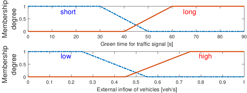
VII-B2 Type-2 probabilistic-fuzzy membership function
The primary and secondary membership functions of the type-2 probabilistic-fuzzy membership functions used in models within class 2, are illustrated in Figure 14. The secondary membership functions in this case are probability functions, which have been considered fixed-value. Each probability function and its corresponding primary membership function have been plotted using the same color. The antecedent of each rule includes three events defined on the state variable , the control input , and the external inputs .
Each status low and high, or short and long, may be interpreted in three different ways (see the blue, red, and black plots in Figure 14). Suppose that , , and indicate the event “ is low” for each of these three interpretations. Similarly, the events “ is high”, “ is short”, “ is long”, “ is low”, and “ is high” for the three interpretations are indicated by, respectively, , , , and , , , and , , , and , , , and , , .
Consider the antecedent of a specific rule that is described by “if is low and is long and is high”; the three events , , and (for ) should occur at the same time, for this specific rule to be fired. The probability of occurrence of these three events simultaneously, and hence, the activation of this specific fuzzy rule is given by
| (19) | ||||
with the probability function. For the sake of simplicity, we assume that the three events are independent, which results in the following simplified expression:
| (20) |
Therefore, the primary membership degree of the combined event is obtained by aggregation of the corresponding primary type-1 membership functions, or equivalently by determining the minimum or multiplication of the primary membership degrees of the events , , and . The probability that this combined membership degree is realized is computed by (20).


VII-B3 Type-2 fuzzy-fuzzy membership function


In order to develop a fuzzy model of the urban traffic network within class 3, we need to describe the status of the network by fuzzy-fuzzy events (see Section III-A). Therefore, in the linguistic description of the corresponding fuzzy rules, we consider a second qualitative term (“slightly” or “very”) for the descriptive terms low and high, and short and long. The mathematical representation of these qualitative terms, i.e., the type-1 primary and secondary membership functions, is illustrated in Figure 15.
For the type-2 probabilistic-fuzzy membership functions, we considered three different interpretations for each of the terms low and high, and short and long (see the black dashed-dotted, red dotted, and blue solid curves in Figure 14). For computing the output of the fuzzy-fuzzy membership functions, the corresponding fuzzy inference engine will make all the possible combinations of the membership degrees obtained from different interpretations for the state variable, the control input, and the external input. Therefore, considering higher numbers of interpretations for the fuzzy terms can result in a dramatic growth in the computational burden. This problem does not arise with probabilistic-fuzzy membership functions. To reduce the computational burden for the fuzzy-fuzzy membership functions and to make the computations feasible, we have therefore considered two interpretations instead of three for each of the terms low and high, and short and long (see the black dashed-dotted and blue solid curves in Figure 15).
Consider the antecedent of a specific rule that is given by “if is very high and is very short and is slightly low”; the three fuzzy-fuzzy events involved in this antecedent are indicated by , , and (for ), respectively, and their primary membership degrees are given by , , and . Similarly, the secondary membership degrees corresponding to each of these primary membership degrees are denoted by , , and . To find the membership degree of the combined fuzzy-fuzzy events for this antecedent, one should consider all the possible combinations of the primary and secondary membership degrees (in this case, 8 combinations are possible).For each combination , the primary and secondary membership degrees of the combined event are computed by
| (21) | |||
| (22) |
In case two combinations have the same primary membership degree, the one with the maximum secondary membership degree is kept, and the rest of the equal primary membership degrees and their corresponding secondary membership degrees will not be considered for computing the output of the fuzzy inference engine (for more details see [18]). The output of the inference engine of the fuzzy rule is computed based on the approach used in [19].
The maximum number of fuzzy rules that can be constructed for a fuzzy model within class 3 in this case is (i.e., 64), i.e., each of the statements in the antecedent of the fuzzy rules regarding the state variable and the external input can have four various descriptions within the set and the statement regarding the control input adopts either of the four descriptions within the set . This implies that the total number of parameters that should be identified for the type-2 fuzzy-fuzzy model is , i.e., 256 parameters (note that each rule has 4 parameters in its consequent that should be identified). Recall that the number of rules in the rule base of the fuzzy models of class 2 was (i.e., 8), i.e., each of the statements in the antecedent of the fuzzy rules about the state variable and the external input could accept either of the two descriptions within the set and the statement about the control input could adopt either of the two descriptions within the set .
As explained before, the computational burden for class 3 of the fuzzy models is very high, and may grow dramatically with the number of fuzzy rules. To reduce the computational burden of both the identification procedure and the computations of the fuzzy inference engine, we have considered 8 rules for class 3 of the fuzzy models, just as for class 2.
VII-B4 Model identification


Now, we explain the procedure of identifying the fuzzy models within class 1, class 2, and class 3. Data collected from the urban traffic network simulated within NetLogo [20], is used to identify and validate the fuzzy models. The urban traffic network illustrated in Figure 12 was simulated in NetLogo, using Gipps’ car following model [21]. The data was collected in a 15 min run of the NetLogo simulator for random time-varying inflows of vehicles at the source lanes (these inflows have been considered such that all sources of the urban traffic network are exposed to low, moderate, and high inflows of vehicles). Data, including the state variables, the control inputs, and the external inputs were collected and saved, where 80% of the collected data was used for identification and the other 20% was used for validation of the fuzzy models. The relative validation errors of the three classes of fuzzy models are shown in Figure 16. Comparing the type-1 and the probabilistic-fuzzy model, we see that the latter has a lower validation relative error in almost all the cases. The fuzzy-fuzzy model is, however, the least accurate one among the three model classes. This can be due to the simplifications (reducing the number of primary membership functions from 3 to 2, and reducing the number of possible rules in the rule base) that had to be made to make the identification tractable, which in itself reveals a limitation for fuzzy-fuzzy membership functions.
Note that the computation times for identifying the type-1 and the probabilistic-fuzzy models were very close to each other, while for the fuzzy-fuzzy model, this computation time was significantly higher. Therefore, the overall conclusion is that class 2 of the fuzzy models, which uses the newly proposed probabilistic-fuzzy membership functions, show clear advantage compared with class 1 and class 3 of models, which use type-1 and fuzzy-fuzzy membership functions.
VII-C Control
In this section, two different control systems will be designed for the urban traffic network shown in Figure 12. The first control system includes a decentralized architecture, while in the second case, a coordinated control system is considered. In either of these two cases, each subnetwork will be controlled by one fuzzy controller that decides about the green time of the northern/southern traffic signal.
The choice of a decentralized architecture for the comparison has two main reasons. First, since the computations are done by similar fuzzy controllers as those in the proposed integrated control architecture, both control systems will have almost similar computation times, which makes the comparison of the performances more fair. Second, with this comparison, we can see how significant the role of the second proposed layer including the MPC tuning module can be.
The fuzzy rules of the fuzzy controllers corresponding to intersections L and R are defined by, respectively:
“if ,
then ”
and
“if ,
then ”,
with , , , and
fuzzy sets, and , , ,
, , and
the tuning parameters.
In the computation of the control inputs, the cumulative states ,
, , and
(i.e., the expected cumulative number of vehicles in the upcoming cycle in the north-south and east-west
directions of intersections L and R) on the influencing lanes are considered:
the green times of the northern and southern traffic signals of subnetworks 1 and 2
are influenced by the number of vehicles on, respectively, the source lanes 2L and 3L, and 2R and 3R
(see Figure 12).
The expected cumulative number of vehicles in the upcoming cycle observed on lanes 2L and 3L, is the summation of the total number of vehicles on these lanes at the current time step and the expected inflow via these source lanes times the cycle time. Moreover, is the summation of the total number of vehicles on lanes 1L and 7L at the current time step and the expected inflow via these source lanes times the cycle time. The cumulative states and are defined in a similar way.
Next, we discuss the two different control systems that have been designed and evaluated for the urban traffic network. In order to evaluate and compare the two cases, four different traffic scenarios within 5-min simulations were considered. Due to the random nature of the simulations (resulting from the inflows of vehicles and the route each vehicle takes in the urban traffic network), each scenario was simulated 10 times for each experiment, and the average total travel time (TTT) of the vehicles in the urban traffic network was computed.
VII-C1 Decentralized fuzzy control


First, we consider a decentralized fuzzy control system for the two intersections in Figure 12 (i.e., one fuzzy controller decides about the green time of the northern/southern traffic signal of each intersection independently, without coordinating with the other fuzzy controller). Each fuzzy controller will be tuned individually. We will consider two cases: fuzzy controllers that implement type-1 triangular membership functions, and fuzzy controllers that use type-2 probabilistic-fuzzy membership functions. Note that in modeling the urban traffic network using fuzzy membership functions (see Section VII-B), type-2 fuzzy-fuzzy membership functions showed to be computationally inefficient or even unfeasible. Hence, we have not considered them for control.
The type-1 triangular and type-2 probabilistic-fuzzy membership functions used for the fuzzy controllers are shown in Figures 18 and 18. Table III shows the results, where the second, third, and fourth columns of this table include the TTT for a decentralized control system for which each fuzzy controller uses type-1 triangular membership functions illustrated in Figure 18, the TTT for a decentralized control system for which each fuzzy controller uses type-2 probabilistic-fuzzy membership functions illustrated in Figure 18, and the relative difference of the TTT.
From Table III, we see that the decentralized fuzzy control system in which each fuzzy controller uses a probabilistic-fuzzy membership function, outperforms the one in which the type-1 triangular membership functions are used by the fuzzy controllers. In general, the difference between the TTT of the vehicles in the urban traffic network for the given four scenarios varies between 100-200 min (which is around 8-15% of the least TTT obtained for each scenario).
| Scenario | TTT [min] for type-1 MF | TTT [min] for probabilistic-fuzzy MF | relative difference of TTT (%) |
| 1 | |||
| 2 | |||
| 3 | |||
| 4 |
| Scenario | TTT [min] for decentralized control | TTT [min] for coordinated control | relative difference of TTT (%) |
| 1 | |||
| 2 | |||
| 3 | |||
| 4 |
VII-C2 Coordinated predictive-fuzzy control
Next, we consider a coordinated control system, which includes an MPC module that takes part in tuning the fuzzy controllers (see Section VI for more details). Since the MPC module considers the entire traffic network as a whole, under a centralized vision, the mutual effects of the dynamics of the two subnetworks on one another will be included in the tuned parameters. Since the results corresponding to the decentralized control system revealed that the probabilistic-fuzzy membership functions outperform the type-1 triangular ones, here only the probabilistic-fuzzy membership functions have been considered for the coordinated controllers.
Table III illustrates the results corresponding to the coordinated control system next to the results obtained for the decentralized control system with probabilistic-fuzzy membership functions given in the previous section. From these results, we see that compared with the decentralized fuzzy control system, the coordinated fuzzy control system gives the least TTT for the vehicles in the urban traffic network for all the given four scenarios. The difference between the realized values of the TTT for these two control systems for the different scenarios varies between 100-700 min (which is around 8-87.5% of the least TTT obtained for each scenario).
VIII Conclusions and Future Research
We have proposed a novel two-layer control architecture that integrates intelligent and model-predictive control. The resulting integrated multi-agent control system is potentially suited for controlling large-scale and complex-dynamics systems in real time. This control architecture has a very low computation time, and provides significant control characteristics, including adaptivity and coordination, and aims at excellent performance. Moreover, a general treatment of type-2 fuzzy sets, and correspondingly type-2 membership functions has been given. This topic has led to the introduction of two different categories of type-2 fuzzy membership functions (probabilistic-fuzzy, which is a fully novel concept that has been proposed in the current paper, and fuzzy-fuzzy), which provide more flexibility and potential in the use of fuzzy sets and fuzzy membership functions.
The proposed modeling and control approaches have been implemented to an urban traffic network. The results of the case study show that in modeling the urban traffic network, the probabilistic-fuzzy membership functions outperform the type-1 triangular and type-2 fuzzy-fuzzy membership functions, considering both the computation time and accuracy. Similarly, probabilistic-fuzzy membership functions provide the best performance in control. Moreover, the proposed integrated architecture has a significantly better performance than a decentralized one that excludes the coordinating MPC module; more specifically, the total travel time can be reduced by up to 87.5% using the proposed control architecture.
Topics for future research include implementation of a distributed MPC module (instead of the current centralized setup with only one MPC controller) in the top control layer, in order to deal with large-scale systems; and in-depth assessment of stability, scalability, and attainable performance improvements of the proposed approach, e.g., via extensive simulations.
Acknowledgment
Research supported by a Niels Stensen Fellowship.
References
- [1] K. P. Sycara, “Multi-agent systems,” AI Magazine, vol. 19, no. 2, pp. 79–92, 1998.
- [2] E. Olivera, K. Fischer, and O. Stepankova, “Multi-agent systems: Which research for which applications,” Robotics and Autonomous Systems, vol. 27, no. 1–2, pp. 91–106, 1999.
- [3] R. R. Negenborn, B. De Schutter, and J. Hellendoorn, “Multi-agent model predictive control for transportation networks: Serial versus parallel schemes,” Engineering Applications of Artificial Intelligence, vol. 21, no. 3, pp. 353–366, 2008.
- [4] R. R. Negenborn, G. Hug-Glanzmann, B. De Schutter, and G. Andersson, “A novel coordination strategy for multi-agent control using overlapping subnetworks with application to power systems,” in Efficient Modeling and Control of Large-Scale Systems (J. Mohammadpour and K. Grigoriadis, eds.), pp. 251–278, USA: Springer, 2010.
- [5] M. Tambe, “Implementing agent teams in dynamic multi-agent environments,” Applied Artificial Intelligence, vol. 12, no. 2–3, pp. 189–210, 1998.
- [6] A. Jamshidnejad, B. De Schutter, and M. Mahjoob, “Urban traffic control using a fuzzy multi-agent system,” in Proceedings of the 2015 European Control Conference, (Linz, Austria), pp. 3046–3051, July 2015.
- [7] F. P. Maturana, R. J. Staron, and K. H. Hall, “Methodologies and tools for intelligent agents in distributed control,” IEEE Intelligent Systems, vol. 20, no. 1, pp. 42–49, 2005.
- [8] C. J. Harris, C. G. Moore, and M. Brown, Intelligent Control: Aspects of Fuzzy Logic and Neural Nets. Singapore: World Scientific, 1994.
- [9] J. Maciejowski, Predictive Control with Constraints. UK: Prentice Hall, 2002.
- [10] L. A. Zadeh, “The concept of a linguistic variable and its application to approximate reasoning,” Information Sciences, vol. 8, no. 3, pp. 199–249, 1975.
- [11] M. Eisen, Introduction to Mathematical Probability Theory. USA: Prentice-Hall, 1969.
- [12] D. Debeljković, Time-Delay Systems. Croatia: InTech, 2011.
- [13] T. Takagi and M. Sugeno, “Fuzzy identification of systems and its applications to modeling and control,” IEEE Transactions on Systems, Man, and Cybernetics, vol. 15, no. 1, pp. 116–132, 1985.
- [14] A. Bemporad, M. Morari, V. Dua, and E. N. Pistikopoulos, “The explicit linear quadratic regulator for constrained systems,” Automatica, vol. 38, no. 1, pp. 3–20, 2002.
- [15] D. P. Palomar and M. Chiang, “A tutorial on decomposition methods for network utility maximization,” IEEE Journal on Selected Areas in Communications, vol. 24, no. 8, pp. 1439–1450, 2006.
- [16] A. Bemporad, M. Heemels, and M. Johansson, Networked Control Systems. Germany: Springer-Verlag, 2010.
- [17] W. Pedrycz, “Why triangular membership functions?,” Fuzzy Sets and Systems, vol. 64, no. 1, pp. 21–30, 1994.
- [18] H. J. Zimmermann, Fuzzy Set Theory – and Its Applications. USA: Kluwer Academic Publishers Norwell, 1996.
- [19] Q. Liang and J. M. Mendel, “An introduction to type-2 TSK fuzzy logic systems,” in Proceedings of the IEEE International Conference on Fuzzy Systems, (South Korea), pp. 1534–1538, 1999.
- [20] U. Wilensky, “Netlogo.” http://ccl.northwestern.edu/netlogo/. Center for Connected Learning and Computer-Based Modeling, Northwestern University, Evanston, IL, 1999. Accessed: 2017-10-30.
- [21] P. G. Gipps, “A behavioural car-following model for computer simulation,” Transportation Research Part B: Methodological, vol. 15, no. 2, pp. 105–111, 1981.