跳到论文正文
W Papers独立论文阅读器 arXiv:1908.10580 论文正文 计算阅读时间 · 0%
引用这篇论文根据当前论文元数据生成,正式投稿前建议核对。


License: arXiv.org perpetual non-exclusive license
arXiv:1908.10580v3 [math.NA] 07 Jul 2020

Analysis of a localised nonlinear Ensemble Kalman Bucy Filter with complete and accurate observations

Jana de Wiljes Thanks: Universität Potsdam, Institut für Mathematik, Karl-Liebknecht-Str. 24/25, D-14476 Potsdam, Germany (wiljes@uni-potsdam.de) and University of Reading, Department of Mathematics and Statistics, Whiteknights, PO Box 220, Reading RG6 6AX, UK    Xin T. Tong Thanks: National University Singapore,10 Lower Kent Ridge Road, Singapore 119076 (mattxin@nus.edu.sg)
Abstract

Concurrent observation technologies have made high-precision real-time data available in large quantities. Data assimilation (DA) is concerned with how to combine this data with physical models to produce accurate predictions. For spatial-temporal models, the Ensemble Kalman Filter with proper localization techniques is considered to be a state-of-the-art DA methodology. This article proposes and investigates a localized Ensemble Kalman Bucy Filter (l-EnKBF) for nonlinear models with short-range interactions. We derive dimension-independent and component-wise error bounds and show the long time path-wise error only has logarithmic dependence on the time range. The theoretical results are verified through some simple numerical tests.

1 Introduction

With the advancement of technology, we now have access to vast amounts of high-precision data in many areas of science. It is important to develop robust and efficient tools to combine the available data with refined large-scale physical models. This study is known as data assimilation (DA) and typically the goal is to produce accurate real-time estimations of the current state of the system.

In geophysical problems, the considered models often have vast spatial scales, therefore millions of state variables are needed to store information at different locations. Such high dimensionality poses a severe challenge to DA methodologies, since the associated computations are expensive and direct global uncertainty quantification tends to be erroneous. Over the last two decades, various computationally feasible approaches have been developed with practical success [28, 14, 7, 25]. One of the most popular algorithms among these is the Ensemble Kalman filter (EnKF). It has been first derived in [7] and heavily advanced and employed in the field of numerical weather prediction. To combat dimensionality issues arising due to the extent of the spatial domain, the so called localization techniques are often employed for the EnKF [27, 9]. The key motivation behind localization is that many systems exhibit a natural decrease in spatial correlation. This can guide artificial tunings of the empirical covariance matrix to avoid spurious correlations.

The empirical success of EnKF has aroused great interest in understanding the underlying theoretical properties [15, 30, 2, 1]. EnKFs can be interpreted as Monte Carlo implementations of the Kalman Filter [13, 12, 8, 23, 17] which is derived for linear prediction and observation models. Therefore most theoretical studies of EnKFs assume a linear setting [22, 4, 6, 21, 29]. Existing analysis of EnKFs for nonlinear models concern mostly the boundedness of algorithm outputs [16, 30, 15], which is not helpful in understanding EnKF performance. The only exception is a recent work [5], where accuracy and stability results have been derived assuming abundant and accurate observations. However, the results there do not consider localization, and hence they require the sample size to be larger than the state dimension. This is infeasible in practice.

This paper intends to close the aforementioned gaps, i.e. nonlinearity and high dimensionality in filter performance analysis, by investigating a localised Ensemble Kalman-Bucy Filter (l-EnKBF). Following [5], we assume abundant and accurate observations are available. Since most geophysical models are formulated through partial differential equations or their discretizations, the associated prediction dynamics often have a short interaction range. This is often paired with a short decorrelation length in the localization technique to reduce the potential spurious long-range correlations. Under these assumptions, we show that l-EnKBF estimation error for each component is bounded independent of the overall dimension, both in the sense of mean square and the moment generating function. Such result does not exist in literature for DA analysis, based on our knowledge. Some related dimension-independent error analysis can be found in [21, 29], but the error estimates are implicit and the models are assumed to be linear. Moreover, we also show the long time path-wise error has a logarithmic dependence on the time range, which is much weaker than the square root dependence in [5]. All these results indicate l-EnKBF has stable and accurate estimation skills.

In Section 2 the underlying setting is outlined and the considered l-EnKBF will be defined. Upper and lower bounds for the empirical second moment are derived in Section 3.1. Then point-wise and path-wise bounds for the mean squared error and a Laplace type condition are derived in Section 3.2 in the l2l_{2} sense, and in Section 3.3 in the component-wise sense. We allocate the proofs of our results in the appendix. In Section 4, the numerical sensitivity of an implementation of the considered l-EnKBF with respect to the underlying assumptions is tested for the Lorenz 96 system.

Throughout the article we assume (∥⋅∥,⟨⋅,⋅⟩)(\|\cdot\|,\langle\cdot,\cdot\rangle) denotes the l2l_{2}-norm with its corresponding inner product. Given a matrix A∈ℝm×nA\in\mathbb{R}^{m\times n} the l2l_{2}-operator norm is defined as

‖A‖=max‖x‖=1⁡‖A​x‖=λmax​(A⊤​A),\|A\|=\max_{\|x\|=1}\|Ax\|=\sqrt{\lambda_{\max}(A^{\top}A)},\\

where λmax\lambda_{\max} denotes the largest eigenvalue of a matrix. The following two matrix norms are also useful to us:

‖A‖1=max⁡∑i=1m1≤j≤n⁡|Ai,j|\displaystyle\|A\|_{1}=\max_{1\leq j\leq n}\sum_{i=1}^{m}|A_{i,j}|
‖A‖max=maxi​j⁡|[A]i,j|\displaystyle\|A\|_{\max}=\max_{ij}|[A]_{i,j}|

where both Ai,jA_{i,j} and [A]i,j[A]_{i,j} denote the entries of the matrix AA. The bracket notation is necessary to denote matrix entries such as [A−1]i,j[A^{-1}]_{i,j} or [A​B]i,j[AB]_{i,j}. Given two symmetric matrices AA and BB then A⪰BA\succeq B implies the matrix A−BA-B is positive semidefinite, which is equivalent to vT​(A−B)​v≥0v^{T}(A-B)v\geq 0 for all v∈ℝnv\in\mathbb{R}^{n}. Given a covariance matrix Γ\Gamma the Mahalanobis norm is defined by ‖v‖Γ2=vT​Γ−1​v\|v\|^{2}_{\Gamma}=v^{T}\Gamma^{-1}v. Lastly, in order to describe the smallness of certain quantities, we use the Big Theta notation. In particular, a quantity aϵa_{\epsilon} is Θ⁡(ϵp)\Theta(\epsilon^{p}), if there is a ϵ\epsilon-independent constant C>0C>0 and c>0c>0 so that c​ϵp≤aϵ≤C​ϵpc\epsilon^{p}\leq a_{\epsilon}\leq C\epsilon^{p}.

2 Problem setup

In this paper, we consider a continuous-time filtering problem, formulated by

d​Xt=f⁡(Xt)​d​t+2​σ​d​Wt,d​Yt=H​Xt​d​t+R​d​Bt.\begin{gathered}dX_{t}=f(X_{t})dt+\sqrt{2}\sigma dW_{t},\\ dY_{t}=HX_{t}dt+RdB_{t}.\end{gathered} (1)

In (1), Xt∈ℝNxX_{t}\in\mathbb{R}^{N_{x}} represents the system we try to recover. We assume its initial distribution is given by X0∼π0X_{0}\sim\pi_{0}. Its dynamics is driven by a deterministic forcing described by a map f:ℝNx→ℝNxf:\mathbb{R}^{N_{x}}\rightarrow\mathbb{R}^{N_{x}} and a stochastic forcing term 2​σ​d​Wt\sqrt{2}\sigma dW_{t}. We assume linear noisy observations Yt∈ℝNyY_{t}\in\mathbb{R}^{N_{y}} of the system are available. In (1), the matrices σ\sigma and RR are positive definite matrices, and Wt∈ℝNxW_{t}\in\mathbb{R}^{N_{x}} and Bt∈ℝNyB_{t}\in\mathbb{R}^{N_{y}} are independent Wiener processes.

In many spatial models, each model component is representing a state information at one spatial location. This introduces a natural distance between two indices, which we will denote as 𝐝\mathbf{d}. As a simple example, For example, if the indices are representing themself on the interval [1,n][1,n], then 𝐝⁡(i,j)\mathbf{d}(i,j) can be taken as |i−j||i-j|. For another example, if the indices are representing equally spaced points on a length nn circle, then 𝐝⁡(i,j)\mathbf{d}(i,j) be taken as min⁡{|i−j|,n−|i−j|}\min\{|i-j|,n-|i-j|\}.

We will use xi​(t)x_{i}(t) to denote the ii-th component of XtX_{t}, so Xt=[x1​(t),…,xNx​(t)]TX_{t}=[x_{1}(t),\ldots,x_{N_{x}}(t)]^{T}. We will also use fif_{i} and wi​(t)w_{i}(t) to denote the ii-th component of ff and WtW_{t}. For notational simplicity, we will often write xi​(t)x_{i}(t) as xix_{i} and wi​(t)w_{i}(t) as wiw_{i}, whenever their dependence on time is evident. Then the SDE that xix_{i} follows is given by

d​xi=fi​(Xt)​d​t+2​σ​d​wi.dx_{i}=f_{i}(X_{t})dt+\sqrt{2}\sigma dw_{i}. (2)

Note that different components are interacting through the drift term, as fi​(Xt)f_{i}(X_{t}) could have dependence on xj​(t)x_{j}(t) for j≠ij\neq i. But in many physical processes, such interactions are of short range, meaning the dependence of fi​(Xt)f_{i}(X_{t}) on xj​(t)x_{j}(t) decays with 𝐝⁡(i,j)\mathbf{d}(i,j). More generally, this can be formulated as

Assumption 2.1 (Short range interaction)

There is a sequence of Lipschitz constants ℱk\mathcal{F}_{k}, such that for any X=[x1,…,xNx]X=[x_{1},\ldots,x_{N_{x}}] and X′=[x1′,…,xNx′]X^{\prime}=[x^{\prime}_{1},\ldots,x^{\prime}_{N_{x}}], the following holds

|fi​(X)−fi​(X′)|≤∑j=1Nxℱ𝐝⁡(i,j)​|xj−xj′|.|f_{i}(X)-f_{i}(X^{\prime})|\leq\sum_{j=1}^{N_{x}}\mathcal{F}_{\mathbf{d}(i,j)}|x_{j}-x^{\prime}_{j}|.

To have a single number controlling the overall stability of the system, we will consider the largest row sum of these Lipschitz constants and define

Cf:=max⁡∑j=1Nxi⁡ℱ𝐝⁡(i,j).C_{f}:=\max_{i}\sum_{j=1}^{N_{x}}\mathcal{F}_{\mathbf{d}(i,j)}. (3)

We will assume that CfC_{f} is a constant independent of the dimension NxN_{x}. This can be verified if ℱk\mathcal{F}_{k} decays to zero exponentially with increasing kk. In Section 4, we demonstrate how to verify Assumption 2.1 on the Lorenz 96 model, assuming all components are bounded.

In computational models, Assumption 2.1 often holds if the spatial resolution is at the same scale of the spatial correlation length. A large NxN_{x} indicates that the spatial domain size is large. It is worthwhile mentioning that, it is also possible to obtain a high dimensional model with a moderate size spatial domain, if one use very small spatial resolution. But Assumption 2.1 is unlikely to hold in such a setting, and localization techniques are not meant to resolve such high dimensionality. One should use dimension reduction techniques instead [21]. The difference between these two high dimensional settings are discussed in [24, 31].

2.1 Localized ensemble Kalman-Bucy filter

Here we will consider a deterministic EnKBF first proposed in [2] that has been shown to be the time limit of a broad class of Ensemble Square Root Filters [18]. Let {Xti}i=1,…,M\{X^{i}_{t}\}_{i=1,\ldots,M} be the ensemble of particles which describe the uncertainty of XtX_{t}. To run the considered algorithm, each of the particle is initialized at a random location from π0\pi_{0} and then driven by the following dynamics

d​Xti=f⁡(Xti)​d​t+σ2​Pt−1​(Xti−X¯t)​d​t−12​Pt​HT​(R​RT)−1​(H​Xti​d​t+H​X¯t​d​t−2​d​Y​(t)).dX^{i}_{t}=f(X^{i}_{t})dt+\sigma^{2}P^{-1}_{t}(X_{t}^{i}-\overline{X}_{t})dt-\frac{1}{2}P_{t}H^{T}(RR^{T})^{-1}(HX^{i}_{t}dt+H\overline{X}_{t}dt-2dY(t)). (4)

In (4), the sample mean and covariance are defined by

X¯t=1M​∑i=1MXti,Pt=1M−1​∑i=1M(Xti−X¯t)​(Xti−X¯t)T.\overline{X}_{t}=\frac{1}{M}\sum_{i=1}^{M}X^{i}_{t},\quad P_{t}=\frac{1}{M-1}\sum_{i=1}^{M}(X^{i}_{t}-\overline{X}_{t})(X^{i}_{t}-\overline{X}_{t})^{T}.

The posterior distribution of XtX_{t} conditioned on Ys≤tY_{s\leq t} is then approximated by the Gaussian distribution 𝒩⁡(X¯t,Pt)\mathcal{N}(\overline{X}_{t},P_{t}). It is important to mention that for a linear drift ff the EnKBF in (4) converges to the KBF for M→∞M\rightarrow\infty. Further a mean-field limit has been derived for the nonlinear drift scenario [5]. Note that mean field limits of EnKFs for a nonlinear setting have also been derived in [19].

When the dimension is high, EnKBF is in general ill-defined and it can perform poorly. This is because of two reasons. First, the rank of PtP_{t} is at maximum M−1M-1. So if M≪NxM\ll N_{x}, PtP_{t} is singular and its numerical approximated inverse is usually unstable. Second, by random matrix theory, it is known that if XtiX^{i}_{t} are i.i.d. samples from a Gaussian distribution 𝒩⁡(0,P)\mathcal{N}(0,P), in order for the covariance sampler error in l2l_{2}-norm ‖P−Pt‖\|P-P_{t}\| to be small, one needs M=O⁡(Nx)M=O(N_{x}). In other words, PtP_{t} is a very inaccurate approximation of the true posterior covariance when M≪NxM\ll N_{x} [29].

In practice, one popular way to resolve the issues mentioned above is to apply covariance localization. Mathematically, this operation can be formulated as replacing PtP_{t} in (4) with PtL=Pt∘ϕP^{L}_{t}=P_{t}\circ\phi. Here ∘\circ denotes the component-wise product or Schur product, so the components of PtLP_{t}^{L} are defined as

[PtL]i,j:=[Pt]i,j​ϕi,j.[P^{L}_{t}]_{i,j}:=[P_{t}]_{i,j}\phi_{i,j}. (5)

The symmetric matrix ϕ\phi here is called a localization matrix. Its components are nonnegative. They are of value 11 at the diagonal, and decay to zero extremely fast along the off diagonal direction. One popular choice takes the form of ϕi,j=ρ⁡(𝐝⁡(i,j)l)\phi_{i,j}=\rho(\frac{\mathbf{d}(i,j)}{l}), where ρ\rho is a function from (4.10) in [9]

ρ⁡(x)={−14x5+12x4+58x3−53x2+1,|x|≤1;112x5−12x4+58x3+53x2−5x+4−23​x,1≤|x|≤2;02≤|x|.\rho(x)=\begin{cases}-\frac{1}{4}x^{5}+\frac{1}{2}x^{4}+\frac{5}{8}x^{3}-\frac{5}{3}x^{2}+1,\quad&|x|\leq 1;\\ \frac{1}{12}x^{5}-\frac{1}{2}x^{4}+\frac{5}{8}x^{3}+\frac{5}{3}x^{2}-5x+4-\frac{2}{3x},\quad&1\leq|x|\leq 2;\\ 0\quad&2\leq|x|.\end{cases} (6)

where ll denotes the typical decorrelation length, which we assume to be independent of NxN_{x}. We will consider again the largest row sum of ϕ\phi, and define

Cϕ:=max⁡∑j=1Nxi⁡ϕi,j.C_{\phi}:=\max_{i}\sum_{j=1}^{N_{x}}\phi_{i,j}. (7)

We will assume CϕC_{\phi} is a constant independent of the dimension NxN_{x}. This is true for most practical localization matrices including (6).

When the true covariance matrix is spatially localized, PtLP^{L}_{t} is a much better covariance estimator, because the localization operation eliminates spurious long distance correlation errors [3]. Moreover, the localization operation improves the rank, so PtLP^{L}_{t} is often full rank and invertible. But this is not guaranteed in general. So for the rigorousness of this exposition, we use the following inversion

Definition 2.2

If all diagonal entries of PtP_{t} are nonzero, then its diagonal inverse (DI) is given by

[Pt†]i,i=[Pt]i,i−1,[Pt†]i,j=0,∀i,j=1,…,n,i≠j.[P_{t}^{\dagger}]_{i,i}=[P_{t}]_{i,i}^{-1},\quad[P_{t}^{\dagger}]_{i,j}=0,\quad\forall i,j=1,\ldots,n,\,\,i\neq j.

Note that it satisfies the following for all i=1,…,ni=1,\ldots,n

[Pt†​Pt]i,i=[Pt†​Pt]i,i=1.[P_{t}^{\dagger}P_{t}]_{i,i}=[P_{t}^{\dagger}P_{t}]_{i,i}=1. (8)

In the original EnKBF formulation (4), we replace PtP_{t} with PtLP_{t}^{L} and Pt−1P_{t}^{-1} with Pt†P_{t}^{\dagger} and we obtain the localized EnKBF (l-EnKBF):

d​Xti=f⁡(Xti)​d​t+σ2​Pt†​(Xti−X¯t)​d​t−12​PtL​HT​(R​RT)−1​(H​Xti​d​t+H​X¯t​d​t−2​d​Yt).dX^{i}_{t}=f(X^{i}_{t})dt+\sigma^{2}P^{\dagger}_{t}(X_{t}^{i}-\overline{X}_{t})dt-\frac{1}{2}P^{L}_{t}H^{T}(RR^{T})^{-1}(HX^{i}_{t}dt+H\overline{X}_{t}dt-2dY_{t}). (9)

As a remark, the using of Pt†P_{t}^{\dagger} simplifies the theoretical derivation in below, since we can verify that Pt†P_{t}^{\dagger} is well defined (see Lemma 3.2 below). Meanwhile, it is an open question on how to generalize our results to other versions of pseudo inverse for PtP_{t}.

2.2 Abundant and accurate observations

When the observation sources are abundant, HH in (1) can be assumed to be of rank NxN_{x}, and there is an H−∈ℝNx×NyH^{-}\in\mathbb{R}^{N_{x}\times N_{y}} such that H−​H=INxH^{-}H=I_{N_{x}}. We can consider the following transformation

X~t=σ−1​Xt,f~​(X)=σ−1​f​(σ​X),Y~t=σ−1​H−​Yt,R~=σ−1​H−​R,\widetilde{X}_{t}=\sigma^{-1}X_{t},\quad\tilde{f}(X)=\sigma^{-1}f(\sigma X),\quad\widetilde{Y}_{t}=\sigma^{-1}H^{-}Y_{t},\quad\widetilde{R}=\sigma^{-1}H^{-}R,

then X~t\widetilde{X}_{t} and Y~t\widetilde{Y}_{t} follow the SDE in below

d​X~t=σ−1​d​Xt=f~​(X~t)​d​t+2​d​Wt,d​Y~t=σ−1​H−​d​Yt=σ−1​Xt+σ−1​H−​R​d​Bt=X~t​d​t+R~​d​Bt.\begin{gathered}d\widetilde{X}_{t}=\sigma^{-1}dX_{t}=\tilde{f}(\widetilde{X}_{t})dt+\sqrt{2}dW_{t},\\ d\widetilde{Y}_{t}=\sigma^{-1}H^{-}dY_{t}=\sigma^{-1}X_{t}+\sigma^{-1}H^{-}RdB_{t}=\widetilde{X}_{t}dt+\widetilde{R}dB_{t}.\end{gathered} (10)

If we apply l-EnKBF (9) to the transformed system (X~t,Y~t)(\widetilde{X}_{t},\widetilde{Y}_{t}), then the sample mean and covariance matrices will follow

x~¯t=σ−1​X¯t,P~t=σ−2​Pt,P~tL=σ−2​PtL,\overline{\tilde{x}}_{t}=\sigma^{-1}\overline{X}_{t},\quad\widetilde{P}_{t}=\sigma^{-2}P_{t},\quad\widetilde{P}^{L}_{t}=\sigma^{-2}P^{L}_{t},

while P~t†\widetilde{P}^{\dagger}_{t} can be taken as σ2​Pt†\sigma^{2}P^{\dagger}_{t}. Then the dynamics of each l-EnKBF particle will satisfy

d​X~ti\displaystyle d\widetilde{X}^{i}_{t} =f~​(X~ti)​d​t+P~t†​(X~ti−x~¯t)​d​t−12​P~tL​(R~​R~T)−1​(X~ti​d​t+x~¯t​d​t−2​d​Y~t)\displaystyle=\widetilde{f}(\widetilde{X}^{i}_{t})dt+\widetilde{P}^{\dagger}_{t}(\widetilde{X}_{t}^{i}-\overline{\tilde{x}}_{t})dt-\frac{1}{2}\widetilde{P}^{L}_{t}(\widetilde{R}\widetilde{R}^{T})^{-1}(\widetilde{X}^{i}_{t}dt+\overline{\tilde{x}}_{t}dt-2d\widetilde{Y}_{t})
=σ−1​f​(Xti)​d​t+σ​Pt†​(Xti−X¯t)​d​t−12​σ−1​PtL​HT​(R​RT)−1​(H​Xti​d​t+H​X¯t​d​t−2​d​Yt)=σ−1​d​Xti.\displaystyle=\sigma^{-1}f(X^{i}_{t})dt+\sigma P^{\dagger}_{t}(X_{t}^{i}-\overline{X}_{t})dt-\frac{1}{2}\sigma^{-1}P^{L}_{t}H^{T}(RR^{T})^{-1}(HX^{i}_{t}dt+H\overline{X}_{t}dt-2dY_{t})=\sigma^{-1}dX^{i}_{t}.

It is evident that the theoretical properties of XtiX^{i}_{t} will be the same as the ones of X~ti\widetilde{X}^{i}_{t}.

Note that (10) corresponds to the original model (1) with σ=1\sigma=1 and H=IH=I. This is a much simplified parameter setting for followup discussion. And from the above derivation, there is no sacrifice of generality by focusing on it. Under this setting, the l-EnKBF formula will be simplified as

d​Xti=f⁡(Xti)​d​t+Pt†​(Xti−X¯t)​d​t−12​PtL​ΩR​(Xti​d​t+X¯t​d​t−2​d​Yt),ΩR:=(R​RT)−1.dX^{i}_{t}=f(X^{i}_{t})dt+P^{\dagger}_{t}(X_{t}^{i}-\overline{X}_{t})dt-\frac{1}{2}P^{L}_{t}\Omega_{R}(X^{i}_{t}dt+\overline{X}_{t}dt-2dY_{t}),\quad\Omega_{R}:=(RR^{T})^{-1}.

When the observations are accurate and independent, the observation noise covariance R​RTRR^{T} is a diagonal matrix with small components. We will use ϵ\epsilon to describe their order. In summary, we have made the following assumption

Assumption 2.3

Through a linear transformation, we assume (1) is transformed to

d​Xt=f⁡(Xt)​d​t+2​d​Wt,d​Yt=Xt​d​t+R​d​Bt\begin{gathered}dX_{t}=f(X_{t})dt+\sqrt{2}dW_{t},\\ dY_{t}=X_{t}dt+RdB_{t}\end{gathered}

Moreover we assume for an ϵ>0\epsilon>0 that Ω=ϵ​(R​RT)−1\Omega=\epsilon(RR^{T})^{-1} is diagonal, and bounded by constants ωmin​I⪯Ω⪯ωmax​I\omega_{\min}I\preceq\Omega\preceq\omega_{\max}I.

Note that Assumption 2.3 implies that R​RT=Θ⁡(ϵ)RR^{T}=\Theta(\epsilon). In other words we assume that the squared observation error covariance matrix is of order ϵ\epsilon.

By replacing ΩR\Omega_{R} with ϵ−1​Ω\epsilon^{-1}\Omega, the l-EnKBF formula is written as

d​Xti=f⁡(Xti)​d​t+Pt†​(Xti−X¯t)​d​t−12​ϵ​PtL​Ω​(Xti​d​t+X¯t​d​t−2​d​Yt).dX^{i}_{t}=f(X^{i}_{t})dt+P^{\dagger}_{t}(X_{t}^{i}-\overline{X}_{t})dt-\frac{1}{2\epsilon}P^{L}_{t}\Omega(X^{i}_{t}dt+\overline{X}_{t}dt-2dY_{t}). (11)

Since X¯t=1M​∑i=1MXti\overline{X}_{t}=\frac{1}{M}\sum_{i=1}^{M}X^{i}_{t}, the sample mean process follows the following dynamics

d​X¯t=f¯t​d​t−ϵ−1​PtL​Ω​(X¯t​d​t−d​Yt),f¯t:=1M​∑i=1Mf⁡(Xti).d\overline{X}_{t}=\overline{f}_{t}dt-\epsilon^{-1}P^{L}_{t}\Omega(\overline{X}_{t}dt-dY_{t}),\quad\overline{f}_{t}:=\frac{1}{M}\sum_{i=1}^{M}f(X^{i}_{t}). (12)

So if we denote Δ​Xti=Xti−X¯t\Delta X^{i}_{t}=X^{i}_{t}-\overline{X}_{t}, it follows the ordinary differential equation (ODE)

dd​t​Δ​Xti=f⁡(Xti)−f¯t+Pt†​Δ​Xti−12​ϵ​PtL​Ω​Δ​Xti.\frac{d}{dt}\Delta X^{i}_{t}=f(X^{i}_{t})-\overline{f}_{t}+P^{\dagger}_{t}\Delta X^{i}_{t}-\frac{1}{2\epsilon}P^{L}_{t}\Omega\Delta X^{i}_{t}.

Because the sample covariance Pt=1M−1​∑i=1MΔ​Xti​(Δ​Xti)TP_{t}=\frac{1}{M-1}\sum_{i=1}^{M}\Delta X^{i}_{t}(\Delta X^{i}_{t})^{T}, we have

dd​t​Pt=(Ft+FtT)+(Pt†​Pt+Pt​Pt†)−12​ϵ​(PtL​Ω​Pt+Pt​Ω​PtL)\frac{d}{dt}P_{t}=(F_{t}+F_{t}^{T})+(P_{t}^{\dagger}P_{t}+P_{t}P_{t}^{\dagger})-\frac{1}{2\epsilon}(P^{L}_{t}\Omega P_{t}+P_{t}\Omega P^{L}_{t}) (13)

where Ft:=1M−1​∑(Xti−X¯t)​(f⁡(Xti)−f¯t)TF_{t}:=\frac{1}{M-1}\sum(X^{i}_{t}-\overline{X}_{t})(f(X^{i}_{t})-\overline{f}_{t})^{T}.

3 Main results

We present our main theoretical results for the l-EnKBF in (9) in this section. To keep to discussion concise, we allocate the technical verifications to the appendix.

3.1 Wellposedness and Stability

Before the accuracy of the filter can be addressed it is crucial to check if the l-EnKBF can blow-up or collapse. In other words, we will demonstrate that the filter is stable, such that there are upper and lower bounds for PtP_{t}. The upper bound is established by the following:

Lemma 3.1

Under Assumptions 2.1 and 2.3, suppose PtLP_{t}^{L} evolving in time according to (13) exists, the following holds

‖Pt‖max≤λmax:=2​ϵωmin​(Cf2+3​ωminϵ),∀t>t∗′:=ωmin​ϵλmax.\|P_{t}\|_{\max}\leq\lambda_{\max}:=\frac{2\epsilon}{\omega_{\min}}\left(\sqrt{C_{f}^{2}+\frac{3\omega_{\min}}{\epsilon}}\right),\quad\forall t>t^{\prime}_{*}:=\frac{\omega_{\min}\epsilon}{\lambda_{\max}}.

And for all t>0t>0, ‖Pt‖max≤max⁡{‖P0‖max,λmax}\|P_{t}\|_{\max}\leq\max\{\|P_{0}\|_{\max},\lambda_{\max}\}. It is clear that when CfC_{f} and ωmin\omega_{\min} are constants, λmax​(ϵ)=Θ⁡(ϵ),t∗′=Θ⁡(ϵ)\lambda_{\max}(\epsilon)=\Theta(\sqrt{\epsilon}),t^{\prime}_{*}=\Theta(\sqrt{\epsilon}).

In [5] the bound depends explicitly on MM (as the Frobenius norm is used to derive the bound). Here a different route is taken which results in a bound independent of MM.

To ensure that the filter does not collapse, it is crucial to have a lower bound on the covariance. This comes as a reverse of Lemma 3.1. For this purpose, we denote

‖Pt‖min=min⁡{[Pt]i,i,i=1,…,Nx}.\|P_{t}\|_{\min}=\min\{[P_{t}]_{i,i},i=1,\ldots,N_{x}\}.

It should be noted that ‖Pt‖min\|P_{t}\|_{\min} is not a norm, and we choose this notation just for its symmetry with ‖Pt‖max\|P_{t}\|_{\max}.

Lemma 3.2

Under Assumptions 2.1 and 2.3, suppose PtLP_{t}^{L} evolves in time according to (13), the following holds for sufficiently small ϵ>0\epsilon>0

‖Pt‖min≥λmin:=ϵ3​λmax​ωmax​Cϕ,∀t>t∗:=ωmin​ϵλmax+3​λmin.\|P_{t}\|_{\min}\geq\lambda_{\min}:=\frac{\epsilon}{3\lambda_{\max}\omega_{\max}C_{\phi}},\quad\forall t>t_{*}:=\frac{\omega_{\min}\epsilon}{\lambda_{\max}}+3\lambda_{\min}.
‖Pt‖min≥min⁡{‖P0‖min,ϵ2​ωmin​max⁡{‖P0‖max,λmax}}>0,∀t>0.\|P_{t}\|_{\min}\geq\min\left\{\|P_{0}\|_{\min},\frac{\epsilon}{2\omega_{\min}\max\{\|P_{0}\|_{\max},\lambda_{\max}\}}\right\}>0,\quad\forall t>0.

It is clear that when CfC_{f} and ωmin\omega_{\min} are constants, λmin​(ϵ)=Θ⁡(ϵ),t∗=Θ⁡(ϵ)\lambda_{\min}(\epsilon)=\Theta(\sqrt{\epsilon}),t_{*}=\Theta(\sqrt{\epsilon}).

Since Pt†P_{t}^{\dagger} is well defined as long as ‖Pt‖min>0\|P_{t}\|_{\min}>0, using the same proof as in Theorem 2.3 of [5], we can show that the l-EnKBF given by (9) has a strong solution:

Corollary 3.3

Suppose the initial ensemble is selected so that ‖P0‖min>0\|P_{0}\|_{\min}>0. Then the l-EnKBF filter is well defined for all t>0t>0.

3.2 Error analysis in l2l_{2} norm

As the next step we consider the accuracy of l-EnKBF in terms of the l2l_{2} norm. Since the filter estimate with the ensemble mean, the error is its deviation from the truth, et=Xt−X¯te_{t}=X_{t}-\overline{X}_{t}. While it has already been shown in [5] ‖et‖2\|e_{t}\|^{2} is of order Nx​ϵN_{x}\sqrt{\epsilon} through tail probability, our new result extends this estimate to the Laplace transforms. Moreover we show the path-wise maximum has the logarithm scaling with time, indicating the filter is highly stable in terms of error.

Theorem 3.4

Let et=Xt−X¯te_{t}=X_{t}-\overline{X}_{t} be the filter error of l-EnKBF (11). Under Assumptions 2.1 and 2.3, if ϕ~:=ϕ−ρ​I⪰𝟎\tilde{\phi}:=\phi-\rho I\succeq\mathbf{0} for a constant ρ>0\rho>0, then for any fixed t0>0t_{0}>0 there are strictly positive constants ϵ0,c\epsilon_{0},c and CC such that for every ϵ∈(0,ϵ0)\epsilon\in(0,\epsilon_{0}),

  1. 1)

    When t>t0,𝔼​‖et‖2≤C​ϵ​Nxt>t_{0},\mathbb{E}\|e_{t}\|^{2}\leq C\sqrt{\epsilon}N_{x}.

  2. 2)

    For any 0<λ<cϵ−1/20<\lambda<c\epsilon^{-1/2},

    lim supt→∞𝔼​exp⁡(λ​‖et‖2)≤2​exp⁡(4​C​λ​Nx​ϵ).\limsup_{t\to\infty}\mathbb{E}\exp(\lambda\|e_{t}\|^{2})\leq 2\exp(4C\lambda N_{x}\sqrt{\epsilon}).
  3. 3)

    For any T>t0T>t_{0}, the following holds

    𝔼t0​[supt0≤t≤T‖et‖2]≤‖et0‖2+C​ϵ​Nx+C​ϵ​log⁡(C​T/ϵ)\mathbb{E}_{t_{0}}\left[\sup_{t_{0}\leq t\leq T}\|e_{t}\|^{2}\right]\leq\|e_{t_{0}}\|^{2}+C\sqrt{\epsilon}N_{x}+C\sqrt{\epsilon}\log(CT/\sqrt{\epsilon})

    Here 𝔼t0\mathbb{E}_{t_{0}} denotes conditional expectation with respect to information available at time t0t_{0}.

Note that the ϵ1/2\epsilon^{1/2} scaling is sharp. This can be understood best if one applies the Kalman-Bucy filter to (1) with f⁡(X)=𝟎f(X)=\mathbf{0}, H=INxH=I_{N_{x}} and R=ϵ​INxR=\sqrt{\epsilon}I_{N_{x}}, the posterior covariance PtP_{t} follows the ODE dd​t​Pt=2​INx−ϵ−1​Pt2\frac{d}{dt}P_{t}=2I_{N_{x}}-\epsilon^{-1}P_{t}^{2}. It is easy to show that PtP_{t} will converge to the limit P∞=2​ϵ​INxP_{\infty}=\sqrt{2\epsilon}I_{N_{x}}, which is of order ϵ1/2\epsilon^{1/2} as well.

3.3 Analysis for component-wise error

While Theorem 3.4 provides an estimate ‖et‖2\|e_{t}\|^{2}, the estimate has a scaling of NxN_{x} because ‖et‖2\|e_{t}\|^{2} is the sum of NxN_{x} component errors. From Theorem 3.4, it is impossible to indicate the error of one specific component, or whether this component’s error is independent of the dimension NxN_{x}. This section shows that with a stronger structure assumption on the localization matrix, we can derive dimension-independent bounds for each individual component.

Assumption 3.5

The localization matrix ϕ\phi is diagonally dominant. In other words, there is a q<1q<1 such that

∑j≠iϕi,j≤q.\sum_{j\neq i}\phi_{i,j}\leq q.

Moreover, the interaction between components can be dominated by a constant CℱC_{\mathcal{F}}-multiple of the matrix structure ϕ\phi:

ℱ𝐝⁡(i,j)≤Cℱ​ϕi,j∀i,j.\mathcal{F}_{\mathbf{d}(i,j)}\leq C_{\mathcal{F}}\phi_{i,j}\quad\forall i,j.

Since ℱd\mathcal{F}_{d} usually decays to zero quickly in practice, so CℱC_{\mathcal{F}} are likely to be found. Using Lemma A.1 it is easy to show ϕ\phi satisfying Assumption 3.5 will have ϕ⪰(1−q)​I\phi\succeq(1-q)I, meaning ϕ~=ϕ−q​I\tilde{\phi}=\phi-qI is positive semidefinite. In other words, Assumption 3.5 is stronger than assumption for ϕ\phi imposed in Theorem 3.4. In general, ϕ\phi is not always diagonally domain. However, this can hold if one choose small localization length ll. For example, for the Gaspari–Cohn [9] distance matrix ϕ\phi, it will be diagonally dominant if l≤1.4l\leq 1.4. In other words, Assumption 3.5 is likely to hold if the components of model represent spatial information of distant apart.

With Assumption 3.5, we can reproduce Theorem 3.4 type of result for individual component.

Theorem 3.6

Let et=Xt−X¯te_{t}=X_{t}-\overline{X}_{t} be the filter error of l-EnKBF (11). Under Assumptions 2.1, 2.3, and 3.5, for any fixed t0>0t_{0}>0 there are constants cc and CC such that for sufficiently small ϵ>0\epsilon>0,

  1. 1)

    When t>t0t>t_{0}, for any index ii, 𝔼⁡[[et]i2]≤C​ϵ\mathbb{E}[[e_{t}]_{i}^{2}]\leq C\sqrt{\epsilon}.

  2. 2)

    For any 0<λ<cϵ−1/20<\lambda<c\epsilon^{-1/2} and index ii,

    lim supt→∞𝔼​exp⁡(λ​[et]i2)≤2​exp⁡(4​C​λ​ϵ).\limsup_{t\to\infty}\mathbb{E}\exp(\lambda[e_{t}]_{i}^{2})\leq 2\exp(4C\lambda\sqrt{\epsilon}).
  3. 3)

    For any T>t0T>t_{0}, the following holds for all ii

    𝔼t0​[supt0≤t≤T[et]i2]≤maxi⁡{[et0]i2}+C​ϵ​log⁡(T/ϵ).\mathbb{E}_{t_{0}}\left[\sup_{t_{0}\leq t\leq T}[e_{t}]^{2}_{i}\right]\leq\max_{i}\{[e_{t_{0}}]^{2}_{i}\}+C\sqrt{\epsilon}\log(T/\sqrt{\epsilon}).

    Here 𝔼t0\mathbb{E}_{t_{0}} denotes conditional expectation with respect to information available at time t0t_{0}.

  4. 4)

    For any T>t0T>t_{0},

    𝔼t0​[max⁡supt0≤t≤Ti⁡[et]i2]≤maxi⁡{[et0]i2}+C​ϵ​log⁡(Nx​T/ϵ).\mathbb{E}_{t_{0}}\left[\max_{i}\sup_{t_{0}\leq t\leq T}[e_{t}]^{2}_{i}\right]\leq\max_{i}\{[e_{t_{0}}]^{2}_{i}\}+C\sqrt{\epsilon}\log(N_{x}T/\sqrt{\epsilon}).

If Z1,…,ZnZ_{1},\ldots,Z_{n} are i.i.d. samples of a Gaussian distribution, a rough estimate of maxi⁡{Zi}\max_{i}\{Z_{i}\} is of order log⁡n\log n. And when system has short range interaction, its components are tend to be independent when they are far apart. Likewise, when a system is stationary, it is close to independent with it self in a distance past. The filter error process happens to have both of these two properties. That is why we have the scaling of log⁡(Nx​T)\log(N_{x}T) in claim 4).

4 Numerical investigation

Lastly the theoretical findings are numerically verified by means of the stochastically perturbed Lorenz 96 system (L96) [20]. The evolution of each spatial component is given by

d​xs​(t)=fs​(X⁡(t))​d​t+2​d​Ws​(t)dx_{s}(t)=f_{s}(X(t))dt+\sqrt{2}dW_{s}(t)

for s∈{1,…,Nx}s\in\{1,\dots,N_{x}\}. Here

fs​(X⁡(t))=(xs+1​(t)−xs−2​(t))​xs−1​(t)−xs​(t)+8,f_{s}(X(t))=\Big({x}_{s+1}(t)-{x}_{s-2}(t)\Big){x}_{s-1}(t)-{x}_{s}(t)+8, (14)

and spatial periodicity is assumed, i.e., x−1​(t)=xNx−1​(t)x_{-1}(t)=x_{N_{x}-1}(t), x0​(t)=xN​(t)x_{0}(t)=x_{N}(t) and xNx+1​(t)=x1​(t)x_{N_{x}+1}(t)=x_{1}(t). Numerically generated trajectories of (14) are typically bounded in the l∞l_{\infty} norm, i.e.,

|xs​(t)|≤C=40|x_{s}(t)|\leq C=40 (15)

for all ss for the Lorenz 96 system. In other words, the solution of (14) is largely indifferent from a soft-truncated version d​Xs​(t)=f^s​(X⁡(t))​d​t+2​d​Ws​(t)dX_{s}(t)=\hat{f}_{s}(X(t))dt+\sqrt{2}dW_{s}(t), where

f~​(xs​(t))=1‖X⁡(t)‖∞≤C​(xs+1​(t)−xs−2​(t))​xs−1​(t)−xs​(t).\tilde{f}(x_{s}(t))=1_{\|X(t)\|_{\infty}\leq C}\Big({x}_{s+1}(t)-{x}_{s-2}(t)\Big){x}_{s-1}(t)-{x}_{s}(t). (16)

Then note that when ‖X⁡(t)‖∞≥C\|X(t)\|_{\infty}\geq C, |f~s​(X⁡(t))−f~s​(X′​(t))|=|xs′​(t)−xs​(t)||\tilde{f}_{s}(X(t))-\tilde{f}_{s}(X^{\prime}(t))|=|{x}^{\prime}_{s}(t)-{x}_{s}(t)|; when ‖X⁡(t)‖∞≤C\|X(t)\|_{\infty}\leq C,

|f~s​(X⁡(t))−f~s​(X′​(t))|\displaystyle|\tilde{f}_{s}(X(t))-\tilde{f}_{s}(X^{\prime}(t))| =|(xs+1​(t)−xs−2​(t))​xs−1​(t)−xs​(t)−[(xs+1′​(t)−xs−2′​(t))​xs−1′​(t)−xs′​(t)]|\displaystyle=|\Big({x}_{s+1}(t)-{x}_{s-2}(t)\Big){x}_{s-1}(t)-{x}_{s}(t)-[\Big({x}^{\prime}_{s+1}(t)-{x}^{\prime}_{s-2}(t)\Big){x}^{\prime}_{s-1}(t)-{x}^{\prime}_{s}(t)]|
≤|(xs+1​(t)−xs+1′​(t))​xs−1​(t)|+|(xs−1​(t)−xs−1′​(t))​xs+1′​(t)|\displaystyle\leq|({x}_{s+1}(t)-{x}^{\prime}_{s+1}(t)){x}_{s-1}(t)|+|({x}_{s-1}(t)-{x}^{\prime}_{s-1}(t)){x}^{\prime}_{s+1}(t)|
+|(xs−2′​(t)−xs−2​(t))​xs−1′​(t)|+|(xs−1′​(t)−xs−1​(t))​xs−2​(t)|+|xs′​(t)−xs​(t)|\displaystyle+|({x}^{\prime}_{s-2}(t)-{x}_{s-2}(t)){x}^{\prime}_{s-1}(t)|+|({x}^{\prime}_{s-1}(t)-{x}_{s-1}(t)){x}_{s-2}(t)|+|{x}^{\prime}_{s}(t)-{x}_{s}(t)|
≤C​|xs+1​(t)−xs+1′​(t)|+C​|xs−1​(t)−xs−1′​(t)|+C​|xs−2′​(t)−xs−2​(t)|\displaystyle\leq C|{x}_{s+1}(t)-{x}^{\prime}_{s+1}(t)|+C|{x}_{s-1}(t)-{x}^{\prime}_{s-1}(t)|+C|{x}^{\prime}_{s-2}(t)-{x}_{s-2}(t)|
+C​|xs−1′​(t)−xs−1​(t)|+|xs′​(t)−xs​(t)|.\displaystyle+C|{x}^{\prime}_{s-1}(t)-{x}_{s-1}(t)|+|{x}^{\prime}_{s}(t)-{x}_{s}(t)|.

Therefore, Assumption 2.1 is fulfilled with ℱ𝐝⁡(i,j)\mathcal{F}_{\mathbf{d}(i,j)}=0 for 𝐝⁡(i,j)>2\mathbf{d}(i,j)>2 where 𝐝⁡(i,j)=min⁡{|i−j|,|i+n−j|,|j+n−i|}\mathbf{d}(i,j)=\min\{|i-j|,|i+n-j|,|j+n-i|\}, and (16) has only short range interactions. While we will only simulate (14) in below, we expect the associated filter behavior will be similar to the one in (16). Further the entries of the localization matrix ϕ\phi are set to

ϕi,j=ρ⁡(𝐝⁡(i,j)l)\phi_{i,j}=\rho\Big(\frac{\mathbf{d}(i,j)}{l}\Big)

using the Gaspari–Cohn function (5) for ρ\rho and setting the localization radius to l=1.4l=1.4. Note that this choice of localization radius ensures that ϕ\phi is diagonally dominant, i.e., Assumption 3.5 is fulfilled. It is important to note that this choice is not necessarily the optimal11 1 Here optimality can for example be associated with the lowest MSE. value for the considered system yet the chosen value is sufficient to obtain reasonable MSE values of the expected order. Further we choose the model noise variance to be σ=1\sigma=1 and the observation operator HH to be the identity matrix which is in line with Assumption 2.3. Three test scenarios are considered to numerically verify the sensitivity of the l-EnKBF with respect to the dimension NxN_{x}, time interval size TT and the measurement error ϵ\epsilon.

4.1 Sensitivity with respect to ϵ\epsilon

In the first test scheme, the expected filtering error is approximated via a time-averaged MSE for different measurement error values

ϵ∈{0.003125,0.00625,0.025,0.05,0.1}.\epsilon\in\{0.003125,0.00625,0.025,0.05,0.1\}.

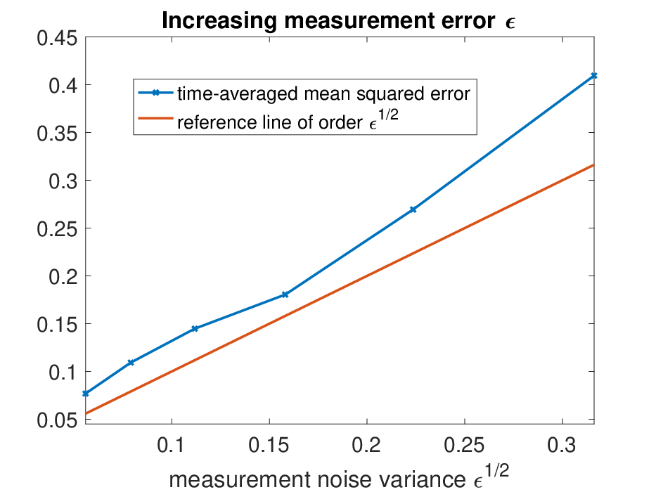
In order to emulate a continuous setting the steps size is chosen to be d​t=10−7dt=10^{-7} and the number of steps 10710^{7}. The dimension of the state space is set to be Nx=40N_{x}=40, which is a standard choice of the Lorenz 96 model. The l-EnKBF is implemented with M=10M=10 ensemble members. The results are displayed in the left panel of Figure 1. Note that the MSE is normalised with respect to the dimension, i.e., is divided by NxN_{x}. The test run confirms that the numerical growth rate with respect to an increasing ϵ\epsilon is in line with theoretical order of the expected error derived in claim OPEN1)1) of Theorem 3.4.

Refer to caption
Refer to caption

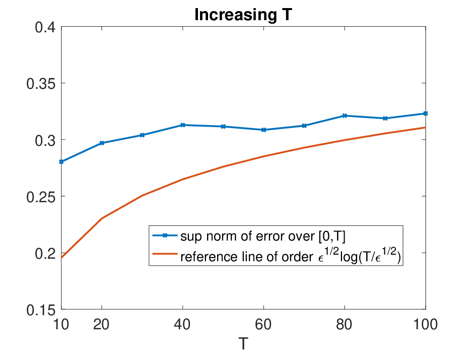
Figure 1: Time-averaged MSE as a function of the measurement error variance ϵ\epsilon is displayed in the left panel. The right panel displays the estimated supt∈[0,T]et\sup_{t\in[0,T]}e_{t} for varying TT.

4.2 High dimensional testcase

In the second test scheme, the robustness with respect to state space dimension is investigated. In particular we consider the case where the number of ensemble members MM is comparatively small and kept fixed for increasing dimensions. Thus the imbalance between ensemble size and dimension of the state space grows with increasing NxN_{x}. More precisely we run the filter for Nx∈{40,240,440,640,840,1040}N_{x}\in\{40,240,440,640,840,1040\} with M=10M=10 and ϵ=0.003125\epsilon=0.003125. The resulting time-averaged MSE after 10610^{6} steps with step size d​t=10−7dt=10^{-7} are displayed in the left panel of Figure 2. As state in claim OPEN1)1) of Theorem 3.4 the error grows linearly with NxN_{x}. Further we numerically verify that the time-averaged error of the individual components, i.e.,

1T​∑t=1T[et]i2​(t)\frac{1}{T}\sum^{T}_{t=1}[e_{t}]_{i}^{2}(t) (17)

are dimension independent (see right panel of Figure 2) as stated in claim OPEN1)1) Theorem 3.6. Note that we fixed the considered component of the state vector to be i=11i=11 while other index choice produces largely the same results.

Refer to caption
Refer to caption

Figure 2: Time-averaged MSE as a function of the state dimension NxN_{x} is displayed in the left panel whereas the time-averaged MSE for one fixed component for increasing NxN_{x} is shown in the right panel.

4.3 Uniform error for bounded time interval

In the final test scheme, we consider a setting with a growing number of steps 10610^{6} to 10710^{7} for a fixed step size d​t=10−5dt=10^{-5} resulting in filter runs for different time values T∈{10,…,100}T\in\{10,\dots,100\}. Note that the step size is set to be slightly larger than in the previous examples so that the range of considered TT values is more interesting. Further the measurement error variance is set to ϵ=0.01\epsilon=0.01 and the dimension of the state space is Nx=40N_{x}=40. We simulate the filtering process 3030 times and record the filter error ej​(t),j=1,…,30,e^{j}(t),j=1,\ldots,30, for each simulation. We plot the averaged path-wise l2l_{2}-square error up to TT, which is

130​∑j=130maxt∈[0,T]⁡‖ej​(t)‖2\frac{1}{30}\sum^{30}_{j=1}\max_{t\in[0,T]}||e^{j}(t)||^{2}

in the right panel of Figure 1. The dominating part22 2 For the considered NxN_{x}, ϵ\epsilon and TT, the other dominating component C​ϵ​NxC\sqrt{\epsilon}N_{x} is not large but can of course become significant for Nx>>0N_{x}>>0. C​ϵ​log⁡(C​T/ϵ)C\sqrt{\epsilon}\log(CT/\sqrt{\epsilon}) of the theoretical order of claim OPEN3)3) of Theorem 3.4 is plotted as a reference slope.

Note that the numerically obtain error is in line with the theoretical order and thus is verifying the logarithmic dependence of the uniform bound on time TT.

5 Conclusion

In this paper, the earlier derived stability and accuracy results for the EnKBF are extended for systems with Nx>>MN_{x}>>M via localization. Further the upper bound for the covariance is independent of the number of ensemble members MM and the derived path-wise bounds have a better scaling with respect to the time T. Moreover it is shown that the accuracy in the individual components is independent of the state dimension NxN_{x} and a Laplace type condition is obtained. Natural extensions include partially observed processes and misspecified drift functions f⁡(xt,λ)f(x_{t},\lambda) with unknown parameter λ\lambda. Moreover the presented ideas can be used for the analysis of properties of Multilevel Ensemble Kalman Filters [10, 11] or of consistent filters, such as the Ensemble Transform Particle Filter [26] or the Feedback Particle Filter [32], for finite number of ensemble members.

Acknowledgement

The research of J.d.W is funded by Deutsche Forschungsgemeinschaft (DFG) - SFB1294/1 - 318763901 Project (A02) “Long-time stability and accuracy of ensemble transform filter algorithms”. JdW was also supported by ERC Advanced Grant ÒACRCCÓ (grant 339390) and by the Simons CRM Scholar-in-Residence Program. The research of X.T.T is funded by Singapore MOE AcRF Tier 1 funding, grant number R-146-000-292-114. Further the authors would like to thank the anonymous referees for their constructive criticism.

Appendix A Proof for filter wellposedness and stability

A.1 Matrix norms and Riccati equation

To start, we have several norm inequalities which are utilized in this paper.

Lemma A.1

For any N×NN\times N matrix AA, the following holds

‖A‖max≤‖A‖,\displaystyle\|A\|_{\max}\leq\|A\|, (18)
‖A‖≤‖A‖1​‖AT‖1.\displaystyle\|A\|\leq\sqrt{\|A\|_{1}\|A^{T}\|_{1}}. (19)

Inequality (18) follows via

‖A‖max=maxi,j⁡|[A]i,j|=maxi,j⁡|[et]iT​A​ej|≤‖A‖,\|A\|_{\max}=\max_{i,j}|[A]_{i,j}|=\max_{i,j}|[e_{t}]_{i}^{T}Ae_{j}|\leq\|A\|,

where [et]i[e_{t}]_{i} and eje_{j} are the ii-th and jj-th standard Euclidean basis vector. Inequality (19) follows from [24] Lemma B.2.

Lemma A.2

Let PP, QQ and ϕ\phi be positive, symmetric and semidefinite Nx×NxN_{x}\times N_{x} matrices and [ϕ]i,i=1[\phi]_{i,i}=1 for all ii. Then

  1. 1)

    For all ii, [(P∘ϕ)​Q]i,i=[P⁡(Q∘ϕ)]i,i[(P\circ\phi)Q]_{i,i}=[P(Q\circ\phi)]_{i,i}.

  2. 2)

    If P⪯QP\preceq Q, then P∘ϕ⪯Q∘ϕP\circ\phi\preceq Q\circ\phi.

  3. 3)

    ‖P∘ϕ‖max=‖P‖max=maxi⁡{[P]i,i}\|P\circ\phi\|_{\max}=\|P\|_{\max}=\max_{i}\{[P]_{i,i}\}

  4. 4)

    ‖P∘ϕ‖≤‖P∘ϕ‖1≤Cϕ​‖P‖max\|P\circ\phi\|\leq\|P\circ\phi\|_{1}\leq C_{\phi}\|P\|_{\max}, where Cϕ=max⁡∑ji⁡|ϕi,j|C_{\phi}=\max_{i}\sum_{j}|\phi_{i,j}|.

Just note that

[(P∘ϕ)​Q]i,i=∑kPi,k​ϕi,k​Qk,i=∑kPi,k​ϕk,i​Qk,i=[P⁡(Q∘ϕ)]i,i.[(P\circ\phi)Q]_{i,i}=\sum_{k}P_{i,k}\phi_{i,k}Q_{k,i}=\sum_{k}P_{i,k}\phi_{k,i}Q_{k,i}=[P(Q\circ\phi)]_{i,i}.

Due to the linearity of the Schur product, it suffices to show that 0⪯P∘ϕ0\preceq P\circ\phi. This is known as the Schur product theorem, which can be verified using the following identity, which holds for all NxN_{x}-dimensional vectors uu, with DuD_{u} being the diagonal matrix where its diagonal entries are the same as uu:

uT​(P∘ϕ)​u=tr​(P​Du​ϕ​Du)=tr​(P12​Du​ϕ12​ϕ12​Du​P12)≥0.u^{T}(P\circ\phi)u=\text{tr}(PD_{u}\phi D_{u})=\text{tr}(P^{\frac{1}{2}}D_{u}\phi^{\frac{1}{2}}\phi^{\frac{1}{2}}D_{u}P^{\frac{1}{2}})\geq 0.

Since PP is a positive semidefinite matrix for each ii and jj, it follows that

⟨[et]i−ej,P⁡([et]i−ej)⟩=⟨[et]i,P​[et]i⟩−2​⟨[et]i,P​ej⟩+⟨ej,P​ej⟩≥0,\langle[e_{t}]_{i}-e_{j},P([e_{t}]_{i}-e_{j})\rangle=\langle[e_{t}]_{i},P[e_{t}]_{i}\rangle-2\langle[e_{t}]_{i},Pe_{j}\rangle+\langle e_{j},Pe_{j}\rangle\geq 0,

where [et]i[e_{t}]_{i} and eje_{j} are the ii and jj-th standard Euclidean basis vector. This implies

2​⟨[et]i,P​ej⟩≤⟨[et]i,P​[et]i⟩+⟨ej,P​ej⟩≤2​maxk​[P]k,k.2\langle[e_{t}]_{i},Pe_{j}\rangle\leq\langle[e_{t}]_{i},P[e_{t}]_{i}\rangle+\langle e_{j},Pe_{j}\rangle\leq 2\max_{k}[P]_{k,k}.

In other words in a positive semidefinite matrix the maximal values are reached on the diagonal. Note that the Schur product P∘ϕP\circ\phi is a positive semidefinite as well, so it’s maximal matrix entries are also assumed on the diagonal. Since ϕ\phi is set to [ϕ]i,i=1[\phi]_{i,i}=1 for all ii the Schur product does not alter the diagonal entries of PP thus ‖P∘ϕ‖max=‖P‖max\|P\circ\phi\|_{\max}=\|P\|_{\max}.

Recall that inequality (19)(\ref{eq:2normlestuff}) implies ‖A‖≤‖A‖1\|A\|\leq\|A\|_{1} for any symmetric matrix A which yields the first half of claim 4), since P∘ϕP\circ\phi is symmetric. The other half can be obtained by

‖P∘ϕ‖≤‖P∘ϕ‖1=maxi⁡|∑jϕi,j​Pi,j|≤max⁡∑ji⁡|ϕi,j|​‖P‖max=Cϕ​‖P‖max.\|P\circ\phi\|\leq\|P\circ\phi\|_{1}=\max_{i}\left|\sum_{j}\phi_{i,j}P_{i,j}\right|\leq\max_{i}\sum_{j}|\phi_{i,j}|\|P\|_{\max}=C_{\phi}\|P\|_{\max}.

In this paper, we often concern Riccati type of stochastic equation. In particular, we are often interested in finding bounds for the maximum entry of the solution. To do so, we employ a comparison principle, which generates bounds by comparing with another ODE. In particular, we have the following lemma.

Lemma A.3

Suppose Xt=[x1​(t),…,xn​(t)]X_{t}=[x_{1}(t),\ldots,x_{n}(t)] jointly follows an ODE, dd​t​Xt=F⁡(Xt)\frac{d}{dt}X_{t}=F(X_{t}). Let mt=max1≤i≤n′⁡{xi​(t)}m_{t}=\max_{1\leq i\leq n^{\prime}}\{x_{i}(t)\}, where n′n^{\prime} can be smaller than nn. Let iti_{t} be the smallest index ii such that xi​(t)=mtx_{i}(t)=m_{t}. Suppose there is a continuous function g⁡(x,t)g(x,t) such that for any t≥0t\geq 0,

dd​t​xit​(t)≤g⁡(xit​(t),t).\frac{d}{dt}x_{i_{t}}(t)\leq g(x_{i_{t}}(t),t).

Suppose yty_{t} satisfies dd​t​yt=g⁡(yt,t)+δ0\frac{d}{dt}y_{t}=g(y_{t},t)+\delta_{0} for a fixed δ0>0\delta_{0}>0 and y0>m0y_{0}>m_{0}, then the following hold

  1. 1)

    For all t>0t>0, yt>mty_{t}>m_{t}.

  2. 2)

    Suppose g⁡(x,t)=g⁡(x)=−cϵ​x2+b​x+a−δ0g(x,t)=g(x)=-\frac{c}{\epsilon}x^{2}+bx+a-\delta_{0}, where a,b,ca,b,c are constants. Let

    Δϵ:=2​b2​ϵ24​c2+a​ϵc=Θ⁡(ϵ).\Delta_{\epsilon}:=2\sqrt{\frac{b^{2}\epsilon^{2}}{4c^{2}}+\frac{a\epsilon}{c}}=\Theta(\sqrt{\epsilon}).

    If y0>0y_{0}>0, then yt≤max⁡{Δϵ,y0}y_{t}\leq\max\{\Delta_{\epsilon},y_{0}\} for all t>0t>0. Moreover, when t>t∗=c​ϵΔϵ=Θ⁡(ϵ)t>t_{*}=\frac{c\epsilon}{\Delta_{\epsilon}}=\Theta(\sqrt{\epsilon}), yt≤Δϵy_{t}\leq\Delta_{\epsilon}.

  3. 3)

    Suppose ztz_{t} is a process such that 0<zt<D0<z_{t}<D for all t>0t>0, and zt≤Δϵz_{t}\leq\Delta_{\epsilon} for t>t∗t>t_{*}, where Δϵ,t∗\Delta_{\epsilon},t_{*} are positive quantities of order Θ⁡(ϵ)\Theta(\sqrt{\epsilon}). Suppose g⁡(x,t)=α​−x​zt−βϵ​x​zt−γ−δ0g(x,t)=\alpha\sqrt{-xz_{t}}-\frac{\beta}{\epsilon}xz_{t}-\gamma-\delta_{0}, where α,β,γ\alpha,\beta,\gamma are all positive constants. Then if y0<0y_{0}<0,

    yt≤−min⁡{|y0|,γ2α2​D,γ​ϵ2​β​D},∀t>0.y_{t}\leq-\min\left\{|y_{0}|,\frac{\gamma^{2}}{\alpha^{2}D},\frac{\gamma\epsilon}{2\beta D}\right\},\quad\forall t>0.

    Moreover |yt|>cϵ|y_{t}|>c_{\epsilon} for all t>t∗+3​cϵγ=Θ⁡(ϵ)t>t_{*}+\frac{3c_{\epsilon}}{\gamma}=\Theta(\sqrt{\epsilon}), where

    cϵ:=min⁡{γ29​α2​Δϵ,γ​ϵ3​β​Δϵ}=Θ⁡(ϵ).c_{\epsilon}:=\min\left\{\frac{\gamma^{2}}{9\alpha^{2}\Delta_{\epsilon}},\frac{\gamma\epsilon}{3\beta\Delta_{\epsilon}}\right\}=\Theta(\sqrt{\epsilon}).

Let t1=inf{t>0,yt≤mt}t_{1}=\inf\{t>0,y_{t}\leq m_{t}\}. By continuity of mtm_{t} and yty_{t}, t1>0t_{1}>0. Suppose t1t_{1} is finite, then yt1=mt1y_{t_{1}}=m_{t_{1}}. Therefore

dd​t​xit1​(t1)≤g⁡(xit1​(t),t1)=g⁡(yt1,t1)=dd​t​y​(t1)−δ0.\frac{d}{dt}x_{i_{t_{1}}}(t_{1})\leq g(x_{i_{t_{1}}}(t),t_{1})=g(y_{t_{1}},t_{1})=\frac{d}{dt}y(t_{1})-\delta_{0}.

This indicate for sufficiently small δ>0\delta>0,

xit1​(t1−δ)>xit1​(t1)−δ​g​(xit1​(t),t1)−12​δ​δ0>y⁡(t1)−δ​g​(y⁡(t1),t1)+12​δ​δ0>y⁡(t1−δ).x_{i_{t_{1}}}(t_{1}-\delta)>x_{i_{t_{1}}}(t_{1})-\delta g(x_{i_{t_{1}}}(t),t_{1})-\frac{1}{2}\delta\delta_{0}>y(t_{1})-\delta g(y(t_{1}),t_{1})+\frac{1}{2}\delta\delta_{0}>y(t_{1}-\delta).

This contradicts with the definition of t1t_{1}. Therefore t1=∞t_{1}=\infty.

First we denote the root of g⁡(x,t)+δ0=0g(x,t)+\delta_{0}=0 as

y±=−b​ϵ2​c±b2​ϵ24​c2+a​ϵc.y_{\pm}=-\frac{b\epsilon}{2c}\pm\sqrt{\frac{b^{2}\epsilon^{2}}{4c^{2}}+\frac{a\epsilon}{c}}.

It is easy to check that y+>0>y−y_{+}>0>y_{-}, while Δϵ=y+−y−\Delta_{\epsilon}=y_{+}-y_{-}. Note that g⁡(x)+δ0≤0g(x)+\delta_{0}\leq 0 when yt≥Δϵ≥y+y_{t}\geq\Delta_{\epsilon}\geq y_{+}. So yty_{t} is decreasing when yty_{t} is above Δϵ\Delta_{\epsilon}.

Next note that yty_{t} is the solution of a Riccati differential equation. The solution to the Riccati ODE is given by has the explicit formulation

yt−y−yt−y+=exp⁡(cϵ​t​(y+−y−))​(y0−y−y0−y+)\frac{y_{t}-y_{-}}{y_{t}-y_{+}}=\exp\left(\frac{c}{\epsilon}t(y_{+}-y_{-})\right)\left(\frac{y_{0}-y_{-}}{y_{0}-y_{+}}\right) (20)

If y0<y+y_{0}<y_{+}, it is easy to check that (20) always take negative value, meaning yt<y+<y+−y−=Δϵy_{t}<y_{+}<y_{+}-y_{-}=\Delta_{\epsilon} for all t>0t>0. When y0>y+y_{0}>y_{+} and t>t∗t>t_{*}, from (20) leads to

yt−y−yt−y+≥exp⁡(cϵ​t​(y+−y−))≥2,\frac{y_{t}-y_{-}}{y_{t}-y_{+}}\geq\exp\left(\frac{c}{\epsilon}t(y_{+}-y_{-})\right)\geq 2,

so yt≤y+−y−=2​b2​ϵ24​c2+a​ϵc=Θ⁡(ϵ)y_{t}\leq y_{+}-y_{-}=2\sqrt{\frac{b^{2}\epsilon^{2}}{4c^{2}}+\frac{a\epsilon}{c}}=\Theta(\sqrt{\epsilon}).

Note that g⁡(x,t)+δ0<0g(x,t)+\delta_{0}<0 when |x|<min⁡{γ2α2​D,γ​ϵ2​β​D}|x|<\min\left\{\frac{\gamma^{2}}{\alpha^{2}D},\frac{\gamma\epsilon}{2\beta D}\right\}, so yty_{t} will be decreasing if it is above −min⁡{γ2α2​D,γ​ϵ2​β​D}-\min\left\{\frac{\gamma^{2}}{\alpha^{2}D},\frac{\gamma\epsilon}{2\beta D}\right\}. This leads to the first part of the claim.

Next note that when 0≥x≥−cϵ0\geq x\geq-c_{\epsilon} and t>t∗t>t_{*}, g⁡(x,t)≤−γ3g(x,t)\leq-\frac{\gamma}{3}. So yty_{t} will be decreasing with rate at least γ3\frac{\gamma}{3} when 0≥yt≥−cϵ0\geq y_{t}\geq-c_{\epsilon} and t>t∗t>t_{*}, this leads to our claim.

A.2 Upper bounds for sample covariance

Recall that PtP_{t} is positive semidefinite, therefore by Lemma A.2

‖Pt‖max=max⁡{[Pt]i,i,i=1,…,Nx},\|P_{t}\|_{\max}=\max\{[P_{t}]_{i,i},i=1,\ldots,N_{x}\},

where the components of PtP_{t} follows an ODE (13). Therefore, in order to apply Lemma A.3 Claim 1), it suffices to investigate the ODE deriving the component with the maximal value. Suppose at time tt, [Pt]k,k=‖Pt‖max[P_{t}]_{k,k}=\|P_{t}\|_{\max} for certain kk. Considering the time evolution of [PtL]k,k[P^{L}_{t}]_{k,k} given by (13), it is given by

dd​t​[Pt]k,k=[Ft+FtT]k,k+[Pt†​Pt+Pt​Pt†]k,k−12​ϵ​[PtL​Ω​Pt+Pt​Ω​PtL]k,k.\frac{d}{dt}[P_{t}]_{k,k}=[F_{t}+F_{t}^{T}]_{k,k}+[P_{t}^{\dagger}P_{t}+P_{t}P_{t}^{\dagger}]_{k,k}-\frac{1}{2\epsilon}[P^{L}_{t}\Omega P_{t}+P_{t}\Omega P^{L}_{t}]_{k,k}. (21)

First note that [Ft]k,k=1M−1​∑i(xki−x¯k)​(fk​(Xti)−f¯k)[F_{t}]_{k,k}=\frac{1}{M-1}\sum_{i}(x^{i}_{k}-\overline{x}_{k})(f_{k}(X^{i}_{t})-\overline{f}_{k}), where by Assumption 2.1 we have

|fk​(Xi)−f¯k|≤1M​∑j=1M|fk​(Xti)−fk​(Xtj)|≤1M​∑j=1M∑l=1Nxℱ𝐝⁡(k,l)​|xli−xlj|.|f_{k}(X^{i})-\overline{f}_{k}|\leq\frac{1}{M}\sum_{j=1}^{M}|f_{k}(X^{i}_{t})-f_{k}(X^{j}_{t})|\leq\frac{1}{M}\sum_{j=1}^{M}\sum_{l=1}^{N_{x}}\mathcal{F}_{\mathbf{d}(k,l)}|x^{i}_{l}-x^{j}_{l}|.

This leads to

[Ft]k,k\displaystyle[F_{t}]_{k,k} ≤1M−1∑i=1M|xki−x¯k∥fk(Xti)−f¯k|\displaystyle\leq\frac{1}{M-1}\sum_{i=1}^{M}|x^{i}_{k}-\overline{x}_{k}\|f_{k}(X_{t}^{i})-\overline{f}_{k}|
≤1(M−1)​M​∑i,j,l,mℱ𝐝⁡(k,l)​|xki−xkm|​|xli−xlj|\displaystyle\leq\frac{1}{(M-1)M}\sum_{i,j,l,m}\mathcal{F}_{\mathbf{d}(k,l)}|x^{i}_{k}-x^{m}_{k}||x^{i}_{l}-x^{j}_{l}|
≤∑l=1Nxℱ𝐝⁡(k,l)​∑i,m|xki−xkm|2M⁡(M−1)​∑i,j|xli−xlj|2M⁡(M−1)\displaystyle\leq\sum_{l=1}^{N_{x}}\mathcal{F}_{\mathbf{d}(k,l)}\sqrt{\frac{\sum_{i,m}|x^{i}_{k}-x^{m}_{k}|^{2}}{M(M-1)}}\sqrt{\frac{\sum_{i,j}|x^{i}_{l}-x^{j}_{l}|^{2}}{M(M-1)}}
≤∑l=1Nxℱ𝐝⁡(k,l)​[Pt]k,k≤Cf​[Pt]k,k.\displaystyle\leq\sum_{l=1}^{N_{x}}\mathcal{F}_{\mathbf{d}(k,l)}[P_{t}]_{k,k}\leq C_{f}[P_{t}]_{k,k}. (22)

Also, note that [Pt†​Pt]k,k=[Pt†]k,k​[Pt]k,k=1[P_{t}^{\dagger}P_{t}]_{k,k}=[P_{t}^{\dagger}]_{k,k}[P_{t}]_{k,k}=1 due to Defintion 2.2, so

[Pt†​Pt]k,k=1.[P_{t}^{\dagger}P_{t}]_{k,k}=1. (23)

Lastly, we have

[PtL​Ω​Pt]k,k=∑i=1Nx[PtL]k,i​Ωi,i​[Pt]i,k=∑i=1Nx[Pt]k,i2​ϕi,k​Ωi,i≥Ωk,k​[Pt]k,k2≥ωmin​[Pt]k,k2.[P_{t}^{L}\Omega P_{t}]_{k,k}=\sum_{i=1}^{N_{x}}[P_{t}^{L}]_{k,i}\Omega_{i,i}[P_{t}]_{i,k}=\sum_{i=1}^{N_{x}}[P_{t}]^{2}_{k,i}\phi_{i,k}\Omega_{i,i}\geq\Omega_{k,k}[P_{t}]^{2}_{k,k}\geq\omega_{\min}[P_{t}]^{2}_{k,k}. (24)

Insert (22),(23) and (24) to (21), we find

dd​t​[Pt]k,k≤2​Cf​[Pt]k,k+2−ωminϵ​[Pt]k,k2.\frac{d}{dt}[P_{t}]_{k,k}\leq 2C_{f}[P_{t}]_{k,k}+2-\frac{\omega_{\min}}{\epsilon}[P_{t}]_{k,k}^{2}.

Therefore Lemma A.3 claim 1) applies with

g⁡(x,t)=2​Cf​x+2−ωminϵ​x2.g(x,t)=2C_{f}x+2-\frac{\omega_{\min}}{\epsilon}x^{2}.

Let δ0=1\delta_{0}=1, Lemma A.3 claim 2) yields the result of this lemma.

A.3 Lower bounds for sample covariance

The proof is similar to the one of Lemma 3.1, but we need to change sign, because

−‖Pt‖min=max⁡{−[Pt]i,i,i=1,…,Nx}.-\|P_{t}\|_{\min}=\max\{-[P_{t}]_{i,i},i=1,\ldots,N_{x}\}.

By Lemma A.3 claim 1), we assume at time tt, ‖Pt‖min=[Pt]k,k\|P_{t}\|_{\min}=[P_{t}]_{k,k} and investigate the ODE that −[Pt]k,k-[P_{t}]_{k,k} follows. It is given by the inverse of (21). Following same procedures prior to (22), we have

[Ft]k,k≥−∑l=1Nxℱ𝐝⁡(k,l)∑i,m|xki−xkm|2M⁡(M−1)∑i,j|xli−xlj|2M⁡(M−1)≥−Cf[Pt]k,k​‖Pt‖max[F_{t}]_{k,k}\geq-\sum_{l=1}^{N_{x}}\mathcal{F}_{\mathbf{d}(k,l)}\sqrt{\frac{\sum_{i,m}|x^{i}_{k}-x^{m}_{k}|^{2}}{M(M-1)}}\sqrt{\frac{\sum_{i,j}|x^{i}_{l}-x^{j}_{l}|^{2}}{M(M-1)}}\geq-C_{f}\sqrt{[P_{t}]_{k,k}\|P_{t}\|_{\max}} (25)

(23) remains the same. Finally recall that in (24), we have

[PtL​Ω​Pt]k,k=∑i=1Nx[Pt]k,i2​ϕi,k​Ωi,i≤∑i=1Nxωmax​ϕi,k​[Pt]k,k​‖Pt‖max≤ωmax​Cϕ​[Pt]k,k​‖Pt‖max.[P_{t}^{L}\Omega P_{t}]_{k,k}=\sum_{i=1}^{N_{x}}[P_{t}]^{2}_{k,i}\phi_{i,k}\Omega_{i,i}\leq\sum_{i=1}^{N_{x}}\omega_{\max}\phi_{i,k}[P_{t}]_{k,k}\|P_{t}\|_{\max}\leq\omega_{\max}C_{\phi}[P_{t}]_{k,k}\|P_{t}\|_{\max}. (26)

Insert (25), (23), and (26) into (21), we find

−dd​t​[Pt]k,k≤2​Cf​−(−[Pt]k,k)​‖Pt‖max+ωmaxϵ​Cϕ​‖Pt‖max​[Pt]k,k−2.-\frac{d}{dt}[P_{t}]_{k,k}\leq 2C_{f}\sqrt{-(-[P_{t}]_{k,k})\|P_{t}\|_{\max}}+\frac{\omega_{\max}}{\epsilon}C_{\phi}\|P_{t}\|_{\max}[P_{t}]_{k,k}-2.

So we can apply Lemma A.3 claim 3) with δ0=1\delta_{0}=1 and

g⁡(x,t)=2​Cf​−x​‖Pt‖max+ωmaxϵ​Cϕ​x​[Pt]k,k−2.g(x,t)=2C_{f}\sqrt{-x\|P_{t}\|_{\max}}+\frac{\omega_{\max}}{\epsilon}C_{\phi}x[P_{t}]_{k,k}-2.

This gives us the claimed result.

Appendix B Proof for filter error analysis in l2l_{2} norm

B.1 Evolution of component-wise error

Before we prove the statements of Theorem 3.4 we consider the following auxiliary lemma which will be used several times throughout the remainder of the paper.

Lemma B.1

Let [et]j[e_{t}]_{j} be the jj-th component of the filter error ete_{t}. Then the following holds

d​[et]j2≤\displaystyle d[e_{t}]^{2}_{j}\leq (−αt​[et]j2−2​ϵ−1​∑i=1j[Pt∘ϕ~]j,i​[et]i​[et]j+∑i≠jℱ𝐝⁡(i,j)​|[et]i|2+βt)​d​t+d​[ℳt]j.\displaystyle\Big(-\alpha_{t}[e_{t}]_{j}^{2}-2\epsilon^{-1}\sum_{i=1}^{j}[P_{t}\circ\tilde{\phi}]_{j,i}[e_{t}]_{i}[e_{t}]_{j}+\sum_{i\neq j}\mathcal{F}_{\mathbf{d}(i,j)}|[e_{t}]_{i}|^{2}+\beta_{t}\Big)dt+d[\mathcal{M}_{t}]_{j}. (27)

In (27), ℳt\mathcal{M}_{t} is a NxN_{x} dimensional martingale with components being

d[ℳt]j=22[et]jdWj−2ϵ−1/2[et]j[PtLΩ1/2dB]j.d[\mathcal{M}_{t}]_{j}=2\sqrt{2}[e_{t}]_{j}dW_{j}-2\epsilon^{-1/2}[e_{t}]_{j}[P^{L}_{t}\Omega^{1/2}dB]_{j}.

In (27), αt\alpha_{t} and βt\beta_{t} are two real valued processes given by

αt\displaystyle\alpha_{t} :=2​ϵ−1​ρ​‖Pt‖min−Cf−1,\displaystyle:=2\epsilon^{-1}\rho\|P_{t}\|_{\min}-C_{f}-1,
βt\displaystyle\beta_{t} :=Cf2​‖Pt‖max+2+ϵ−1​Cϕ2​ωmax​‖Pt‖max2.\displaystyle:=C^{2}_{f}\|P_{t}\|_{\max}+2+\epsilon^{-1}C_{\phi}^{2}\omega_{\max}\|P_{t}\|^{2}_{\max}.

By Lemmas 3.1 and 3.2, the following holds for all t≥0t\geq 0

αt≥α∗=−Cf−1,\alpha_{t}\geq\alpha^{*}=-C_{f}-1,
βt≤β∗:=Cf2​max​{‖P0‖max,λmax}+2+ϵ−1​Cϕ2​ωmax​max​{‖P0‖max2,λmax2}=Θ⁡(ϵ−1).\beta_{t}\leq\beta^{*}:=C^{2}_{f}\max\{\|P_{0}\|_{\max},\lambda_{\max}\}+2+\epsilon^{-1}C_{\phi}^{2}\omega_{\max}\max\{\|P_{0}\|^{2}_{\max},\lambda^{2}_{\max}\}=\Theta(\epsilon^{-1}).

When t≥t∗t\geq t_{*}, these bounds can be further improved to

αt≥α∗\displaystyle\alpha_{t}\geq\alpha_{*} :=2​ϵ−1​ρ​λmin−Cf−1=𝒪⁡(ϵ−12),\displaystyle:=2\epsilon^{-1}\rho\lambda_{\min}-C_{f}-1=\mathcal{O}(\epsilon^{-\frac{1}{2}}),
βt≤β∗\displaystyle\beta_{t}\leq\beta_{*} :=Cf2​λmax+2+ϵ−1​Cϕ2​ωmax​λmax2=Θ⁡(1).\displaystyle:=C^{2}_{f}\lambda_{\max}+2+\epsilon^{-1}C_{\phi}^{2}\omega_{\max}\lambda^{2}_{\max}=\Theta(1).

Recall the evolution of XtX_{t} and X¯t\overline{X}_{t} are given by d​Xt=f⁡(Xt)​d​t+2​d​WtdX_{t}=f(X_{t})dt+\sqrt{2}dW_{t} and

dX¯t=f¯tdt−ϵ−1PtLΩ(X¯tdt−dYt)=f¯tdt−ϵ−1PtLΩ(X¯tdt−Xtdt−ϵΩ−1/2dBt).d\overline{X}_{t}=\overline{f}_{t}dt-\epsilon^{-1}P^{L}_{t}\Omega(\overline{X}_{t}dt-dY_{t})=\overline{f}_{t}dt-\epsilon^{-1}P^{L}_{t}\Omega(\overline{X}_{t}dt-X_{t}dt-\sqrt{\epsilon}\Omega^{-1/2}dB_{t}).

The evolution of the error et=Xt−X¯te_{t}=X_{t}-\overline{X}_{t} is given by the difference between the two, namely

det=(f(Xt)−f¯t−ϵ−1PtLΩet)dt+2dWt−ϵ−1/2PtLΩ1/2dBt.de_{t}=(f(X_{t})-\overline{f}_{t}-\epsilon^{-1}P^{L}_{t}\Omega e_{t})dt+\sqrt{2}dW_{t}-\epsilon^{-1/2}P_{t}^{L}\Omega^{1/2}dB_{t}.

The jj-th component of this differential equation is given by

d[et]j=(fj(Xt)−f¯j−ϵ−1[PtLΩet]j)dt+2dWj−ϵ−1/2[PtLΩ1/2dB]j,d[e_{t}]_{j}=(f_{j}(X_{t})-\overline{f}_{j}-\epsilon^{-1}[P_{t}^{L}\Omega e_{t}]_{j})dt+\sqrt{2}dW_{j}-\epsilon^{-1/2}[P^{L}_{t}\Omega^{1/2}dB]_{j},

where f¯j\overline{f}_{j} denotes the j-th component of f¯t\overline{f}_{t}. Ito’s formula implies that

d​[et]j2=\displaystyle d[e_{t}]^{2}_{j}= (2​(fj​(Xt)−f¯j−ϵ−1​[PtL​Ω​et]j)​[et]j+2+ϵ−1​[PtL​Ω​PtL]j​j)​d​t\displaystyle\left(2(f_{j}(X_{t})-\overline{f}_{j}-\epsilon^{-1}[P_{t}^{L}\Omega e_{t}]_{j})[e_{t}]_{j}+2+\epsilon^{-1}[P^{L}_{t}\Omega P^{L}_{t}]_{jj}\right)dt
+22[et]jdWj−ϵ−1/22[et]j[PtLΩ1/2dB]j.\displaystyle+2\sqrt{2}[e_{t}]_{j}dW_{j}-\epsilon^{-1/2}2[e_{t}]_{j}[P^{L}_{t}\Omega^{1/2}dB]_{j}. (28)

To continue, note that

|fj​(Xt)−f¯j|​|[et]j|\displaystyle|f_{j}(X_{t})-\overline{f}_{j}||[e_{t}]_{j}| =|fj​(Xt)−1M​∑i=1Mfj​(Xti)|​|[et]j|\displaystyle=\left|f_{j}(X_{t})-\frac{1}{M}\sum_{i=1}^{M}f_{j}(X^{i}_{t})\right|\,|[e_{t}]_{j}|
≤1M∑i=1M|fj(Xt)−fj(Xti)∥[et]j|\displaystyle\leq\frac{1}{M}\sum_{i=1}^{M}|f_{j}(X_{t})-f_{j}(X^{i}_{t})\|[e_{t}]_{j}|
≤1M∑i=1M|fj(X¯t)−fj(Xti)∥[et]j|+|fj(Xt)−fj(X¯t)∥[et]j|.\displaystyle\leq\frac{1}{M}\sum_{i=1}^{M}|f_{j}(\overline{X}_{t})-f_{j}(X^{i}_{t})\|[e_{t}]_{j}|+|f_{j}(X_{t})-f_{j}(\overline{X}_{t})\|[e_{t}]_{j}|. (29)

By Assumption 2.1, the second part of (29) can be bounded easily by

|fj(Xt)−fj(X¯t)∥[et]j|≤∑i=1Nxℱ𝐝⁡(i,j)|[Xt−X¯t]i∥[et]j|=∑i=1Nxℱ𝐝⁡(i,j)|[et]i||[et]j|≤12Cf|[et]j|2+12∑i≠jℱ𝐝⁡(i,j)|[et]i|2.|f_{j}(X_{t})-f_{j}(\overline{X}_{t})\|[e_{t}]_{j}|\leq\sum_{i=1}^{N_{x}}\mathcal{F}_{\mathbf{d}(i,j)}|[X_{t}-\overline{X}_{t}]_{i}\|[e_{t}]_{j}|=\sum_{i=1}^{N_{x}}\mathcal{F}_{\mathbf{d}(i,j)}|[e_{t}]_{i}||[e_{t}]_{j}|\leq\frac{1}{2}C_{f}|[e_{t}]_{j}|^{2}+\frac{1}{2}\sum_{i\neq j}\mathcal{F}_{\mathbf{d}(i,j)}|[e_{t}]_{i}|^{2}. (30)

To bound the first part of (29), we note by Assumption 2.1 and Cauchy Schwarz,

1M​∑i=1M|fj​(X¯t)−fj​(Xti)|\displaystyle\frac{1}{M}\sum_{i=1}^{M}|f_{j}(\overline{X}_{t})-f_{j}(X^{i}_{t})| ≤∑i,k=1M,Nxℱ𝐝⁡(k,j)M​|[Xti−X¯t]k|\displaystyle\leq\sum_{i,k=1}^{M,N_{x}}\frac{\mathcal{F}_{\mathbf{d}(k,j)}}{M}|[X^{i}_{t}-\overline{X}_{t}]_{k}|
≤∑k=1Nxℱ𝐝⁡(k,j)M2​∑i=1M|[Xti−X¯t]k|2\displaystyle\leq\sqrt{\sum_{k=1}^{N_{x}}\frac{\mathcal{F}_{\mathbf{d}(k,j)}}{M^{2}}\sum_{i=1}^{M}|[X^{i}_{t}-\overline{X}_{t}]_{k}|^{2}}
≤1M​Cf2​(M−1)​[Pt]k,k≤Cf​‖Pt‖max12.\displaystyle\leq\sqrt{\frac{1}{M}C_{f}^{2}(M-1)[P_{t}]_{k,k}}\leq C_{f}\|P_{t}\|^{\frac{1}{2}}_{\max}. (31)

Then multiplication with |[et]j||[e_{t}]_{j}| with (31) yields

1M∑i=1M|fj(X¯t)−fj(Xti)∥[et]j|\displaystyle\frac{1}{M}\sum_{i=1}^{M}|f_{j}(\overline{X}_{t})-f_{j}(X^{i}_{t})\|[e_{t}]_{j}| ≤12​(1M​∑i=1M|fj​(X¯t)−fj​(Xti)|)2+12​|[et]j|2\displaystyle\leq\frac{1}{2}(\frac{1}{M}\sum_{i=1}^{M}|f_{j}(\overline{X}_{t})-f_{j}(X^{i}_{t})|)^{2}+\frac{1}{2}|[e_{t}]_{j}|^{2}
≤12​Cf2​‖Pt‖max+12​|[et]j|2.\displaystyle\leq\frac{1}{2}C^{2}_{f}\|P_{t}\|_{\max}+\frac{1}{2}|[e_{t}]_{j}|^{2}.

Plug these into (29), we find

|fj​(Xt)−f¯j|​|[et]j|≤12​Cf2​‖Pt‖max+12​|[et]j|2+12​Cf​|[et]j|2+12​∑i≠jℱ𝐝⁡(i,j)​|[et]i|2.|f_{j}(X_{t})-\overline{f}_{j}||[e_{t}]_{j}|\leq\frac{1}{2}C^{2}_{f}\|P_{t}\|_{\max}+\frac{1}{2}|[e_{t}]_{j}|^{2}+\frac{1}{2}C_{f}|[e_{t}]_{j}|^{2}+\frac{1}{2}\sum_{i\neq j}\mathcal{F}_{\mathbf{d}(i,j)}|[e_{t}]_{i}|^{2}. (32)

Next, we deal with [PtL​Ω​et]j[P_{t}^{L}\Omega e_{t}]_{j} in (28). Define ϕ~:=ϕ−ρ​I\tilde{\phi}:=\phi-\rho I and obtain the following equality

[PtL​Ω​et]j=∑i=1Nx[Pt∘ϕ]j,i​Ωi,i​[et]i=ρ​[Pt]j,j​Ωj,j​[et]j+∑i=1Nx[Pt∘ϕ~]j,i​Ωi,i​[et]i.[P_{t}^{L}\Omega e_{t}]_{j}=\sum_{i=1}^{N_{x}}[P_{t}\circ\phi]_{j,i}\Omega_{i,i}[e_{t}]_{i}=\rho[P_{t}]_{j,j}\Omega_{j,j}[e_{t}]_{j}+\sum_{i=1}^{N_{x}}[P_{t}\circ\tilde{\phi}]_{j,i}\Omega_{i,i}[e_{t}]_{i}. (33)

Also note that

[PtL​Ω​PtL]j,j=∑iΩi,i​ϕi,j2​[Pt]i,j2≤‖Pt‖max2​ωmax​∑iϕi,j2≤Cϕ2​ωmax​‖Pt‖max2.[P^{L}_{t}\Omega P^{L}_{t}]_{j,j}=\sum_{i}\Omega_{i,i}\phi^{2}_{i,j}[P_{t}]^{2}_{i,j}\leq\|P_{t}\|_{\max}^{2}\omega_{\max}\sum_{i}\phi^{2}_{i,j}\leq C_{\phi}^{2}\omega_{\max}\|P_{t}\|_{\max}^{2}. (34)

Plug (34), (33), and (32) into (28), we obtain

d​[et]j2≤((1+CLOSECLOSE\displaystyle d[e_{t}]^{2}_{j}\leq\Big((1+ OPENCf−2​ϵ−1​ρ​‖Pt‖min)​[et]j2−2​ϵ−1​∑i=1Nx[Pt∘ϕ~]j,i​[et]i​[et]j\displaystyle C_{f}-2\epsilon^{-1}\rho\|P_{t}\|_{\min})[e_{t}]_{j}^{2}-2\epsilon^{-1}\sum_{i=1}^{N_{x}}[P_{t}\circ\tilde{\phi}]_{j,i}[e_{t}]_{i}[e_{t}]_{j} (35)
+∑i≠jℱ𝐝⁡(i,j)|[et]i|2+Cf2∥Pt∥max+2+ϵ−1Cϕ2ωmax∥Pt∥max2)dt\displaystyle+\sum_{i\neq j}\mathcal{F}_{\mathbf{d}(i,j)}|[e_{t}]_{i}|^{2}+C_{f}^{2}\|P_{t}\|_{\max}+2+\epsilon^{-1}C_{\phi}^{2}\omega_{\max}\|P_{t}\|_{\max}^{2}\Big)dt
+22[et]jdWj−2ϵ−1/2[et]j[PtLΩ1/2dB]j.\displaystyle\quad+2\sqrt{2}[e_{t}]_{j}dW_{j}-2\epsilon^{-1/2}[e_{t}]_{j}[P^{L}_{t}\Omega^{1/2}dB]_{j}.

B.2 Two technical lemmas

Lemma B.2 (Grönwall’s inequality)

Suppose a real value process utu_{t} satisfies the following for t≥t0t\geq t_{0} and constants α\alpha and β\beta:

d​ut≤(−α​ut+β)​d​t+d​Mtdu_{t}\leq(-\alpha u_{t}+\beta)dt+dM_{t}

for some martingale MtM_{t}. It follows that for any t≥t0t\geq t_{0}

𝔼t0​ut≤ut0​exp⁡(−α⁡(t−t0))+βα​(1−exp⁡(−α⁡(t−t0))).\mathbb{E}_{t_{0}}u_{t}\leq u_{t_{0}}\exp(-\alpha(t-t_{0}))+\frac{\beta}{\alpha}(1-\exp(-\alpha(t-t_{0}))).

When α\alpha and β\beta are both positive, we have further that

𝔼t0​ut≤ut0​exp⁡(−α⁡(t−t0))+βα.\mathbb{E}_{t_{0}}u_{t}\leq u_{t_{0}}\exp(-\alpha(t-t_{0}))+\frac{\beta}{\alpha}.

Consider ut′=exp⁡(α⁡(t−t0))​utu^{\prime}_{t}=\exp(\alpha(t-t_{0}))u_{t}. Then its evolution follows

d​ut′=α​ut​d​t+exp⁡(α⁡(t−t0))​d​ut≤exp⁡(α⁡(t−t0))​β+exp⁡(α⁡(t−t0))​d​Mt.du^{\prime}_{t}=\alpha u_{t}dt+\exp(\alpha(t-t_{0}))du_{t}\leq\exp(\alpha(t-t_{0}))\beta+\exp(\alpha(t-t_{0}))dM_{t}.

Integrating both hands from t0t_{0} to tt, then take conditional expectation we have

𝔼t0​ut′=ut0′+βα​(exp⁡(α⁡(t−t0))−1).\mathbb{E}_{t_{0}}u^{\prime}_{t}=u^{\prime}_{t_{0}}+\frac{\beta}{\alpha}(\exp(\alpha(t-t_{0}))-1).

This leads to our claim.

Lemma B.3

For a positive random variable XX, if there are constants A≥2,B≥0A\geq 2,B\geq 0 such that ℙ⁡(X>M)≤A​exp⁡(−λ​M)+exp⁡(λ​B−λ​M)\mathbb{P}(X>M)\leq A\exp(-\lambda M)+\exp(\lambda B-\lambda M) holds for all M>0M>0, then

𝔼⁡[X]≤1+log⁡2​Aλ+B.\mathbb{E}[X]\leq\frac{1+\log 2A}{\lambda}+B.

Note that if we let C=1λ​log⁡A+BC=\frac{1}{\lambda}\log A+B, which is the point the quantile upper bound takes value 11,

𝔼⁡[X]=∫0∞ℙ⁡(X>x)​𝑑x\displaystyle\mathbb{E}[X]=\int^{\infty}_{0}\mathbb{P}(X>x)dx =∫C∞ℙ⁡(X>x)​𝑑x+∫0Cℙ⁡(X>x)​𝑑x\displaystyle=\int^{\infty}_{C}\mathbb{P}(X>x)dx+\int^{C}_{0}\mathbb{P}(X>x)dx
≤∫C∞(A+exp⁡(λ​B))​exp⁡(−λ​x)​𝑑x+∫0C1​𝑑x\displaystyle\leq\int^{\infty}_{C}(A+\exp(\lambda B))\exp(-\lambda x)dx+\int^{C}_{0}1dx
=A+exp⁡(λ​B)λ​exp⁡(−λ​C)+C=1+log⁡(A+exp⁡(λ​B))λ.\displaystyle=\frac{A+\exp(\lambda B)}{\lambda}\exp(-\lambda C)+C=\frac{1+\log(A+\exp(\lambda B))}{\lambda}.

Finally, since A≤A​exp⁡(λ​B),exp⁡(λ​B)≤A​exp⁡(λ​B)A\leq A\exp(\lambda B),\exp(\lambda B)\leq A\exp(\lambda B), so log⁡(A+exp⁡(λ​B)≤λ​B+log⁡2​ACLOSE\log(A+\exp(\lambda B)\leq\lambda B+\log 2A.

B.3 Proof of Theorem 3.4

Note that ϕ~⪰0\tilde{\phi}\succeq 0 and thus ∑i,j[Pt∘ϕ~]j,i​[et]i​[et]j≥0\sum_{i,j}[P_{t}\circ\tilde{\phi}]_{j,i}[e_{t}]_{i}[e_{t}]_{j}\geq 0, and ∑iℱ𝐝⁡(i,j)≤Cf\sum_{i}\mathcal{F}_{\mathbf{d}(i,j)}\leq C_{f}. So utilizing Lemma B.1 and summing over all jj on both sides of (27) yields

d​‖et‖2≤(Cf−αt)​‖et‖2​d​t+Nx​βt​d​t+d​ℳt′,d\|e_{t}\|^{2}\leq\left(C_{f}-\alpha_{t}\right)\|e_{t}\|^{2}dt+N_{x}\beta_{t}dt+d\mathcal{M}_{t}^{\prime}, (36)

where the martingale is given by

dℳt′=∑j=1Nx22[et]jdWj−2r−1/2[et]j[PsLΩ1/2dB]j=22etTdWt−2r−1/2etTPtLΩ1/2dBt.\displaystyle d\mathcal{M}^{\prime}_{t}=\sum_{j=1}^{N_{x}}2\sqrt{2}[e_{t}]_{j}dW_{j}-2r^{-1/2}[e_{t}]_{j}[P^{L}_{s}\Omega^{1/2}dB]_{j}=2\sqrt{2}e_{t}^{T}dW_{t}-2r^{-1/2}e_{t}^{T}P^{L}_{t}\Omega^{1/2}dB_{t}.

For t∈[0,t∗]t\in[0,t_{*}], (36) can be further upper-bounded by

d​‖et‖2≤(Cf−α∗)​‖et‖2​d​t+Nx​β∗​d​t+d​ℳt′.d\|e_{t}\|^{2}\leq\left(C_{f}-\alpha^{*}\right)\|e_{t}\|^{2}dt+N_{x}\beta^{*}dt+d\mathcal{M}_{t}^{\prime}.

Employing Gronwall’s inequality, there is a constant DD such that

𝔼​‖et∗‖2≤exp⁡((2​Cf+1)​t∗)​𝔼​‖e0‖2+Nx​β∗​exp⁡((2​Cf+1)​t∗)−12​Cf+1=Θ⁡(ϵ−1).\mathbb{E}\|e_{t_{*}}\|^{2}\leq\exp((2C_{f}+1)t_{*})\mathbb{E}\|e_{0}\|^{2}+N_{x}\beta^{*}\frac{\exp((2C_{f}+1)t_{*})-1}{2C_{f}+1}=\Theta(\epsilon^{-1}).

For t≥t∗t\geq t_{*}, (36) can be further upper-bounded by

d​‖et‖2≤−α∗′​‖et‖2​d​t+Nx​β∗​d​t+d​ℳt′.d\|e_{t}\|^{2}\leq-\alpha^{\prime}_{*}\|e_{t}\|^{2}dt+N_{x}\beta_{*}dt+d\mathcal{M}_{t}^{\prime}.

Employing Gronwall’s inequality, we find that with α∗′=α∗−Cf\alpha_{*}^{\prime}=\alpha_{*}-C_{f},

𝔼​‖et‖2≤𝔼​‖et∗‖2​exp⁡(−α∗′​(t−t∗))+Nx​β∗α∗′​(1−exp⁡(−α∗′​(t−t∗))).\mathbb{E}\|e_{t}\|^{2}\leq\mathbb{E}\|e_{t_{*}}\|^{2}\exp(-\alpha_{*}^{\prime}(t-t_{*}))+\frac{N_{x}\beta_{*}}{\alpha_{*}^{\prime}}(1-\exp(-\alpha_{*}^{\prime}(t-t_{*}))). (37)

Since α∗′=α∗−Cf=Θ(ϵ−1/2)\alpha_{*}^{\prime}=\alpha_{*}-C_{f}=\Theta(\epsilon^{-1/2}), β∗=𝒪⁡(1)\beta_{*}=\mathcal{O}(1), and ϵ−1exp(−λϵ−1/2)=o(1)\epsilon^{-1}\exp(-\lambda\epsilon^{-1/2})=o(1) for any λ>0\lambda>0, so we have proved for claim 1).

First we note the quadratic variation of the martingale term ℳt′\mathcal{M}_{t}^{\prime} is given by

dd​t​⟨ℳ′⟩t=8​‖et‖2+4​ϵ−1​‖Ω1/2​PtL​et‖2≤(8+4​ϵ−1​ωmax​‖PtL‖2)​‖et‖2.\frac{d}{dt}\langle\mathcal{M}^{\prime}\rangle_{t}=8\|e_{t}\|^{2}+4\epsilon^{-1}\|\Omega^{1/2}P^{L}_{t}e_{t}\|^{2}\leq(8+4\epsilon^{-1}\omega_{\max}\|P^{L}_{t}\|^{2})\|e_{t}\|^{2}.

So by Ito’s formula on exp⁡(λ​‖et‖2)\exp(\lambda\|e_{t}\|^{2}), the following holds with αt′=αt−Cf\alpha_{t}^{\prime}=\alpha_{t}-C_{f},

d​exp⁡(CLOSE\displaystyle d\exp( OPENλ​‖et‖2)≤((−λ​αt′​‖et‖2+λ​βt​Nx)​d​t+λ​d​ℳt′)​exp⁡(λ​‖et‖2)+12​λ2​exp⁡(λ​‖et‖2)​d​⟨ℳ⟩t​d​t\displaystyle\lambda\|e_{t}\|^{2})\leq((-\lambda\alpha^{\prime}_{t}\|e_{t}\|^{2}+\lambda\beta_{t}N_{x})dt+\lambda d\mathcal{M}_{t}^{\prime})\exp(\lambda\|e_{t}\|^{2})+\frac{1}{2}\lambda^{2}\exp(\lambda\|e_{t}\|^{2})d\langle\mathcal{M}\rangle_{t}dt
≤(−γt​‖et‖2+λ​βt​Nx)​exp⁡(λ​‖et‖2)​d​t+λ​exp⁡(λ​‖et‖2)​d​ℳt′.\displaystyle\leq(-\gamma_{t}\|e_{t}\|^{2}+\lambda\beta_{t}N_{x})\exp(\lambda\|e_{t}\|^{2})dt+\lambda\exp(\lambda\|e_{t}\|^{2})d\mathcal{M}_{t}^{\prime}.

where

γt=λ​αt′−4​λ2−2​λ2​ωmax​ϵ−1​‖PtL‖2.\gamma_{t}=\lambda\alpha^{\prime}_{t}-4\lambda^{2}-2\lambda^{2}\omega_{\max}\epsilon^{-1}\|P^{L}_{t}\|^{2}.

By Lemma 3.1 and 3.2, we have for all t>0t>0

−γt≤γ∗=λ⁡(2​Cf+1)+4​λ2+2​λ2​ωmax​Cϕ2​max⁡{‖P0‖max2,λmax2},-\gamma_{t}\leq\gamma^{*}=\lambda(2C_{f}+1)+4\lambda^{2}+2\lambda^{2}\omega_{\max}C_{\phi}^{2}\max\{\|P_{0}\|^{2}_{\max},\lambda_{\max}^{2}\},

and for t≥t∗t\geq t_{*}

λ≤λ∗=α∗′8+4​ωmax​Cϕ2​λmax2=Θ(ϵ−1/2).\lambda\leq\lambda_{*}=\frac{\alpha^{\prime}_{*}}{8+4\omega_{\max}C_{\phi}^{2}\lambda_{\max}^{2}}=\Theta(\epsilon^{-1/2}).
γt≥λ​α∗′−4​λ2−2​λ2​ωmax​Cϕ2​λmax2≥12​λ​α∗′.\gamma_{t}\geq\lambda\alpha^{\prime}_{*}-4\lambda^{2}-2\lambda^{2}\omega_{\max}C_{\phi}^{2}\lambda_{\max}^{2}\geq\frac{1}{2}\lambda\alpha^{\prime}_{*}.

For t≤t∗t\leq t_{*}, by Gronwall’s inequality we have

𝔼​exp⁡(λ​‖et∗‖2)≤exp⁡((γ∗+λ​β∗​Nx)​t∗)​exp⁡(λ​‖e0‖2).\mathbb{E}\exp(\lambda\|e_{t_{*}}\|^{2})\leq\exp((\gamma^{*}+\lambda\beta^{*}N_{x})t_{*})\exp(\lambda\|e_{0}\|^{2}). (38)

And when t≥t∗t\geq t_{*},

d​exp⁡(λ​‖et‖2)≤(λ​β∗​Nx−12​λ​α∗′​‖et‖2)​exp⁡(λ​‖et‖2)​d​t+λ​exp⁡(λ​‖et‖2)​d​ℳt′.d\exp(\lambda\|e_{t}\|^{2})\leq(\lambda\beta_{*}N_{x}-\frac{1}{2}\lambda\alpha^{\prime}_{*}\|e_{t}\|^{2})\exp(\lambda\|e_{t}\|^{2})dt+\lambda\exp(\lambda\|e_{t}\|^{2})d\mathcal{M}_{t}^{\prime}. (39)

Note that when 14​λ​α∗′​‖et‖2≤λ​β∗​Nx\frac{1}{4}\lambda\alpha^{\prime}_{*}\|e_{t}\|^{2}\leq\lambda\beta_{*}N_{x},

exp⁡(λ​‖et‖2)≤exp⁡(4​λ​Nx​β∗α∗′),\exp(\lambda\|e_{t}\|^{2})\leq\exp\left(\frac{4\lambda N_{x}\beta_{*}}{\alpha^{\prime}_{*}}\right),

we obtain

(λ​β∗​Nx−12​λ​α∗′​‖et‖2)​exp⁡(λ​‖et‖2)≤−λ​β∗​Nx​exp⁡(λ​‖et‖2)+2​λ​β∗​Nx​exp⁡(4​λ​Nx​β∗α∗′).(\lambda\beta_{*}N_{x}-\tfrac{1}{2}\lambda\alpha^{\prime}_{*}\|e_{t}\|^{2})\exp(\lambda\|e_{t}\|^{2})\leq-\lambda\beta_{*}N_{x}\exp(\lambda\|e_{t}\|^{2})+2\lambda\beta_{*}N_{x}\exp\left(\frac{4\lambda N_{x}\beta_{*}}{\alpha^{\prime}_{*}}\right).

Otherwise, when 14​λ​α∗′​‖et‖2≥λ​β∗​Nx\frac{1}{4}\lambda\alpha^{\prime}_{*}\|e_{t}\|^{2}\geq\lambda\beta_{*}N_{x}, we have

(λ​β∗​Nx−12​λ​α∗′​‖et‖2)​exp⁡(λ​‖et‖2)≤−14​λ​α∗′​‖et‖2​exp⁡(λ​‖et‖2)≤−λ​β∗​Nx​exp⁡(λ​‖et‖2).(\lambda\beta_{*}N_{x}-\tfrac{1}{2}\lambda\alpha^{\prime}_{*}\|e_{t}\|^{2})\exp(\lambda\|e_{t}\|^{2})\leq-\frac{1}{4}\lambda\alpha^{\prime}_{*}\|e_{t}\|^{2}\exp(\lambda\|e_{t}\|^{2})\leq-\lambda\beta_{*}N_{x}\exp(\lambda\|e_{t}\|^{2}).

In summary, we always have

(λ​β∗​Nx−12​λ​α∗′​‖et‖2)​exp⁡(λ​‖et‖2)≤−λ​β∗​Nx​exp⁡(λ​‖et‖2)+2​λ​β∗​Nx​exp⁡(4​λ​Nx​β∗α∗′).(\lambda\beta_{*}N_{x}-\tfrac{1}{2}\lambda\alpha^{\prime}_{*}\|e_{t}\|^{2})\exp(\lambda\|e_{t}\|^{2})\leq-\lambda\beta_{*}N_{x}\exp(\lambda\|e_{t}\|^{2})+2\lambda\beta_{*}N_{x}\exp\left(\frac{4\lambda N_{x}\beta_{*}}{\alpha^{\prime}_{*}}\right). (40)

Inserting (40) in (39) yields

d​exp⁡(λ​‖et‖2)≤[−λ​β∗​Nx​exp⁡(λ​‖et‖2)+2​λ​β∗​Nx​exp⁡(4​λ​Nx​β∗α∗′)]​d​t+λ​exp⁡(λ​‖et‖2)​d​ℳt′.d\exp(\lambda\|e_{t}\|^{2})\leq\Big[-\lambda\beta_{*}N_{x}\exp(\lambda\|e_{t}\|^{2})+2\lambda\beta_{*}N_{x}\exp\left(\frac{4\lambda N_{x}\beta_{*}}{\alpha^{\prime}_{*}}\right)\Big]dt+\lambda\exp(\lambda\|e_{t}\|^{2})d\mathcal{M}_{t}^{\prime}.

After applying Grönwall’s inequality and (38) we obtain the following

𝔼⁡[exp⁡(λ​‖et‖2)]\displaystyle\mathbb{E}[\exp(\lambda\|e_{t}\|^{2})] ≤exp⁡(−λ​β∗​Nx​(t−t∗))​𝔼​[exp⁡(λ​‖et∗‖2)]+2​exp⁡(4​λ​Nx​β∗α∗)\displaystyle\leq\exp{(-\lambda\beta_{*}N_{x}(t-t_{*}))}\mathbb{E}[\exp(\lambda\|e_{t_{*}}\|^{2})]+2\exp\left(\frac{4\lambda N_{x}\beta_{*}}{\alpha_{*}}\right)
≤exp⁡(−(γ∗+λ​β∗​Nx)​t∗−λ​β∗​Nx​(t−t∗))​𝔼​[exp⁡(λ​‖e0‖2)]+2​exp⁡(4​λ​Nx​β∗α∗′).\displaystyle\leq\exp(-(\gamma^{*}+\lambda\beta^{*}N_{x})t_{*}-\lambda\beta_{*}N_{x}(t-t_{*}))\mathbb{E}[\exp(\lambda\|e_{0}\|^{2})]+2\exp\left(\frac{4\lambda N_{x}\beta_{*}}{\alpha^{\prime}_{*}}\right).

When t→∞t\to\infty, this leads to claim 2):

lim supt→∞𝔼​exp⁡(λ​‖et‖2)≤2​exp⁡(4​λ​Nx​β∗α∗′).\limsup_{t\to\infty}\mathbb{E}\exp(\lambda\|e_{t}\|^{2})\leq 2\exp\left(\frac{4\lambda N_{x}\beta_{*}}{\alpha_{*}^{\prime}}\right).

We consider function

g⁡(x)=(λ​β∗​Nx−12​λ​α∗′​x)​exp⁡(λ​x)g(x)=(\lambda\beta_{*}N_{x}-\frac{1}{2}\lambda\alpha^{\prime}_{*}x)\exp(\lambda x)

By finding the critical point, it is easy to see

g(x)≤g(2​β∗​Nxα∗′−1λ)=α∗′2​𝕖exp(2​λ∗​β​Nxα∗′)=:G∗=Θ(ϵ−1/2)g(x)\leq g\Big(\frac{2\beta_{*}N_{x}}{\alpha^{\prime}_{*}}-\frac{1}{\lambda}\Big)=\frac{\alpha^{\prime}_{*}}{2\mathbb{e}}\exp\Big(\frac{2\lambda_{*}\beta N_{x}}{\alpha^{\prime}_{*}}\Big)=:G_{*}=\Theta(\epsilon^{-1/2})

Combine this with (39), we find

d​exp⁡(λ​‖et‖2)≤G∗​d​t+λ​exp⁡(λ​‖et‖2)​d​ℳt′,∀t≥t∗.d\exp(\lambda\|e_{t}\|^{2})\leq G_{*}dt+\lambda\exp(\lambda\|e_{t}\|^{2})d\mathcal{M}_{t}^{\prime},\quad\forall t\geq t_{*}.

So by Dynkin’s formula, if we let τ=min{t:t≥t0,∥et∥2≥M}\tau=\min\{t:t\geq t_{0},\|e_{t}\|^{2}\geq M\}, then

𝔼t0​exp⁡(λ​‖eT∧τ‖2)≤exp⁡(λ​‖et0‖2)+𝔼​∫t0T∧τG∗​𝑑t≤exp⁡(λ​‖et0‖2)+G∗​T.\mathbb{E}_{t_{0}}\exp(\lambda\|e_{T\wedge\tau}\|^{2})\leq\exp(\lambda\|e_{t_{0}}\|^{2})+\mathbb{E}\int^{T\wedge\tau}_{t_{0}}G_{*}dt\leq\exp(\lambda\|e_{t_{0}}\|^{2})+G_{*}T.

By Markov inequality we have

ℙ⁡(maxt0≤t≤T⁡‖et‖2≥M)=ℙt0\displaystyle\mathbb{P}(\max_{t_{0}\leq t\leq T}\|e_{t}\|^{2}\geq M)=\mathbb{P}_{t_{0}} (‖eT∧τ‖2≥M)≤𝔼t0​exp⁡(λ​‖eT∧τ‖2)exp⁡(λ​M)\displaystyle(\|e_{T\wedge\tau}\|^{2}\geq M)\leq\frac{\mathbb{E}_{t_{0}}\exp(\lambda\|e_{T\wedge\tau}\|^{2})}{\exp(\lambda M)}
≤α∗′​T2​𝕖​exp⁡(2​λ​β∗​Nxα∗′−λ​M)+exp⁡(λ​‖et0‖2−λ​M).\displaystyle\leq\frac{\alpha_{*}^{\prime}T}{2\mathbb{e}}\exp\left(\frac{2\lambda\beta_{*}N_{x}}{\alpha_{*}^{\prime}}-\lambda M\right)+\exp(\lambda\|e_{t_{0}}\|^{2}-\lambda M).

Then by Lemma B.3,

𝔼t0​maxt0≤t≤T​‖eT‖2≤1λ+2​β∗​Nxα∗′+1λ​log⁡(α∗′​T𝕖)+1λ+‖et0‖.\mathbb{E}_{t_{0}}\max_{t_{0}\leq t\leq T}\|e_{T}\|^{2}\leq\frac{1}{\lambda}+\frac{2\beta_{*}N_{x}}{\alpha_{*}^{\prime}}+\frac{1}{\lambda}\log\left(\frac{\alpha^{\prime}_{*}T}{\mathbb{e}}\right)+\frac{1}{\lambda}+\|e_{t_{0}}\|.

We take λ=λ∗=Θ⁡(ϵ−12)\lambda=\lambda_{*}=\Theta(\epsilon^{-\frac{1}{2}}) to obtain our claimed result.

Appendix C Proof for component-wise filter error analysis

C.1 Component-wise Lyapunov weights

In order to bound [et]i2[e_{t}]^{2}_{i} in long time, it is necessary to build a Lyapunov function for it. The main challenge here is that dynamics of [et]i2[e_{t}]^{2}_{i} is coupled with the error of other components. The idea is here to find a weight vector viv^{i} so that Eti=∑jvji​[et]j2E^{i}_{t}=\sum_{j}v^{i}_{j}[e_{t}]^{2}_{j} is a Lyapunov function. The design of viv^{i} happens to relate to the structure of ϕ\phi, and can be expressed as the Green function of a Markov chain.

Lemma C.1

Under Assumption 3.5. Let TT be a random variable of geometric-qq distribution, that is

ℙ(T=n)=(1−q)qn−1,n=1,2,….\mathbb{P}(T=n)=(1-q)q^{n-1},\quad n=1,2,\ldots.

Consider a Markov chain XtX_{t} on the points {1,…,Nx}\{1,\ldots,N_{x}\}. Its transition probability is given by

ℙ⁡(Xt+1=j|Xt=i)={1q​ϕi,jj≠i1−1q​∑j≠iϕi,jj=i.\mathbb{P}(X_{t+1}=j|X_{t}=i)=\begin{cases}\frac{1}{q}\phi_{i,j}\quad&j\neq i\\ 1-\frac{1}{q}\sum_{j\neq i}\phi_{i,j}\quad&j=i.\end{cases}

Fix an index i∈{1,…,Nx}i\in\{1,\ldots,N_{x}\}. Define vector viv^{i}, where its components are given by

vji=𝔼⁡(∑k=1T𝟏Xk=i|X1=j).v^{i}_{j}=\mathbb{E}\left(\sum^{T}_{k=1}\mathbf{1}_{X_{k}=i}\bigg|X_{1}=j\right).

Then viv^{i} satisfies the following properties

  1. 1)

    vji≥0,∀jv^{i}_{j}\geq 0,\forall j and in specific vii≥1−qv^{i}_{i}\geq 1-q.

  2. 2)

    For all index jj, ∑l≠jϕj,l​vli≤vji\sum_{l\neq j}\phi_{j,l}v^{i}_{l}\leq v^{i}_{j}.

  3. 3)

    ∑j=1Nxvji≤1\sum_{j=1}^{N_{x}}v^{i}_{j}\leq 1.

Since ∑k=1T𝟏Xk=i≥0\sum^{T}_{k=1}\mathbf{1}_{X_{k}=i}\geq 0 a.s., so vji≥0v^{i}_{j}\geq 0. Moreover,

vii=𝔼⁡(∑k=1T𝟏Xk=i|X1=i)≥𝔼⁡(𝟏T=1,X1=i|X1=i)=1−q.v^{i}_{i}=\mathbb{E}\left(\sum^{T}_{k=1}\mathbf{1}_{X_{k}=i}\bigg|X_{1}=i\right)\geq\mathbb{E}\left(\mathbf{1}_{T=1,X_{1}=i}\bigg|X_{1}=i\right)=1-q.

Next, by doing a first step analysis of Markov chain, we find that

vji=(1−q)⋅𝟏j=i+q(1−1q∑l≠jϕj,l)vji+q⋅1q∑l≠jϕj,lvli.v^{i}_{j}=(1-q)\cdot\mathbf{1}_{j=i}+q\left(1-\frac{1}{q}\sum_{l\neq j}\phi_{j,l}\right)v^{i}_{j}+q\cdot\frac{1}{q}\sum_{l\neq j}\phi_{j,l}v^{i}_{l}. (41)

Since ∑l≠jϕj,l≤q<1\sum_{l\neq j}\phi_{j,l}\leq q<1, we have

vji≥∑l≠jϕl,j​vli.v^{i}_{j}\geq\sum_{l\neq j}\phi_{l,j}v^{i}_{l}.

We sum (41) over all jj and obtain

∑j=1Nxvji\displaystyle\sum_{j=1}^{N_{x}}v^{i}_{j} =(1−q)+q​∑j=1Nx(1−1q​∑l≠jϕj,l)​vji+∑j=1Nx∑l≠jϕj,l​vli\displaystyle=(1-q)+q\sum_{j=1}^{N_{x}}\left(1-\frac{1}{q}\sum_{l\neq j}\phi_{j,l}\right)v^{i}_{j}+\sum_{j=1}^{N_{x}}\sum_{l\neq j}\phi_{j,l}v^{i}_{l}
≤1−q+∑j=1Nx∑l≠jϕj,l​vli=1−q+∑l=1Nxvli​(∑j≠lϕj,l).\displaystyle\leq 1-q+\sum_{j=1}^{N_{x}}\sum_{l\neq j}\phi_{j,l}v^{i}_{l}=1-q+\sum_{l=1}^{N_{x}}v_{l}^{i}\left(\sum_{j\neq l}\phi_{j,l}\right).

Therefore we have

(1−q)​∑j=1Nxvji≤∑j=1Nx(1−∑j≠lϕj,l)​vji≤1−q,(1-q)\sum_{j=1}^{N_{x}}v^{i}_{j}\leq\sum_{j=1}^{N_{x}}(1-\sum_{j\neq l}\phi_{j,l})v^{i}_{j}\leq 1-q,

which leads to our claim.

C.2 Proof of Theorem 3.6

Recall that Lemma B.1 has shown that

d​[et]i2≤\displaystyle d[e_{t}]^{2}_{i}\leq (−αt​[et]i2−2​ϵ−1​∑j=1[Pt∘ϕ~]i,j​[et]i​[et]j+∑j≠iℱ𝐝⁡(i,j)​|[et]j|2+βt)​d​t+d​[ℳt]i.\displaystyle\Big(-\alpha_{t}[e_{t}]_{i}^{2}-2\epsilon^{-1}\sum_{j=1}[P_{t}\circ\tilde{\phi}]_{i,j}[e_{t}]_{i}[e_{t}]_{j}+\sum_{j\neq i}\mathcal{F}_{\mathbf{d}(i,j)}|[e_{t}]_{j}|^{2}+\beta_{t}\Big)dt+d[\mathcal{M}_{t}]_{i}. (42)

Recall that ϕ~=ϕ−ρ​I\tilde{\phi}=\phi-\rho I. In the following, we use Pj,iP_{j,i} to denote the (j,i)(j,i)-th component of PtP_{t}. Then by Cauchy Schwartz and Young’s inequality

−2​[Pt∘ϕ~]i,j​[et]i​[et]j=−2​ϕj,i​Pj,i​[et]i​[et]j\displaystyle-2[P_{t}\circ\tilde{\phi}]_{i,j}[e_{t}]_{i}[e_{t}]_{j}=-2\phi_{j,i}P_{j,i}[e_{t}]_{i}[e_{t}]_{j} ≤−2​ϕj,i​Pj,j​[et]j​Pi,i​[et]i\displaystyle\leq-2\phi_{j,i}\sqrt{P_{j,j}}[e_{t}]_{j}\sqrt{P_{i,i}}[e_{t}]_{i}
≤ϕi,j​(Pj,j​[et]j2+Pi,i​[et]i2), for ​j≠i.\displaystyle\leq\phi_{i,j}(P_{j,j}[e_{t}]_{j}^{2}+P_{i,i}[e_{t}]_{i}^{2}),\quad\text{ for }j\neq i.

Then note that

−2​Pi,i​ϕi,i​[et]i2+∑i≠jϕi,j​Pi,i​[et]i2≤(q−2)​Pi,i​[et]i2<−Pi,i​[et]i2,-2P_{i,i}\phi_{i,i}[e_{t}]_{i}^{2}+\sum_{i\neq j}\phi_{i,j}P_{i,i}[e_{t}]_{i}^{2}\leq(q-2)P_{i,i}[e_{t}]_{i}^{2}<-P_{i,i}[e_{t}]_{i}^{2},

so (42) leads to

d​[et]i2≤(∑j≠i(ℱ𝐝⁡(i,j)+ϵ−1​ϕi,j​Pj,j)​[et]j2−αt​[et]i2−ϵ−1​Pi,i​[et]i2+βt)​d​t+d​[ℳt]i.d[e_{t}]^{2}_{i}\leq\left(\sum_{j\neq i}(\mathcal{F}_{\mathbf{d}(i,j)}+\epsilon^{-1}\phi_{i,j}P_{j,j})[e_{t}]^{2}_{j}-\alpha_{t}[e_{t}]_{i}^{2}-\epsilon^{-1}P_{i,i}[e_{t}]_{i}^{2}+\beta_{t}\right)dt+d[\mathcal{M}_{t}]_{i}.\\ (43)

We denote the vector Et=[e12,e22,⋯eN2]TE_{t}=[e_{1}^{2},e_{2}^{2},\cdots e_{N}^{2}]^{T}. Further we define vector viv^{i}, of which the component is given by Lemma C.1. Denote

Eti=⟨vi,Et⟩,ℳti=⟨vi,ℳt⟩.E^{i}_{t}=\langle v^{i},E_{t}\rangle,\quad\mathcal{M}^{i}_{t}=\langle v^{i},\mathcal{M}_{t}\rangle.

Then the SDE of EtiE^{i}_{t} can be bounded by a linear combination of (43), which is

d​Eti\displaystyle dE^{i}_{t} ≤∑j=1Nx(−αt​vji​[et]j2−ϵ−1​vji​(Pj,j​[et]j2−∑l≠jϕj,l​Pl,l​el2)+∑l≠jvji​ℱ𝐝⁡(j,l)​el2)+βt+d​ℳti\displaystyle\leq\sum_{j=1}^{N_{x}}\left(-\alpha_{t}v^{i}_{j}[e_{t}]_{j}^{2}-\epsilon^{-1}v^{i}_{j}(P_{j,j}[e_{t}]_{j}^{2}-\sum_{l\neq j}\phi_{j,l}P_{l,l}e^{2}_{l})+\sum_{l\neq j}v^{i}_{j}\mathcal{F}_{\mathbf{d}(j,l)}e_{l}^{2}\right)+\beta_{t}+d\mathcal{M}^{i}_{t}
=∑j=1Nx(−αt​vji​[et]j2−ϵ−1​(vji​Pj,j​[et]j2−∑l≠jvli​ϕl,j​Pj,j​[et]j2)+∑l≠jℱ𝐝⁡(j,l)​vli​[et]j2)+βt+d​ℳti\displaystyle=\sum_{j=1}^{N_{x}}\left(-\alpha_{t}v^{i}_{j}[e_{t}]_{j}^{2}-\epsilon^{-1}(v^{i}_{j}P_{j,j}[e_{t}]_{j}^{2}-\sum_{l\neq j}v^{i}_{l}\phi_{l,j}P_{j,j}[e_{t}]^{2}_{j})+\sum_{l\neq j}\mathcal{F}_{\mathbf{d}(j,l)}v^{i}_{l}[e_{t}]_{j}^{2}\right)+\beta_{t}+d\mathcal{M}^{i}_{t}
≤∑j=1Nx(−αt​vji​[et]j2​vji+Cℱ​ϕj,l​vli​[et]j2)+βt+d​ℳti.\displaystyle\leq\sum_{j=1}^{N_{x}}\left(-\alpha_{t}v^{i}_{j}[e_{t}]_{j}^{2}v^{i}_{j}+C_{\mathcal{F}}\phi_{j,l}v^{i}_{l}[e_{t}]_{j}^{2}\right)+\beta_{t}+d\mathcal{M}^{i}_{t}. (44)
≤∑j=1Nx(−αt+Cℱ)​vji​[et]j2+βt+d​ℳti=(−αt+Cℱ)​Eti+βt+d​ℳti.\displaystyle\leq\sum_{j=1}^{N_{x}}(-\alpha_{t}+C_{\mathcal{F}})v^{i}_{j}[e_{t}]_{j}^{2}+\beta_{t}+d\mathcal{M}^{i}_{t}=(-\alpha_{t}+C_{\mathcal{F}})E^{i}_{t}+\beta_{t}+d\mathcal{M}^{i}_{t}. (45)

We have used claim 3) and 2) of Lemma C.1 at (44) and (45).

Between time 00 and tϵt_{\epsilon}, recall the upper bound in Lemma B.1, apply Gronwall’s inequality

𝔼​Etϵi≤exp⁡((Cℱ−α∗)​tϵ)​(𝔼​E0i+β∗Cℱ−α∗).\mathbb{E}E^{i}_{t_{\epsilon}}\leq\exp((C_{\mathcal{F}}-\alpha^{*})t_{\epsilon})\left(\mathbb{E}E^{i}_{0}+\frac{\beta^{*}}{C_{\mathcal{F}}-\alpha^{*}}\right).

Then after tϵt_{\epsilon}, for any tt, apply Gronwall’s inequality

𝔼​Eti\displaystyle\mathbb{E}E^{i}_{t} ≤exp⁡((Cℱ−α∗)​tϵ)​𝔼​Etϵi+β∗α∗−Cℱ\displaystyle\leq\exp((C_{\mathcal{F}}-\alpha_{*})t_{\epsilon})\mathbb{E}E^{i}_{t_{\epsilon}}+\frac{\beta_{*}}{\alpha_{*}-C_{\mathcal{F}}}
≤exp⁡(Cℱ​t−α∗​tϵ−α∗​(t−tϵ))​(𝔼​E0i+β∗Cℱ−α∗)+β∗α∗−Cℱ.\displaystyle\leq\exp(C_{\mathcal{F}}t-\alpha^{*}t_{\epsilon}-\alpha_{*}(t-t_{\epsilon}))\left(\mathbb{E}E^{i}_{0}+\frac{\beta^{*}}{C_{\mathcal{F}}-\alpha^{*}}\right)+\frac{\beta_{*}}{\alpha_{*}-C_{\mathcal{F}}}.

Recall that in Lemma B.1, α∗=Θ(ϵ−1/2),β∗=Θ(ϵ−1),α∗=β∗=Θ(1)\alpha_{*}=\Theta(\epsilon^{-1/2}),\beta^{*}=\Theta(\epsilon^{-1}),\alpha^{*}=\beta_{*}=\Theta(1). So if t>t0t>t_{0}, for certain constants cc and CC

−(Cℱt−α∗tϵ−α∗(t−tϵ))≥cϵ−1/2,𝔼E0i≤maxi{|[et]i(0)|2}∑jvji≤C,-(C_{\mathcal{F}}t-\alpha^{*}t_{\epsilon}-\alpha_{*}(t-t_{\epsilon}))\geq c\epsilon^{-1/2},\quad\mathbb{E}E^{i}_{0}\leq\max_{i}\{|[e_{t}]_{i}(0)|^{2}\}\sum_{j}v^{i}_{j}\leq C,
β∗Cℱ−α∗≤C​ϵ−1,β∗α∗−Cℱ≤C​ϵ1/2.\frac{\beta^{*}}{C_{\mathcal{F}}-\alpha^{*}}\leq C\epsilon^{-1},\quad\frac{\beta_{*}}{\alpha_{*}-C_{\mathcal{F}}}\leq C\epsilon^{1/2}.

Therefore when ϵ\epsilon is small enough, 𝔼​Eti≤2​C​ϵ\mathbb{E}E^{i}_{t}\leq 2C\sqrt{\epsilon}, which is our claim 1).

First recall the individual martingale driving EtiE^{i}_{t} is given by

d​ℳti\displaystyle d\mathcal{M}^{i}_{t} =∑jvji8[et]jdWj−2vjiϵ−1/2[et]j[PtLΩ1/2dB]j.\displaystyle=\sum_{j}v^{i}_{j}\sqrt{8}[e_{t}]_{j}dW_{j}-2v^{i}_{j}\epsilon^{-1/2}[e_{t}]_{j}[P^{L}_{t}\Omega^{1/2}dB]_{j}.

The corresponding quadratic variation is bounded by

dd​t​⟨ℳi⟩t\displaystyle\frac{d}{dt}\langle\mathcal{M}^{i}\rangle_{t} =8​∑j=1Nx[et]j2​(vji)2+4​ϵ−1​∑j=1Nx(vji)2​[et]j2​∑l=1Nx[PtL]j,l2​[Ω]l,l\displaystyle=8\sum_{j=1}^{N_{x}}[e_{t}]_{j}^{2}(v^{i}_{j})^{2}+4\epsilon^{-1}\sum_{j=1}^{N_{x}}(v_{j}^{i})^{2}[e_{t}]_{j}^{2}\sum_{l=1}^{N_{x}}[P^{L}_{t}]^{2}_{j,l}[\Omega]_{l,l}
≤8​∑j=1Nx[et]j2​vji+4​ωmax​ϵ−1​‖Pt‖max2​∑j=1Nxvji​[et]j2≤4​βt​Eti.\displaystyle\leq 8\sum_{j=1}^{N_{x}}[e_{t}]_{j}^{2}v^{i}_{j}+4\omega_{\max}\epsilon^{-1}\|P_{t}\|_{\max}^{2}\sum_{j=1}^{N_{x}}v_{j}^{i}[e_{t}]_{j}^{2}\leq 4\beta_{t}E^{i}_{t}.

Denote αt′=αt−Cℱ\alpha^{\prime}_{t}=\alpha_{t}-C_{\mathcal{F}}, (which is slightly different from the one in the proof of Theorem 3.4) then recall from (45) we have

d​Eti≤−αt′​Eti​d​t+βt​d​t+d​ℳti.dE^{i}_{t}\leq-\alpha^{\prime}_{t}E^{i}_{t}dt+\beta_{t}dt+d\mathcal{M}_{t}^{i}.

By Ito’s formula on exp⁡(λ​Eti)\exp(\lambda E_{t}^{i}), we have

d​exp⁡(λ​Eti)\displaystyle d\exp(\lambda E_{t}^{i}) OPEN≤(−12​λ​αt′​Eti+4​λ​βt)​d​t+λ​d​ℳti)​exp⁡(λ​Eti)+12​λ2​exp⁡(λ​Eti)​d​⟨ℳi⟩t\displaystyle\leq(-\frac{1}{2}\lambda\alpha^{\prime}_{t}E^{i}_{t}+4\lambda\beta_{t})dt+\lambda d\mathcal{M}^{i}_{t})\exp(\lambda E^{i}_{t})+\frac{1}{2}\lambda^{2}\exp(\lambda E^{i}_{t})d\langle\mathcal{M}^{i}\rangle_{t}
≤(−12​(λ​αt′−4​λ2​βt)​Eti+λ​βt)​exp⁡(λ​Eti)​d​t+λ​exp⁡(λ​Eti)​d​ℳti.\displaystyle\leq(-\frac{1}{2}(\lambda\alpha^{\prime}_{t}-4\lambda^{2}\beta_{t})E^{i}_{t}+\lambda\beta_{t})\exp(\lambda E^{i}_{t})dt+\lambda\exp(\lambda E^{i}_{t})d\mathcal{M}^{i}_{t}. (46)

From time 00 to tϵt_{\epsilon}, by Lemma B.1,

αt′=αt−Cℱ≥α∗−Cℱ,βt≤β∗,\alpha_{t}^{\prime}=\alpha_{t}-C_{\mathcal{F}}\geq\alpha^{*}-C_{\mathcal{F}},\quad\beta_{t}\leq\beta^{*},

by Gronwall’s inequality, for all ii

𝔼​exp⁡(λ​Etϵi)≤exp⁡(tϵ​(−12​λ​(α∗−Cℱ)+2​λ2​β∗+12​λ​β∗))​exp⁡(λ​maxi​{|eti​(0)|2})<∞.\mathbb{E}\exp(\lambda E_{t_{\epsilon}}^{i})\leq\exp(t_{\epsilon}(-\tfrac{1}{2}\lambda(\alpha^{*}-C_{\mathcal{F}})+2\lambda^{2}\beta^{*}+\tfrac{1}{2}\lambda\beta^{*}))\exp(\lambda\max_{i}\{|e^{i}_{t}(0)|^{2}\})<\infty. (47)

When t>tϵt>t_{\epsilon}, Lemma B.1 further shows that

αt′=αt−Cℱ≥α∗′:=α∗−Cℱ,βt≤β∗.\alpha_{t}^{\prime}=\alpha_{t}-C_{\mathcal{F}}\geq\alpha_{*}^{\prime}:=\alpha_{*}-C_{\mathcal{F}},\quad\beta_{t}\leq\beta_{*}.

Consider λ≤λ∗=α∗′8​β∗\lambda\leq\lambda_{*}=\frac{\alpha^{\prime}_{*}}{8\beta_{*}}, then

−12​(λ​α∗−4​λ2​β∗)=−14​λ​α∗.-\frac{1}{2}(\lambda\alpha_{*}-4\lambda^{2}\beta_{*})=-\frac{1}{4}\lambda\alpha_{*}.

Then for t>tϵt>t_{\epsilon} and λ<λϵ\lambda<\lambda_{\epsilon}, we have the following upper bound from (46)

d​exp⁡(λ​Eti)≤(−14​λ​α∗′​Eti+λ​β∗)​exp⁡(λ​Eti)​d​t+λ​exp⁡(λ​Eti)​d​ℳti.d\exp(\lambda E_{t}^{i})\leq(-\frac{1}{4}\lambda\alpha^{\prime}_{*}E^{i}_{t}+\lambda\beta_{*})\exp(\lambda E^{i}_{t})dt+\lambda\exp(\lambda E^{i}_{t})d\mathcal{M}^{i}_{t}. (48)

When ϵ\epsilon is small enough, α∗′>0\alpha^{\prime}_{*}>0. Then if 18​λ​α∗′​Eti≤λ​β∗\frac{1}{8}\lambda\alpha^{\prime}_{*}E^{i}_{t}\leq\lambda\beta_{*},

(−14​λ​α∗′​Eti+λ​β∗)​exp⁡(λ​Eti)+18​λ​α∗′​exp⁡(λ​Eti)≤2​λ​β∗​exp⁡(8​λ​β∗/α∗′).(-\frac{1}{4}\lambda\alpha^{\prime}_{*}E^{i}_{t}+\lambda\beta_{*})\exp(\lambda E^{i}_{t})+\frac{1}{8}\lambda\alpha^{\prime}_{*}\exp(\lambda E^{i}_{t})\leq 2\lambda\beta_{*}\exp(8\lambda\beta_{*}/\alpha^{\prime}_{*}).

If 18​λ​α∗′​Eti≥λ​β∗\frac{1}{8}\lambda\alpha^{\prime}_{*}E^{i}_{t}\geq\lambda\beta_{*},

(−14​λ​α∗′​Eti+λ​β∗)​exp⁡(λ​Eti)≤−18​λ​α∗′​exp⁡(λ​Eti).(-\frac{1}{4}\lambda\alpha^{\prime}_{*}E^{i}_{t}+\lambda\beta_{*})\exp(\lambda E^{i}_{t})\leq-\frac{1}{8}\lambda\alpha^{\prime}_{*}\exp(\lambda E^{i}_{t}).

In summary, we always have

(−14​λ​α∗′​Eti+λ​β∗)​exp⁡(λ​Eti)≤−18​λ​α∗′​exp⁡(λ​Eti)+2​λ​β∗​exp⁡(8​λ​β∗/α∗′).(-\frac{1}{4}\lambda\alpha^{\prime}_{*}E^{i}_{t}+\lambda\beta_{*})\exp(\lambda E^{i}_{t})\leq-\frac{1}{8}\lambda\alpha^{\prime}_{*}\exp(\lambda E^{i}_{t})+2\lambda\beta_{*}\exp(8\lambda\beta_{*}/\alpha^{\prime}_{*}).

Plug this into (48), we have

d​exp⁡(λ​Eti)≤(−18​λ​α∗′​exp⁡(λ​Eti)+2​λ​β∗​exp⁡(8​λ​β∗/α∗′))​d​t+λ​exp⁡(λ​Eti)​d​ℳti.d\exp(\lambda E_{t}^{i})\leq(-\frac{1}{8}\lambda\alpha^{\prime}_{*}\exp(\lambda E^{i}_{t})+2\lambda\beta_{*}\exp(8\lambda\beta_{*}/\alpha^{\prime}_{*}))dt+\lambda\exp(\lambda E^{i}_{t})d\mathcal{M}^{i}_{t}. (49)

So Gronwall’s inequality and implies for t≥tϵt\geq t_{\epsilon}

𝔼​exp⁡(λ​Eti)≤exp⁡(−18​λ​α∗′​(t−tϵ))​𝔼​exp⁡(λ​Etϵi)+16​β∗α∗′​exp⁡(8​λ​β∗/α∗′)\displaystyle\mathbb{E}\exp(\lambda E_{t}^{i})\leq\exp(-\tfrac{1}{8}\lambda\alpha^{\prime}_{*}(t-t_{\epsilon}))\mathbb{E}\exp(\lambda E_{t_{\epsilon}}^{i})+16\frac{\beta_{*}}{\alpha^{\prime}_{*}}\exp(8\lambda\beta_{*}/\alpha^{\prime}_{*})

The first term on the right converges to zero as t→∞t\to\infty because of bound (47). We have our claim 2) because of β∗=Θ⁡(1)\beta_{*}=\Theta(1), α∗′=Θ(ϵ−1/2)\alpha^{\prime}_{*}=\Theta(\epsilon^{-1/2}), moreover Eti≥vii​[et]i2≥(1−q)​[et]i2E_{t}^{i}\geq v^{i}_{i}[e_{t}]^{2}_{i}\geq(1-q)[e_{t}]^{2}_{i} by Lemma C.1 claim 1).

We consider function

g⁡(x)=(−14​λ​α∗′​x+λ​β∗)​exp⁡(λ​x)g(x)=(-\tfrac{1}{4}\lambda\alpha^{\prime}_{*}x+\lambda\beta_{*})\exp(\lambda x)

and by finding the critical point, it is easy to see

g⁡(x)≤g⁡(4​β∗α∗′−1λ)=α∗4​𝕖​exp⁡(4​λ​β∗α∗′)=:G∗.g(x)\leq g\left(\frac{4\beta_{*}}{\alpha^{\prime}_{*}}-\frac{1}{\lambda}\right)=\frac{\alpha_{*}}{4\mathbb{e}}\exp\left(\frac{4\lambda\beta_{*}}{\alpha_{*}^{\prime}}\right)=:G_{*}.

Plug this into (48), we find for all t>t0t>t_{0},

d​exp⁡(λ​Eti)≤G∗​d​t+λ​exp⁡(λ​Eti)​d​ℳti.d\exp(\lambda E^{i}_{t})\leq G_{*}dt+\lambda\exp(\lambda E^{i}_{t})d\mathcal{M}^{i}_{t}.

So by Dynkin’s formula, if we let τi=min⁡{t:Eti≥M}\tau_{i}=\min\{t:E^{i}_{t}\geq M\}, then

𝔼t0​[exp⁡(λ​ET∧τi)]≤exp⁡(λ​Et0i)+𝔼t0​[∫t0T∧τG∗​𝑑t]≤exp⁡(λ​Et0i)+G∗​T.\mathbb{E}_{t_{0}}[\exp(\lambda E^{i}_{T\wedge\tau})]\leq\exp(\lambda E^{i}_{t_{0}})+\mathbb{E}_{t_{0}}[\int^{T\wedge\tau}_{t_{0}}G_{*}dt]\leq\exp(\lambda E^{i}_{t_{0}})+G_{*}T.

Recall that Eti≥vii​[et]i2≥(1−q)​[et]i2E^{i}_{t}\geq v^{i}_{i}[e_{t}]^{2}_{i}\geq(1-q)[e_{t}]^{2}_{i}. By Markov inequality

ℙ⁡(supt0≤t≤T{[et]i2}≥M1−q)\displaystyle\mathbb{P}\left(\sup_{t_{0}\leq t\leq T}\{[e_{t}]^{2}_{i}\}\geq\frac{M}{1-q}\right) ≤ℙ⁡(supt0≤t≤TEti≥M)\displaystyle\leq\mathbb{P}\left(\sup_{t_{0}\leq t\leq T}E^{i}_{t}\geq M\right)
≤𝔼​exp⁡(λ​ET∧τi)exp⁡(λ​M)\displaystyle\leq\frac{\mathbb{E}\exp(\lambda E^{i}_{T\wedge\tau})}{\exp(\lambda M)}
≤α∗​T4​𝕖​exp⁡(4​λ​β∗α∗′−((1−q)​λ)​M(1−q))+exp⁡(λ​Et0i−((1−q)​λ)​M(1−q)).\displaystyle\leq\frac{\alpha_{*}T}{4\mathbb{e}}\exp\left(\frac{4\lambda\beta_{*}}{\alpha_{*}^{\prime}}-((1-q)\lambda)\frac{M}{(1-q)}\right)+\exp\left(\lambda E^{i}_{t_{0}}-((1-q)\lambda)\frac{M}{(1-q)}\right).

Note that Et0i=∑j=1Nxvji​[et0]j2≤maxj⁡[et0]j2E^{i}_{t_{0}}=\sum_{j=1}^{N_{x}}v^{i}_{j}[e_{t_{0}}]_{j}^{2}\leq\max_{j}[e_{t_{0}}]_{j}^{2}.Then by Lemma B.3, we have

𝔼⁡[supt0≤t≤T{[et]i2}]≤1(1−q)​λ+4​β∗α∗′​(1−q)+1λ​log⁡(α∗′​T2​e)+maxi⁡[et0]j2.\mathbb{E}[\sup_{t_{0}\leq t\leq T}\{[e_{t}]^{2}_{i}\}]\leq\frac{1}{(1-q)\lambda}+\frac{4\beta_{*}}{\alpha^{\prime}_{*}(1-q)}+\frac{1}{\lambda}\log\left(\frac{\alpha^{\prime}_{*}T}{2e}\right)+\max_{i}[e_{t_{0}}]_{j}^{2}.

We have claim 3) because β∗=Θ⁡(1)\beta_{*}=\Theta(1), α∗′=Θ(ϵ−1/2)\alpha^{\prime}_{*}=\Theta(\epsilon^{-1/2}) and taking λ=λϵ=Θ(ϵ−1/2)\lambda=\lambda_{\epsilon}=\Theta(\epsilon^{-1/2}).

We note

ℙ⁡(max⁡supt0≤t≤Ti⁡{[et]i2}≥M1−q)\displaystyle\mathbb{P}\left(\max_{i}\sup_{t_{0}\leq t\leq T}\{[e_{t}]^{2}_{i}\}\geq\frac{M}{1-q}\right)
≤∑i=1Nxℙ⁡(supt0≤t≤T{[et]i2}≥M1−q)\displaystyle\leq\sum_{i=1}^{N_{x}}\mathbb{P}\left(\sup_{t_{0}\leq t\leq T}\{[e_{t}]^{2}_{i}\}\geq\frac{M}{1-q}\right)
≤∑i=1Nxℙ⁡(supt0≤t≤TEti≥M)\displaystyle\leq\sum_{i=1}^{N_{x}}\mathbb{P}\left(\sup_{t_{0}\leq t\leq T}E^{i}_{t}\geq M\right)
≤∑i=1Nx𝔼​exp⁡(λ​ET∧τi)exp⁡(λ​M)\displaystyle\leq\sum_{i=1}^{N_{x}}\frac{\mathbb{E}\exp(\lambda E^{i}_{T\wedge\tau})}{\exp(\lambda M)}
≤Nx​α∗​T4​𝕖​exp⁡(4​λ​β∗α∗′−((1−q)​λ)​M(1−q))+Nx​exp⁡(λ​Et0i−((1−q)​λ)​M(1−q)).\displaystyle\leq\frac{N_{x}\alpha_{*}T}{4\mathbb{e}}\exp\left(\frac{4\lambda\beta_{*}}{\alpha_{*}^{\prime}}-((1-q)\lambda)\frac{M}{(1-q)}\right)+N_{x}\exp\left(\lambda E^{i}_{t_{0}}-((1-q)\lambda)\frac{M}{(1-q)}\right).

Then by Lemma B.3 and Et0i≤∑j=1Nxvji​[et0]j2≤maxj⁡{[et0]j2}E^{i}_{t_{0}}\leq\sum_{j=1}^{N_{x}}v^{i}_{j}[e_{t_{0}}]_{j}^{2}\leq\max_{j}\{[e_{t_{0}}]_{j}^{2}\}

𝔼t0​max⁡supt0≤t≤Ti⁡{[et]i2}≤1(1−q)​λ+4​β∗α∗​(1−q)+1λ​log⁡(α∗​Nx​T𝕖)+log⁡Nx+maxj⁡{[et0]j2}.\mathbb{E}_{t_{0}}\max_{i}\sup_{t_{0}\leq t\leq T}\{[e_{t}]^{2}_{i}\}\leq\frac{1}{(1-q)\lambda}+\frac{4\beta_{*}}{\alpha_{*}(1-q)}+\frac{1}{\lambda}\log\left(\frac{\alpha_{*}N_{x}T}{\mathbb{e}}\right)+\log N_{x}+\max_{j}\{[e_{t_{0}}]_{j}^{2}\}.

We take λ=λϵ=Θ⁡(ϵ−12)\lambda=\lambda_{\epsilon}=\Theta(\epsilon^{-\frac{1}{2}}) to obtain our claimed result.

References

  • [1] J. Amezcua, E. Kalnay, K. Ide, and S. Reich. Ensemble transform Kalman-Bucy filters. Q.J.R. Meteor. Soc., 140:995–1004, 2014.
  • [2] K. Bergemann and S. Reich. An ensemble Kalman-Bucy filter for continuous data assimilation. Meteorolog. Zeitschrift, 21:213–219, 2012.
  • [3] P. J. Bickel and E. Levina. Regularized estimation of large covariance matrices. The Annals of Statistics, 36(1):199–227, 2008.
  • [4] A. N. Bishop and P. Del Moral. On the stability of Kalman-Bucy diffusion. SIAM J. Control and Optimization, 55(6):4015–4047, 2017.
  • [5] Jana de Wiljes, Sebastian Reich, and Wilhelm Stannat. Long-time stability and accuracy of the ensemble Kalman-Bucy filter for fully observed processes and small measurement noise. Siam J. Applied Dynamical Systems, 17(2):1152–1181, 2018.
  • [6] P. Del Moral and J. Tugaut. On the stability and the uniform propagation of chaos properties of ensemble Kalman-Bucy filters. Ann. Appl. Probab., 28(2):790–850, 2018.
  • [7] G. Evensen. Data Assimilation: The Ensemble Kalman Filter. Springer, 2006.
  • [8] Vu-Duc Tran François Le Gland, Valerie Monbet. Large sample asymptotics for the ensemble kalman filter. inria-00409060 pp.25., RR-7014, INRIA, 2009.
  • [9] G. Gaspari and S.E. Cohn. Construction of correlation functions in two and three dimensions. Q. J. Royal Meteorological Soc., 125:723–757, 1999.
  • [10] Hȧkon Hoel, Kody J. H. Law, and Raul Tempone. Multilevel ensemble Kalman filtering. SIAM Journal on Numerical Analysis, 54(3):1813–1839, 2016.
  • [11] Hȧkon Hoel, Gaukhar Shaimerdenova, and Raul Tempone. Multilevel ensemble Kalman filtering with local-level Kalman gains. https://arxiv.org/abs/2002.00480, 2020.
  • [12] A.H. Jazwinski. Stochastic processes and filtering theory. Academic Press, New York, 1970.
  • [13] R. E. Kalman. A new approach to linear filtering and prediction problems. Transaction of the ASME Journal of Basic Engineering, pages 35–45, 1960.
  • [14] E. Kalnay. Atmospheric modeling, data assimilation and predictability. Cambridge University Press, 2002.
  • [15] D. Kelly, A.J. Majda, and X.T. Tong. Concrete ensemble Kalman filters with rigorous catastrophic filter divergence. Proc. Natl. Acad. Sci. USA, 112:10589–10594, 2015.
  • [16] D. T. Kelly, K. J. H. Law, and A. Stuart. Well-posedness and accuracy of the ensemble Kalman filter in discrete and continuous time. Nonlinearity, 27:2579–2604, 2014.
  • [17] Evan Kwiatkowski and Jan Mandel. Convergence of the square root ensemble kalman filter in the large ensemble limit. SIAM/ASA Journal on Uncertainty Quantification, 3(1):1–17, 2015.
  • [18] Theresa Lange and Wilhelm Stannat. On the continuous time limit of ensemble square root filters. arXiv:1910.12493, 2019.
  • [19] Kody J. H. Law, Hamidou Tembine, and Raul Tempone. Deterministic mean-field ensemble kalman filtering. SIAM Journal on Scientific Computing, 38(3):A1251–A1279, 2016.
  • [20] E.N. Lorenz. Predictibility: A problem partly solved. In Proc. Seminar on Predictibility, volume 1, pages 1–18, ECMWF, Reading, Berkshire, UK, 1996.
  • [21] A. Majda and X. T. Tong. Performance of ensemble Kalman filters in large dimensions. Communications on Pure and Applied Mathematics, 71(5):892–937, 2018.
  • [22] J. Mandel, L. Cobb, and J. D. Beezley. On the convergence of the ensemble Kalman filter. Applications of Mathematics, 56(6):533–541, 2011.
  • [23] Jan Mandel, Loren Cobb, and Jonathan D. Beezley. On the convergence of the ensemble kalman filter. Applications of Mathematics, 533-541:533–541, 2011.
  • [24] M. Morzfeld, X.T. Tong, and Y.M. Marzouk. Localization for MCMC: sampling high-dimensional posterior distributions with local structure. J. Comput. Phys., 310:1–28, 2019.
  • [25] D. Oliver, A. Reynolds, and N. Liu. Inverse Theory for Petroleum Reservoir Characterization and History Matching. Cambridge University Press, 2008.
  • [26] S. Reich. A nonparametric ensemble transform method for Bayesian inference. SIAM J. Sci. Comput., 35:A2013–A2024, 2013.
  • [27] S. Reich and C.J. Cotter. Probabilistic Forecasting and Bayesian Data Assimilation. Cambridge University Press, Cambridge, 2015.
  • [28] Simo Särkkä. Bayesian Filtering and Smoothing. Cambridge University Press, 2013.
  • [29] X.T. Tong. Performance analysis of local ensemble Kalman filter. J. Non. Sci., 28(4):1397–1442, 2018.
  • [30] X.T. Tong, A.J. Majda, and D. Kelly. Nonlinear stability and ergodicity of ensemble based Kalman filters. Nonlinearity, 29(2):657, 2016.
  • [31] X.T. Tong, M. Morzfeld, and Y.M. Marzouk. MALA-within-Gibbs samplers for high-dimensional distributions with sparse conditional structure. accepted by SIAM Journal on Scientific Computing, arXiv: 1908.09429, 2020.
  • [32] T. Yang, P.G. Mehta, and S.P. Meyn. Feedback particle filter. IEEE Trans. Automatic Control, 58:2465–2480, 2013.