Infinite invariant density in a semi-Markov process with continuous state variables
Abstract
We report on a fundamental role of a non-normalized formal steady state, i.e., an infinite invariant density, in a semi-Markov process where the state is determined by the inter-event time of successive renewals. The state describes certain observables found in models of anomalous diffusion, e.g., the velocity in the generalized Lévy walk model and the energy of a particle in the trap model. In our model, the inter-event-time distribution follows a fat-tailed distribution, which makes the state value more likely to be zero because long inter-event times imply small state values. We find two scaling laws describing the density for the state value, which accumulates in the vicinity of zero in the long-time limit. These laws provide universal behaviors in the accumulation process and give the exact expression of the infinite invariant density. Moreover, we provide two distributional limit theorems for time-averaged observables in these non-stationary processes. We show that the infinite invariant density plays an important role in determining the distribution of time averages.
I Introduction
There is a growing number of studies on applications of infinite invariant densities in physical literature, ranging from deterministic dynamics describing intermittency Akimoto and Aizawa 2007; Korabel and Barkai 2009; Akimoto and Miyaguchi 2010; Akimoto and Barkai 2013; Meyer and Kantz 2017, models of laser cooling Bardou et al. 2002; Bardou et al. 1994; Bertin and Bardou 2008; Lutz and Renzoni 2013, anomalous diffusion Rebenshtok et al. 2014; Holz et al. 2015; Leibovich and Barkai 2019; Wang et al. 2019; Vezzani et al. 2019, fractal-time renewal processes Wang et al. 2018, and non-normalized Boltzmann states Aghion et al. 2019. Infinite invariant densities are non-normalized formal steady states of systems and were studied in dynamical systems exhibiting intermittency Manneville and Pomeau 1979; *pomeau1980; *Manneville1980; Thaler 1983; Aizawa and Kohyama 1984; *Ai1984; *Aizawa1989; Thaler 1995; Aaronson 1997; Thaler 2000; Zweimüller 2004. The corresponding ergodic theory is known as infinite ergodic theory, which is based on Markovian stochastic processes Darling and Kac 1957; Lamperti 1958, and states that time averages of some observables do not converge to the corresponding ensemble averages but become random variables in the long-time limit Aaronson 1981; Aaronson 1997; Thaler 1998; Thaler 2002; Thaler and Zweimüller 2006; Akimoto 2008; Akimoto et al. 2015. Thus, time averages cannot be replaced by ensemble averages even in the long-time limit. This striking feature is different from usual ergodic systems. Therefore, finding unexpected links between infinite ergodic theory and nonequilibrium phenomena attracts a significant interest in statistical physics Akimoto and Aizawa 2007; Korabel and Barkai 2009; Akimoto and Miyaguchi 2010; Korabel and Barkai 2012; *Korabel2013; Akimoto and Aizawa 2010; Akimoto 2012; Rebenshtok et al. 2014; Holz et al. 2015; Leibovich and Barkai 2019; Lutz and Renzoni 2013; Aghion et al. 2019; Meyer et al. 2017.
In equilibrium systems, time averages of an observable converge to a constant, which is given by the ensemble average with respect to the invariant probability measure, i.e., the equilibrium distribution. However, in nonequilibrium processes, this ergodic property sometimes does not hold. In particular, distributional behaviors of time-averaged observables have been experimentally unveiled. Examples are the intensity of fluorescence in quantum dots Brokmann et al. 2003; Stefani et al. 2009, diffusion coefficients of a diffusing biomolecule in living cells Golding and Cox 2006; Weigel et al. 2011; Jeon et al. 2011; Manzo et al. 2015, and interface fluctuations in Kardar-Parisi-Zhang universality class Takeuchi and Akimoto 2016, where time averages of an observable, obtained from trajectories under the same experimental setup, do not converge to a constant but remain random. These distributional behaviors of time averages of some observables have been investigated by several stochastic models describing anomalous diffusion processes Godrèche and Luck 2001; He et al. 2008; Miyaguchi and Akimoto 2011; *Miyaguchi2013; *Akimoto2013a; *Miyaguchi2015; Metzler et al. 2014; Budini 2016; *Budini2017; Akimoto and Yamamoto 2016a; Akimoto and Yamamoto 2016b; Akimoto et al. 2016; *Akimoto2018; Albers and Radons 2014; Albers 2016; Albers and Radons 2018; Leibovich and Barkai 2019.
While several works have considered applications of infinite ergodic theory to anomalous dynamics, one cannot apply infinite ergodic theory straightforwardly to stochastic processes. Therefore, our goal is to provide a deeper understanding of infinite ergodic theory in non-stationary stochastic processes. To this end, we derive an exact form of the infinite invariant density and expose the role of the non-normalized steady state in a minimal model for nonequilibrium non-stationary processes. In particular, we unravel how the infinite invariant density plays a vital role in a semi-Markov process (SMP), which characterizes the velocity of the generalized Lévy walk (GLW) Shlesinger et al. 1987; Albers and Radons 2018.
Our work addresses three issues. Firstly, what is the propagator of the state variable? In particular, we will show its relation to the mean number of renewals in the state variable. Secondly, we derive the exact form of the infinite invariant density, which is obtained from a formal steady state of the propagator found in the first part. Finally, we investigate distributional limit theorems of some time-averaged observables and discuss the role of the infinite invariant density. We end the paper with a summary.
II Infinite ergodic theory in Brownian motion
Before describing our stochastic model, we provide the infinite invariant density and its role in one of the simplest models of diffusion, i.e., Brownian motion. Statistical properties of equilibrium systems or nonequilibrium systems with steady states are described by a normalized density describing the steady state. On the other hand, a formal steady state sometimes cannot be normalized in nonequilibrium processes, where non-stationarity is essential Bardou et al. 2002; Bardou et al. 1994; Bertin and Bardou 2008; Rebenshtok et al. 2014; Holz et al. 2015; Leibovich and Barkai 2019; Lutz and Renzoni 2013; Aghion et al. 2019. Let us consider a free 1D Brownian motion in infinite space. The formal steady state is a uniform distribution, which cannot be normalized in infinite space. To see this, consider the diffusion equation, , where is the density. Then, setting the left hand side to zero yields a formal steady state, i.e., the uniform distribution. This is the simplest example of an infinite invariant density in nonequilibrium stochastic processes, where the system never reaches the equilibrium. Although the propagator of Brownian motion is known exactly, the role of the infinite invariant density is not so wel-known. Here, we will demonstrate its use. Later, we will see parallels and differences to the results for our SMP.
First, we consider the occupation time statistics. The classical arcsine law states that the ratio between the occupation time that a 1D Brownian particle spends on the positive side and the total measurement time follows the arcsine distribution Karatzas and Shreve 2012, which means that the ratio does not converge to a constant even in the long-time limit and remains a random variable. Moreover, the ratio between the occupation time that a 1D Brownian particle spends on a region with a finite length and the total measurement time does not converge to a constant. Instead, the normalized ratio exhibits intrinsic trajectory-to-trajectory fluctuations and the distribution function follows a half-Gaussian, which is a special case of the Mittag-Leffler distribution known from the occupation time distribution for Markov chains Darling and Kac 1957.
These two laws are distributional limit theorems for time-averaged observables because the occupation time can be represented by a sum of indicator functions. To see this, consider the Heaviside step function, i.e., if , otherwise zero. The occupation time on the positive side can be represented by , where is a trajectory of a Brownian motion. The integral of with respect to the infinite invariant density, i.e., , is clearly diverging. On the other hand, if we consider , i.e.; it is one for , and zero otherwise, the integral of with respect to the infinite invariant density remains finite. Therefore, the observable for the arcsine law is not integrable with respect to the infinite density while that for the latter case is integrable. Therefore, the integrability of the observable discriminates the two distributional limit theorems in occupation time statistics.
For non-stationary processes, the propagator never reaches a steady state, i.e., equilibrium state. However, a formal steady state exists and is described by the infinite invariant density for many cases. This infinite invariant density will characterize distributional behaviors of time-averaged observables. For Brownian motion, this steady state is trivial (uniform) and in some sense non-interesting. However, we will show that this integrability condition is rather general as in infinite ergodic theory of dynamical systems.
III semi-Markov process
Here, we introduce a semi-Markov process (SMP), which couples a renewal process to an observable. A renewal process is a point process where an inter-event time of two successive renewal points is an independent and identically distributed (IID) random variable Cox 1962. In SMPs, a state changes at renewal points. More precisely, a state remains constant in between successive renewals. In what follows, we consider continuous state variables. In particular, the state is characterized by a continuous scalar variable and the scalar value is determined by the inter-event time. In this sense, the continuous-time random walk and a dichotomous process are SMPs Metzler and Klafter 2000; Godrèche and Luck 2001. Moreover, time series of magnitudes/distances of earthquakes can be described by an SMP because there is a correlation between the magnitude and the inter-event time Helmstetter and Sornette 2002. In the trap model Bouchaud and Georges 1990 a random walker is trapped in random energy landscapes. Because escape times from a trap are IID random variables depending on the trap and its mean escape time is given by the energy depth of the trap, the value of the energy depth is also described by an SMP. Therefore, a state variable, in a different context, can have many meanings (see also Ref. Meyer et al. 2018)
As a typical physical example of this process, we consider the GLW Shlesinger et al. 1987. This system can be applied to many physical systems such as turbulence dynamics and subrecoil laser cooling Richardson 1926; Obukhov 1959; Bardou et al. 2002; Bardou et al. 1994; Bertin and Bardou 2008; Albers and Radons 2018; Aghion et al. 2018; Bothe et al. 2019, where the state is considered to be velocity or momentum. In the GLW a walker moves with constant velocities over time segments of lengths between turning points occurring at times , i.e, , where flight durations are IID random variables. Thus, the displacement in time segment is given by . A coupling between and is given by joint probability density function (PDF) . As a specific coupling which we consider in this paper, the absolute values of the velocities and flight durations in elementary flight events are coupled deterministically via
| (1) |
or equivalently via
| (2) |
The quantity is an important parameter characterizing a given GLW. This nonlinear coupling was also considered in Ref. Klafter et al. 1987; Meyer et al. 2017; Aghion et al. 2018. The standard Lévy walk corresponds to case , implying that the velocity does not depend on the flight duration. In what follows, we focus on case . Importantly, if , in this regime . Thus, we will find accumulation of density in the vicinity of . This is because we assume a power-law distribution for flight durations, that favors long flight durations. Some investigations such as Refs. Shlesinger et al. 1987; Albers and Radons 2018 concentrated on the behavior in coordinate space, where a trajectory is a piecewise linear function of time .
In the following, we denote the state variable as velocity and investigate the velocity distribution at time , where a trajectory of velocity is a piecewise constant function of . An SMP consists of a sequence of elementary flight events . We note that this sequence () is an IID random vector variable. Thus, the velocity process of a GLW is characterized by the joint PDF of velocity and flight duration in an elementary flight event:
| (3) |
The symbol denotes the Dirac delta function. PDF of the flight durations is defined through the marginal density of the joint PDF :
| (4) |
Similarly one can get PDF for the velocities of an elementary event as
| (5) |
In Lévy walk treatments usually is prescribed and chosen as a slowly decaying function with a power-law tail:
| (6) |
with the parameter characterizing the algebraic decay and being a scale parameter. A pair of parameters and determines the essential properties of the GLW and the asymptotic behavior in the velocity space. Of special interest is the regime . There the sequence of renewal points , at which velocity changes, i.e.,
| (7) |
with , is a non-stationary process in the sense that the rate of change is not constant but varies with time Godrèche and Luck 2001; Bardou et al. 2002. This is because the mean flight duration diverges, i.e., . To determine the last velocity at time , one needs to know the time interval straddling , which is defined as with and was discussed in Barkai et al. 2014; Akimoto and Yamamoto 2016b. In other words, to determine the distribution of the velocity at time , one needs to know the time when the first renewal occurs after time and the time for the last renewal event before .
IV General expression for the propagator
IV.1 Standard derivation
We are interested in the propagator , which is the PDF of finding a velocity at time , given that the process started at with . To derive an expression for , we note that at every renewal time the process starts anew with velocity until . So one needs the probability of finding some renewal event in . This quantity is called sprinkling density in the literature Bardou et al. 2002 and it is closely related to the renewal density in renewal theory Cox 1962.
It is obtained from a recursion relation for the PDF that the -th renewal point occurs exactly at time . Using the PDF , we get the iteration rule
| (8) |
with the initial condition , which means that we assume a renewal occurs at , i.e., ordinary renewal process Cox 1962. Summing both sides from to infinity, one gets the equation of for , i.e.,
| (9) |
Eq. (9) is known as the renewal equation. The solution of this equation is easily obtained in Laplace space as
| (10) |
where . The integral of is related to the expected number of renewal events occurring up to time , i.e.,
| (11) |
Note that here the event at is also counted while the event at is often excluded in renewal theory.
With knowledge of , which in principle can be obtained by Laplace inversion of Eq. (10), one can formulate the solution of the propagator as
| (12) |
where takes into account the last incompleted flight event, starting at the last renewal time , provided that the flight duration is longer than with velocity . Thus, is given by
| (13) |
Integrating this over all velocities leads to the survival probability of the sojourn time, i.e., the probability that an event lasts longer than a given time
| (14) |
Using Eqs. (5), (10), and (13) one can write down the propagator in Laplace space
| (15) |
This is a general expression of the propagator and an analogue of the Montroll-Weiss equation of the continuous-time random walk Montroll and Weiss 1965. Recalling gives , implying that propagator in the form of Eq. (15) is correctly normalized .
In what follows, as a specific example, we consider a deterministic coupling between and . The joint PDF is specified as follows: flight duration is chosen randomly from the PDF , and the corresponding absolute value of the velocity is deterministically given by . Finally, the sign of is determined with equal probability, implying that
| (16) |
with . Alternatively, one can specify the velocity first using the PDF . Then, one can express the joint PDF also as
| (17) |
Although Eqs. (16) and (17) are equivalent, the latter suggests a different interpretation of selecting an elementary event, e.g. the velocity is selected from first and then this velocity state lasts for duration . Obviously prescribing determines [via Eqs.(5) and (16)] and vice versa [via Eqs.(4) and (17)]. From Eq. (13), one gets
| (18) |
where is the Heaviside step function.
Before deriving our main results, we give the equilibrium distribution of the propagator for . Although we assumed in Eq. (6), the general expression for the propagator, Eq. (15), is exact also for . For , the mean flight duration is finite and we have
| (19) |
Therefore, for , as expected, the equilibrium distribution exists; i.e., the propagator reaches a steady state:
| (20) |
for . Here, we note that the equilibrium distribution has a different form for the decoupled case, i.e., . In this case, it is easily obtained as .
Because the integration of gives , we get an exact expression for the propagator
| (21) |
where . We note that when . In particular, one can express as
| (22) |
Since we have made no approximation, the solution is formally exact, while the remaining difficulty is to obtain . This is the central result of this section.
The mean number of renewals up to time increases monotonically from because the first jump is at , which implies that , which is the velocity distribution of the elementary event as given by Eq. (5). For a given velocity satisfying , the function increases until reaches because is a monotonically increasing function. Thereafter stays constant or decreases because stays constant or decreases depending on whether the renewal sequences are equilibrium sequences or not Cox 1962; Akimoto and Miyaguchi 2014; Miyaguchi et al. 2016; Akimoto et al. 2018b. This in turn depends on the shape of , more precisely on the decay of for large , as detailed below.
For a discussion of the velocity profile for a fixed time , it is more convenient to rewrite Eq. (21) for as
| (23) |
where we introduced the critical velocity and is monotonically decreasing as function of because . For negative , follows from the symmetry . Thus, for a fixed and , is the same as enlarged by the velocity-independent factor , whereas for it has a non-trivial -dependence due to the -dependence of . Note that at velocity the profile of jumps by the value
| (24) |
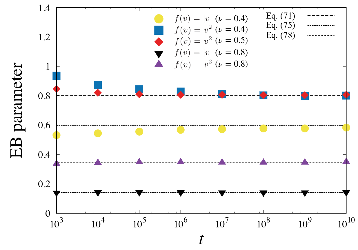
at the critical velocity because we assume .
IV.2 Another derivation of Eq. (21)
Here, we give another derivation of the propagator, i.e., Eq. (21). The joint PDF of with satisfying , denoted by , can be written as
| (25) |
where if the condition in the bracket is satisfied, and 0 otherwise. It follows that the propagator can be obtained as a sum over the number of renewals :
| (26) |
Using and , we have
| (27) |
where we note that gives a probability:
| (28) |
The mean of can be written as
| (29) |
where we used identity . Therefore, we have Eq. (21).

V Infinite invariant density in a semi-Markov process
V.1 Infinite invariant density
To proceed with the discussion of Eq. (23), we use Eq. (6) for the flight-duration PDF and consider . The PDF of velocities in an elementary event can be obtained by Eqs. (5) and (16):
| (30) |
For the specific choice for given in Eq. (6) the asymptotic form with yields
| (31) |
First, we give the asymptotic behavior of for . Because the Laplace transform of is given by for , Eqs. (10) and (11) yields the well-known result:
| (32) |
However, for our purposes, we need to go beyond this limit as shown below. The renewal function gives the exact form of the propagator [see Eq. (21)]. There are two regimes in the propagator as seen in Eq. (22). For , or equivalently , the propagator is given by
| (33) |
In this regime the propagator is an increasing function of because is a monotonically increasing function whose asymptotic behavior is given by Eq. (32), whereas the support will shrink because as . For and , implying , the propagator becomes
| (34) |
This is a universal law in the sense that the asymptotic form does not depend on the detailed form of the flight-duration PDF such as scale parameter .
For , or equivalently , the propagator is given through . For and ,
| (35) | |||||
| (36) |
Therefore, the asymptotic behavior of the propagator becomes
| (37) |
which can also be obtained simply by changing in Eq. (20) into except for the proportional constant. Here, one can define a formal steady state using Eq. (37) as follows:
| (38) |
This does not depend on in the long-time limit and is a natural extension of the steady state for , i.e., Eq. (20). In this sense, is a formal steady state of the system. However, is not normalizable and thus it is sometimes called infinite invariant density. Using Eq. (31), the asymptotic form of the infinite density for becomes
| (39) |
We note that the infinite density describes the propagator only for . While in the long-time limit, the propagator for is composed of two parts, i.e., Eqs. (34) and (37). These behaviors are illustrated in Fig. 1, where the support of the propagator is restricted to . In particular, the accumulation at zero velocity for and a trace of the infinite density for are clearly shown. In general, the propagator for is described by the small- behavior of the flight-duration PDF through Eq. (22).
V.2 Scaling function
Rescaling by in the propagator, we find a scaling function. In particular, the rescaled propagator does not depend on time and approaches the scaling function denoted by in the long-time limit ():
| (40) |
where we used Eq. (35) and note that . In the scaling function, the long-time limit is taken in advance. Thus, the scaling function describes only small- behaviors of . In other words, large- behaviors of are not matched with those of while large- behaviors of are matched with small- behaviors of . The scaling function is normalized and continuous at whereas is not continuous at for finite because the jump in the propagator at is given by Eq. (24) and for . As shown in Fig. 2, rescaled propagators at different times coincide with the scaling function for . Note that the scaling function describes the behavior of for in the long-time limit, which does not capture the behavior of for . Large- behaviors of can be described by . Although depends on the details of , the scaling function is not sensitive to all the details except for . In this sense, it is a general result.

V.3 Ensemble averages
The theory of infinite ergodic theory is a theory of observables. This means that we must classify different observables and define the limiting laws with which their respective ensemble averages are obtained in the long time limit. We will soon consider also time averages. Consider the observable . The corresponding ensemble average is given by
| (41) |
If we take the time , we have
| (42) |
where we performed a change of variable and used the scaling function in the first term, and we also used for in the second and third terms. Moreover, we assume that the second and third term in Eq. (41) does not diverge. In what follows, we consider . When is integrable with respect to , i.e., , satisfies the following inequality:
| (43) |
In this case, the leading term of the asymptotic behavior of the ensemble average is given by the first term:
| (44) |
where we used Eq. (40):
| (45) |
Thus, the ensemble average goes to zero and infinity in the long-time limit for and , respectively. On the other hand, when is integrable with respect to , i.e., , where satisfies with for , the second and third terms becomes
| (46) |
Because the relation between and satisfies , the asymptotic behavior of the ensemble average is given by
| (47) |
A structure of Eqs. (44) and (47) is very similar to an ordinary equilibrium averaging in the sense that there is a time-independent average with respect to or on the right hand side, where the choice of or depends on whether the observable is integrable with respect to or . The beauty of infinite ergodic theory is that this can be extended to time averages, which as mentioned will be discussed below.
In the long-time limit, behaves like a delta distribution in the following sense:
| (48) |
Eq. (48) is clearly obtained when is integrable with respect to , i.e., . Even when is not integrable with respect to , Eq. (48) is valid if is integrable with respect to . In fact, the asymptotic behavior of the ensemble average becomes for , as shown above. Therefore, Eq. (48) is valid in this case. When both integrals diverge, Eq. (48) is no longer valid. However, if there exists a positive constant such that for , Eq. (48) is always valid. In the long-time limit, the ensemble average is trivial in the sense that it simply gives the value of the observable at . At this stage, there is no replacement of a “steady state” concept. However, in general, scaling function describes the propagator near while infinite invariant density describes the propagator for including large- behaviors. Therefore, as shown in Eqs. (44) and (47), both the scaling function and the infinite invariant density play an important role for the evaluation of certain ensemble averages at time .
VI Distributional limit theorems
When the system is stationary, a time average approaches a constant in the long-time limit, which implies ergodicity of the system. However, time averages of some observables may not converge to a constant but properly scaled time averages converge in distribution when the system is non-stationary as it is case for . While we focus on regime , the following theorems can be extended to regime .

To obtain the distribution of these time averages, we consider the propagator of the integrals of these observables along a trajectory from to , denoted by , which are piece-wise-linear functions of and can be described by a continuous accumulation process (see Fig. 3) Akimoto et al. 2015. Time average of function is defined by
| (49) |
As specific examples, we will consider time averages of the absolute value of the velocity and the squared velocity, i.e., or . Integrated value can be represented by
| (50) |
The stochastic process of can be characterized by a recursion relation, which is the same as in the derivation of the velocity propagator. Let be the PDF of when a renewal occurs exactly at time , then we have
| (51) |
where and . Here, we assume that function is an even function. We note that we use a deterministic coupling between and , i.e., Eq. (1). The PDF of at time is given by
| (52) |
where
| (53) |
The double-Laplace transform with respect to and yields
| (54) |
where and are the double-Laplace transforms of and given by
| (55) |
and
| (56) |
respectively. Eq. (54) is the exact form of the PDF of in Laplace space.
Before considering a specific form of , we show that there are two different classes of distributional limit theorems of time averages. Expanding in Eq. (55), we have
| (57) |
Using Eq. (30), one can write the second term with as
| (58) |
When is integrable with respect to the infinite invariant density, i.e., , the second term is still finite for . As shown below, we will see that the integrability gives a condition that determines the shape of the distribution function for the normalized time average, i.e., .
VI.1 Time average of the absolute value of
In this section, we show that there are two phases for distributional behaviors of time averages. The phase line is determined by a relation between and . As a specific choice of function , we consider the absolute value of the velocity, i.e., . Thus, is given by
| (59) |
For , the moment is finite, i.e., . This condition is equivalent to the following condition represented by the infinite density:
| (60) |
The double Laplace transform is calculated in Appendix C (see Eq. (95)). For , the leading term of becomes
| (61) |
It follows that the mean of for becomes
| (62) |
Since the mean of increases with , we consider a situation where for small in the double-Laplace space. Thus, all the term () and in Eq. (95) can be ignored. It follows that the asymptotic form of is given by
| (63) |
This is the double Laplace transform of PDF Feller 1971, where
| (64) |
and is a one sided Lévy distribution; i.e., the Laplace transform of PDF is given by . By a straightforward calculation one obtain the asymptotic behavior of the second moment as follows:
| (65) |
Furthermore, the th moment can be represented by
| (66) |
for . It follows that random variable converges in distribution to a random variable whose PDF follows the Mittag-Leffler distribution of order , where
| (67) |
In other words, the normalized time averages defined by do not converge to a constant but the PDF converge to a non-trivial distribution (the Mittag-Leffler distribution). In particular, the PDF can be represented through the Lévy distribution:
| (68) |
To quantify trajectory-to-trajectory fluctuations of the time averages, we consider the ergodicity breaking (EB) parameter He et al. 2008 defined by
| (69) |
where implies the average with respect to the initial condition. When the system is ergodic, it goes to zero as . On the other hand, it converges to a non-zero constant when the trajectory-to-trajectory fluctuations are intrinsic. For , the EB parameter becomes
| (70) |
which means that time averages do not converge to a constant but they become a random variable with a non-zero variance. For , the EB parameter actually goes to zero in the long-time limit. Moreover, it also goes to zero as in Eq. (70). We note that the condition (60) is general in a sense that the distribution of time averages of function satisfying the condition (60) follows the Mittag-Leffler distribution, which is the same condition as in infinite ergodic theory Aaronson 1997.
For , diverges and equivalently , which results in a distinct behavior of the time averages. Using Eq. (97), we have
| (71) |
for . The inverse Laplace transform gives
| (72) |
for . Therefore, scales as , which means that all the terms of in Eq. (96) cannot be ignored. These terms give the higher order moments. Performing the inverse Laplace transform of terms proportional to gives
| (73) |
for . By Eq. (99), the EB parameter becomes
| (74) |
This EB parameter depends on as well as () and was found also in Ref. Albers 2016. We note that is a decreasing function of . Therefore, trajectory-to-trajectory fluctuations of the time averages becomes insignificant for large . In particular, converges to and 0 for and , respectively. In other words, the system becomes ergodic in the sense that the time averages converge to a constant in the limit of (and ).
VI.2 Time average of the squared velocity
For , can be represented by
| (75) |
By the same calculation as in the previous case, using and , one can express the double Laplace transform of as
| (76) |
Therefore, the limit distribution of can be obtained in the same way as for the previous observable. In particular, the Mittag-Leffler distribution is a universal distribution of the normalized time average of if , i.e., is integrable with respect to the infinite invariant density. On the other hand, the distribution of normalized time averages becomes another distribution for if (see Appendix. C). It follows that for and the EB parameter becomes
| (77) |
This expression was also obtained in Ref. Albers 2016. The exponent in Eq. (77) is different from that found in the EB parameter for with . Therefore, our distributional limit theorem is not universal but depends on the observable. On the other hand, the exponent in the EB parameter for is the same as that for with .
Figure 4 shows that our theory works very well for both observables. For with and (), both of which satisfy , the EB parameters do not depend on . Moreover, Fig. 4 shows that the EB parameter given by is a decreasing function of for .
VII conclusion
We investigated the propagator in an SMP and provided its exact form, which is described by the mean number of renewals [see Eq. (23)]. We assumed that and that this function has support on zero velocity. More specifically, the relation implies that long flight durations favor velocity close to zero since and this is the reason for an accumulation of probability in the vicinity of zero velocity in this model. We prove that the propagator accumulates in the vicinity of zero velocity in the long-time limit when the mean flight-duration diverges () and the coupling parameter fulfills . Taking a closer look at the vicinity of , we found universal behaviors in the asymptotic forms of the propagator. In particular the asymptotic behavior of the propagator for follows two scaling laws, i.e., the infinite invariant density Eq. (38) and the scaling function Eq. (40). The scaling function describes a detailed structure of the propagator near including zero velocity while the infinite invariant density describes the propagator outside . Clearly when , and interestingly the asymptotic form outside becomes a universal form that is unbounded at the origin and cannot be normalized, i.e., an infinite invariant density. One advantage of considering the topic with an SMP is that we can attain an explicit expression for the infinite invariant density Eq. (38). In contrast in general it is hard to find exact infinite invariant measures in deterministic dynamical systems, for example in the context of the Pomeau-Manniville map Manneville and Pomeau 1979; *pomeau1980; *Manneville1980.
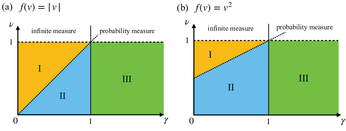
Further, while the Mittag-Leffler distribution describing the distribution of time averages of integrable observables is well known, from the Aaronson-Darling-Kac theorem, we considered here also another distributional limit theorem [see Eqs. (74) and (77)] which describes the distribution of time averages of certain non-integrable observables. Therefore, the integrability of the observable with respect to the infinite invariant density establishes a criterion on the type of distributional limit law, which is similar to findings in infinite ergodic theory. These results will pave the way for constructing physics of non-stationary processes. Finally, we summarize our results by the phase diagram shown in Fig. 5. The infinite invariant density is always observed for . On the other hand, the boundary of the regions I and II depends on the observation function .
Acknowledgement
This work was supported by JSPS KAKENHI Grant Number 16KT0021, 18K03468 (TA). EB thanks the Israel Science Foundation and Humboldt Foundation for support.

Appendix A Exact form of the propagator outside
Here, we consider a specific form for the flight-duration PDF to obtain the exact form of the propagator outside . As a specific form, we use
| (78) |
where is the Mittag-Leffler function with parameter defined as Gorenflo and Mainardi 2008
| (79) |
In fact, the asymptotic behavior is given by a power law Gorenflo and Mainardi 2008, i.e.,
| (80) |
Moreover, it is known that the Laplace transform of is given by
| (81) |
Therefore, the Laplace transform of becomes
| (82) |
and its inverse Laplace transform yields
| (83) |
for any . For , is given by
| (84) |
It follows that the propagator outside becomes
| (85) |
for and . As shown in Fig. 6, the propagator outside is described by Eq. (85), whereas we did not use Eq. (78).
Appendix B another proof of the asymptotic behavior of the propagator of
To obtain the propagator, i.e., the PDF of velocity at time , it is almost equivalent to have the PDF of time interval straddling , i.e., , where is the number of renewals until (not counting the one at ). In ordinary renewal processes, the double Laplace transform of the PDF with respect to and is given by Barkai et al. 2014
| (86) |
For , the asymptotic behavior of this inverse Laplace transform can be calculated using a technique from Ref. Godrèche and Luck 2001. For and ,
| (87) |
This is the asymptotic result, which does not depend on the details of the flight-duration PDF, i.e. different flight-duration PDFs give the same result if the power-law exponent is the same. On the other hand, detail forms of , e.g., the behavior for small and , depend on details of the flight-duration PDF Wang et al. 2018.
Here, we consider a situation where the relation between the velocity and the flight duration is given by . The PDF of velocity at time , i.e., the propagator, can be represented through the PDF :
| (88) |
Note that is symmetric with respect to . Using Eq. (87) yields
| (89) |
The asymptotic form for becomes
| (90) |
for . Therefore, this is consistent with the propagator we obtained in this paper, Eqs. (34) and (37).
For , the PDF has an equilibrium distribution, i.e., for the PDF is given by
| (91) |
where is the mean flight duration Akimoto and Yamamoto 2016b.
Appendix C the double Laplace transform and the exact form of the second moment of for
Here, we represent the double Laplace transform as an infinite series expansion. Expanding in Eqs. (55) and (56), we have
| (92) |
and
| (93) |
for and , respectively, where . Moreover, we have
| (94) |
for . Using Eq. (54), we have
| (95) | |||||
for and
| (96) | |||||
for .
The coefficient of the term proportional to in Eq. (96) is
| (97) |
Moreover, by considering the coefficient of the term proportional to in Eq. (96), the leading term of the second moment of in the Laplace space () can be represented as
| (98) |
where
| (99) |
It follows that the asymptotic behavior of is given by Eq. (73) with .
Since grows as , one can define as
| (100) |
It follows that the random variable converges in distribution to a random variable which depends on both and . More precisely, one obtains
| (101) |
Therefore, the PDF of the normalized time average defined by converges to a non-trivial distribution that is different from the Mittag-Leffler distribution (see Fig. 7).

References
- Akimoto and Aizawa (2007) T. Akimoto and Y. Aizawa, J Korean Phys. Soc. 50, 254 (2007).
- Korabel and Barkai (2009) N. Korabel and E. Barkai, Phys. Rev. Lett. 102, 050601 (2009).
- Akimoto and Miyaguchi (2010) T. Akimoto and T. Miyaguchi, Phys. Rev. E 82, 030102(R) (2010).
- Akimoto and Barkai (2013) T. Akimoto and E. Barkai, Phys. Rev. E 87, 032915 (2013).
- Meyer and Kantz (2017) P. Meyer and H. Kantz, Phys. Rev. E 96, 022217 (2017).
- Bardou et al. (2002) F. Bardou, J.-P. Bouchaud, A. Aspect, and C. Cohen-Tannoudji, Levy statistics and laser cooling: how rare events bring atoms to rest (Cambridge University Press, 2002).
- Bardou et al. (1994) F. Bardou, J. P. Bouchaud, O. Emile, A. Aspect, and C. Cohen-Tannoudji, Phys. Rev. Lett. 72, 203 (1994).
- Bertin and Bardou (2008) E. Bertin and F. Bardou, Am. J. Phys. , 630 (2008).
- Lutz and Renzoni (2013) E. Lutz and F. Renzoni, Nat. Phys. 9, 615 (2013).
- Rebenshtok et al. (2014) A. Rebenshtok, S. Denisov, P. Hänggi, and E. Barkai, Phys. Rev. Lett. 112, 110601 (2014).
- Holz et al. (2015) P. C. Holz, A. Dechant, and E. Lutz, Europhys. Lett. 109, 23001 (2015).
- Leibovich and Barkai (2019) N. Leibovich and E. Barkai, Phys. Rev. E 99, 042138 (2019).
- Wang et al. (2019) X. Wang, W. Deng, and Y. Chen, J. Chem. Phys. 150, 164121 (2019).
- Vezzani et al. (2019) A. Vezzani, E. Barkai, and R. Burioni, Phys. Rev. E 100, 012108 (2019).
- Wang et al. (2018) W. Wang, J. H. P. Schulz, W. Deng, and E. Barkai, Phys. Rev. E 98, 042139 (2018).
- Aghion et al. (2019) E. Aghion, D. A. Kessler, and E. Barkai, Phys. Rev. Lett. 122, 010601 (2019).
- Manneville and Pomeau (1979) P. Manneville and Y. Pomeau, Phys. Lett. A 75, 1 (1979).
- Pomeau and Manneville (1980) Y. Pomeau and P. Manneville, Commun. Math. Phys. 74, 189 (1980).
- Manneville (1980) P. Manneville, J. Phys. (Paris) 41, 1235 (1980).
- Thaler (1983) M. Thaler, Isr. J. Math. 46, 67 (1983).
- Aizawa and Kohyama (1984) Y. Aizawa and T. Kohyama, Prog. Theor. Phys. 71, 847 (1984).
- Aizawa (1984) Y. Aizawa, Prog. Theor. Phys. 72, 659 (1984).
- Aizawa (1989) Y. Aizawa, Prog. Theor. Phys. Suppl. 99, 149 (1989).
- Thaler (1995) M. Thaler, Isr. J. Math. 91, 111 (1995).
- Aaronson (1997) J. Aaronson, An Introduction to Infinite Ergodic Theory (American Mathematical Society, Providence, 1997).
- Thaler (2000) M. Thaler, Studia Math 143, 103 (2000).
- Zweimüller (2004) R. Zweimüller, Fund. Math. 181, 1 (2004).
- Darling and Kac (1957) D. A. Darling and M. Kac, Trans. Am. Math. Soc. 84, 444 (1957).
- Lamperti (1958) J. Lamperti, Trans. Am. Math. Soc. 88, 380 (1958).
- Aaronson (1981) J. Aaronson, J. D’Analyse Math. 39, 203 (1981).
- Thaler (1998) M. Thaler, Trans. Am. Math. Soc. 350, 4593 (1998).
- Thaler (2002) M. Thaler, Ergod. Theory Dyn. Syst. 22, 1289 (2002).
- Thaler and Zweimüller (2006) M. Thaler and R. Zweimüller, Probab. Theory Relat. Fields 135, 15 (2006).
- Akimoto (2008) T. Akimoto, J. Stat. Phys. 132, 171 (2008).
- Akimoto et al. (2015) T. Akimoto, S. Shinkai, and Y. Aizawa, J. Stat. Phys. 158, 476 (2015).
- Korabel and Barkai (2012) N. Korabel and E. Barkai, Phys. Rev. Lett. 108, 060604 (2012).
- Korabel and Barkai (2013) N. Korabel and E. Barkai, Phys. Rev. E 88, 032114 (2013).
- Akimoto and Aizawa (2010) T. Akimoto and Y. Aizawa, Chaos 20, 033110 (2010).
- Akimoto (2012) T. Akimoto, Phys. Rev. Lett. 108, 164101 (2012).
- Meyer et al. (2017) P. Meyer, E. Barkai, and H. Kantz, Phys. Rev. E 96, 062122 (2017).
- Brokmann et al. (2003) X. Brokmann, J.-P. Hermier, G. Messin, P. Desbiolles, J.-P. Bouchaud, and M. Dahan, Phys. Rev. Lett. 90, 120601 (2003).
- Stefani et al. (2009) F. D. Stefani, J. P. Hoogenboom, and E. Barkai, Phys. today 62, 34 (2009).
- Golding and Cox (2006) I. Golding and E. C. Cox, Phys. Rev. Lett. 96, 098102 (2006).
- Weigel et al. (2011) A. Weigel, B. Simon, M. Tamkun, and D. Krapf, Proc. Natl. Acad. Sci. USA 108, 6438 (2011).
- Jeon et al. (2011) J.-H. Jeon, V. Tejedor, S. Burov, E. Barkai, C. Selhuber-Unkel, K. Berg-Sørensen, L. Oddershede, and R. Metzler, Phys. Rev. Lett. 106, 048103 (2011).
- Manzo et al. (2015) C. Manzo, J. A. Torreno-Pina, P. Massignan, G. J. Lapeyre Jr, M. Lewenstein, and M. F. G. Parajo, Phys. Rev. X 5, 011021 (2015).
- Takeuchi and Akimoto (2016) K. A. Takeuchi and T. Akimoto, J. Stat. Phys. 164, 1167 (2016).
- Godrèche and Luck (2001) C. Godrèche and J. M. Luck, J. Stat. Phys. 104, 489 (2001).
- He et al. (2008) Y. He, S. Burov, R. Metzler, and E. Barkai, Phys. Rev. Lett. 101, 058101 (2008).
- Miyaguchi and Akimoto (2011) T. Miyaguchi and T. Akimoto, Phys. Rev. E 83, 031926 (2011).
- Miyaguchi and Akimoto (2013) T. Miyaguchi and T. Akimoto, Phys. Rev. E 87, 032130 (2013).
- Akimoto and Miyaguchi (2013) T. Akimoto and T. Miyaguchi, Phys. Rev. E 87, 062134 (2013).
- Miyaguchi and Akimoto (2015) T. Miyaguchi and T. Akimoto, Phys. Rev. E 91, 010102 (2015).
- Metzler et al. (2014) R. Metzler, J.-H. Jeon, A. G. Cherstvy, and E. Barkai, Phys. Chem. Chem. Phys. 16, 24128 (2014).
- Budini (2016) A. A. Budini, Phys. Rev. E 94, 052142 (2016).
- Budini (2017) A. A. Budini, Phys. Rev. E 95, 052110 (2017).
- Akimoto and Yamamoto (2016a) T. Akimoto and E. Yamamoto, Phys. Rev. E 93, 062109 (2016a).
- Akimoto and Yamamoto (2016b) T. Akimoto and E. Yamamoto, J. Stat. Mech. 2016, 123201 (2016b).
- Akimoto et al. (2016) T. Akimoto, E. Barkai, and K. Saito, Phys. Rev. Lett. 117, 180602 (2016).
- Akimoto et al. (2018a) T. Akimoto, E. Barkai, and K. Saito, Phys. Rev. E 97, 052143 (2018a).
- Albers and Radons (2014) T. Albers and G. Radons, Phys. Rev. Lett. 113, 184101 (2014).
- Albers (2016) T. Albers, PhD Thesis, Technischen Universität Chemnitz,Chemnitz (2016).
- Albers and Radons (2018) T. Albers and G. Radons, Phys. Rev. Lett. 120, 104501 (2018).
- Shlesinger et al. (1987) M. F. Shlesinger, B. J. West, and J. Klafter, Phys. Rev. Lett. 58, 1100 (1987).
- Karatzas and Shreve (2012) I. Karatzas and S. Shreve, Brownian motion and stochastic calculus, Vol. 113 (Springer Science & Business Media, 2012).
- Cox (1962) D. R. Cox, Renewal theory (Methuen, London, 1962).
- Metzler and Klafter (2000) R. Metzler and J. Klafter, Phys. Rep. 339, 1 (2000).
- Helmstetter and Sornette (2002) A. Helmstetter and D. Sornette, Phys. Rev. E 66, 061104 (2002).
- Bouchaud and Georges (1990) J. Bouchaud and A. Georges, Phys. Rep. 195, 127 (1990).
- Meyer et al. (2018) P. G. Meyer, V. Adlakha, H. Kantz, and K. E. Bassler, New J. Phys. 20, 113033 (2018).
- Richardson (1926) L. F. Richardson, Proc. R. Soc. A. 110, 709 (1926).
- Obukhov (1959) A. Obukhov, Adv. Geophys., 6, 113 (1959).
- Aghion et al. (2018) E. Aghion, D. A. Kessler, and E. Barkai, Eur. Phys. J. B 91, 17 (2018).
- Bothe et al. (2019) M. Bothe, F. Sagues, and I. M. Sokolov, Phys. Rev. E 100, 012117 (2019).
- Klafter et al. (1987) J. Klafter, A. Blumen, and M. F. Shlesinger, Phys. Rev. A 35, 3081 (1987).
- Barkai et al. (2014) E. Barkai, E. Aghion, and D. A. Kessler, Phys. Rev. X 4, 021036 (2014).
- Montroll and Weiss (1965) E. W. Montroll and G. H. Weiss, J. Math. Phys. 6, 167 (1965).
- Akimoto and Miyaguchi (2014) T. Akimoto and T. Miyaguchi, J. Stat. Phys. 157, 515 (2014).
- Miyaguchi et al. (2016) T. Miyaguchi, T. Akimoto, and E. Yamamoto, Phys. Rev. E 94, 012109 (2016).
- Akimoto et al. (2018b) T. Akimoto, A. G. Cherstvy, and R. Metzler, Phys. Rev. E 98, 022105 (2018b).
- Feller (1971) W. Feller, An Introduction to Probability Theory and its Applications, 2nd ed., Vol. 2 (Wiley, New York, 1971).
- Gorenflo and Mainardi (2008) R. Gorenflo and F. Mainardi, Anomalous Transport: Foundations and Applications 4, 93 (2008).