Switch-based Hybrid Beamforming for Massive MIMO Communications in mmWave Bands

Massive multiple-input multiple-output (MIMO) systems in millimetre wave (mmWave) bands are promising candidates for future generation wireless cellular communications systems to alleviate spectrum congestion and bandwidth scarcity [1]. Communications in mmWave band, which makes use of frequency bands from 30 to 300 GHz, is an enabling technology for fifth-generation (5G) networks. The smaller wavelengths in mmWave communications systems make large-scale antenna arrays at the transceivers viable. This leads to various new challenges for fully-digital beamforming in mmWave massive MIMO systems, such as prohibitively high hardware complexity, computational cost and power consumption [2, 3, 4].

Digital processing for traditional MIMO communications systems requires that each array element has a dedicated RF and baseband hardware chains comprising expensive components [5]. Thus, full digital processing is undesirable and impractical due to the cost and complexity of the hardware chains in mmWave MIMO communications systems with large arrays [6, 7]. Furthermore, components such as RF up/down converters and analog-to-digital converters (ADCs) (or digital-to-analog converters (DACs)) are not only expensive but also have high power consumption [8]. This motivates various strategies for the efficient implementation of beamforming for massive MIMO systems in mmWave bands, including hybrid beamforming architectures [9, 10, 11, 12, 13, 14, 15, 4, 8, 1], beamspace signal processing techniques [16, 17], lens-based analog beamforming antennas [18], and low-rate ADC methods [19].

Hybrid beamforming for massive MIMO communications systems has been extensively studied in recent years, see [20] and the references therein. It is a well-established approach that employs a two-stage analog and digital processing configuration. The analog precoding stage employs simpler and less power-hungry analog beamformers to present a reduced-dimensional signal to the baseband stage [21]. Typically, the analog precoding stage is implemented as a network of phase shifters [22]. While this achieves a level of simplification over fully digital RF chains, the practical realization of the phase shifters for mmWave frequencies is not a simple task [23]. MmWave digitally controlled phase shifters have finite precision that may not be sufficient to form the desired beams [23], and their latency may lead to performance degradation if the channel is rapidly changing [20]. Their phase precision can be improved but at the cost of higher power consumption [24]. Passive phase shifters, on the other hand, can alleviate the power consumption problem, but they are known to incur higher losses, requiring additional amplification to maintain an acceptable output signal-to-noise ratio (SNR) [23].

The challenges associated with the use of phase shifters have motivated research into alternative approaches for the realization of the analog precoder. In particular, switch-based networks are simple, low-power and high-speed solutions to these challenges [20, 22]. These switch-based combiners effectively combine subsets of the available antennas such that they are able to leverage the sparse nature of mmWave massive MIMO channels to realize performance gains [24]. In fact, different realizations and special cases of the switch-based approach have been successfully applied in various contexts. For instance, optimal selection of a subset of “best” antennas from a larger set of antennas has been shown as a promising approach for delivering a large aperture with satisfactory performance at reduced hardware cost and complexity [25, 26, 27, 28, 29, 30]. When the complexity of connectivity, routing, and RF multiplexing are of grave concern, the switching network can be partitioned into subsets, and only a few antennas per subset are then selected [22, 31, 32].

The solution to the hybrid beamforming problem is not straightforward, and replacing the phase shifters with simple switches greatly exacerbates the difficulty of this task as optimization over a set of binary variables is then required. A dictionary-based strategy was proposed in [33] to address this, but the dictionary grows exponentially with the number of antennas, making this method impractical for large antenna arrays. Furthermore, as this dictionary is scenario-specific, it must be redesigned for every problem variation, which adds another layer of complexity to it. In [21] a unified greedy algorithm is proposed for the design of both phase-shifter and switch-based networks. However, the proposed greedy algorithm is limited to the case where the digital beamforming matrix is square with a dimension equal to the number of data streams to be transmitted. Moreover, the proposed greedy method is only suitable for the design of an unconstrained switch-based hybrid beamformer, as its formulation prevents the incorporation of any specific constraints.

Thus, here we propose a novel approach that has the capability of solving a switch-based hybrid beamformer design problem for massive MIMO communications in mmWave bands, which also has the flexibility to include a variety of desirable constraints. To this end, we formulate the problem as an optimization. We decouple the transmit and receive problems, and decompose the joint optimization of the analog and digital precoder matrices into a rank-constrained single variable problem. Then we proceed to solve this problem via two different strategies. In the first method, by approximating the mutual information via a Frobenius norm, we are able to cast the problem as a norm maximization. We then proceed to solve the non-convex maximization via a sequence of optimizations in a modified version of sequential convex programming (SCP). In order to address the mismatch between the norm maximization and the mutual information maximization, the SCP is guided by the actual value of mutual information in each step. In the second method, so as to reduce computational complexity, we take advantage of a lower bound given by QR factorization and iteratively optimize the columns of the analog precoder such that in each iteration we maximize a quadratic form via a SCP.

Hence, the contributions of this paper are:

• •

  We propose a method to solve the problem of switch-based hybrid beamforming for massive MIMO communications in mmWave bands based on convex optimization. This formulation allows for the examination of several cases with various practical limitations on hardware resources.

• •

  As the vast majority of hybrid design methods are based on the assumption that the optimal beamformer is realized by a combination of digital and analog beamformers, there is a mismatch between the approximated solution and the exact one. To address this issue, which is more extreme in a switch-based network due to the binary nature of the variables and the corresponding feasible solution space, we propose a heuristic method based on Gaussian randomization.

• •

  We propose two cost functions as surrogates for the maximization of the mutual information based on (1) a Frobenius norm approximation, and (2) a QR lower bound.

• •

  We study partially connected switch-based networks and propose a method to model specific requirements, imposed by an arbitrary partially connected network, using linear constraints.

A hybrid structure for a single-user mmWave MIMO system is depicted in Fig. 1. In this setup, the transmitter comprises $N_{\mathrm{t}}$ antennas and $k_{\mathrm{t}}$ RF transmit chains, and is required to send $N_{\mathrm{s}}$ data streams to the receiver. We assume that $N_{\mathrm{s}}\leq k_{\mathrm{t}}\leq N_{\mathrm{t}}$. Let the transmit digital beamforming matrix be $\textbf{F}_{\mathrm{BB}}$ of size $k_{\mathrm{t}}\times N_{\mathrm{s}}$, and RF precoder matrix be $\textbf{F}_{\mathrm{RF}}$ of size $N_{\mathrm{t}}\times k_{\mathrm{t}}$. $\textbf{F}_{\mathrm{RF}}$ is implemented using analog phase-shifters or RF switches. The discrete-time transmit signal is then $\textbf{x}=\textbf{F}\textbf{s}$, where $\textbf{F}=\textbf{F}_{\mathrm{RF}}\textbf{F}_{\mathrm{BB}}$, and s is the $N_{\mathrm{s}}\times 1$ symbol vector such that $\mathbb{E}[\textbf{s}\textbf{s}^{H}]=\frac{1}{N_{\mathrm{s}}}\textbf{I}_{N_{\mathrm{s}}}$ with $\mathbb{E}$ denoting the expected value. At the receiver, $N_{\mathrm{r}}$ antennas are connected to $k_{\mathrm{r}}$ RF receive chains to recover the transmitted symbol s. Similarly to the transmitter, the receive beamformer $\textbf{W}=\textbf{W}_{\mathrm{RF}}\textbf{W}_{\mathrm{BB}}$ is composed of the $N_{\mathrm{r}}\times k_{\mathrm{r}}$ RF combining matrix $\textbf{W}_{\mathrm{RF}}$ and $k_{\mathrm{r}}\times N_{\mathrm{s}}$ baseband beamforming matrix $\textbf{W}_{\mathrm{BB}}$.

Given a narrowband frequency-flat channel model represented by the $N_{\mathrm{r}}\times N_{\mathrm{t}}$ channel matrix H, with $\mathbb{E}\left[\|\textbf{H}\|_{F}^{2}\right]=N_{\mathrm{t}}\times N_{\mathrm{r}}$, we can write the received signal as

Here $\rho$ is the average received power, and n the additive zero-mean i.i.d noise with variance $\sigma_{n}^{2}$. Also, $\textbf{W}_{\mathrm{BB}}^{H}$ denotes the conjugate transpose of $\textbf{W}_{\mathrm{BB}}$. For a clustered channel model consisting of the sum of the contributions of $N_{\mathrm{cl}}$ scattering clusters, with each cluster comprising $N_{\mathrm{ray}}$ propagation paths, the channel matrix is

where $\gamma=\sqrt{\frac{N_{\mathrm{rt}}N_{\mathrm{r}}}{N_{\mathrm{cl}}N_{\mathrm{ray}}}}$ is a normalization factor and $\alpha_{i\ell}$ is the complex amplitude associated with the $\ell$-th ray in the $i$-th cluster. The antenna gain at the direction of departure (DoD) azimuth and elevation angles $(\phi_{i\ell}^{\mathrm{t}},\theta_{i\ell}^{\mathrm{t}})$, and the direction of arrival (DoA)$(\phi_{i\ell}^{\mathrm{r}},\theta_{i\ell}^{\mathrm{r}})$, are denoted by $\Lambda_{\mathrm{r}}(\phi_{i\ell}^{\mathrm{r}},\theta_{i\ell}^{\mathrm{r}})$, and $\Lambda_{\mathrm{t}}(\phi_{i\ell}^{\mathrm{r}},\theta_{i\ell}^{\mathrm{r}})$ respectively. The DoDs and DoAs of the scatterers are assumed randomly distributed with a Laplacian distribution [4]. The vectors, $\textbf{a}_{\mathrm{r}}(\phi_{i\ell}^{\mathrm{r}},\theta_{i\ell}^{\mathrm{r}})$ and $\textbf{a}_{\mathrm{t}}(\phi_{i\ell}^{\mathrm{r}},\theta_{i\ell}^{\mathrm{r}})$ are respectively the receive and transmit array steering vectors associated with the $\ell$-th ray in the $i$-th cluster. For an uniform planar array (UPA) located in the $yz$-plane, the array response is

where $N$ is the total number of elements, while $N_{y}$ and $N_{z}$ are the number of grid points in the $y$, and $z$ planes respectively such that $N=N_{y}N_{z}$.

Let the transmit power be divided equally among all the data streams. Then, the mutual information is expressed as

Here, $\textbf{R}_{n}$ is the noise covariance matrix at the receiver given by $\textbf{R}_{n}=\sigma^{2}\textbf{W}_{\mathrm{BB}}^{H}\textbf{W}_{\mathrm{RF}}^{H}\textbf{W}_{\mathrm{RF}}\textbf{W}_{\mathrm{BB}}$. The optimum beamformer is composed of the precoding and combining matrices ($\textbf{F}_{\mathrm{BB}},\textbf{F}_{\mathrm{RF}},\textbf{W}_{\mathrm{BB}},\textbf{W}_{\mathrm{RF}}$) that maximize the mutual information. However, this design problem is a joint non-convex optimization that is intractable. To overcome this difficulty, we decompose it into separate transmit and receive subproblems [4], which yields the mutual information at the transmit-side

Furthermore, by defining a virtual channel for the receive section as $\textbf{H}_{\mathrm{r}}=\textbf{H}\textbf{F}_{\mathrm{opt}}$ with $\textbf{F}_{\mathrm{opt}}$ being the optimum precoder employed at the transmit side, the mutual information at the receive-side can be specified as

Hence, the problem is transformed to enable the separate design of precoding and combining matrices.

In general, the analog precoder and combining matrices, $\textbf{F}_{\mathrm{RF}}$ and $\textbf{W}_{\mathrm{RF}}$, are implemented either using analog phase shifters or analog switches along with RF combiners/splitters. In this paper, we focus on hybrid architectures based on switch networks and consider only the transmit-side.

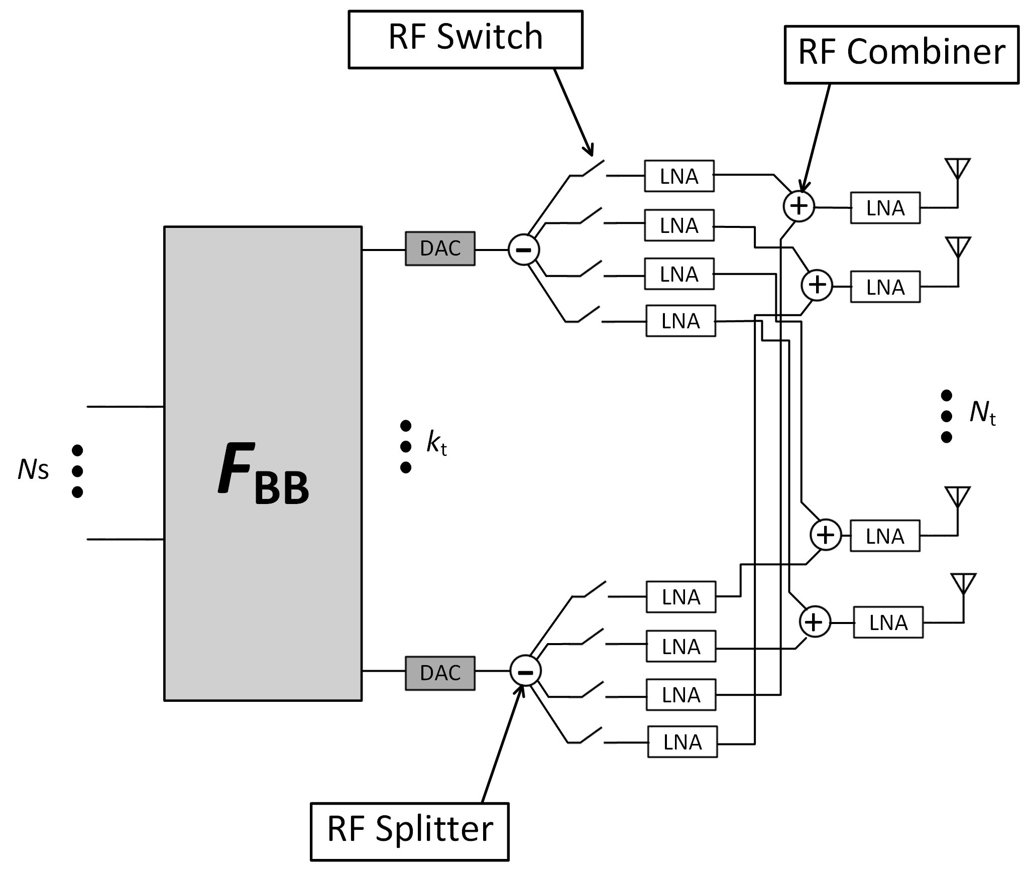
Given a hybrid precoder based on a network of analog switches, we sketch the general model for splitting, switching, and combining in Fig. 2. The $N_{\mathrm{s}}$ data streams are first digitally precoded by $\textbf{F}_{\mathrm{BB}}$. Then each of ${k_{\mathrm{t}}}$ precoded signals is converted into the RF domain through a DAC. The RF signal is then split into $N_{\mathrm{t}}$ branches, and each split signal is directed to a low-noise amplifier (LNA) via an RF switch. Finally, in each transmit antenna, a set of ${k_{\mathrm{t}}}$ signals are combined, amplified and transmitted.

We begin the design by finding the optimum precoding matrix. Given that the channel has a singular value decomposition, e.g., ${\textbf{H}}=\textbf{U}\boldsymbol{\Sigma}\textbf{V}^{H}$ such that U is an $N_{\mathrm{r}}\times\mathrm{rank}({\textbf{H}})$ unitary matrix, $\boldsymbol{\Sigma}$ is a $\mathrm{rank}({\textbf{H}})\times\mathrm{rank}({\textbf{H}})$ diagonal matrix of descending singular values, and is a unitary matrix. The unconstrained optimum precoder is given by the first $N_{\mathrm{s}}$ singular vectors and the diagonal matrix $\Gamma$ as $\textbf{F}_{\mathrm{opt}}=\textbf{V}_{N_{\mathrm{s}}}\boldsymbol{\Gamma}$. The diagonal matrix $\Gamma$ is effectively obtained via a water-filling power allocation method. Hence, it is reasonable to split the optimum precoder, consider an equal power allocation ($\boldsymbol{\Gamma}=\textbf{I}$), and apply the power allocation matrix when required. By employing the unconstrained optimum precoder, we have

We assume that the mmWave system and propagation channel parameters are selected such that a hybrid precoder $\textbf{F}_{\mathrm{RF}}\textbf{F}_{\mathrm{BB}}$, sufficiently close to $\textbf{F}_{\mathrm{opt}}=\textbf{V}_{N_{\mathrm{s}}}$, is attainable. Thus, it is assumed that the matrices $\textbf{I}_{N_{\mathrm{s}}}-\textbf{V}_{N_{\mathrm{s}}}^{H}\textbf{F}_{\mathrm{RF}}\textbf{F}_{\mathrm{BB}}\textbf{F}_{\mathrm{BB}}^{H}\textbf{F}_{\mathrm{RF}}\textbf{V}_{N_{\mathrm{s}}}$, and $\textbf{V}_{\bar{N}_{\mathrm{s}}}^{H}\textbf{F}_{\mathrm{RF}}\textbf{F}_{\mathrm{BB}}$ have a set of sufficiently small eigenvalues [4]. Note that $\textbf{V}_{\bar{N}_{\mathrm{s}}}$ denotes the eigenvectors associated with the subspace complementary to $\textbf{V}_{{N}_{\mathrm{s}}}$. Now by employing Sylvester’s determinant theorem, and Schur’s complement identity for matrix determinants, we can specify the mutual information as

where $\textbf{H}_{1}$ is the channel constructed by the first $N_{\mathrm{s}}$ singular vectors and singular values of H.

If we define a new virtual matrix $\tilde{\textbf{H}}=\textbf{H}_{1}\textbf{F}_{\mathrm{RF}}$ of size $N_{\mathrm{r}}\times{k_{\mathrm{t}}}$ and singular value decomposition of $\tilde{\textbf{H}}=\tilde{\textbf{U}}\tilde{\boldsymbol{\Sigma}}\tilde{\textbf{V}}^{H}$, we can maximize (6) by having $\textbf{F}_{\mathrm{BB}}=\tilde{\textbf{V}}_{N_{\mathrm{s}}}$.

where $\tilde{\textbf{H}}_{1}$ denotes the new virtual channel representation achieved by the first $N_{\mathrm{s}}$ eigenvalues, e.g., $\tilde{\textbf{H}}_{1}=\tilde{\textbf{U}}_{N_{\mathrm{s}}}\tilde{\textbf{S}}_{N_{\mathrm{s}}}\tilde{\textbf{V}}_{N_{\mathrm{s}}}^{H}$. Note that here $\textbf{F}_{\mathrm{BB}}=\tilde{\textbf{V}}_{N_{\mathrm{s}}}$ can be exactly achieved as we have only a digital beamformer. Now, if we assume that $\mathrm{rank}(\tilde{\textbf{H}})=N_{\mathrm{s}}$, then $\textbf{F}_{\mathrm{BB}}=\tilde{\textbf{V}}_{N_{\mathrm{s}}}=\tilde{\textbf{V}}$ becomes a unitary matrix, and therefore we can write (7) as

Noting that (8) and (6) are equal given that $\mathrm{rank}(\tilde{\textbf{H}})=N_{\mathrm{s}}$ and $\textbf{F}_{\mathrm{BB}}=\tilde{\textbf{V}}_{N_{\mathrm{s}}}$, we can approximate (8) as [4]:

Hence, to maximize (8), we have to maximize $\|\textbf{V}_{1}^{H}\textbf{F}_{\mathrm{RF}}\textbf{F}_{\mathrm{BB}}\|_{F}^{2}$. Furthermore, the rank of $\textbf{F}_{\mathrm{RF}}$ should necessarily be greater than or equal to $N_{s}$ in order to have $\mathrm{rank}(\textbf{H}_{1}\textbf{F}_{\mathrm{RF}})=N_{\mathrm{s}}$. Additionally, $\textbf{V}_{1}^{H}$ is a matrix with $N_{s}$ orthonormal vectors spanning the space of $\tilde{\textbf{H}}$. Thus, the product $\textbf{P}=\textbf{V}_{1}^{H}\textbf{F}_{\mathrm{RF}}$ must have rank $N_{\mathrm{s}}$ and must span the space of $\tilde{\textbf{H}}$. Note that its columns are not orthonormal, but they form a basis for $\mathrm{span}(\textbf{P})$. As this space is also spanned by $\textbf{F}_{\mathrm{BB}}$, then $\textbf{P}=\textbf{V}_{1}^{H}\textbf{F}_{\mathrm{RF}}\in\mathrm{span}(\textbf{F}_{\mathrm{BB}})$. Therefore, the projection of P onto $\textbf{F}_{\mathrm{BB}}$ does not change its Frobenius norm, giving

The maximization problem can then be cast as,

Although we could reduce the problem of joint design of $\textbf{F}_{\mathrm{RF}}$, and $\textbf{F}_{\mathrm{BB}}$ to that of only optimising $\textbf{F}_{\mathrm{RF}}$, the maximization in (11) is non-convex due to norm maximization, the rank constraint, the binary constraint, the norm equality constraint, and the inherent dependence of $\textbf{F}_{\mathrm{BB}}$ on $\textbf{F}_{\mathrm{RF}}$.

If we relax the rank constraint to $\mathrm{rank}(\textbf{H}_{1}\textbf{F}_{\mathrm{RF}})\leq N_{\mathrm{s}}$, noting that $\textbf{H}_{1}$ is of rank $N_{\mathrm{s}}$, the only condition that we need to meet is that $\mathrm{rank}(\textbf{F}_{\mathrm{RF}})\geq N_{\mathrm{s}}$. There exist some algorithms to constrain the rank, i.e., employing a $\mathrm{Trace}(\cdot)$ function as a surrogate for the rank constraint [34]. However, applying this method requires the introduction of a slack variable that leads to an increase in the dimensionality and, subsequently, a higher computational complexity. Therefore, we lift the rank constraint and devise heuristic approaches to address this restriction.

We deal with the norm equality constraint (11c) in two steps. To alleviate the binary property of the problem and the complexity that the norm equality constraint causes in conjunction with the rank constraint, first, we exclude the baseband precoder $\textbf{F}_{\mathrm{BB}}$ and meet the constraint later by scaling $\textbf{F}_{\mathrm{BB}}$.

Furthermore, after relaxing the binary constraint on $\textbf{F}_{\mathrm{RF}}$, we can reformulate the problem as

Thus far, we have been able to relax the non-convex constraints. However, the maximization of the Frobenius norm function in (12) as a convex function is a non-convex problem. Sequential convex programming (SCP) based on iteratively linearizing the convex function is applied to reformulate the non-convex problem as a series of convex subproblems, each of which can be optimally solved using convex programming [34]. We formulate the norm maximization by linearization and use a first-order Taylor expansion as a local approximation. Given $f(\textbf{F}_{\mathrm{RF}})=\|\textbf{V}_{1}^{H}\textbf{F}_{\mathrm{RF}}\|^{2}_{F}$, we express this approximation at point $\ell-1$ as,

where $\mathrm{vec}(.)$ denotes vectorization, which stacks the matrix column by column. By linearization we transform the Frobenius norm to an affine form to enable the solving of this maximization by SCP. The convex problem to be solved in the $\ell$-th step can be expressed as:

After initiation, the SCP procedure approaches a local optimum of (14) iteratively.

In this section, we propose another method to maximize (8) based on majorization theory. To begin, we propose a lower bound on (8) by the following Theorem.

By solving (12), we design the analog precoding matrices $\textbf{F}_{\mathrm{RF}}$, and $\textbf{F}_{\mathrm{BB}}$ based on a switching network without specific hardware limitations. The proposed formulation allows us to impose arbitrary hardware requirements, a feature that is neither feasible in a greedy method nor viable in dictionary-based techniques.

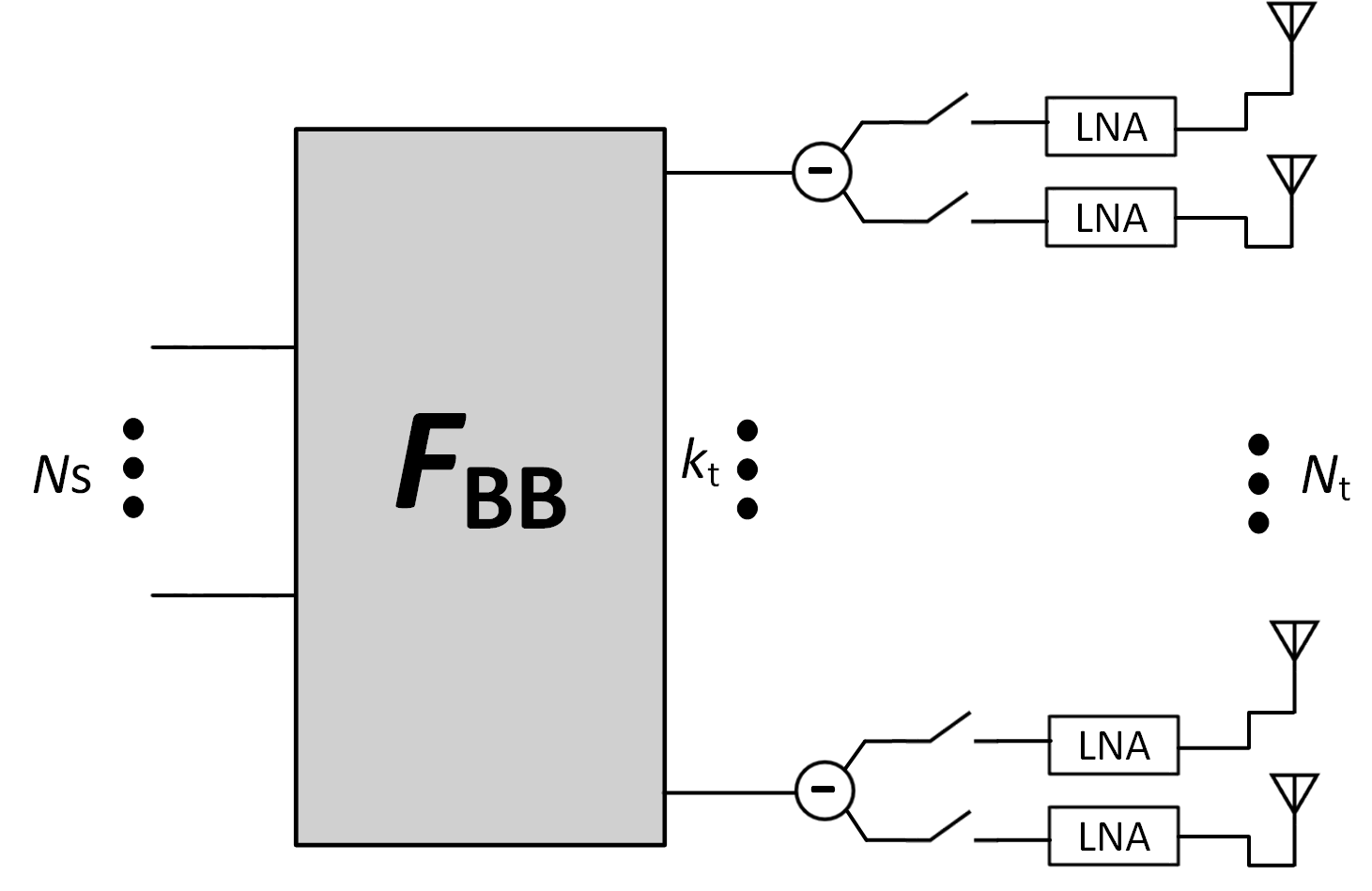
Generally, in a switch-based hybrid precoder and from the structure shown in Fig. 2, we can define hardware limitations in terms of: (1) The number of outputs of the splitters ($s_{\mathrm{t}}$ in Fig. 4); (2) The number of inputs of the analog precoders in each antenna ($c_{\mathrm{t}}$ in Fig. 4); and (3) The predefined connectivity constraint that allows possible connections between the splitters and combiners ($\textbf{G}_{\mathrm{t}}$ in Fig. 4).

The mentioned characteristics are inter-related. If we define the set of antennas that are connected to the $\ell$-th splitter via a binary vector $\textbf{g}_{\mathrm{t},\ell}$, we can then concatenate all the ${k_{\mathrm{t}}}$ vectors in the connectivity matrix $\textbf{G}_{\mathrm{t}}$ as follows,

Given the connectivity matrix, the other two attributes of the switch network must follow as

Furthermore, the total number of connections $n_{G}$ has to follow

Assuming some hardware constraints are imposed by $\textbf{G}_{\mathrm{t}},s_{\mathrm{t}}$, and $c_{\mathrm{t}}$, we can introduce a new subspace to optimize (14), or (25) as

where $\bar{\textbf{g}}_{\mathrm{t},i}$ is the Boolean complement of $\textbf{g}_{\mathrm{t},i}$. Therefore, we can cast the problem of switch-based hybrid design in a partially connected network as,

and we then can solve it via Algorithm 1, or Algorithm 2.

One common scenario for partially connected switch-based hybrid design is to design for an analog precoder, given that there is no analog combiner in the input of antennas ($c_{\mathrm{t}}=1$) as shown in Fig. 5. In this case, $s_{\mathrm{t}}$ is chosen such that ${k_{\mathrm{t}}}s_{\mathrm{t}}=N_{\mathrm{t}}$. Moreover, the connectivity matrix $\textbf{G}_{\mathrm{t}}$ is a set of mutually exclusive columns i.e. $\textbf{g}_{\mathrm{t},i}$.

In this section, we evaluate the performance of the proposed methods through numerical examples. We maximize the spectral efficiency by maximising the mutual information of the transmit side and we assume that there is an ideal combiner at the receiver (i.e. $\textbf{W}=\textbf{I}$). We use a clustered channel model with $N_{\mathrm{cl}}=8$ clusters and $N_{\mathrm{ray}}=10$ rays in each cluster with randomly distributed AoDs, and AoAs sampled from a Laplacian distribution [37]. We also assume that the complex amplitudes of the rays are sampled from a complex normal distribution with an average power of unity in each cluster. The system model that we adopt is a switch-based hybrid beamformer with $N_{\mathrm{t}}=64$ antennas and ${k_{\mathrm{t}}}=4$ RF chains at the transmit side, and with $N_{\mathrm{r}}=16$ antennas and ${k_{\mathrm{t}}}=4$ RF chains at the receive side. The transmit and receive antenna arrays are uniform planar arrays (UPA) with an inter-element spacing, $d$, of a half-wavelength. We have assumed a sector azimuth angle of $60^{\circ}$, and sector elevation angle of $30^{\circ}$ on the transmit side, while on the receive side we assume omni-directional antennas [38, 4].

We analyze the performance of the described system for different numbers of data streams, $N_{\mathrm{s}}$. For each scenario, we calculate the unconstrained optimal precoder (UOP) achieved by the first $N_{\mathrm{s}}$ eigenmodes of the channel. Moreover, we compare the performance to a phase shifter network by implementing an algorithm called spatially sparse precoding (SSP) proposed in [4] as a fast method to design a hybrid network with phase shifters in the analog section. It is worth noting that the hybrid precoder matrix achieved by SSP does not necessarily provide an equal power allocation for an arbitrary structure.

In the case of $N_{\mathrm{s}}={k_{\mathrm{t}}}=4$, we implement the greedy algorithm in [21] in switch network mode. We call this algorithm switch-based hybrid design by unified greedy algorithm (SHD-UG). We then design the switch network with the proposed algorithms, Algorithm 1, Switch-based Hybrid Design by norm maximization (SHD-NM), and Algorithm 2 switch-based hybrid design by QR decomposition with quadratic update (SHD-QRQU). We also implement SHD-NM for designing the switch-based precoder in a partially connected network (SHD-NM-PC). We use the following connectivity matrix for this case,

For convenience of reference, Table I lists the methods that we study by numerical examples. We use $L=1000$, and $I=1000$ when running Algorithm 1, unless stated otherwise. The spectral efficiency for each value is the averaged value of 100 random channel realizations. Furthermore, we use the CVX package [39] to solve the convex optimizations in Algorithms 1, and  2.

Fig. 6 shows the spectral efficiency achieved in a $64\times 16$ UPA for different values of SNR. Both transmitter sand receivers are assumed to have access to 4 RF chains (${k_{\mathrm{t}}}={k_{\mathrm{r}}}=4$). Also, it is assumed that $N_{\mathrm{s}}=2$ data streams are transmitted. Fig. 6 illustrates that the proposed method, SHD-NM achieves spectral efficiencies with only a small gap to those achieved by the unconstrained precoder (UOP), and SSP. Considering the significantly lower cost, power, and hardware complexity required by a switch-based hybrid method, such a small gap demonstrates a very good trade-off. Furthermore, the spectral efficiency achieved in a partially connected network sits closely below the fully connected network and introduces yet lower cost, power and complexity. The spectral efficiency attained by SHD-NM for a fully connected network is always superior to that of SHD-QRQU. The same trend holds for partially connected networks as shown by SHD-NM-PC, and SHD-QRQU-PC.

In Fig. 7 we study the performance for the case of transmitting $N_{\mathrm{s}}=3$ data streams. In this scenario, the hybrid network approximates $N_{\mathrm{s}}=3$ eigenmodes of the channel and the gap between the unconstrained precoder and SSP increases. The switch-based hybrid precoder also experiences larger degradation than that of the phase shift-based strategy, which reflects natural limitations of the switch-based method to approximate 3 eigen-channels with only 4 RF chains and a switch network. Moreover, we can observe that by increasing the number of streams, SHD-QRQU-PC gets closer to SHD-NM-PC.

Next, we examine the performance of the proposed method when $N_{\mathrm{s}}=4$ in Fig. 8. This scenario is a special case as it is categorized as a hybrid network with ${k_{\mathrm{t}}}=N_{\mathrm{s}}$. This class of hybrid networks has been studied frequently in literature, e.g. [40, 21, 5]. In this case, the digital precoding matrix $\textbf{F}_{\mathrm{BB}}$ becomes a square matrix, and therefore the unitary structure of $\textbf{F}_{\mathrm{BB}}$ (as opposed to the generally semi-unitary structure) enables us to decouple the joint design of $\textbf{F}_{\mathrm{RF}},\textbf{F}_{\mathrm{BB}}$ and design $\textbf{F}_{\mathrm{RF}}$ as an isolated variable. For this scenario, we compare the performance of SHD-NM and SHD-QRQU as a comprehensive solutions with that of the unified greedy algorithm (SHD-UGD) proposed in [21].

As we expected by increasing $N_{\mathrm{s}}$, the ability of the hybrid network to approximate the optimal unconstrained precoder slightly deteriorates. This can be observed by the increased gap between SSP, and UOP in Fig. 8 when compared to previous cases shown in Figs. 6, 7. Also, the switch-based network generally has a larger gap to the unconstrained and phase shift based hybrid structure. As shown in this figure, the proposed algorithms outperform the greedy method (SHD-UGD). While the SHD-NM algorithm provides significantly better performance compared to SHD-UGD, the SHD-QRQU method performs slightly better than SHD-UGD. Another important trend is that SHD-QRQU-PC exhibits better performance compared to that of SHD-NM-PC. This shows that although in a fully-connected network, SHD-QRQU demonstrates an inferior performance compared to SHD-NM, in a partially-connected network and for certain structures, it can outperform the more computationally expensive SHD-NM.

We next study the effect of the number of data streams for a fixed value of SNR in Fig. 9. In this example, we employ a $64\times 16$ UPA equipped with 12 RF chains at both transmit and receive sides ($k_{\mathrm{t}}=k_{\mathrm{r}}=12$). We fix the SNR at 0 dB and run the algorithms for varying values of data streams, i.e. $N_{\mathrm{s}}=3,...,12$. The spectral efficiency decreases with an increasing number of data streams. It is worth noting that the SSP algorithm not only achieves a performance very close to the optimum precoder (UOP), but also it outperforms UOP at higher values of $N_{\mathrm{s}}$. We can account for this by noting that the SSP algorithm does not necessarily provide a precoder with equal power allocation. Hence, SSP can outperform the UOP with an unequal power allocation, which is not desirable.

The proposed algorithms, SHD-NM and SHD-QRQU, show a reasonable performance by tracking the optimum precoder and maintaining a consistent gap to this optimum. As we observed in Figs. 6, 7,  and 8, the SHD-QRQU, gets closer to SHD-NM with increasing $N_{\mathrm{s}}$. It should be noted that we have developed SHD-QRQU based on a QR factorization for a square matrix of an analog precoder. For non-square cases we approximate an invertible $(\textbf{H}_{1}\textbf{F}_{\mathrm{RF}}^{i})$ in each step to be able to compute $\textbf{A}_{i}$. As $N_{\mathrm{s}}$ gets closer to $k_{\mathrm{t}}$, the analog precoder gets closer to a square matrix, and it leads to better performance. Moreover, the feasible solution space shrinks by increasing the number of data streams as the digital beamformer consumes more DoFs provided by the virtual eigen-channels (including the analog precoder and the channel). In this case, the capability of SHD-NM deteriorates since it searches a smaller space for modifying the direction. The boosted performance of SHD-QRQU algorithm for a square analog precoder matrix is confirmed in partially connected networks. The SHD-NM-PC achieves higher spectral efficiency in lower values of $N_{\mathrm{s}}$, i.e. $N_{\mathrm{s}}\leq 8$. However, the spectral efficiency given by SHD-QRQU-PC surpasses that of SHD-NM-PC for higher values of $N_{\mathrm{s}}$.

Finally, we investigate the behaviours of the algorithms for a scenario of a varying number of streams in a hybrid network with $k_{\mathrm{t}}=N_{\mathrm{s}}$ in Fig. 10. Similar to the previous example, we employ a $64\times 16$ UPA and fix the SNR at 0 dB. We then run the algorithms for varying values of $k_{\mathrm{t}}=k_{\mathrm{r}}=N_{\mathrm{s}}=3,...,12$.

In this example, the number of network structures that lead to an unequal power allocation for SSP algorithm increases significantly. Moreover, the proposed algorithms demonstrate better performance compared to the greedy algorithm (SHD-UGD). The SHD-QRQU algorithm overall performs closer to SHD-NM, and their performance converges with an increasing number of data streams, as explained for the previous example. Moreover, in a partially connected network, SHD-QRQU-PC performs better than SHD-NM as a square analog precoder matrix is always available.

We proposed a solution for switch-based hybrid beamforming design for communication in mmWave bands. The binary structure of this type of low-cost, low-power, and low-complexity hybrid design raises new challenges for designing optimal analog, and digital, beamformers. We proposed a new method to decouple the problem of joint optimization of the analog and digital beamformer by confining the problem to a rank-constrained subspace. We proposed two methods to solve the problem effectively. We then introduced linear constraints to include frequently used switch-based structures in partially connected networks. Finally, we examined the effectiveness of the proposed method using a set of numerical examples. The results showed that the proposed methods are feasible, providing an optimal solution for a variety of structures that have an important role as an effective and comprehensive tool in the study of differing relevant scenarios. Furthermore, examining different structures showed that the Switch-based Hybrid Design by Norm Maximization (SHD-NM) algorithm displays a superior performance at a higher complexity compared to Switch-based Hybrid Design by QR Decomposition with Quadratic Update (SHD-QRQU). However, the SHD-QRQU algorithm demonstrates better performance for some structures along with lower complexity.

This research includes computations using the computational cluster Katana supported by Research Technology Services at UNSW Sydney.

References

- [1] S. Han, C. lin I, Z. Xu, and C. Rowell, “Large-scale antenna systems with hybrid analog and digital beamforming for millimeter wave 5g,” IEEE Communications Magazine, vol. 53, no. 1, pp. 186–194, jan 2015.
- [2] J. Zhang, X. Huang, V. Dyadyuk, and Y. Guo, “Massive hybrid antenna array for millimeter-wave cellular communications,” IEEE Wireless Communications, vol. 22, no. 1, pp. 79–87, feb 2015.
- [3] R. W. Heath, N. Gonzalez-Prelcic, S. Rangan, W. Roh, and A. M. Sayeed, “An overview of signal processing techniques for millimeter wave MIMO systems,” IEEE Journal of Selected Topics in Signal Processing, vol. 10, no. 3, pp. 436–453, apr 2016.
- [4] O. E. Ayach, S. Rajagopal, S. Abu-Surra, Z. Pi, and R. W. Heath, “Spatially sparse precoding in millimeter wave MIMO systems,” IEEE Transactions on Wireless Communications, vol. 13, no. 3, pp. 1499–1513, mar 2014.
- [5] C. Rusu, R. Mendez-Rial, N. Gonzalez-Prelcic, and R. W. Heath, “Low complexity hybrid precoding strategies for millimeter wave communication systems,” IEEE Transactions on Wireless Communications, vol. 15, no. 12, pp. 8380–8393, dec 2016.
- [6] F. Sohrabi and W. Yu, “Hybrid digital and analog beamforming design for large-scale MIMO systems,” in 2015 IEEE International Conference on Acoustics, Speech and Signal Processing (ICASSP). IEEE, apr 2015.
- [7] T. E. Bogale and L. B. Le, “Beamforming for multiuser massive MIMO systems: Digital versus hybrid analog-digital,” in 2014 IEEE Global Communications Conference. IEEE, dec 2014.
- [8] A. Alkhateeb, J. Mo, N. Gonzalez-Prelcic, and R. W. Heath, “MIMO precoding and combining solutions for millimeter-wave systems,” IEEE Communications Magazine, vol. 52, no. 12, pp. 122–131, dec 2014.
- [9] J. Nsenga, A. Bourdoux, and F. Horlin, “Mixed analog/digital beamforming for 60 GHz MIMO frequency selective channels,” in 2010 IEEE International Conference on Communications. IEEE, may 2010.
- [10] W. Roh, J.-Y. Seol, J. Park, B. Lee, J. Lee, Y. Kim, J. Cho, K. Cheun, and F. Aryanfar, “Millimeter-wave beamforming as an enabling technology for 5g cellular communications: theoretical feasibility and prototype results,” IEEE Communications Magazine, vol. 52, no. 2, pp. 106–113, feb 2014.
- [11] F. Gholam, J. Via, and I. Santamaria, “Beamforming design for simplified analog antenna combining architectures,” IEEE Transactions on Vehicular Technology, vol. 60, no. 5, pp. 2373–2378, 2011.
- [12] Z. Pi, “Optimal transmitter beamforming with per-antenna power constraints,” in 2012 IEEE International Conference on Communications (ICC). IEEE, jun 2012.
- [13] X. Zhang, A. Molisch, and S.-Y. Kung, “Variable-phase-shift-based RF-baseband codesign for MIMO antenna selection,” IEEE Transactions on Signal Processing, vol. 53, no. 11, pp. 4091–4103, nov 2005.
- [14] V. Venkateswaran and A.-J. van der Veen, “Analog beamforming in MIMO communications with phase shift networks and online channel estimation,” IEEE Transactions on Signal Processing, vol. 58, no. 8, pp. 4131–4143, aug 2010.
- [15] A. Sayeed and N. Behdad, “Continuous aperture phased MIMO: Basic theory and applications,” in 2010 48th Annual Allerton Conference on Communication, Control, and Computing (Allerton). IEEE, sep 2010.
- [16] J. Brady, N. Behdad, and A. M. Sayeed, “Beamspace MIMO for millimeter-wave communications: System architecture, modeling, analysis, and measurements,” IEEE Transactions on Antennas and Propagation, vol. 61, no. 7, pp. 3814–3827, jul 2013.
- [17] A. Sayeed, “Deconstructing multiantenna fading channels,” IEEE Transactions on Signal Processing, vol. 50, no. 10, pp. 2563–2579, oct 2002.
- [18] X. Gao, L. Dai, S. Zhou, A. M. Sayeed, and L. Hanzo, “Beamspace channel estimation for wideband millimeter-wave MIMO with lens antenna array,” in 2018 IEEE International Conference on Communications (ICC). IEEE, may 2018.
- [19] J. Mo and R. W. Heath, “High SNR capacity of millimeter wave MIMO systems with one-bit quantization,” in 2014 Information Theory and Applications Workshop (ITA). IEEE, feb 2014.
- [20] A. F. Molisch, V. V. Ratnam, S. Han, Z. Li, S. L. H. Nguyen, L. Li, and K. Haneda, “Hybrid beamforming for massive MIMO: A survey,” IEEE Communications Magazine, vol. 55, no. 9, pp. 134–141, 2017.
- [21] Y. Jiang, Y. Feng, and M. K. Varanasi, “Hybrid beamforming for massive MIMO: A unified solution for both phase shifter and switch networks,” in 2018 10th International Conference on Wireless Communications and Signal Processing (WCSP). IEEE, oct 2018.
- [22] R. Mendez-Rial, C. Rusu, N. Gonzalez-Prelcic, A. Alkhateeb, and R. W. Heath, “Hybrid MIMO architectures for millimeter wave communications: Phase shifters or switches?” IEEE Access, vol. 4, pp. 247–267, 2016.
- [23] A. S. Y. Poon and M. Taghivand, “Supporting and enabling circuits for antenna arrays in wireless communications,” Proceedings of the IEEE, vol. 100, no. 7, pp. 2207–2218, jul 2012.
- [24] I. Ahmed, H. Khammari, A. Shahid, A. Musa, K. S. Kim, E. D. Poorter, and I. Moerman, “A survey on hybrid beamforming techniques in 5g: Architecture and system model perspectives,” IEEE Communications Surveys & Tutorials, vol. 20, no. 4, pp. 3060–3097, 2018.
- [25] A. Molisch and M. Win, “MIMO systems with antenna selection,” IEEE Microwave Magazine, vol. 5, no. 1, pp. 46–56, mar 2004.
- [26] M. Gharavi-Alkhansari and A. Gershman, “Fast antenna subset selection in MIMO systems,” IEEE Transactions on Signal Processing, vol. 52, no. 2, pp. 339–347, feb 2004.
- [27] H. Nosrati, E. Aboutanios, and D. B. Smith, “Receiver-transmitter pair selection in MIMO phased array radar,” in 2017 IEEE International Conference on Acoustics, Speech and Signal Processing (ICASSP). IEEE, mar 2017.
- [28] X. Wang, E. Aboutanios, M. Trinkle, and M. G. Amin, “Reconfigurable adaptive array beamforming by antenna selection,” IEEE Transactions on Signal Processing, vol. 62, no. 9, pp. 2385–2396, may 2014.
- [29] H. Nosrati, E. Aboutanios, and D. B. Smith, “Array spatial thinning for interference mitigation by semidefinite programming,” in 2017 25th European Signal Processing Conference (EUSIPCO). IEEE, aug 2017.
- [30] M. G. Amin, X. Wang, Y. D. Zhang, F. Ahmad, and E. Aboutanios, “Sparse arrays and sampling for interference mitigation and DOA estimation in GNSS,” Proceedings of the IEEE, vol. 104, no. 6, pp. 1302–1317, jun 2016.
- [31] O. E. Ayach, R. W. Heath, S. Rajagopal, and Z. Pi, “Multimode precoding in millimeter wave MIMO transmitters with multiple antenna sub-arrays,” in 2013 IEEE Global Communications Conference (GLOBECOM). IEEE, dec 2013.
- [32] H. Nosrati, E. Aboutanios, and D. B. Smith, “Spatial array thinning for interference cancellation under connectivity constraints,” in 2018 IEEE International Conference on Acoustics, Speech and Signal Processing (ICASSP). IEEE, apr 2018.
- [33] R. Mendez-Rial, C. Rusu, A. Alkhateeb, N. Gonzalez-Prelcic, and R. W. Heath, “Channel estimation and hybrid combining for mmWave: Phase shifters or switches?” in 2015 Information Theory and Applications Workshop (ITA). IEEE, feb 2015.
- [34] M. Fazel, H. Hindi, and S. Boyd, “Rank minimization and applications in system theory,” in Proceedings of the 2004 American Control Conference. IEEE, 2004.
- [35] D. P. Palomar and Y. Jiang, “MIMO transceiver design via majorization theory,” Foundations and Trends® in Communications and Information Theory, vol. 3, no. 4-5, pp. 331–551, 2006.
- [36] T. F. Chan, “Rank revealing QR factorizations,” Linear Algebra and its Applications, vol. 88-89, pp. 67–82, apr 1987.
- [37] H. Xu, V. Kukshya, and T. Rappaport, “Spatial and temporal characteristics of 60-GHz indoor channels,” IEEE Journal on Selected Areas in Communications, vol. 20, no. 3, pp. 620–630, apr 2002.
- [38] Z. Pi and F. Khan, “An introduction to millimeter-wave mobile broadband systems,” IEEE Communications Magazine, vol. 49, no. 6, pp. 101–107, jun 2011.
- [39] M. Grant, S. Boyd, and Y. Ye, “CVX: Matlab software for disciplined convex programming,” 2008.
- [40] F. Sohrabi and W. Yu, “Hybrid digital and analog beamforming design for large-scale antenna arrays,” IEEE Journal of Selected Topics in Signal Processing, vol. 10, no. 3, pp. 501–513, apr 2016.