Gridless Parameter Estimation for One-Bit MIMO Radar with Time-Varying Thresholds
Abstract
We investigate the one-bit MIMO (1b-MIMO) radar that performs one-bit sampling with a time-varying threshold in the temporal domain and employs compressive sensing in the spatial and Doppler domains. The goals are to significantly reduce the hardware cost, energy consumption, and amount of stored data. The joint angle and Doppler frequency estimations from noisy one-bit data are studied. By showing that the effect of noise on one-bit sampling is equivalent to that of sparse impulsive perturbations, we formulate the one-bit -regularized atomic-norm minimization (1b-ANM-L1) problem to achieve gridless parameter estimation with high accuracy. We also develop an iterative method for solving the 1b-ANM-L1 problem via the alternating direction method of multipliers. The Cramr-Rao bound (CRB) of the 1b-MIMO radar is analyzed, and the analytical performance of one-bit sampling with two different threshold strategies is discussed. Numerical experiments are presented to show that the 1b-MIMO radar can achieve high-resolution parameter estimation with a largely reduced amount of data.
Index Terms:
MIMO radar, 1-bit sampling, atomic norm, low-rank matrix recovery, ADMM, off-gridI Introduction
Multiple input multiple output (MIMO) [1, 2, 3] radar, which employs multiple antenna elements at both the transmitter and receiver and radiates a set of mutually orthogonal waveforms, has attracted significant attention in recent years due to its superior resolution performance. Depending on the deployment of their multiple antennas, two typical MIMO radar architectures are considered, including collocated MIMO radar [2], with collocated transmit and receive antennas, and distributed MIMO radar [3], with widely separated antennas. In this paper, we mainly focus on collocated MIMO radar.
In collocated MIMO radar [2], the waveform diversity is exploited by employing a bank of matched filters at each receive antenna to separate different waveforms and thus generate a large virtual array. Then all the data collected at each antenna is transmitted to a fusion center for sophisticated processing. As a result, MIMO radar achieves superior for flexibility and resolution performance. However, the complexity of such a MIMO radar system and its corresponding signal processing is inevitably greater than that of a conventional radar system. The main challenges of MIMO radar are coping with the cost, energy consumption, data transmission volume, and computational load of complicated systems.
Inspired by the recent development of compressive sensing (CS), a variety of sub-Nyquist sampling structures [4, 5, 6] with their corresponding signal processing methods [7, 8, 9] have been designed for radar systems to significantly reduce the sampling rate while maintaining the performance. In the realm of MIMO radars, CS is applied to either compress the amount of sampled data at each antenna [10, 11] or to reduce the number of antennas used in a transmitter and receiver [12]. These applications are respectively equivalent to implementing CS in either the temporal domain or the spatial domain. In [13], a sub-Nyquist MIMO radar (SUMMeR) system that performs both temporal and spatial compression was proposed to further simplify a conventional MIMO radar system. In [14], the reduced time-on-target technique was introduced to perform compression in the Doppler domain. A recent work [15] extended the SUMMeR system to perform the temporal, spatial, and Doppler compression simultaneously. Interested readers are referred to a survey paper [16] for an overall perspective on different compression techniques used in radar systems. However, all these works are developed under the assumption of infinite precision sampling, and they do not address the effect of finite bit quantization. As a matter of fact, sampling and quantization are indispensable in signal acquisition.
As we know, the energy consumption and cost of an analog-to-digital converter (ADC) grow exponentially with the bit depth [17, 18]. Therefore, low-bit quantization may be remarkably useful in digital systems, due to its low cost, low energy consumption, and low data volume. As an extreme case of low-bit quantization, one-bit sampling, which simplifies the conventional ADC to a simple comparator, has attracted much research interest recently. Several theoretical works [19, 20, 21] have proved that it is indeed possible to recover the signal from its one-bit measurements by exploiting the signal sparsity. Due to its low-complexity hardware and low energy consumption, one-bit sampling has many applications, including spectrum sensing [22, 23, 24], DOA estimation [25, 26], pulse-Doppler radar processing [27, 28, 29], massive MIMO channel estimation [30, 31, 32], to name a few. It is worth noting that one-bit sampling is accomplished via comparing the signal to some reference level and outputting 1-bit data to denote whether the signal is above or below the reference level. In most of the previous works, the commonly used reference level is zero. Unfortunately, this reference level is unable to recover the signal amplitude due to the loss of amplitude information [19, 33]. To enable the accurate amplitude estimation, one-bit sampling with a dithered reference level must be used [34, 35, 36], which is equivalent to comparing the signal to a set of time-varying thresholds [22, 27, 28, 37]. In radar applications, it is especially important to recover the amplitude information, since the amplitudes of radar echoes are critical in detecting and classifying the targets.
Despite the above benefits, one of the main challenges in one-bit sampling is developing efficient methods to recover the original signal or extract desired information from the one-bit sampled data. Following the idea of CS, a large variety of sparsity-based methods for 1-bit signal recovery have been proposed [20, 21, 38, 39, 40], which attempt to find the sparsest signal, for which the one-bit measurements are consistent with the measurements of the recovered signal. However, due to the discretization of the parameter space in sparse recovery, these sparsity-based methods suffer from the off-grid problem [41]. To avoid this problem, another commonly-used method maximizes the likelihood function [32, 22, 42]. But the exhaustive search to find the peaks of the likelihood function leads to a high computational burden, especially when it is applied to multi-dimensional parameter estimation.
Recently, atomic norm-based super-resolution theory [43, 44, 45, 46, 47, 48] has emerged as an effective approach to allow gridless sparse recovery. Inspired by this approach, an atomic norm soft thresholding algorithm [24] was proposed to recover spectrally-sparse signals from their 1-bit measurements, and [29] extended the work of [24] to two-dimensional parameter estimation. The success of these works lies in designing a surrogate signal formed by one-bit measurements to approximate the original signal. However, these works concentrate on one-bit sampling with a zero threshold, and it is still unclear how to design an effective surrogate signal for one-bit sampling with time-varying thresholds.
In this paper, we seek to understand the effect of one-bit sampling in MIMO radar, as well as to develop an efficient method to jointly estimate the angle and Doppler frequency from noisy one-bit sampled data. In particular, we consider a MIMO radar system which employs one-bit sampling with time-varying thresholds in the temporal domain and performs CS in the spatial and Doppler domains, referred to as 1b-MIMO radar. To mitigate the off-grid problem and achieve high-resolution parameter estimation, a one-bit -regularized atomic-norm minimization (1b-ANM-L1) formulation is proposed. We also develop an iterative algorithm via the alternating direction method of multipliers (ADMM) [49] to obtain a computationally efficient solution to the 1b-ANM-L1 problem. Note that, although the ADMM method has been applied to -regularized atomic-norm minimization in [50], it is still unclear how the ADMM method can be generalized to the one-bit case. In addition, to understand the effect of one-bit sampling on parameter estimation, we establish the Cramr-Rao bound (CRB) for the 1b-MIMO radar.
Our main contributions can be summarized as follows:
- 1.
We present the 1b-ANM-L1 method to jointly estimate the angle and Doppler frequency parameters from noisy one-bit data. The proposed method is founded on the fact that the effect of noise on one-bit sampling is equivalent to that of sparse impulsive perturbations.
- 2.
A computationally efficient algorithm to solve the 1b-ANM-L1 problem is developed based on the ADMM method, in which the closed-form computation in each iteration is explicitly derived.
- 3.
The CRB analysis for the 1b-MIMO radar is established, in which we show that the Fisher information matrix for the 1b-MIMO radar is a weighted version of that for the unquantized MIMO radar. Based on the CRB analysis, we discuss the effects of two different threshold strategies, the random uniform threshold (RUT) and the random Gaussian threshold (RGT), on parameter estimation.
- 4.
Numerical simulations are provided to demonstrate the performance of the 1b-MIMO radar. We also compare the performance of the 1b-MIMO radar with that of its high-bit quantized rivals. The results show that it is indeed possible to achieve high-resolution angle and Doppler frequency estimation while largely reducing the amount of data.
Notations: We use lower-case (upper-case) bold characters to denote vectors (matrices). In particular, denotes the identity matrix. and denote the sets of real and complex numbers, respectively. , and denote the complex conjugate, matrix transposition, and Hermitian transposition, respectively. and respectively denote the ceiling and the floor functions. For a vector , denotes the -th element of , and represents a diagonal matrix with as its diagonal elements. For a matrix , denotes the vectorization operator that turns the matrix into a vector by stacking all columns on top of the another. denotes the matrix trace. and represent the Kronecker product and Hadamard product, respectively. For two matrices and , . For positive semidefinite matrices and , means is positive semidefinite.
II Classic MIMO Radar
Colocated MIMO radar consists of two uniform linear arrays (ULAs) with receive antennas, spaced by , and transmit antennas, spaced by . Here, is the wavelength of the carrier signal. A set of narrow-band and orthogonal waveforms, denoted as , are transmitted in pulses, with a pulse repetition interval (PRI) . We assume that each coherent processing interval (CPI) includes pulses, i.e., .
Now suppose that there are non-fluctuating point targets satisfying the stop-and-hop assumption [51] in the far field at angles , , each moving with speed . All the targets are assumed to fall in the same range bin. To simplify the expression, we define and as the normalized spatial frequency and normalized Doppler frequency, respectively. Then the received waveforms collected at the receive antennas during the -th pulse can be formulated as
| (1) |
where is the reflection coefficient of the -th target, is the transmitting signal vector, and and are the transmit and receive steering matrices, respectively. denotes the noise vector received by the receive antennas during the -th pulse.
After receiving the waveforms, each receive antenna uses a high-bit ADC to sample and quantize the received waveforms, obtaining -length sampled data during each PRI, where , with being the sampling interval. The effect of high-bit quantization is simply modeled as an additive quantization error. Therefore the received data at the receive antennas during the -th pulse can form the following data matrix:
| (2) |
where , , and and are two diagonal matrices given as
is the sampled data of the transmitting waveforms. is the matrix accounting for the effect of noise and quantization error.
Due to the orthogonality of the transmitting waveforms, i.e., , each receive antenna can employ a bank of matched filters to separate the information from the transmit antennas. As a result, receive antennas can obtain a total of channels, which forms a virtual ULA with length .
After the matched filtering, the received data becomes
| (3) |
where . Then the set of matrices are forwarded to the fusion center for subsequent processing.
By stacking the matrix into vector , the pulses yield the following matrix
| (4) |
where with , with , and . Then the joint angle and Doppler frequency estimation problem can be equivalent to estimating the two-dimensional frequencies [52, 53].
In classic MIMO radars, to achieve high angular resolution, the array aperture of the virtual ULA has to be large, which inevitably increases the complexity of the MIMO radar system. Similarly, to achieve high Doppler resolution, a large number of pulses must be sent out, leading to a longer CPI and producing huge amounts of data. In a hostile environment, a longer CPI can also increase the risk of interception by opponents. The aim of this paper is to simplify the systematic complexity and reduce the volume of data in the MIMO radar, while preserving high resolution performance.
III One-Bit MIMO Radar
In this section, we propose a 1b-MIMO radar system that employs one-bit ADC to simplify the system and reduce the amount of data. The sparse antenna array (SAA) technique and reduced time-on-target (RTT) technique are also considered to perform CS in the spatial and Doppler domains, respectively.
Specifically, the MIMO radar applies the SAA technique to randomly select transmit antennas and receive antennas during each PRI. The antenna selection function can be implemented by using a set of low-complexity radio frequency (RF) switches [54]. Therefore, two index sets, and , corresponding to the transmit and receive antennas, respectively, are chosen during the -th pulse.
Let be a selection matrix for the transmit array, which consists of the rows of indexed by the set . Similarly, let be a selection matrix for the receive array. Then the transmit steering matrix and the receive steering matrix become and , respectively. The received data at the receive antennas during the the -th pulse, denoted as , can be represented as
| (5) |
where and denote the transmitting signals at the transmit antennas and the noise at the receive antennas, respectively.
To reduce the time on target, the MIMO radar randomly selects a subset of the PRIs at which to send out pulses. Let with be the set of pulses sent out by the transmitter. In this case, the work period of the MIMO radar is reduced from to , which significantly cuts down the energy consumption and lowers the probability of interception in a hostile environment. During the period of when no pulse is sent out, the radar can work in other modes, which enables multi-function radar [55, 56]. With the RTT technique, the received data will be . In this paper, to keep the same CPI, we assume that the set will always include the elements 1 and , i.e., the transmitter always sends out pulses during the first and the last PRIs in one CPI.
In one-bit sampling, a pair of one-bit ADCs is used to sample and quantize the real and imaginary parts of received signals separately. Let be the complex one-bit quantization operator, where denotes the sign function applied element-wise to any vector or matrix. Then the one-bit data matrix at the receive antennas during the the -th pulse, denoted as , is given as
| (6) |
where represents the known threshold to which the one-bit quantization applies. If is zero, then an identical zero threshold is applied. We will discuss threshold strategies in Section VI.
In Table I, we summarize the different temporal/Doppler/spatial sampling strategies used in classic MIMO radar and the 1b-MIMO radar. With these sampling strategies, the system complexity as well as the amount of data forwarded to the fusion center is largely reduced. However, due to the one-bit sampling, the classic matched filtering-based processing does not work here. One of the main challenges for the 1b-MIMO radar is to detect and resolve the the set of parameters from the extremely limited one-bit data .
| Domain | Classic MIMO Radar | 1b-MIMO Radar |
|---|---|---|
| Temporal | Nyquist/High-bit sampling | Nyquist/1-bit sampling |
| Doppler | Uniform PRI | RTT-based CS |
| Spatial | Uniform linear array | SAA-based CS |
IV Joint Angle and Doppler Frequency Estimation via Atomic-Norm Minimization
In this section, we formulate the joint angle and Doppler frequency estimation problem as an atomic norm minimization problem. To deal with the noise in the one-bit data, we show that the effect of noise in one-bit data can be replaced by impulsive perturbations. As a result, an -regularized atomic norm minimization method is proposed to recover the target information and the impulsive perturbation simultaneously from the noisy one-bit data.
IV-A Atomic-Norm Formulation
By vectorizing the unquantized data matrix , we can rewrite (5) in the following form:
| (7) |
where , denotes the -th column of the identity matrix , and is the vectorized version of . To simplify the representation, we define the matrix and the operator , i.e.,
| (8) |
Then the vectorized version of the one-bit data matrix , denoted as , can be expressed as
| (9) |
where is the vectorized version of .
From (7), it is seen that the angle and Doppler frequency parameters of the targets are completely determined by the matrix . In fact, the matrix is equivalent to the noise-free data matrix in (4). By considering the structures of , , and , we can derive
| (10) |
where . It is shown that the rank of the matrix is no larger than . In sparse target scenarios, i.e., , is a low-rank matrix. Therefore, our problem now is equivalent to recovering the low-rank matrix from a set of one-bit measurements . In what follows, we define the atomic norm to enforce the structure constraint of .
According to [57, 58], we can define a set of atoms to describe the structure of :
where , , , , and . Then the atomic norm of the matrix is defined as the smallest number of atoms in that can express :
| (11) |
As shown in [57], can be cast as an equivalent rank minimization problem,
| (12) |
where denotes a Toeplitz matrix with as its first row. For the sake of completeness, we provide the proof of (12) in Appendix A.
If the unquantized data is considered, we can formulate the low-rank matrix recovery problem as
| (13) |
where the non-convex rank minimization is relaxed to trace minimization, and is an algorithmic parameter determined by the noise.
For the one-bit data , one of the main challenges is how to enforce the constraint between the one-bit data and the recovered unquantized data. Let us define the notation representing that and . Then, in the noise-free case, recovering the low-rank matrix from one-bit data can be formulated as
| (14) |
where the last constraint enforces consistency with the one-bit data.
Unfortunately, due to the noise, the value of the one-bit sampling may be changed, making the last constraint in (14) invalid. The invalid constraint in (14) may result in significant error or even make the problem (14) here no feasible solution. Actually, in the noisy case, the last constraint in (14) will become
| (15) |
Since is random and unknown, it is difficult to directly apply the constraint (15) to our problem.
IV-B -Regularized Atomic-Norm Minimization Method
In this subsection, we show that the noise in (15) can be replaced by a sparse perturbation vector. Then we propose an -regularized atomic-norm minimization formulation to estimate the low-rank matrix and sparse perturbation simultaneously.
Before proceeding, we give several properties of the expression which is used in the constraint (15).
Lemma 1.
For any vectors , , if , then (1) and (2) .
Lemma 2.
For any vectors , , , if and , then .
Lemma 3.
For any vectors , , , if and , then .
Lemma 1Lemma 3 can be directly proved according to the definition of the expression . The details of the proof are omitted here for concision. By applying the above properties, we can derive the following theorem.
Theorem 1.
For any vectors , , , if , then there exists a vector satisfying , whose -th element is given by
| (16) |
| (17) |
Proof:
If , we have , i.e., . Thus, we can also derive that .
For the imaginary part, we can derive similar results. ∎
Theorem 1 demonstrates that, for any , there exists a vector with such that . For the constraint (15), we can find a vector according to Theorem 1 such that
| (18) |
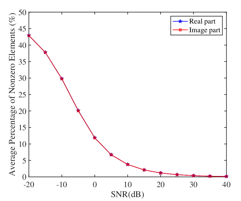
where . To distinguish it from the noise , we call the perturbation vector here. Since the noise is random, it might be possible that only a small portion of the elements of is nonzero. In Figure 1, we plot the average percentage of nonzero elements in with respect to different signal-to-noise ratios (SNRs) when Gaussian noise exists in the signal. It is observed that, when dB, the percentage of nonzero elements in is no more than , i.e., is sparse. Therefore, it is possible to recover the low-rank matrix and the sparse perturbation simultaneously.
To enforce the sparsity of the perturbation vector, we formulate the following one-bit -regularized atomic-norm minimization (1b-ANM- L1) problem:
| (19) |
where is a regularization parameter. This problem is convex and can be directly solved by using the convex optimization toolbox CVX [59].
After solving the problem (19), there are several methods to get the angle and Doppler frequency parameters. One method is to apply the conventional two-dimensional frequency estimation method [52, 53] once the low-rank matrix is recovered. Another method is to explore the two Toeplitz matrices and recovered in (19). By performing Vandermonde decomposition of the two Toeplitz matrices, we can get two sets of frequencies, which correspond to the angles and Doppler frequencies, respectively. Then a simple pairing method, as shown in [57, 58], can be implemented to recover the angle-Doppler pairs. After we get the estimates of the angle-Doppler pairs, the reflection coefficients of the targets can also be estimated. If the number of targets is unknown, we can apply the Bayesian information criterion (BIC) to select the model order. The recently developed one-bit Bayesian information criterion (1bBIC) [39] can be used to determine the model order directly from one-bit measurements. According to Appendix A, we know that . Thus, we can also exploit this property to determine the model order.
V An ADMM-based Iterative Algorithm
Although the convex optimization toolbox can solve the problem (19), it does not scale well when solving large-scale problems. To accelerate the computation, in this section we develop an iterative algorithm to solve the 1b-ANM-L1 problem via the alternating direction method of multipliers (ADMM) [49].
The key to applying the ADMM method is to write out the augmented Lagrangian function of the 1b-ANM-L1 problem. However, due to the last constraint in (19), it is not direct to write out the augmented Lagrangian function. In this section, we introduce a new auxiliary vector , where denotes the element-wise absolute value. Then we can derive the following expression:
| (20) |
where denotes the complex-valued element-wise product of vectors or matrices, i.e., .
First, by applying (20), we rewrite the problem (19) as
| (21) |
where , , and denote the unknown parameters to be optimized, is a regularization parameter, and denotes an indicator function that is 0 if the condition in the bracket is true, and infinity otherwise.
Then the augmented Lagrangian function of the problem (21) can be expressed as
| (22) |
where is the Lagrangian multiplier, and is the penalty parameter.
According to [49], at the -th iteration, the ADMM update takes the following steps:
| (23) |
| (24) |
| (25) |
| (26) |
Since the updates in (24) and (26) is explicit, we derive the updates of (23) and (25) in details. It is noted that the update in (24) is based on the definition of .
V-A Update of , , and
Since it is difficult to solve the problem (23) directly, we update and separately by solving two sub-problems:
| (27) |
| (28) |
For convenience, we introduce the following partitions of the matrices and :
| (29) |
| (30) |
where and are matrices, and are matrices, and and are matrices, respectively.
Then we compute the derivatives of with respect to and the elements of and . The results are given by (31)(33) at the top of this page, where is the -th row of , , and outputs the trace of the -th sub-diagonal of the input matrix.
| (31) |
| (32) |
| (33) |
By setting the derivatives to be 0, , and can be updated by
| (34) |
| (35) |
| (36) |
where denotes the -th column of the matrix .
According to (22), the update of , , is equivalent to solving the following problem:
| (37) |
Therefore, can be updated by
| (38) |
where is the proximal operator [60], in which each element of , denoted as , is given by
| (39) |
Finally, the update of is equivalent to solving the following problem:
| (40) |
The solution is to project the matrix onto the positive definite cone. This projection can be accomplished by setting all the negative eigenvalues of the matrix to zero.
V-B Summary of the ADMM-based Algorithm
The proposed ADMM-based iterative algorithm is summarized as Algorithm 1. It is noted that is initialized to be rather than . If were initialized to be , the term used in (34) would be zero, and the information provided by could not be used in the update process.
VI Performance Analysis based on Cramr-Rao Bound
The Cramr-Rao bound (CRB) provides a theoretical limit on the variance of any unbiased parameter estimator. In this section, we study the effect of one-bit sampling on parameter estimation by analyzing its CRB. Furthermore, based on the derived CRB, two different threshold strategies for one-bit sampling are also discussed.
In our problem, the set of deterministic but unknown parameters to be estimated is , where and denote the magnitude and phase of the reflection coefficient , respectively. We assume that the number of targets, the noise level, and the transmitted signals are known. Since the transmitted signals are known, the operator is deterministic. Each entry of is assumed to be i.i.d. complex Gaussian, i.e., .
VI-A CRB for Unquantized Data
We first establish the CRB for unquantized data. According to (8), the probability density function (PDF) of the unquantized data , denoted as , is expressed as
| (41) |
According to the definition of the Fisher Information Matrix (FIM) of , denoted by , we have
| (42) |
Let and be the real and imaginary parts of , i.e., and . Then (42) can be equivalently expressed as
| (43) |
where
| (44) |
| (45) |
Considering the pulses sent out by the transmitter, the FIM of the set of received unquantized data is
| (46) |
Then the CRB on the variance of the unbiased estimate of the -th parameter is the -th diagonal element of the inverse . Generally, the FIM depends on the values of the parameters.
VI-B CRB for 1-bit Quantized Data
For the one-bit sampled data given in (9), the probability mass function (PMF) of , denoted as , is expressed as
| (47) |
where
| (48) |
and is expressed similarly by replacing with .
Let and be the real and imaginary parts of . Since we have , we can derive that
| (49) |
| (50) |
where . Similar results can be derived for .
By applying the results given in [24], the FIM of the 1-bit quantized data , denoted as , can be stated as
| (51) |
where
| (52) |
| (53) |
with .
With pulses, the FIM becomes
| (54) |
Then the CRB can be determined by the diagonal elements of the inverse .
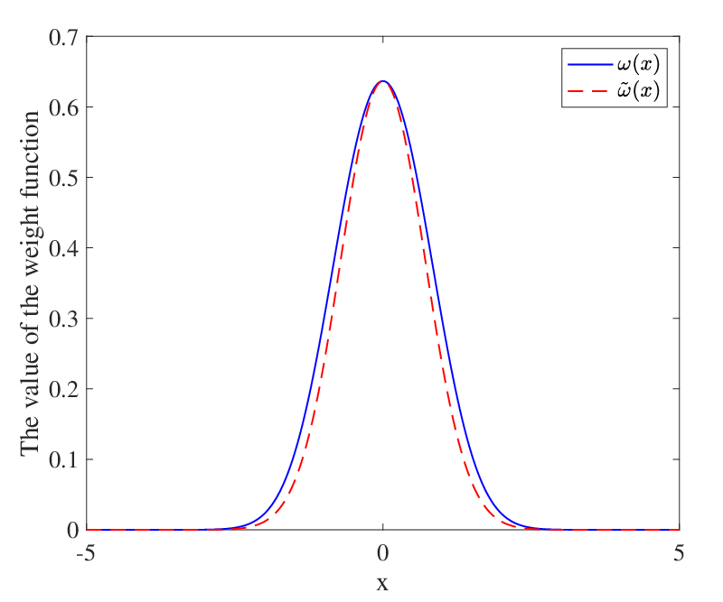
Comparing the results in (52) and (53) with those in (44) and (45), it is seen that the FIM of one-bit sampled data is a weighted version of the FIM of unquantized data, with the weights of for the real part and for the imaginary part. Therefore, the weight function , which is plotted in Fig. 2, has an important effect on the FIM. Considering Fig. 2, we make the following comments on the FIM of one-bit sampled data:
- (i)
The upper bound of is , i.e., . However, in finite SNR scenarios, it is required that and to achieve the upper bound, which is impossible in practical applications. The upper bound also proves that one-bit sampling incurs at least a 2 dB information loss [61].
- (ii)
Given a signal and a threshold, the FIM is closer to its upper bound when the noise variance is larger, i.e., when the SNR is lower. When the SNR increases, the gap between the FIM and its upper bound increases. It is also proved that the parameter estimation performance with one-bit sampling is closer to that with high-bit sampling in the low SNR regime. However, in the high SNR regime, a performance gap separates one-bit sampling and high-bit sampling.
- (iii)
When no threshold is applied, the value of the weight function is inversely proportional to the SNR, i.e., the larger the SNR, the lower the weight function. This relationship leads to significant information loss in the high SNR regime. Thus we prefer to apply the non-zero threshold to one-bit sampling, especially in the high SNR regime. Clearly, designing an appropriate threshold strategy is an important problem in one-bit sampling.
VI-C Threshold Strategies
In this subsection, two different threshold strategies are considered, and the effects of the threshold strategies on the FIM are discussed.
VI-C1 Random Uniform Threshold
The first threshold strategy is to let each element of the threshold and uniformly distributed between and , i.e., .
To simplify our analysis, we approximate the weight function as . The curve of , shown in Fig. 2, approximates the weight function well. Then the expectation of the FIM with respect to the threshold value can be computed as
| (55) |
where , and the last line comes from
| (56) |
with and .
The expectation of the FIM can also be computed similarly. We omit the results here for concision. According to the mean value theorem, there exists a such that
| (57) |
If , is upper bounded by , i.e., . In practice, since we do not know the exact value of , we can set and as the minimum and maximum values of , respectively, such that for every .
VI-C2 Random Gaussian Threshold
The second threshold strategy is to let each element of the threshold be an i.i.d. Gaussian random variable with mean and variance , i.e., . Similarly, .
Then we can derive that
| (58) |
The expectation of the FIM with respect to the threshold value can be approximated as
| (59) |
A similar result can be derived for the FIM . It is noted that the expectation of the weight function depends on only the noise variance and the threshold variance or . If , then (58) becomes , which is independent of the noise variance . This property is useful in improving the performance of one-bit sampling in the high SNR regime. In practice, a priori estimates of and can be set as the mean values of the random Gaussian threshold.
The thresholds we considered here are assumed to be infinite precision, i.e., they can take any value. Actually, due to the finite bit-depth of digital-to-analog converters (DACs), the thresholds have to be quantized to finite precision, i.e., they can take only a set of discrete values.
VI-D CRB for the Case with Unknown Noise Variance
In some practical applications, the noise level in the received signal is unknown. Thus, it is necessary to analyze the CRB under the assumption of unknown noise variance. In this case, the unknown parameters to be estimated become and .
For unquantized data, we can apply the similar analysis in [62] and derive that the FIM can be expressed as
| (60) |
It means that the CRB on the variance of the unbiased estimate of is , and the CRB on the variance of the unbiased estimate of is same as that shown in Section VI-A. The details of the above derivation are omitted here.
For 1-bit quantized data, the FIM becomes
| (61) |
where for with
| (62) |
and
| (63) |
Therefore, the CRBs on the variance of the unbiased estimate of and are the diagonal elements of the inverse of the above Fisher information matrix. The details of the above derivation are given in Appendix B.


VII Numerical Experiments
In this section, we present numerical experiments to illustrate our proposed 1b-MIMO radar, as well as the 1b-ANM-L1 algorithm. As a comparison, two kinds of high-bit quantized MIMO radars are considered. One is a CS-MIMO radar that performs CS in the spatial and Doppler domains but applies 16-bit sampling in the temporal domain. The other is the classic MIMO radar with 16-bit sampling and without any CS techniques.
VII-A Simulation Setup
Throughout the simulations, we consider a MIMO radar with receive antennas and transmit antennas. One CPI includes pulses. A set of quasi-orthogonal waveforms with code length is used as the transmitted waveforms if not specified. For the 1b-MIMO radar and CS-MIMO radar, transmit antennas and receive antennas are randomly chosen. During one CPI, pulses are randomly chosen to send out pulses. With these settings, the total amount of data generated by the 1b-MIMO radar is only as great as the data from the classic MIMO radar, and only of the total data from the CS-MIMO radar. In the 1b-MIMO radar, both the RUT and RGT strategies are implemented to generate the threshold. In the RUT strategy, the threshold is randomly distributed between the minimum value and maximum value of the received signal. In the RGT strategy, the mean of the threshold is the estimates of and provided by the 1b-MIMO radar using RUT 11 1 Here is to show the best achievable performance of the RGT strategy. A more practical way is to use a portion of the data to get a priori estimates., and the variance is . All these thresholds are quantized to 12-bits before applying them to 1-bit sampling. The 1b-MIMO radar and the CS-MIMO radar solve problem (19) and problem (13), respectively. The angle and Doppler frequency are estimated from the recovered low-rank matrix. For the classic MIMO radar, the MEMP method [53] is applied to perform the two-dimensional parameter estimation. To reduce the noise, atomic norm denoising [45] is used after matched filtering. To evaluate the estimation performance, the average mean-squared errors (MSEs) are computed from 200 Monte Carlo runs. In each trial, the noise and threshold are realized independently.
For the proposed ADMM-based 1b-ANM-L1 algorithm, the regularization parameters , , and are set as , , and , respectively. When the normalized error between two iterations is less than or the number of iterations reaches , the ADMM-based iteration is stopped.
VII-B Simulation Results
We first study the estimation accuracy of the 1b-MIMO radar for various SNR values. In this experiment, targets are considered, with normalized spatial frequency (NSF) and normalized Doppler frequency (NDF) pairs of ,,, and . The magnitudes of the reflection coefficients are fixed to be 1, and the phases of the reflection coefficients are randomly distributed between . Note that the last two targets have the same NSFs, i.e., they are located in the same direction. The average MSEs of the NSF and NDF, as well as the probability of successful detection (PSD) with respect to SNR, are shown in Fig. 3(a)(c), respectively. A successful detection is declared if the estimation errors of the NSF and NDF are both less than , i.e., one resolution bin. Only the successful detection trials are taken into account in the computation of the average MSEs. As shown, in the low SNR regime (), the performance of the 1b-MIMO radar is close to the CS-MIMO radar and classic MIMO radar. And in the high SNR regime, the 1b-MIMO radar can achieve MSEs of the NSF and NDF as low as . However, the performance gap between the 1b-MIMO radar and those high-bit quantized rivals increases as the SNR increases. This trend is in accordance with our analysis in Section VI. As shown in Fig. 3(c), the 1b-MIMO radar can achieve a higher PSD in the low SNR regime than its high-bit rivals.


The average MSEs of the magnitude and phase estimation are given in Fig. 3(d)(e), showing that the 1b-MIMO radar with time-varying thresholds can estimate the reflection coefficients of targets with high accuracy. Specially, in the low SNR regime, the 1b-MIMO radar achieves even lower MSEs than its high-bit rivals.
In Fig. 3(f), we plot the normalized low-rank matrix recovery error, defined as , for various SNR values. As SNR increases, the recovery error in the one-bit cases remains close to the CS-MIMO and classic MIMO radars in the low-SNR regime, but it experiences severe performance degeneration in the high-SNR regime. This plot also explains the performance gap between the 1b-MIMO radar and the high-bit quantized rivals in the high SNR regime. Comparing the MSE and CRB curves between the RUT and RGT strategies in Fig. 3(a), (b), (d), and (e), it is clear that, by using the RGT strategy, the performance of the 1b-MIMO radar is significantly better in the high SNR regime. Therefore, designing the optimal threshold to improve performance in the high SNR regime is an important issue for the 1b-MIMO radar.
In Fig. 4, the average CRB of NSF with known noise variance is compared with that with unknown noise variance. It is shown that the two CRB curves are almost the same. The CRBs of other parameters also have the similar results. We omit them here due to length limitation of the paper. We also show the CRB curves approximated by (53) and (57). Although the approximated CRB given by (53) is a little higher than the true CRB of the RUT strategy, (57) approximates the CRB of the RGT strategy quite well.
In Fig. 5, we investigate the estimation performance by using the thresholds with different bit depth. It is shown that, for the RGT strategy, we get lower MSE performance and higher PSD performance in the low SNR regime when using thresholds with higher bit depth. For the RUT strategy, the 1b-MIMO radar using thresholds with different bit depth achieves almost the same MSE and PSD performance.
We next increase the number of samples in the 1b-MIMO radar and demonstrate the MSE performance of the NSF and NDF with respect to . The code length of the corresponding quasi-orthogonal waveforms used in the 1b-MIMO radar also increases as the sampling rate increases. Fig. 6 shows the MSEs of the NSF and NDF estimation, as well as their corresponding CRBs. The MSEs and CRBs of the classic MIMO radar and the CS-MIMO radar with fixed are also shown as benchmarks. As increases, the 1b-MIMO radar improves its estimation performance. Although the total number of bits in the 1b-MIMO radar is still lower than that of its 16-bit rivals, the performance of the 1b-MIMO-RGT radar is close to or even better than that of classic MIMO radar and CS-MIMO radar. These results demonstrate that the performance of the 1b-MIMO radar can be significantly enhanced by increasing the sampling rate. Moreover, it is worth pointing that the cost and energy consumption of a high-rate one-bit ADC may be lower than that of a low-rate high-bit ADC. Therefore, it is possible for 1b-MIMO radar to achieve better performance than its high-bit rivals with lower cost and energy consumption.
Then, to illustrate the performance of the 1b-MIMO radar in resolving multiple closely-located targets, we consider a scenario where there are targets, located with the NSF and NDF pairs , , , . The magnitude of the targets’ reflection coefficients are randomly distributed between , and the phases of the reflection coefficients are randomly distributed between . Thus the targets are separated by one resolution bin in the NSF-NDF plane. We show the average MSEs of the NSF and NDF with respect to different when SNR=40dB in Fig. 7. As the number of targets increases, the MSEs of the NSF and NDF estimation increase from to , which means that the performance of the 1b-MIMO radar deteriorates as the number of targets increases. The gaps between the achieved MSEs and the corresponding CRBs also become larger as increases. However, even when there are targets, the 1b-MIMO radar with both RUT and RGT can still achieve highly accurate NSF and NDF estimations with MSEs as low as . When the number of targets exceeds , the MSEs of the 1b-MIMO radar dramatically increase. In practice, according to our previous definition of successful detection, the 1b-MIMO radar can achieve almost PSD when the number of targets does not exceed .
| Setting I | M=N=T=R=4 | Q=16 | L=64 |
| Setting II | M=N=T=R=6 | Q=36 | L=64 |
| Setting III | M=N=T=R=6 | Q=36 | L=128 |
| Setting IV | M=N=T=R=8 | Q=64 | L=64 |
| Settings | Setting I | Setting II | Setting III | Setting IV |
|---|---|---|---|---|
| ADMM | 6.47s | 24.77s | 37.28s | 99.46s |
| SDPT3 | 40.58s | - | - | - |
| MOSEK | 1.27s | 16.24s | 24.90s | 245.26s |

In Fig. 8, we exploit the distribution of the eigenvalues of recovered in (19) to determine the number of targets . In our method, the estimate of is satisfying , where be the eigenvalues of in descending order. It is shown that the number of targets can be exactly estimated when .
Finally, we compare the running time of the proposed ADMM-based method with the ”brute force” optimization using (19). Two solvers, SDPT3 and MOSEK, in the CVX toolbox [59] are used to solve the ”brute force” optimization. Table II lists the different settings of the 1b-MIMO radar used in this experiment. The other experimental settings are similar to those in Fig. 3. All experiments are carried out in Matlab R2018b on a Mac with a 2.9 GHz Intel Core i9 and 16 GB of RAM. The results are the average value of 200 individual trials. It is seen from Table III that the proposed ADMM algorithm is computationally efficient and scales well as the problem dimension increases. The ”-” in SDPT3 represents that the algorithm is out of memory. The commercial solver MOSEK performs well for Setting I, II, and III. However, the running time of MOSEK increases significantly when the problem dimension becomes large.
VIII Conclusion
This paper discussed the possibility of employing one-bit sampling in MIMO radar to simplify the system’s complexity as well as reduce its hardware cost and energy consumption. To achieve high-resolution angle and Doppler frequency estimation, we developed the 1b-ANM-L1 method to account for the noise perturbations in one-bit sampling. The core idea of the proposed method is that the effect of noise in one-bit sampling can be equivalent to that of sparse impulsive perturbation. To accelerate the computation, an ADMM-based iterative algorithm was derived to compute the solution to the 1b-ANM-L1 problem. The CRB performance of the 1b-MIMO radar with two different threshold strategies was analyzed, which showed that the RGT strategy can improve the performance in high SNR regime by utilizing a priori information. Simulation results showed that, while greatly reducing the amount of data, the 1b-MIMO radar can still achieve high-resolution parameter estimation. The performance of the 1b-MIMO radar could be improved by slightly increasing the sampling rate. Although the 1b-MIMO radar with RGT strategy can achieve performance close to its high-bit rivals, designing the optimal threshold strategy remains an open problem.
Appendix A Proof of Equation (12)
The proof of Equation (12) relies on the classic Vandermonde decomposition of Toeplitz matrices [63, 64], which is summarized in the following lemma.
Lemma A1.
Suppose is a positive semidefinite (PSD) Toeplitz matrix, then admits the following Vandermonde decomposition:
| (A1) |
where is positive definite diagonal matrix, is a Vandermonde matrix whose columns correspond to uniformly sampled complex sinusoids with different frequencies, and . The decomposition is unique if is rank-deficient, i.e., .
Now we give the proof of Equation (12).
Proof:
We first assume that , i.e., admits an order- atomic decomposition , where the pairs of parameters , , are different. Then we can construct the following matrix satisfying the constraint in (12):
| (A2) |
It follows that , where is the optimal solution of the right hand side (RHS) of (12).
On the other hand, when the RHS of (12) achieves the optimal value at the optimizer , there exists a rank- matrix :
| (A3) |
i.e., can be decomposed as:
| (A4) |
where and .
According to Lemma A1, the Toeplitz matrices and admit the following Vandermonde decompositions:
| (A5) |
| (A6) |
where and with , and and are two positive definite diagonal matrices.
Since and , it holds that , , where , and , . Then can be represented as
| (A7) |
This means that each column of lies in the range space spanned by . Similarly, each column of lies in the range space spanned by .
Since has the atomic representation defined in (11), we assume that , where . According to (A7), it holds that and must belong to and , respectively. Therefore, can also be expressed as
| (A8) |
where , and and are matrices with rearranged columns (and maybe replicated columns) of and , respectively. and are two matrices representing the rearrangement and replication operations. Comparing (A7) with (A8), it is equivalent to require that
| (A9) |
If we let and , (A9) is satisfied. In this case, . According to the definition of , we have .
Therefore, we prove that , where is the optimal solution of the RHS of (12).
∎
Appendix B CRB for 1-bit Quantized Data with Unknown Noise Variance
Let be the log-likelihood of the 1-bit quantized data . According to (47), is given as
| (B1) |
where
| (B2) |
and is expressed similarly by replacing and with and , respectively.
Then the derivative of with respective to is given as
| (B3) |
where . Similar result can be derived for . Therefore, we can calculate the following result
| (B4) |
where
| (B5) |
| (B6) |
In the above derivation, we apply the result that .
Furthermore, since , we can derive that
| (B7) |
where
| (B8) |
| (B9) |
Let and , where .
References
- [1] E. Fishler, A. Haimovich, R. Blum, D. Chizhik, L. Cimini, and R. Valenzuela, “MIMO radar: an idea whose time has come,” in Proceedings of the 2004 IEEE Radar Conference, April 2004, pp. 71–78.
- [2] J. Li and P. Stoica, “MIMO radar with colocated antennas,” IEEE Signal Processing Magazine, vol. 24, no. 5, pp. 106–114, Sept 2007.
- [3] A. M. Haimovich, R. S. Blum, and L. J. Cimini, “MIMO radar with widely separated antennas,” IEEE Signal Processing Magazine, vol. 25, no. 1, pp. 116–129, Jan 2008.
- [4] M. Mishali, Y. C. Eldar, O. Dounaevsky, and E. Shoshan, “Xampling: Analog to digital at sub-Nyquist rates,” IET Circuits, Devices Systems, vol. 5, no. 1, pp. 8–20, January 2011.
- [5] S. Becker, “Practical compressed sensing: modern data acquisition and signal processing,” Ph.D. dissertation, California Institute of Technology, 2011.
- [6] F. Xi, S. Chen, and Z. Liu, “Quadrature compressive sampling for radar signals,” IEEE Trans. Signal Process., vol. 62, no. 11, pp. 2787–2802, June 2014.
- [7] O. Bar-Ilan and Y. C. Eldar, “Sub-Nyquist radar via Doppler focusing,” IEEE Trans. Signal Process., vol. 62, no. 7, pp. 1796–1811, April 2014.
- [8] J. Yoo, C. Turnes, E. B. Nakamura, C. K. Le, S. Becker, E. A. Sovero, M. B. Wakin, M. C. Grant, J. Romberg, A. Emami-Neyestanak, and E. Candes, “A compressed sensing parameter extraction platform for radar pulse signal acquisition,” IEEE Journal on Emerging and Selected Topics in Circuits and Systems, vol. 2, no. 3, pp. 626–638, Sep. 2012.
- [9] C. Liu, F. Xi, S. Chen, Y. D. Zhang, and Z. Liu, “Pulse-Doppler signal processing with quadrature compressive sampling,” IEEE Trans. Aerosp. Electron. Syst., vol. 51, no. 2, pp. 1217–1230, April 2015.
- [10] Y. Yu, A. P. Petropulu, and H. V. Poor, “MIMO radar using compressive sampling,” IEEE Journal of Selected Topics in Signal Processing, vol. 4, no. 1, pp. 146–163, Feb 2010.
- [11] S. Sun, W. U. Bajwa, and A. P. Petropulu, “MIMO-MC radar: A mimo radar approach based on matrix completion,” IEEE Transactions on Aerospace and Electronic Systems, vol. 51, no. 3, pp. 1839–1852, July 2015.
- [12] M. Rossi, A. M. Haimovich, and Y. C. Eldar, “Spatial compressive sensing for MIMO radar,” IEEE Transactions on Signal Processing, vol. 62, no. 2, pp. 419–430, Jan 2014.
- [13] D. Cohen, D. Cohen, Y. C. Eldar, and A. M. Haimovich, “SUMMeR: Sub-Nyquist MIMO Radar,” IEEE Transactions on Signal Processing, vol. 66, no. 16, pp. 4315–4330, 2018.
- [14] D. Cohen and Y. C. Eldar, “Reduced time-on-target in pulse doppler radar: Slow time domain compressed sensing,” in 2016 IEEE Radar Conference (RadarConf), May 2016, pp. 1–4.
- [15] S. Na, K. V. Mishra, Y. Liu, Y. C. Eldar, and X. Wang, “TenDSuR: Tensor-based 4D sub-Nyquist radar,” IEEE Signal Processing Letters, vol. 26, no. 2, pp. 237–241, Feb 2019.
- [16] D. Cohen and Y. C. Eldar, “Sub-Nyquist radar systems: Temporal, spectral, and spatial compression,” IEEE Signal Processing Magazine, vol. 35, no. 6, pp. 35–58, Nov 2018.
- [17] R. H. Walden, “Analog-to-digital converter survey and analysis,” IEEE Journal on Selected Areas in Communications, vol. 17, no. 4, pp. 539–550, April 1999.
- [18] T. W. Rondeau, J. H. Reed, and C. W. Bostian, “Analog-to-digital converters,” IEEE Signal Processing Magazine, vol. 22, no. 6, pp. 69–77, Nov 2005.
- [19] P. T. Boufounos and R. G. Baraniuk, “1-bit compressive sensing,” in 2008 42nd Annual Conference on Information Sciences and Systems, March 2008, pp. 16–21.
- [20] J. N. Laska, Z. Wen, W. Yin, and R. G. Baraniuk, “Trust, but verify: Fast and accurate signal recovery from 1-bit compressive measurements,” IEEE Transactions on Signal Processing, vol. 59, no. 11, pp. 5289–5301, Nov 2011.
- [21] L. Jacques, J. N. Laska, P. T. Boufounos, and R. G. Baraniuk, “Robust 1-bit compressive sensing via binary stable embeddings of sparse vectors,” IEEE Transactions on Information Theory, vol. 59, no. 4, pp. 2082–2102, April 2013.
- [22] C. Gianelli, L. Xu, J. Li, and P. Stoica, “One-bit compressive sampling with time-varying thresholds for multiple sinusoids,” in 2017 IEEE 7th International Workshop on Computational Advances in Multi-Sensor Adaptive Processing (CAMSAP), Dec 2017, pp. 1–5.
- [23] C. Qian and J. Li, “ADMM for harmonic retrieval from one-bit sampling with time-varying thresholds,” in 2017 IEEE International Conference on Acoustics, Speech and Signal Processing (ICASSP), March 2017, pp. 3699–3703.
- [24] H. Fu and Y. Chi, “Quantized spectral compressed sensing: Cramer–Rao bounds and recovery algorithms,” IEEE Transactions on Signal Processing, vol. 66, no. 12, pp. 3268–3279, June 2018.
- [25] O. Bar-Shalom and A. J. Weiss, “DOA estimation using one-bit quantized measurements,” IEEE Transactions on Aerospace and Electronic Systems, vol. 38, no. 3, pp. 868–884, July 2002.
- [26] K. Yu, Y. D. Zhang, M. Bao, Y. H. Hu, and Z. Wang, “DOA estimation from one-bit compressed array data via joint sparse representation,” IEEE Signal Processing Letters, vol. 23, no. 9, pp. 1279–1283, Sept 2016.
- [27] J. Li, M. M. Naghsh, S. J. Zahabi, and M. Modarres-Hashemi, “Compressive radar sensing via one-bit sampling with time-varying thresholds,” in 2016 50th Asilomar Conference on Signals, Systems and Computers, Nov 2016, pp. 1164–1168.
- [28] S. J. Zahabi, M. M. Naghsh, M. Modarres-Hashemi, and J. Li, “Compressive pulse-Doppler radar sensing via 1-bit sampling with time-varying threshold,” in 2017 IEEE International Conference on Acoustics, Speech and Signal Processing (ICASSP), March 2017, pp. 3419–3423.
- [29] F. Xi and S. Chen, “Super-resolution pulse-Doppler radar sensing via one-bit sampling,” in 2018 IEEE 10th Sensor Array and Multichannel Signal Processing Workshop (SAM), July 2018, pp. 232–236.
- [30] Y. Li, C. Tao, G. Seco-Granados, A. Mezghani, A. L. Swindlehurst, and L. Liu, “Channel estimation and performance analysis of one-bit massive MIMO systems,” IEEE Transactions on Signal Processing, vol. 65, no. 15, pp. 4075–4089, Aug 2017.
- [31] M. S. Stein, S. Bar, J. A. Nossek, and J. Tabrikian, “Performance analysis for channel estimation with 1-bit ADC and unknown quantization threshold,” IEEE Transactions on Signal Processing, vol. 66, no. 10, pp. 2557–2571, May 2018.
- [32] F. Wang, J. Fang, H. Li, Z. Chen, and S. Li, “One-bit quantization design and channel estimation for massive MIMO systems,” IEEE Transactions on Vehicular Technology, vol. 67, no. 11, pp. 10 921–10 934, Nov 2018.
- [33] K. Knudson, R. Saab, and R. Ward, “One-bit compressive sensing with norm estimation,” IEEE Transactions on Information Theory, vol. 62, no. 5, pp. 2748–2758, May 2016.
- [34] V. Cambareri and L. Jacques, “Time for dithering: fast and quantized random embeddings via the restricted isometry property,” Information and Inference: A Journal of the IMA, vol. 6, no. 4, pp. 441–476, 04 2017.
- [35] L. Jacques, “Small width, low distortions: Quantized random embeddings of low-complexity sets,” IEEE Transactions on Information Theory, vol. 63, no. 9, pp. 5477–5495, Sep. 2017.
- [36] C. Xu and L. Jacques, “Quantized compressive sensing with RIP matrices: The benefit of dithering,” CoRR, vol. abs/1801.05870, 2018.
- [37] S. Khobahi and M. Soltanalian, “Signal recovery from 1-bit quantized noisy samples via adaptive thresholding,” in 2018 52nd Asilomar Conference on Signals, Systems, and Computers, Oct 2018, pp. 1757–1761.
- [38] Y. Plan and R. Vershynin, “Robust 1-bit compressed sensing and sparse logistic regression: A convex programming approach,” IEEE Transactions on Information Theory, vol. 59, no. 1, pp. 482–494, Jan 2013.
- [39] P. T. Boufounos, “Greedy sparse signal reconstruction from sign measurements,” in 2009 Conference Record of the Forty-Third Asilomar Conference on Signals, Systems and Computers, Nov 2009, pp. 1305–1309.
- [40] M. Yan, Y. Yang, and S. Osher, “Robust 1-bit compressive sensing using adaptive outlier pursuit,” IEEE Transactions on Signal Processing, vol. 60, no. 7, pp. 3868–3875, July 2012.
- [41] Y. Chi, L. L. Scharf, A. Pezeshki, and A. R. Calderbank, “Sensitivity to basis mismatch in compressed sensing,” IEEE Trans. Signal Process., vol. 59, no. 5, pp. 2182–2195, May 2011.
- [42] J. Ren, T. Zhang, J. Li, and P. Stoica, “Sinusoidal parameter estimation from signed measurements via majorization–minimization based relax,” IEEE Transactions on Signal Processing, vol. 67, no. 8, pp. 2173–2186, April 2019.
- [43] E. J. Candes and C. Fernandez-Granda, “Towards a mathematical theory of super-resolution,” Communications on Pure and Applied Mathematics, vol. 67, no. 6, pp. 906–956, 2014.
- [44] G. Tang, B. N. Bhaskar, P. Shah, and B. Recht, “Compressed sensing off the grid,” IEEE Trans. Inf. Theory, vol. 59, no. 11, pp. 7465–7490, Nov 2013.
- [45] B. N. Bhaskar, G. Tang, and B. Recht, “Atomic norm denoising with applications to line spectral estimation,” IEEE Transactions on Signal Processing, vol. 61, no. 23, pp. 5987–5999, Dec 2013.
- [46] Z. Yang and L. Xie, “On gridless sparse methods for line spectral estimation from complete and incomplete data,” IEEE Trans. Signal Process., vol. 63, no. 12, pp. 3139–3153, June 2015.
- [47] Z. Yang, L. Xie, and P. Stoica, “Vandermonde decomposition of multilevel toeplitz matrices with application to multidimensional super-resolution,” IEEE Transactions on Information Theory, vol. 62, no. 6, pp. 3685–3701, June 2016.
- [48] Z. Zhang, Y. Wang, and Z. Tian, “Efficient two-dimensional line spectrum estimation based on decoupled atomic norm minimization,” Signal Processing, vol. 163, pp. 95 – 106, 2019.
- [49] S. Boyd, N. Parikh, E. Chu, B. Peleato, and J. Eckstein, “Distributed optimization and statistical learning via the alternating direction method of multipliers,” Found. Trends Mach. Learn., vol. 3, no. 1, pp. 1–122, Jan. 2011.
- [50] L. Zheng and X. Wang, “Super-resolution delay-doppler estimation for ofdm passive radar,” IEEE Transactions on Signal Processing, vol. 65, no. 9, pp. 2197–2210, May 2017.
- [51] M. Richards, Fundamentals of Radar Signal Processing. New York, NY, USA: McGraw-Hill, 2005.
- [52] S. Kay and R. Nekovei, “An efficient two-dimensional frequency estimator,” IEEE Transactions on Acoustics, Speech, and Signal Processing, vol. 38, no. 10, pp. 1807–1809, Oct 1990.
- [53] Y. Hua, “Estimating two-dimensional frequencies by matrix enhancement and matrix pencil,” IEEE Transactions on Signal Processing, vol. 40, no. 9, pp. 2267–2280, Sep. 1992.
- [54] X. Wang, E. Aboutanios, M. Trinkle, and M. G. Amin, “Reconfigurable adaptive array beamforming by antenna selection,” IEEE Transactions on Signal Processing, vol. 62, no. 9, pp. 2385–2396, May 2014.
- [55] B. Li and A. P. Petropulu, “Joint transmit designs for coexistence of MIMO wireless communications and sparse sensing radars in clutter,” IEEE Transactions on Aerospace and Electronic Systems, vol. 53, no. 6, pp. 2846–2864, Dec 2017.
- [56] J. Qian, M. Lops, , X. Wang, and Z. He, “Joint system design for coexistence of MIMO radar and MIMO communication,” IEEE Transactions on Signal Processing, vol. 66, no. 13, pp. 3504–3519, July 2018.
- [57] F. Xi, S. Chen, and Z. Liu, “Super-resolution delay-Doppler estimation for sub-Nyquist radar via atomic norm minimization,” in 2017 IEEE International Conference on Acoustics, Speech and Signal Processing (ICASSP), March 2017, pp. 4326–4330.
- [58] Z. Tian, Z. Zhang, and Y. Wang, “Low-complexity optimization for two-dimensional direction-of-arrival estimation via decoupled atomic norm minimization,” in 2017 IEEE International Conference on Acoustics, Speech and Signal Processing (ICASSP), March 2017, pp. 3071–3075.
- [59] M. Grant and S. Boyd, “CVX: Matlab software for disciplined convex programming, version 2.1,” http://cvxr.com/cvx, Mar. 2014.
- [60] A. Maleki, L. Anitori, Z. Yang, and R. G. Baraniuk, “Asymptotic analysis of complex LASSO via complex approximate message passing (CAMP),” IEEE Transactions on Information Theory, vol. 59, no. 7, pp. 4290–4308, July 2013.
- [61] H. C. Papadopoulos, G. W. Wornell, and A. V. Oppenheim, “Sequential signal encoding from noisy measurements using quantizers with dynamic bias control,” IEEE Transactions on Information Theory, vol. 47, no. 3, pp. 978–1002, March 2001.
- [62] P. Stoica and A. Nehorai, “Music, maximum likelihood, and cramer-rao bound,” IEEE Transactions on Acoustics, Speech, and Signal Processing, vol. 37, no. 5, pp. 720–741, May 1989.
- [63] C. Carathéodory and L. Fejér, “Über den zusammenhang der extremen von harmonischen funktionen mit ihren koeffizienten und über den picard-landau’schen satz,” Rendiconti del Circolo Matematico di Palermo (1884-1940), vol. 32, no. 1, pp. 218–239, 1911.
- [64] P. Stoica and R. L. Moses, Spectral analysis of signals. NJ, USA: Pearson/Prentice Hall Upper Saddle River, 2005.