跳到论文正文
W Papers独立论文阅读器 arXiv:1908.10434 论文正文 计算阅读时间 · 0%
引用这篇论文根据当前论文元数据生成,正式投稿前建议核对。


License: arXiv.org perpetual non-exclusive license
arXiv:1908.10434v2 [math.DG] 27 Oct 2020

Special elliptic isometries, relative SU(2,1)\mathop{\mathrm{SU}}(2,1)-character varieties, and bendings

Felipe A. Franco Note: Supported by grant 2014/00582-2, São Paulo Research Foundation (FAPESP), and by CNPq.    Carlos H. Grossi
Abstract

We study relations between special elliptic isometries in the complex hyperbolic plane. Relations of lengths 22, 33, and 44 are fully classified. Some relative SU(2,1)\mathop{\mathrm{SU}}(2,1)-character varieties of the quadruply punctured sphere are described and applied to the study of length 55 relations.

1 Introduction

Relations between automorphisms of a given geometric structure play an important role in the construction of manifolds/orbifolds endowed with that geometric structure. Consider, for instance, Poincaré’s Polyhedron Theorem, which is one of the few known tools for the construction of manifolds/orbifolds equipped with some model geometry (typically, a simply-connected Riemannian manifold). Roughly speaking, the theorem specifies conditions on a polyhedron with side-pairing isometries in the model space XX such that the group HH generated by these isometries is discrete and X/HX/H is a manifold/orbifold MM modelled on XX. The group HH is isomorphic to the fundamental group π1​(M)\pi_{1}(M) and the theorem provides an explicit presentation of HH that comes from the combinatorial structure of the polyhedron with face-pairing isometries. This means that, in a certain sense, in order to construct a polyhedron with side-pairing isometries that have a chance of succeeding as a fundamental polyhedron, some relations between those isometries of XX that will play the role of side-pairing isometries must be known a priori.11 1 For example, the study of short relations between isometries in the complex hyperbolic plane plays an important role in the construction of complex hyperbolic disc bundles in [5] and in [6].

More generally, the space of representations of the fundamental group π1​(M)\pi_{1}(M) in some group GG of automorphisms of the model space modulo conjugation, i.e., the GG-character variety of MM, is closely related to the geometric structures on MM inherited from the model space. Hence, it is natural to expect that (relative) character varieties are ubiquitous objects in geometry and that the many questions related to its structure (topology, Hitchin components, nature of the action of the mapping class group, etc.) are sources of great interest. They have been investigated by several authors, and an exhaustive list of references would be too long to compile; so, we only cite a few ones [1], [7], [9], [12], [14], [15], [19] which are closer to this paper.

Here, our model space is the complex hyperbolic plane ℍℂ2\mathbb{H}^{2}_{\mathbb{C}} with orientation-preserving isometries or, equivalently, the holomorphic 22-ball with its complex automorphisms; the corresponding group is the projective unitary group PU(2,1)\mathop{\mathrm{PU}}(2,1). A rough classification of nontrivial orientation-preserving isometries in the complex hyperbolic plane resembles that of constant curvature hyperbolic geometry: they either have a fixed point in ℍℂ2\mathbb{H}^{2}_{\mathbb{C}} (elliptic isometries), exactly one fixed point in the ideal boundary of ℍℂ2\mathbb{H}^{2}_{\mathbb{C}} (parabolic isometries), or exactly two fixed points in this ideal boundary (loxodromic isometries). Each of these isometry types are divided into several subtypes whose geometric behaviour can be quite different from each other (see Subsection 2.1). Of central interest in this paper is the subtype of elliptic isometries known as the special ones. This subtype includes the holomorphic involutions.

Holomorphic involutions generate the group of orientation-preserving isometries of ℍℂ2\mathbb{H}^{2}_{\mathbb{C}}. They come in two conjugacy classes: reflections in (negative) points and reflections in complex geodesics (or in positive points). The decomposition of orientation-preserving isometries into the product of involutions is considered in [2] and in [19]. An interesting question is to understand to what extent such a decomposition is unique. This naturally leads to the study of relative character varieties that encode all the possible decompositions, modulo conjugation, of a given isometry into the product of involutions [2, Section 4] and to the concept of bendings. In a nutshell, bendings provide natural coordinates in the mentioned relative character varieties. More precisely, let RpR^{p} stand for the reflection in a negative or positive point pp and consider a relation Rpn​…​Rp2​Rp1=1R^{p_{n}}\ldots R^{p_{2}}R^{p_{1}}=1 between holomorphic involutions in PU(2,1)\mathop{\mathrm{PU}}(2,1). If we move the points pi−1,pip_{i-1},p_{i} along a geodesic that joins them without altering their distance, we obtain new points qi−1,qiq_{i-1},q_{i} satisfying Rqi​Rqi−1=Rpi​Rpi−1R^{q_{i}}R^{q_{i-1}}=R^{p_{i}}R^{p_{i-1}}. This alters the original relation Rpn​…​Rpi​Rpi−1​…​Rp2​Rp1=1R^{p_{n}}\ldots R^{p_{i}}R^{p_{i-1}}\ldots R^{p_{2}}R^{p_{1}}=1 into the new one Rpn​…​Rqi​Rqi−1​…​Rp1=1R^{p_{n}}\ldots R^{q_{i}}R^{q_{i-1}}\ldots R^{p_{1}}=1 and is the same as taking an element CC in the centralizer of Rpi​Rpi−1R^{p_{i}}R^{p_{i-1}} and writing Rpi​Rpi−1=(C​Rpi​C−1)​(C​Rpi−1​C−1)=RC​pi​RC​pi−1=Rqi​Rqi−1R^{p_{i}}R^{p_{i-1}}=(CR^{p_{i}}C^{-1})(CR^{p_{i-1}}C^{-1})=R^{Cp_{i}}R^{Cp_{i-1}}=R^{q_{i}}R^{q_{i-1}}.

Sometimes, a relation between holomorphic involutions of the above form can be simplified by bending it and applying afterwards the length 22 relation Rp​Rp=1R^{p}R^{p}=1 (a cancellation which can appear when neighbouring involutions in the relation become equal after a bending) or a length 33 relation known as an orthogonal relation [2]. It is worthwhile mentioning that length 55 relations between holomorphic involutions that cannot be simplified in such a way, that is, basic length 55 relations, have been linked to discreteness [2], [3].

In this paper, we consider relations between special elliptic isometries. Special elliptic isometries can be seen as rotations around (negative) points or rotations around complex geodesics (equivalently, around positive points). Since every orientation-preserving isometry has three lifts to SU(2,1)\mathop{\mathrm{SU}}(2,1) that differ by a cube root of unity, a nontrivial special elliptic isometry is determined, at the level of SU(2,1)\mathop{\mathrm{SU}}(2,1), by a (negative or positive) point pp, its centre, and by a unit complex number α\alpha distinct from a cube root of unity, its parameter. Throughout the paper, we deal with elements in SU(2,1)\mathop{\mathrm{SU}}(2,1); so, we write a relation between special elliptic isometries in the form Rαnpn​…​Rα2p2​Rα1p1=δR_{\alpha_{n}}^{p_{n}}\ldots R_{\alpha_{2}}^{p_{2}}R_{\alpha_{1}}^{p_{1}}=\delta, where δ\delta is a cube root of unity, and refer to Rαnpn​…​Rα2p2​Rα1p1=δR_{\alpha_{n}}^{p_{n}}\ldots R_{\alpha_{2}}^{p_{2}}R_{\alpha_{1}}^{p_{1}}=\delta as a length nn relation.

Relations between special elliptic isometries of lengths 22 and 33, as well as the length 44 ones obtained through bendings, are quite similar to those between holomorphic involutions and are described in Sections 3 and 4. On the other hand, the full description of length 44 relations in Theorem 6.23, one of the main results of the paper, is much more involved and requires a new set of tools which are particularly technical. For that reason, it is postponed until Section 6.

Equipped with bendings, we are able to consider the decompositions of regular orientation-preserving isometries (see Definition 2.2) in the product of three special elliptic ones. (This is in fact the main part of the study of length 55 relations between special elliptic isometries since such relations can be written in the form Rα3p3​Rα2p2​Rα1p1=Rβ2q2​Rβ1q1R_{\alpha_{3}}^{p_{3}}R_{\alpha_{2}}^{p_{2}}R_{\alpha_{1}}^{p_{1}}=R_{\beta_{2}}^{q_{2}}R_{\beta_{1}}^{q_{1}} and Rβ2q2​Rβ1q1R_{\beta_{2}}^{q_{2}}R_{\beta_{1}}^{q_{1}} is a regular orientation-preserving isometry.) These decompositions naturally lead to the description, given in Theorem 5.9 (see also Theorem 5.2) of some relative SU(2,1)\mathop{\mathrm{SU}}(2,1)-character varieties consisting of representations ρ:π1​(Σ)→SU(2,1)\rho:\pi_{1}(\Sigma)\to\mathop{\mathrm{SU}}(2,1), modulo conjugation, of the rank 33 free group π1(Σ):=⟨ι1,ι2,ι3,ι4∣ι4ι3ι2ι1=1⟩\pi_{1}(\Sigma):=\langle\iota_{1},\iota_{2},\iota_{3},\iota_{4}\mid\iota_{4}\iota_{3}\iota_{2}\iota_{1}=1\rangle (the fundamental group of the quadruply punctured sphere Σ\Sigma), where the conjugacy classes of ρ⁡(ιi)\rho(\iota_{i}) are those of special elliptic isometries, i=1,2,3i=1,2,3, and the conjugacy class of ρ⁡(ι4)\rho(\iota_{4}) is that of a regular isometry in SU(2,1)\mathop{\mathrm{SU}}(2,1). These relative character varieties are (as is typical) semialgebraic surfaces SS whose nature, studied in Theorem 5.4, allows us to obtain a simple condition guaranteeing that a couple of given points in SS lie in a same connected component and, in particular, can be connected, modulo conjugation, by finitely many bendings (Corollary 5.11). Incidently, an unexpected consequence of Theorem 5.4 is a criterion determining the type of an isometry of the form Rα2p2​Rα1p1R_{\alpha_{2}}^{p_{2}}R_{\alpha_{1}}^{p_{1}} in terms of centres and parameters.

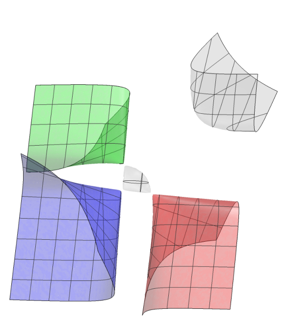
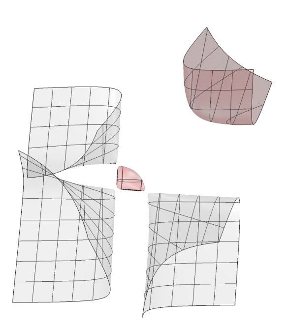
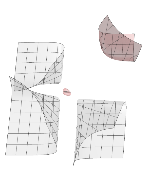
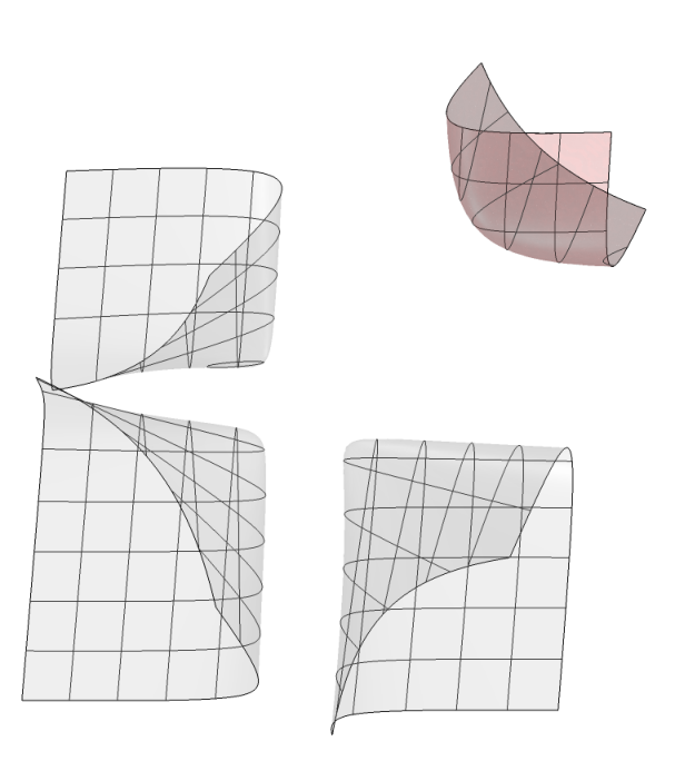
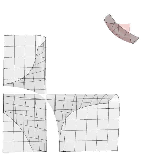
Some experimental observations regarding the semialgebraic surface SS, as well as many pictures illustrating its behaviour, can be seen on Subsection 5.12.

It is worthwhile mentioning that the study of the possible conjugacy classes of the product of a pair of isometries have been considered in [11], [18], and [19]. It is formulated in terms of the product map 𝒞1×𝒞2→𝒢\mathcal{C}_{1}\times\mathcal{C}_{2}\to\mathcal{G}, (A,B)↦[A​B](A,B)\mapsto[AB], where 𝒢\mathcal{G} denotes the space of all PU(2,1)\mathop{\mathrm{PU}}(2,1)-conjugacy classes, 𝒞1,𝒞2∈𝒢\mathcal{C}_{1},\mathcal{C}_{2}\in\mathcal{G}, and [A​B][AB] stands for the PU(2,1)\mathop{\mathrm{PU}}(2,1)-conjugacy class of the product A​BAB. In our context, the vertical and horizontal slices in Theorem 5.4 can be seen as fibres of the product map. Moreover, the image by the product map of a degenerate slice (see Definition 5.6) is a point in a reducible wall (see [18] for the definition of reducible wall).

Finally, in Section 6, we complete the classification of length 44 relations between special elliptic isometries. The ff-bendings play a major role in this classification. Similarly to bendings, they can also be seen as one-parameter deformations of a given product Rα2p2​Rα1p1R_{\alpha_{2}}^{p_{2}}R_{\alpha_{1}}^{p_{1}} of special elliptic isometries; such deformation is geometrically described in Theorem 6.5. However, during an ff-bending, both the centres and the parameters change. An ff-bending preserves the signs of the centres as well as the components (see Definition 4.4) and the product of the parameters. Every (generic) length 44 relation of the form Rα2p2​Rα1p1=Rβ2q2​Rβ1q1R_{\alpha_{2}}^{p_{2}}R_{\alpha_{1}}^{p_{1}}=R_{\beta_{2}}^{q_{2}}R_{\beta_{1}}^{q_{1}}, where pi,qip_{i},q_{i} are points of a same sign and αi,βi\alpha_{i},\beta_{i} are parameters in a same component, is a consequence of bendings and ff-bendings (Theorem 6.11). Dropping these restrictions on signs and components, we found it necessary to develop some new tools in order to complete the classification of (generic) length 44 isometries (in total, there are 77 “basic” relations of length 44). These tools regard the behaviour of some naturally parameterized lines tangent to Goldman’s deltoid (Proposition 6.20) as well as a characterization allowing to determine when regular elliptic isometries of the same trace written as products of two special elliptic isometries belong to the same SU(2,1)\mathop{\mathrm{SU}}(2,1)-conjugacy class (Proposition 6.15).

As applications of the techniques developed in Sections 5 and 6, we show that special elliptic pentagons, i.e., some length 55 relations between special elliptic isometries, can be connected modulo conjugation by finitely many bendings (see Theorem 7.3) as well as by finitely many bendings and ff-bendings (see Theorem 7.5), as long as the appropriate natural conditions are required in each case.

Acknowledgments. We are very grateful to the anonymous referee whose careful suggestions have greatly improved the paper.

2 Complex hyperbolic geometry

In this section we briefly discuss some basic aspects of plane complex hyperbolic geometry. Our approach essentially follows [4], [5], and [13].

Let VV be a 3-dimensional ℂ\mathbb{C}-linear space equipped with a Hermitian form ⟨−,−⟩\left<-,-\right> of signature ++−++-. We frequently use the same letter to denote both a point in the complex projective plane ℙ​V\mathbb{P}V and a representative in VV.

The complex projective plane ℙ​V\mathbb{P}V is divided into negative, isotropic, and positive points:

B​V:={p∈ℙ​V|⟨p,p⟩<0},S​V:={p∈ℙ​V|⟨p,p⟩=0},E​V:={p∈ℙ​V|⟨p,p⟩>0}.{\mathrm{B}}\,V:=\left\{p\in{\mathbb{P}}V\,|\,\left<p,p\right><0\right\},\ \ {\mathrm{S}}\,V:=\left\{p\in{\mathbb{P}}V\,|\,\left<p,p\right>=0\right\},\ {\mathrm{E}}\,V:=\{p\in\mathbb{P}V\,|\,\left<p,p\right>>0\}.

The signature σ​p\sigma p of a point p∈ℙ​Vp\in\mathbb{P}V is respectively −1,0,1-1,0,1 when pp is negative, isotropic, positive. It is easy to see that B​V{\mathrm{B}}\,V is a (real) 44-dimensional open ball whose boundary S​V{\mathrm{S}}\,V is a 33-sphere.

Let p∈ℙ​V∖S​Vp\in\mathbb{P}V\setminus{\mathrm{S}}\,V be a nonisotropic point. There is a well-known natural identification

Tp​ℙ​V≃Linℂ​(ℂ​p,p⊥)=⟨−,p⟩​p⊥\mathrm{T}_{p}\mathbb{P}V\simeq{\mathrm{Lin}}_{\mathbb{C}}(\mathbb{C}p,p^{\bot})=\left<-,p\right>p^{\bot} (1)

where p⟂p^{\perp} stands for the linear subspace orthogonal to pp and ⟨−,p⟩\langle-,p\rangle denotes the linear functional x↦⟨x,p⟩x\mapsto\langle x,p\rangle.

Both B​V{\mathrm{B}}\,V and E​V{\mathrm{E}}\,V are endowed with the Hermitian metric defined by

⟨t1,t2⟩:=−⟨t1​(p),t2​(p)⟩⟨p,p⟩\langle t_{1},t_{2}\rangle:=-\frac{\big\langle t_{1}(p),t_{2}(p)\big\rangle}{\langle p,p\rangle}

where t1,t2∈Lin⁡(ℂ​p,p⟂)t_{1},t_{2}\in\mathrm{Lin}(\mathbb{C}p,p^{\perp}) are tangent vectors at the nonisotropic point pp. This Hermitian metric is positive-definite on B​V{\mathrm{B}}\,V and of signature +⁣−+- on E​V{\mathrm{E}}\,V. In particular, we obtain a Riemannian metric on B​V{\mathrm{B}}\,V. Equipped with such metric, B​V{\mathrm{B}}\,V is called the complex hyperbolic plane and is denoted by ℍℂ2\mathbb{H}_{\mathbb{C}}^{2}. Its ideal boundary, also known as the absolute, is the 33-sphere S​V{\mathrm{S}}\,V of isotropic points. Note that E​V{\mathrm{E}}\,V is a pseudo-Riemannian manifold; a simple duality, discussed below, shows that it is the space of complex lines intersecting B​V{\mathrm{B}}\,V.

Let L⊂ℙ​VL\subset\mathbb{P}V be a complex line, i.e., the projectivization ℙ​W\mathbb{P}W of a complex 22-dimensional subspace W⩽VW\leqslant V. The point c:=ℙ​W⟂c:=\mathbb{P}W^{\perp} is called the polar of LL. By Sylvester’s criterion, the signature of the Hermitian form restricted to WW can be +⁣−+-, +⁣+++, or +0+0. The corresponding complex line is respectively called hyperbolic, spherical, or Euclidean. Clearly, a projective line is hyperbolic, spherical, or Euclidean exactly when its polar point is positive, negative, or isotropic. The negative part L∩B​VL\cap{\mathrm{B}}\,V of a hyperbolic complex line LL is often called a complex geodesic. Given two distinct points p1,p2∈ℙ​Vp_{1},p_{2}\in\mathbb{P}V, the (unique) complex line ℙ⁡(ℂ​p1+ℂ​p2)\mathbb{P}(\mathbb{C}p_{1}+\mathbb{C}p_{2}) containing p1,p2p_{1},p_{2} is denoted L⁡(p1,p2)\mathrm{L}(p_{1},p_{2}). The following simple facts concerning complex lines will be regularly used throughout the paper:

The restriction L∩B​VL\cap{\mathrm{B}}\,V of a hyperbolic line to B​V{\mathrm{B}}\,V is a totally geodesic subspace of constant curvature (a Poincaré disc). The same holds for L∩E​VL\cap{\mathrm{E}}\,V. The geometry of a spherical complex line is that of a round sphere.

Arbitrary complex lines L1,L2L_{1},L_{2} are either equal or have a single common point in ℙ​V\mathbb{P}V. A pair of complex lines L1,L2L_{1},L_{2} is said to be orthogonal iff the polar point of L1L_{1} belongs to L2L_{2} (or, equivalently, the polar point of L2L_{2} belongs to L1L_{1}). When the lines are noneuclidean, this means that they are orthogonal in the sense of the Hermitian metric. Given a point pp in a complex line LL, there exists a unique point p~∈L\tilde{p}\in L such that ⟨p,p~⟩=0\langle p,\tilde{p}\rangle=0 (in the Euclidean case, p=p~p=\tilde{p}).

A useful criterion to decide the type of the complex line L:=L⁡(p1,p2)L:=\mathrm{L}(p_{1},p_{2}) in terms of nonisotropic, nonorthogonal, distinct spanning points p1,p2p_{1},p_{2} involves the tance

ta(p1,p2):=⟨p1,p2⟩​⟨p2,p1⟩⟨p1,p1⟩​⟨p2,p2⟩.\mathop{\mathrm{ta}}(p_{1},p_{2}):=\frac{\left<p_{1},p_{2}\right>\left<p_{2},p_{1}\right>}{\left<p_{1},p_{1}\right>\left<p_{2},p_{2}\right>}.

By Sylvester’s criterion, the line LL is hyperbolic when ta(p1,p2)>1\mathop{\mathrm{ta}}(p_{1},p_{2})>1 or ta(p1,p2)<0\mathop{\mathrm{ta}}(p_{1},p_{2})<0; Euclidean when ta(p1,p2)=1\mathop{\mathrm{ta}}(p_{1},p_{2})=1; spherical when 0<ta(p1,p2)<10<\mathop{\mathrm{ta}}(p_{1},p_{2})<1. Note that, for p1,p2∈B​Vp_{1},p_{2}\in{\mathrm{B}}\,V, we have ta(p1,p2)⩾1\mathop{\mathrm{ta}}(p_{1},p_{2})\geqslant 1 and ta(p1,p2)=1\mathop{\mathrm{ta}}(p_{1},p_{2})=1 iff p1=p2p_{1}=p_{2}.

An extended geodesic in ℙ​V\mathbb{P}V is, by definition, the (complex) projectivization ℙ​W\mathbb{P}W of an ℝ\mathbb{R}-linear subspace WW of VV, dimℝW=2\dim_{\mathbb{R}}W=2, such that the Hermitian form, being restricted to WW, is real and does not vanish (ℙ​W\mathbb{P}W stands for π⁡(W∖{0})\pi(W\setminus\{0\}), where π:V∖{0}→ℙ​V\pi:V\setminus\{0\}\to\mathbb{P}V is the canonical projection). Every extended geodesic is a topological circle contained in a unique complex line. The usual Riemannian geodesics in ℍℂ2\mathbb{H}_{\mathbb{C}}^{2} are the restrictions ℙ​W∩B​V\mathbb{P}W\cap{\mathrm{B}}\,V [4, Corollary 5.5] (the same holds for the usual pseudo-Riemannian geodesics in E​V{\mathrm{E}}\,V).

The following simple facts concerning extended geodesics will be used later:

Let p1,p2p_{1},p_{2} be distinct nonorthogonal points. There exists a unique extended geodesic containing p1,p2p_{1},p_{2} (it is given by ℙ​W\mathbb{P}W with W:=ℝ​p1+ℝ⁡⟨p1,p2⟩​p2W:=\mathbb{R}p_{1}+\mathbb{R}\langle p_{1},p_{2}\rangle p_{2}). This extended geodesic is denoted by G≀p1,p2≀\mathrm{G}{\wr}p_{1},p_{2}{\wr}. In what follows, we will refer to an extended geodesic simply as a geodesic.

Let G1,G2G_{1},G_{2} be geodesics in a same noneuclidean complex line LL. Assume that G1,G2G_{1},G_{2} intersect at a nonisotropic point pp. The counterclockwise oriented angle from G1G_{1} to G2G_{2} at pp is denoted ∠p​G1​G2\angle_{p}G_{1}G_{2}. Note that ∠p~​G1​G2=∠p​G2​G1\angle_{\tilde{p}}G_{1}G_{2}=\angle_{p}G_{2}G_{1} where p~\tilde{p} stands for the point in LL orthogonal to pp. We will only measure oriented angles at intersecting points of geodesics that lie in a same noneuclidean complex line.

Let p,p~∈Lp,\tilde{p}\in L be orthogonal points in a projective line LL. Every geodesic in LL containing pp also contains p~\tilde{p}. In particular, every geodesic in a Euclidean line contains the isotropic point which is the polar point of the line. Moreover, if geodesics G1,G2G_{1},G_{2} in LL intersect at a nonisotropic point qq, then they also intersect at the point q~\tilde{q} in LL orthogonal to qq.

Let p1,p2p_{1},p_{2} be distinct nonisotropic nonorthogonal points of the same signature in a noneuclidean projective line. The geodesic segment from p1p_{1} to p2p_{2} is the arc in G≀p1,p2≀\mathrm{G}{\wr}p_{1},p_{2}{\wr} that joins p1p_{1} and p2p_{2} and does not contain the point p~1∈L:=L⁡(p1,p2)\tilde{p}_{1}\in L:=\mathrm{L}(p_{1},p_{2}) orthogonal to p1p_{1}. We denote the geodesic segment from p1p_{1} to p2p_{2} by G⁡[p1,p2]\mathrm{G}[p_{1},p_{2}]. Note that G⁡[p1,p2]\mathrm{G}[p_{1},p_{2}] consists of a usual geodesic segment in a Poincaré disc L∩B​VL\cap{\mathrm{B}}\,V (or L∩E​VL\cap{\mathrm{E}}\,V) when LL is hyperbolic or of a usual minimal geodesic segment in the round sphere when LL is spherical. (The definition also works when one allows p1,p2p_{1},p_{2} to have opposite signatures but we do not need this case.)

Given pairwise distinct pairwise nonorthogonal nonisotropic points p1,p2,p3p_{1},p_{2},p_{3} of the same signature in a noneuclidean projective line LL, let Δ⁡(p1,p2,p3)⊂L\Delta(p_{1},p_{2},p_{3})\subset L stand for the oriented geodesic triangle whose vertices are p1,p2,p3p_{1},p_{2},p_{3} and whose sides are the geodesic segments G⁡[p1,p2]\mathrm{G}[p_{1},p_{2}], G⁡[p2,p3]\mathrm{G}[p_{2},p_{3}], and G⁡[p3,p1]\mathrm{G}[p_{3},p_{1}]. These are usual oriented geodesic triangles in a Poincaré disc L∩B​VL\cap{\mathrm{B}}\,V (or L∩E​VL\cap{\mathrm{E}}\,V) when LL is hyperbolic or usual oriented geodesic triangles in the round sphere when LL is spherical. We denote by AreaΔ⁡(p1,p2,p3)\mathop{\mathrm{Area}}\Delta(p_{1},p_{2},p_{3}) the oriented area of the triangle Δ⁡(p1,p2,p3)\Delta(p_{1},p_{2},p_{3}) (counterclockwise oriented triangles have positive area) and by areaΔ⁡(p1,p2,p3):=|AreaΔ⁡(p1,p2,p3)|\mathop{\mathrm{area}}\Delta(p_{1},p_{2},p_{3}):=\big|\!\mathop{\mathrm{Area}}\Delta(p_{1},p_{2},p_{3})\big| its area.

The other “linear” geometric objects in the complex hyperbolic plane that will be used later are the metric circles, hypercycles, and horocycles. These are obtained projectivizing an ℝ\mathbb{R}-linear subspace WW of VV, dimℝW=2\dim_{\mathbb{R}}W=2, such that the symmetric bilinear form Re⟨−,−⟩\mathop{\mathrm{Re}}\langle-,-\rangle, being restricted to WW, is respectively of signatures −⁣−--/+⁣+++ (metric circles), −⁣+-+ (hypercycles), or 0+0+/0−0- (horocycles) [4]. These linear objects are topological circles that give rise, in the obvious way, to the usual metric circles/hypercycles/horocycles in the hyperbolic discs of the forms L∩B​VL\cap{\mathrm{B}}\,V and L∩E​VL\cap{\mathrm{E}}\,V, where LL is a hyperbolic complex line, as well as to the usual metric circles in spherical complex lines.

2.1. Conjugacy classes and the geometry of isometries

The group of orientation-preserving isometries of the complex hyperbolic plane ℍℂ2\mathbb{H}_{\mathbb{C}}^{2} is PU(2,1)\mathop{\mathrm{PU}}(2,1), i.e., the projectivization of

U(2,1):={I∈GL(3,ℂ)∣⟨Iv,Iw⟩=⟨v,w⟩for every v,w∈V}.\mathrm{U}(2,1):=\{I\in\mathrm{GL}(3,\mathbb{C})\mid\langle Iv,Iw\rangle=\langle v,w\rangle\;\text{for every }v,w\in V\}.

Let SU(2,1)\mathop{\mathrm{SU}}(2,1) stand for the subgroup in U⁡(2,1)\mathrm{U}(2,1) consisting of elements of determinant 11. Clearly,

PU(2,1)=SU(2,1)/{1,ω,ω2},\mathop{\mathrm{PU}}(2,1)=\mathop{\mathrm{SU}}(2,1)/\{1,\omega,\omega^{2}\},

where ω:=e2​π​i/3\omega:=e^{2\pi i/3} is a cube root of unity. Abusing notation, we will also refer to elements in SU(2,1)\mathop{\mathrm{SU}}(2,1) as isometries and will call its eigenvectors fixed points.

Any isometry in PU(2,1)\mathop{\mathrm{PU}}(2,1) fixes at least one point in ℍ¯ℂ2:=B​V∪S​V\overline{\mathbb{H}}_{\mathbb{C}}^{2}:={\mathrm{B}}\,V\cup{\mathrm{S}}\,V. A rough classification of nonidentical orientation-preserving isometries is obtained by observing that exactly one of the following must occur. The isometry has a negative fixed point, exactly one isotropic fixed point, or exactly two isotropic fixed points; it is respectively called elliptic, parabolic, and loxodromic. As is well-known, each of these rough classes can be refined. We will use several subtypes of elliptic and parabolic isometries in the paper and the geometry of such subtypes is briefly explained below, beginning with the elliptic case.

Let II be an elliptic isometry and let c∈B​Vc\in{\mathrm{B}}\,V be an II-fixed point. Then II stabilizes the spherical complex line with polar point cc. Clearly, II has a pair p,p~p,\tilde{p} of mutually orthogonal fixed points in the spherical line ℙ​c⟂\mathbb{P}c^{\perp}. Hence, we have an orthogonal basis given by eigenvectors of II. Let μ1,μ2,μ3∈ℂ\mu_{1},\mu_{2},\mu_{3}\in{\mathbb{C}} with μ1​μ2​μ3=1\mu_{1}\mu_{2}\mu_{3}=1 be the eigenvalues of c,p,p~c,p,\tilde{p}, respectively. Since none of c,p,p~c,p,\tilde{p} is isotropic, we have |μi|=1|\mu_{i}|=1 for i=1,2,3i=1,2,3. An elliptic isometry is regular if its eigenvectors have pairwise distinct eigenvalues; otherwise, it is called special.

Assume that II is regular elliptic. In ℍℂ2\mathbb{H}^{2}_{\mathbb{C}}, this isometry fixes the single point cc and stabilizes the pair of orthogonal complex geodesics with polar points p,p~p,\tilde{p}. These complex geodesics intersect at cc and it is easy to see that II acts on ℙ​p⟂∩B​V\mathbb{P}p^{\perp}\cap{\mathrm{B}}\,V as a rotation around cc by the angle Arg(μ1−1​μ3)\mathop{\mathrm{Arg}}(\mu_{1}^{-1}\mu_{3}), where the function Arg\mathop{\mathrm{Arg}} takes values in [0,2​π)[0,2\pi) (an analogous statement holds for the action of II on ℙ​p~⟂∩B​V\mathbb{P}\,\tilde{p}^{\perp}\cap{\mathrm{B}}\,V).

Suppose that II is special elliptic. We can rewrite the eigenvalues of c,p,p~c,p,\tilde{p} as α−2,α,α\alpha^{-2},\alpha,\alpha or α,α−2,α\alpha,\alpha^{-2},\alpha or α,α,α−2\alpha,\alpha,\alpha^{-2} with |α|=1|\alpha|=1 and α3≠1\alpha^{3}\neq 1. In the first case, the spherical complex line ℙ​c⊥\mathbb{P}c^{\bot} is pointwise fixed by II. This implies that each hyperbolic complex line passing through cc is II-stable; the isometry acts on the corresponding complex geodesic as a rotation around cc by the angle Arg(α3)\mathop{\mathrm{Arg}}(\alpha^{3}). In other words, II can be seen as a rotation around the point cc. In the second case, the hyperbolic complex line L:=ℙ​p⟂L:=\mathbb{P}p^{\perp} is pointwise fixed by II. This implies that every complex line intersecting LL orthogonally (i.e., containing pp) is II-stable; the isometry acts on a complex geodesic orthogonal to LL as a rotation around the intersection point by the angle Arg(α−3)\mathop{\mathrm{Arg}}(\alpha^{-3}). Such special elliptic isometry can be seen as a rotation around the fixed axis LL. The third case is similar to the second one.

Every special elliptic isometry can be written in the form

Rαp:x↦(α−2−α)​⟨x,p⟩⟨p,p⟩​p+α​xR_{\alpha}^{p}:x\mapsto(\alpha^{-2}-\alpha){\frac{\left<x,\,p\right>}{\left<p,\,p\right>}}p+\alpha x (2)

(see [16]) for some p∈ℙ​V∖S​Vp\in\mathbb{P}V\setminus{\mathrm{S}}\,V and α∈ℂ\alpha\in\mathbb{C}, |α|=1|\alpha|=1. The point pp will be called the centre of RαpR_{\alpha}^{p} and, α\alpha, its parameter. Note that, in the complex hyperbolic plane, R−1pR_{-1}^{p} is a reflection in pp when p∈B​Vp\in{\mathrm{B}}\,V or a reflection in the complex geodesic ℙ​p⊥∩B​V\mathbb{P}p^{\bot}\cap{\mathrm{B}}\,V when p∈E​Vp\in{\mathrm{E}}\,V.

A remark about terminology. In [16], a special elliptic RαpR_{\alpha}^{p} of finite order with positive pp is called a complex reflection (ℂ\mathbb{C}-reflection). This is in line with calling a finite order element of the general linear group of a complex vector space with a pointwise fixed hyperplane a complex reflection, which is usual nomenclature. Later, the term complex reflection began to be used in the literature to specify any special elliptic with positive pp (not necessarily the finite order ones) and those with negative pp are sometimes called complex reflections about a point. We chose not to use the terminology complex reflection/complex reflection about a point because we often consider products Rαnpn​…​Rα1p1R_{\alpha_{n}}^{p_{n}}\dots R_{\alpha_{1}}^{p_{1}} of special elliptic isometries such that some of the pip_{i}’s are positive and some are negative. Besides, we would like to emphasize the geometric nature of the isometry, which is (not necessarily that of a reflection but) that of a rotation about a fixed axis (positive pp) or a rotation about a fixed point (negative pp).

A parabolic isometry can be either unipotent or ellipto-parabolic. Being parabolic unipotent means that the isometry can be lifted to a unipotent element of SU(2,1)\mathop{\mathrm{SU}}(2,1). There are two kinds of parabolic unipotent isometries. The first is 33-step unipotent and possesses no fixed point in ℙ​V\mathbb{P}V besides the isotropic one (in a certain sense, it is a “pure” parabolic isometry). The second is 22-step unipotent and has a pointwise fixed Euclidean complex line whose polar point is the isotropic fixed one. Therefore, it stabilizes every complex geodesic passing through its fixed point. In each such complex line (a Poincaré disc) it acts as a plane parabolic isometry. So, a 22-step unipotent isometry looks a little bit like a special elliptic isometry whose pointwise fixed complex line is Euclidean. A parabolic isometry that is not unipotent is called ellipto-parabolic. It stabilizes exactly two complex lines: the Euclidean line whose polar point is the isotropic fixed point and a hyperbolic line containing the isotropic fixed point. In the latter, it acts as a plane parabolic isometry. So, in a certain sense, an ellipto-parabolic isometry resembles a regular elliptic isometry as it has a couple of orthogonal stable complex lines.

A useful tool in the study of SU(2,1)\mathop{\mathrm{SU}}(2,1)-conjugacy classes of an orientation-preserving isometry involves the polynomial f:ℂ→ℝf:\mathbb{C}\to\mathbb{R} defined by

f⁡(z)=|z|4−8​Re(z3)+18​|z|2−27.f(z)=|z|^{4}-8\mathop{\mathrm{Re}}(z^{3})+18|z|^{2}-27. (3)

The preimage f−1​(0)f^{-1}(0), known as Goldman’s deltoid, has the parameterization ζ−2+2​ζ\zeta^{-2}+2\zeta, where ζ∈ℂ\zeta\in\mathbb{C}, |ζ|=1|\zeta|=1. A nonidentical isometry I∈SU(2,1)I\in\mathop{\mathrm{SU}}(2,1) is regular elliptic iff f⁡(trI)<0f(\mathop{\mathrm{tr}}I)<0, loxodromic iff f⁡(trI)>0f(\mathop{\mathrm{tr}}I)>0, and parabolic unipotent iff f⁡(trI)∈{3,3​ω,3​ω2}f(\mathop{\mathrm{tr}}I)\in\{3,3\omega,3\omega^{2}\}, where ω:=e2​π​i/3\omega:=e^{2\pi i/3}. When trI∈f−1​(0)∖{3,3​ω,3​ω2}\mathop{\mathrm{tr}}I\in f^{-1}(0)\setminus\{3,3\omega,3\omega^{2}\}, the isometry can be either special elliptic or ellipto-parabolic. A picture involving Goldman’s deltoid can be found in page 6.12.

The description of the SU(2,1)\mathop{\mathrm{SU}}(2,1)-conjugacy classes of a nonidentical orientation-preserving isometry is as follows [22]. Take z∈ℂz\in\mathbb{C}.

∙\bullet If f⁡(z)<0f(z)<0, there exist exactly three distinct SU(2,1)\mathop{\mathrm{SU}}(2,1)-conjugacy classes of isometries of trace zz. They are all regular elliptic and each conjugacy class is determined by the eigenvalue of the negative fixed point.

∙\bullet If f⁡(z)=0f(z)=0 and z∉{3,3​ω,3​ω2}z\notin\{3,3\omega,3\omega^{2}\}, there exist exactly three distinct SU(2,1)\mathop{\mathrm{SU}}(2,1)-conjugacy classes of isometries of trace zz. Two of them are special elliptic and they are determined by the signature of the centres. The remaining one is ellipto-parabolic.

∙\bullet If z∈{3,3​ω,3​ω2}z\in\{3,3\omega,3\omega^{2}\}, then (f⁡(z)=0f(z)=0 and) there exist exactly three distinct SU(2,1)\mathop{\mathrm{SU}}(2,1)-conjugacy classes of isometries of trace zz. One is 33-step unipotent. The other two are 22-step unipotent and are determined by their actions on the stable complex geodesics (one moves the nonfixed ideal points in stable complex geodesics in the clockwise sense and, the other, in the counterclockwise sense).

∙\bullet If f⁡(z)>0f(z)>0, there exists exactly one SU(2,1)\mathop{\mathrm{SU}}(2,1)-conjugacy class of isometries of trace zz and it is loxodromic.

2.2. Definition.

We call an isometry I∈SU(2,1)I\in\mathop{\mathrm{SU}}(2,1) regular if each eigenspace has dimension =1=1, i.e., if II does not have a pointwise fixed complex line.

The above definition is equivalent to the one in [21]. This class of isometries contains the regular elliptic, ellipto-parabolic, 33-step unipotent, and loxodromic ones. It is particularly useful because the trace of a regular isometry determines its type (and, except for the regular elliptic case, also determines its SU(2,1)\mathop{\mathrm{SU}}(2,1)-conjugacy class).

Finally we express, in terms of centres and parameters, the trace of the product of two and of three special elliptic isometries since these traces will be needed later. The formulae in the next remark follow from [16, pg. 195] (see also [20]).

2.3. Remark.

Let p1,p2,p3p_{1},p_{2},p_{3} be nonisotropic points and let α1,α2,α3\alpha_{1},\alpha_{2},\alpha_{3} be unit complex numbers. Then

trRα2p2​Rα1p1=α1​α2+α1−2​α2+α1​α2−2+(α1−2−α1)​(α2−2−α2)​ta(p1,p2),\mathop{\mathrm{tr}}R_{\alpha_{2}}^{p_{2}}R_{\alpha_{1}}^{p_{1}}=\alpha_{1}\alpha_{2}+\alpha_{1}^{-2}\alpha_{2}+\alpha_{1}\alpha_{2}^{-2}+(\alpha_{1}^{-2}-\alpha_{1})(\alpha_{2}^{-2}-\alpha_{2})\mathop{\mathrm{ta}}(p_{1},p_{2}),
trRα3p3​Rα2p2​Rα1p1=α1−2​α2​α3+α1​α2−2​α3+α1​α2​α3−2+(α1−2−α1)​(α2−2−α2)​α3​ta(p1,p2)+(α1−2−α1)(α3−2−α3)α2ta(p1,p3)+(α2−2−α2)(α3−2−α3)α1ta(p2,p3)+(α1−2−α1)​(α2−2−α2)​(α3−2−α3)​g12​g23​g31g11​g22​g33,\begin{split}\mathop{\mathrm{tr}}R_{\alpha_{3}}^{p_{3}}R_{\alpha_{2}}^{p_{2}}R_{\alpha_{1}}^{p_{1}}=\alpha_{1}^{-2}\alpha_{2}\alpha_{3}+\alpha_{1}\alpha_{2}^{-2}\alpha_{3}+\alpha_{1}\alpha_{2}\alpha_{3}^{-2}+(\alpha_{1}^{-2}-\alpha_{1})(\alpha_{2}^{-2}-\alpha_{2})\alpha_{3}\mathop{\mathrm{ta}}(p_{1},p_{2})\\ +(\alpha_{1}^{-2}-\alpha_{1})(\alpha_{3}^{-2}-\alpha_{3})\alpha_{2}\mathop{\mathrm{ta}}(p_{1},p_{3})+(\alpha_{2}^{-2}-\alpha_{2})(\alpha_{3}^{-2}-\alpha_{3})\alpha_{1}\mathop{\mathrm{ta}}(p_{2},p_{3})\\ +(\alpha_{1}^{-2}-\alpha_{1})(\alpha_{2}^{-2}-\alpha_{2})(\alpha_{3}^{-2}-\alpha_{3}){\frac{g_{12}g_{23}g_{31}}{g_{11}g_{22}g_{33}}},\end{split}

where gi​j:=⟨pi,pj⟩g_{ij}:=\langle p_{i},p_{j}\rangle.

Unless otherwise stated, we consider only isometries in SU(2,1)\mathop{\mathrm{SU}}(2,1) and only their SU(2,1)\mathop{\mathrm{SU}}(2,1)-conjugacy classes.

3 Relations of length ⩽\leqslant 33

This section is devoted to the classification of (generic) lengths 22 and 33 relations between special elliptic isometries.

In what follows, we will denote the circle of unit complex numbers by 𝕊1⊂ℂ\mathbb{S}^{1}\subset\mathbb{C} and the set of cube roots of the unity by Ω:={1,ω,ω2}⊂𝕊1\Omega:=\{1,\omega,\omega^{2}\}\subset\mathbb{S}^{1}, ω:=e2​π​i/3\omega:=e^{2\pi i/3}. When a unit complex number α∈𝕊1∖Ω\alpha\in\mathbb{S}^{1}\setminus\Omega is meant to play the role of the parameter of a special elliptic isometry we will also call it a parameter.

We begin with a simple remark that will be used throughout the paper without reference.

3.1. Remark.

∙\bullet Let RαpR_{\alpha}^{p} be a special elliptic isometry, α∈𝕊1∖Ω\alpha\in\mathbb{S}^{1}\setminus\Omega. A point q≠pq\neq p is fixed by RαpR_{\alpha}^{p} iff ⟨p,q⟩=0\left<p,q\right>=0. In this case, Rαp​q=α​qR_{\alpha}^{p}q=\alpha q.

∙\bullet Let Rα1p1,Rα2p2R_{\alpha_{1}}^{p_{1}},R_{\alpha_{2}}^{p_{2}} be special elliptic isometries, p1≠p2p_{1}\neq p_{2}, and let cc be the polar point of the line L⁡(p1,p2)\mathrm{L}(p_{1},p_{2}). Then cc is fixed by R:=Rα2p2​Rα1p1R:=R_{\alpha_{2}}^{p_{2}}R_{\alpha_{1}}^{p_{1}} since ℙ​p1⟂∩ℙ​p2⟂={c}\mathbb{P}p_{1}^{\perp}\cap\mathbb{P}p_{2}^{\perp}=\{c\}. The RR-eigenvalue of cc equals α1​α2\alpha_{1}\alpha_{2} and the line L⁡(p1,p2)\mathrm{L}(p_{1},p_{2}) is RR-stable.

∙\bullet We have Rδ​αp=δ​RαpR_{\delta\alpha}^{p}=\delta R_{\alpha}^{p} whenever δ∈Ω\delta\in\Omega.

∙\bullet Rβp​Rαp=Rα​βpR_{\beta}^{p}R_{\alpha}^{p}=R_{\alpha\beta}^{p} for every p∈ℙ​V∖S​Vp\in\mathbb{P}V\setminus{\mathrm{S}}\,V and every α,β∈𝕊1\alpha,\beta\in\mathbb{S}^{1}.

The classification of length 22 relations between special elliptic isometries is a simple consequence of the above remark. Indeed, on one hand, for nonisotropic pp and α∈𝕊1∖Ω\alpha\in\mathbb{S}^{1}\setminus\Omega, we have Rαp​Rδ​α¯p=δR_{\alpha}^{p}R_{\delta\overline{\alpha}}^{p}=\delta, where δ∈Ω\delta\in\Omega. On the other hand, if R:=Rα2p2​Rα1p1=δR:=R_{\alpha_{2}}^{p_{2}}R_{\alpha_{1}}^{p_{1}}=\delta for some nonisotropic points p1,p2p_{1},p_{2} and parameters α1,α2∈𝕊1∖Ω\alpha_{1},\alpha_{2}\in\mathbb{S}^{1}\setminus\Omega, then either p1=p2p_{1}=p_{2} (and α1​α2=δ\alpha_{1}\alpha_{2}=\delta) or ⟨p1,p2⟩=0\langle p_{1},p_{2}\rangle=0. In order to see that the latter is impossible it suffices to apply the isometry RR to p1p_{1} and to p2p_{2} as this leads to α13=α23=1\alpha_{1}^{3}=\alpha_{2}^{3}=1, a contradiction. We arrive at the following definition.

3.2. Definition.

The length 22 relations between special elliptic isometries are called cancellations. They are of the form Rαp​Rδ​α¯p=δR_{\alpha}^{p}R_{\delta\overline{\alpha}}^{p}=\delta where pp is nonisotropic, α∈𝕊1∖Ω\alpha\in\mathbb{S}^{1}\setminus\Omega, and δ∈Ω\delta\in\Omega.

In order to obtain all (generic) length 3 relations, we need to understand when the product of two special elliptic isometries is special elliptic.

3.3. Lemma.

Let p1,p2∈ℙ​V∖S​Vp_{1},p_{2}\in\mathbb{P}V\setminus{\mathrm{S}}\,V be distinct nonisotropic points and let α1,α2∈𝕊1∖Ω\alpha_{1},\alpha_{2}\in\mathbb{S}^{1}\setminus\Omega be parameters. The isometry Rα2p2​Rα1p1R_{\alpha_{2}}^{p_{2}}R_{\alpha_{1}}^{p_{1}} has a fixed point in the line L⁡(p1,p2)\mathrm{L}(p_{1},p_{2}) with eigenvalue α1​α2\alpha_{1}\alpha_{2} iff L⁡(p1,p2)\mathrm{L}(p_{1},p_{2}) is Euclidean.

Proof.

Assume that R:=Rα2p2​Rα1p1R:=R_{\alpha_{2}}^{p_{2}}R_{\alpha_{1}}^{p_{1}} fixes a point p∈L:=L⁡(p1,p2)=ℙ​c⟂p\in L:=\mathrm{L}(p_{1},p_{2})=\mathbb{P}c^{\perp} with eigenvalue α1​α2\alpha_{1}\alpha_{2} and that LL is noneuclidean. Then p≠cp\neq c, R​p=α1​α2​pRp=\alpha_{1}\alpha_{2}p, and R​c=α1​α2​cRc=\alpha_{1}\alpha_{2}c; hence, trR=2​α1​α2+α1−2​α2−2\mathop{\mathrm{tr}}R=2\alpha_{1}\alpha_{2}+\alpha_{1}^{-2}\alpha_{2}^{-2}. It follows from Remark 2.3 that ta(p1,p2)=1\mathop{\mathrm{ta}}(p_{1},p_{2})=1 which implies that LL is Euclidean, a contradiction. The converse is immediate. ∎

3.4. Proposition.

Let p1,p2∈ℙ​V∖S​Vp_{1},p_{2}\in\mathbb{P}V\setminus{\mathrm{S}}\,V be distinct nonisotropic points such that the line L⁡(p1,p2)\mathrm{L}(p_{1},p_{2}) is noneuclidean. Let α1,α2∈𝕊1∖Ω\alpha_{1},\alpha_{2}\in\mathbb{S}^{1}\setminus\Omega be parameters. Then Rα2p2​Rα1p1R_{\alpha_{2}}^{p_{2}}R_{\alpha_{1}}^{p_{1}} is special elliptic iff ⟨p1,p2⟩=0\langle p_{1},p_{2}\rangle=0 and α1=δ​α2\alpha_{1}=\delta\alpha_{2} for some δ∈Ω\delta\in\Omega.

Proof.

Let R:=Rα2p2​Rα1p1R:=R_{\alpha_{2}}^{p_{2}}R_{\alpha_{1}}^{p_{1}} and let cc be the polar point of the RR-stable line L:=L⁡(p1,p2)L:=\mathrm{L}(p_{1},p_{2}). Assume that the isometry RR is special elliptic and let L′L^{\prime} be its pointwise fixed line. If L′≠LL^{\prime}\neq L, then c∈L′c\in L^{\prime} and the intersection L∩L′L\cap L^{\prime} is a fixed point of RR with eigenvalue α1​α2\alpha_{1}\alpha_{2}. This is impossible by Lemma 3.3. So, L′=LL^{\prime}=L. Being a fixed point of RR, the point p2p_{2} is also a fixed point of Rα1p1R_{\alpha_{1}}^{p_{1}}. Since p1≠p2p_{1}\neq p_{2}, we obtain ⟨p1,p2⟩=0\langle p_{1},p_{2}\rangle=0. The RR-eigenvalues of p1,p2p_{1},p_{2} are respectively α1−2​α2\alpha_{1}^{-2}\alpha_{2}, α1​α2−2\alpha_{1}\alpha_{2}^{-2}. These eigenvalues are equal, that is, α13=α23\alpha_{1}^{3}=\alpha_{2}^{3}. The converse is immediate. ∎

Let p1,p2,p3∈ℙ​V∖S​Vp_{1},p_{2},p_{3}\in\mathbb{P}V\setminus{\mathrm{S}}\,V be nonisotropic pairwise distinct points such that the lines L⁡(pi,pj)\mathrm{L}(p_{i},p_{j}) are noneuclidean for distinct i,j∈{1,2,3}i,j\in\{1,2,3\}. Let α1,α2,α3∈𝕊1∖Ω\alpha_{1},\alpha_{2},\alpha_{3}\in\mathbb{S}^{1}\setminus\Omega be parameters. It is easy to see that, if p1,p2,p3p_{1},p_{2},p_{3} are pairwise orthogonal and α1−2​α2​α3=α1​α2−2​α3=α1​α2​α3−2=δ\alpha_{1}^{-2}\alpha_{2}\alpha_{3}=\alpha_{1}\alpha_{2}^{-2}\alpha_{3}=\alpha_{1}\alpha_{2}\alpha_{3}^{-2}=\delta, then Rα3p3​Rα2p2​Rα1p1=δR_{\alpha_{3}}^{p_{3}}R_{\alpha_{2}}^{p_{2}}R_{\alpha_{1}}^{p_{1}}=\delta. Conversely, assuming R:=Rα3p3​Rα2p2​Rα1p1=δR:=R_{\alpha_{3}}^{p_{3}}R_{\alpha_{2}}^{p_{2}}R_{\alpha_{1}}^{p_{1}}=\delta, it follows from Proposition 3.4 that p1,p2,p3p_{1},p_{2},p_{3} are pairwise orthogonal; applying RR to p1,p2,p3p_{1},p_{2},p_{3}, we obtain α1−2​α2​α3=α1​α2−2​α3=α1​α2​α3−2=δ\alpha_{1}^{-2}\alpha_{2}\alpha_{3}=\alpha_{1}\alpha_{2}^{-2}\alpha_{3}=\alpha_{1}\alpha_{2}\alpha_{3}^{-2}=\delta. We have just arrived at the following definition.

3.5. Definition.

The length 33 (generic) relations between special elliptic isometries are called (length 33) orthogonal relations. They are of the form Rαp3​Rδ2​αp2​Rδ1​αp1=δR_{\alpha}^{p_{3}}R_{\delta_{2}\alpha}^{p_{2}}R_{\delta_{1}\alpha}^{p_{1}}=\delta with pairwise orthogonal nonisotropic p1,p2,p3p_{1},p_{2},p_{3}, where α∈𝕊1∖Ω\alpha\in\mathbb{S}^{1}\setminus\Omega, δ1,δ2,δ∈Ω\delta_{1},\delta_{2},\delta\in\Omega, and δ1​δ2=δ\delta_{1}\delta_{2}=\delta.

4 Relations of length 44: bendings

As in the case of relations of lengths 22 and 33, a length 44 relation imposes restrictive conditions on centres and parameters.

Given a length 44 relation, we write it in the form Rα2p2​Rα1p1=δ​Rβ2q2​Rβ1q1R_{\alpha_{2}}^{p_{2}}R_{\alpha_{1}}^{p_{1}}=\delta R_{\beta_{2}}^{q_{2}}R_{\beta_{1}}^{q_{1}} (of course, we assume that p1≠p2p_{1}\neq p_{2} and q1≠q2q_{1}\neq q_{2}; as usual, δ∈Ω\delta\in\Omega is a cube root of unity). If p1,p2,q1,q2p_{1},p_{2},q_{1},q_{2} lie in a same complex line LL, then α1​α2=δ​β1​β2\alpha_{1}\alpha_{2}=\delta\beta_{1}\beta_{2} because the polar point cc of LL is a fixed point of Rα2p2​Rα1p1R_{\alpha_{2}}^{p_{2}}R_{\alpha_{1}}^{p_{1}} with eigenvalue α1​α2\alpha_{1}\alpha_{2} and a fixed point of δ​Rβ2q2​Rβ1q1\delta R_{\beta_{2}}^{q_{2}}R_{\beta_{1}}^{q_{1}} with eigenvalue δ​β1​β2\delta\beta_{1}\beta_{2}. Generically, the converse also holds.

4.1. Lemma.

Let pi,qi∈ℙ​V∖S​Vp_{i},q_{i}\in\mathbb{P}V\setminus{\mathrm{S}}\,V be nonisotropic points and let αi,βi∈𝕊1∖Ω\alpha_{i},\beta_{i}\in\mathbb{S}^{1}\setminus\Omega be parameters, i=1,2i=1,2. Assume that p1≠p2p_{1}\neq p_{2} and q1≠q2q_{1}\neq q_{2}, that

Rα2p2​Rα1p1=δ​Rβ2q2​Rβ1q1R_{\alpha_{2}}^{p_{2}}R_{\alpha_{1}}^{p_{1}}=\delta R_{\beta_{2}}^{q_{2}}R_{\beta_{1}}^{q_{1}} (4)

for some δ∈Ω\delta\in\Omega, and that at least one of the lines L1:=L⁡(p1,p2)L_{1}:=\mathrm{L}(p_{1},p_{2}), L2:=L⁡(q1,q2)L_{2}:=\mathrm{L}(q_{1},q_{2}) is noneuclidean. Then L1L_{1} and L2L_{2} are either equal (in which case α1​α2=δ​β1​β2\alpha_{1}\alpha_{2}=\delta\beta_{1}\beta_{2}) or orthogonal (in which case α1​α2≠δ​β1​β2\alpha_{1}\alpha_{2}\neq\delta\beta_{1}\beta_{2}).

Proof.

Let cc, dd denote respectively the polar points of L1L_{1}, L2L_{2}. As observed above, L1=L2L_{1}=L_{2} implies α1​α2=δ​β1​β2\alpha_{1}\alpha_{2}=\delta\beta_{1}\beta_{2}. Conversely, assume α1​α2=δ​β1​β2\alpha_{1}\alpha_{2}=\delta\beta_{1}\beta_{2} and L1≠L2L_{1}\neq L_{2} (i.e., c≠dc\neq d). The relation Rα2p2​Rα1p1=δ​Rβ2q2​Rβ1q1R_{\alpha_{2}}^{p_{2}}R_{\alpha_{1}}^{p_{1}}=\delta R_{\beta_{2}}^{q_{2}}R_{\beta_{1}}^{q_{1}} implies that the line L:=L⁡(c,d)L:=\mathrm{L}(c,d) is pointwise fixed by Rα2p2​Rα1p1R_{\alpha_{2}}^{p_{2}}R_{\alpha_{1}}^{p_{1}} with eigenvalue α1​α2\alpha_{1}\alpha_{2}. In particular, the intersections L1∩LL_{1}\cap L provides a point in L1L_{1} which is fixed by Rα2p2​Rα1p1R_{\alpha_{2}}^{p_{2}}R_{\alpha_{1}}^{p_{1}} with eigenvalue α1​α2\alpha_{1}\alpha_{2}. Similarly, we obtain a point in L2L_{2} which is fixed by δ​Rβ2q2​Rβ1q1\delta R_{\beta_{2}}^{q_{2}}R_{\beta_{1}}^{q_{1}} with eigenvalue δ​β1​β2\delta\beta_{1}\beta_{2}. Thus, by Lemma 3.3, both lines L1L_{1}, L2L_{2} are Euclidean, a contradiction.

Assume L1L_{1} orthogonal to L2L_{2}. Hence, L1≠L2L_{1}\neq L_{2} because at least one of these lines is noneuclidean and, therefore, α1​α2≠δ​β1​β2\alpha_{1}\alpha_{2}\neq\delta\beta_{1}\beta_{2}. Finally, assume that L1L_{1} is not orthogonal to L2L_{2}. By (2), the relation Rα2p2​Rα1p1=δ​Rβ2q2​Rβ1q1R_{\alpha_{2}}^{p_{2}}R_{\alpha_{1}}^{p_{1}}=\delta R_{\beta_{2}}^{q_{2}}R_{\beta_{1}}^{q_{1}} implies

δ​β1​β2​d=Rα2p2​Rα1p1​d=α1​α2​d+κ1​⟨d,p1⟩⟨p1,p1⟩​p1+(κ2​⟨d,p2⟩⟨p2,p2⟩+κ3​⟨d,p1⟩​⟨p1,p2⟩⟨p1,p1⟩​⟨p2,p2⟩)​p2,\delta\beta_{1}\beta_{2}d=R_{\alpha_{2}}^{p_{2}}R_{\alpha_{1}}^{p_{1}}d=\alpha_{1}\alpha_{2}d+\kappa_{1}\frac{\left<d,p_{1}\right>}{\left<p_{1},p_{1}\right>}p_{1}+\bigg(\kappa_{2}\frac{\left<d,p_{2}\right>}{\left<p_{2},p_{2}\right>}+\kappa_{3}\frac{\left<d,p_{1}\right>\left<p_{1},p_{2}\right>}{\left<p_{1},p_{1}\right>\left<p_{2},p_{2}\right>}\bigg)p_{2},

where κ1=(α1−2−α1)​α2\kappa_{1}=(\alpha_{1}^{-2}-\alpha_{1})\alpha_{2}, κ2=(α2−2−α2)​α1\kappa_{2}=(\alpha_{2}^{-2}-\alpha_{2})\alpha_{1}, and κ3=(α1−2−α1)​(α2−2−α2)\kappa_{3}=(\alpha_{1}^{-2}-\alpha_{1})(\alpha_{2}^{-2}-\alpha_{2}). Since d∉L1d\notin L_{1}, the points d,p1,p2d,p_{1},p_{2} are ℂ\mathbb{C}-linearly independent and α1​α2=δ​β1​β2\alpha_{1}\alpha_{2}=\delta\beta_{1}\beta_{2}. ∎

Note that, in the previous lemma, L1=L2L_{1}=L_{2} is equivalent to the projective lines M1:=ℙ​p1⟂M_{1}:=\mathbb{P}p_{1}^{\perp}, M2:=ℙ​p2⟂M_{2}:=\mathbb{P}p_{2}^{\perp}, M3:=ℙ​q1⟂M_{3}:=\mathbb{P}q_{1}^{\perp}, M4:=ℙ​q2⟂M_{4}:=\mathbb{P}q_{2}^{\perp} having a common point in ℙ​V\mathbb{P}V. Similarly, L1L_{1} orthogonal to L2L_{2} is equivalent to the orthogonality of mi1​i2m_{i_{1}i_{2}} and mi3​i4m_{i_{3}i_{4}}, where mi​j:=Mi∩Mjm_{ij}:=M_{i}\cap M_{j} and {i1,i2,i3,i4}={1,2,3,4}\{i_{1},i_{2},i_{3},i_{4}\}=\{1,2,3,4\}.

In this section, we focus on nonorthogonal relations of length 44. In view of Lemma 4.1, this means that we will study relations of the form (4) satisfying L⁡(p1,p2)=L⁡(q1,q2)\mathrm{L}(p_{1},p_{2})=\mathrm{L}(q_{1},q_{2}) or, equivalently, α1​α2=δ​β1​β2\alpha_{1}\alpha_{2}=\delta\beta_{1}\beta_{2}. We also assume δ=1\delta=1, αi=βi\alpha_{i}=\beta_{i}, and σ​pi=σ​qi\sigma p_{i}=\sigma q_{i}, i=1,2i=1,2, where the signature σ​p\sigma p of a nonisotropic point pp equals 11 when p∈E​Vp\in\mathrm{E}V and −1-1 when p∈B​Vp\in\mathrm{B}V (see the beginning of Section 2). In Section 6 we will consider the general case.

Let us apply a known recipe to produce length 44 relations [2], [3]. Take an isometry CC in the centralizer of Rα2p2​Rα1p1R_{\alpha_{2}}^{p_{2}}R_{\alpha_{1}}^{p_{1}}. Then

Rα2p2​Rα1p1=(Rα2p2​Rα1p1)C=(C​Rα2p2​C−1)​(C​Rα1p1​C−1)=Rα2C​p2​Rα1C​p1.R_{\alpha_{2}}^{p_{2}}R_{\alpha_{1}}^{p_{1}}=(R_{\alpha_{2}}^{p_{2}}R_{\alpha_{1}}^{p_{1}})^{C}=(CR_{\alpha_{2}}^{p_{2}}C^{-1})(CR_{\alpha_{1}}^{p_{1}}C^{-1})=R_{\alpha_{2}}^{Cp_{2}}R_{\alpha_{1}}^{Cp_{1}}.

Relations of this form are called bending relations. All length 44 relations of the form (4) with δ=1\delta=1, α1=β1,α2=β2\alpha_{1}=\beta_{1},\alpha_{2}=\beta_{2}, and σ​pi=σ​qi\sigma p_{i}=\sigma q_{i}, i=1,2i=1,2, are bending relations (Theorem 4.7).

The fact that the line L:=L⁡(p1,p2)L:=\mathrm{L}(p_{1},p_{2}) is stable under the isometry R:=Rα2p2​Rα1p1R:=R_{\alpha_{2}}^{p_{2}}R_{\alpha_{1}}^{p_{1}} will allow us to prove that it is not necessary to consider the full centralizer of RR in order to obtain all bending relations (indeed, it suffices to take a one-parameter subgroup of this centralizer). First, we need the following lemma.

4.2. Lemma.

Let p1,p2∈ℙ​V∖S​Vp_{1},p_{2}\in\mathbb{P}V\setminus{\mathrm{S}}\,V be distinct nonorthogonal points with noneuclidean L:=L⁡(p1,p2)L:=\mathrm{L}(p_{1},p_{2}) and let α1,α2∈𝕊1∖Ω\alpha_{1},\alpha_{2}\in\mathbb{S}^{1}\setminus\Omega be parameters. Then R:=Rα2p2​Rα1p1R:=R_{\alpha_{2}}^{p_{2}}R_{\alpha_{1}}^{p_{1}} is regular (and is not 33-step unipotent).

Proof.

Proposition 3.4 implies that RR is not special elliptic. We can assume that LL is hyperbolic since, otherwise, RR is regular elliptic. Suppose that RR is parabolic with isotropic fixed point v∈Lv\in L. By Lemma 3.3, the eigenvalue of vv is not α1​α2\alpha_{1}\alpha_{2}. Hence, RR has two distinct eigenvalues (that of vv and that of the polar point of LL) with distinct eigenvectors. It follows that RR cannot be parabolic unipotent. ∎

4.3. Proposition.

Let p1,p2∈ℙ​V∖S​Vp_{1},p_{2}\in\mathbb{P}V\setminus{\mathrm{S}}\,V be distinct nonorthogonal points such that L:=L⁡(p1,p2)L:=\mathrm{L}(p_{1},p_{2}) is noneuclidean and let α1,α2∈𝕊1∖Ω\alpha_{1},\alpha_{2}\in\mathbb{S}^{1}\setminus\Omega be parameters. There exists a one-parameter subgroupB:ℝ→SU(2,1)B:\mathbb{R}\to\mathop{\mathrm{SU}}(2,1) such that B⁡(s)B(s) commutes with Rα2p2​Rα1p1R_{\alpha_{2}}^{p_{2}}R_{\alpha_{1}}^{p_{1}} and Rα2B⁡(s)​p2​Rα1B⁡(s)​p1=Rα2p2​Rα1p1R_{\alpha_{2}}^{B(s)p_{2}}R_{\alpha_{1}}^{B(s)p_{1}}=R_{\alpha_{2}}^{p_{2}}R_{\alpha_{1}}^{p_{1}} for every s∈ℝs\in\mathbb{R}. Furthermore, given II in the centralizer of Rα2p2​Rα1p1R_{\alpha_{2}}^{p_{2}}R_{\alpha_{1}}^{p_{1}}, there exists s∈ℝs\in\mathbb{R} such that the equality I​p=B⁡(s)​pIp=B(s)p holds in ℙ​V\mathbb{P}V for every p∈Lp\in L.

Proof.

Let cc stand for the polar point of L:=L⁡(p1,p2)L:=\mathrm{L}(p_{1},p_{2}) and let R:=Rα2p2​Rα1p1R:=R_{\alpha_{2}}^{p_{2}}R_{\alpha_{1}}^{p_{1}}. We will use the description of the full centralizer of RR given in [8, Corollary 8.2] and [10, Theorem 1.1] to explicitly obtain the required one-parameter subgroup.

Assume that the isometry RR is elliptic. By Lemma 4.2, it is regular elliptic. Then RR fixes cc as well as two other points p,q∈Lp,q\in L, ⟨p,q⟩=0\langle p,q\rangle=0. An isometry I∈SU(2,1)I\in\mathop{\mathrm{SU}}(2,1) commutes with RR iff it is an elliptic isometry that fixes c,p,qc,p,q. So, in the orthogonal basis c,p,qc,p,q, such an isometry can be written in the form I=I⁡(μ1,μ2):=[μ1000μ2000μ1−1​μ2−1]I=I(\mu_{1},\mu_{2}):=\left[\begin{smallmatrix}\mu_{1}&0&0\\ 0&\mu_{2}&0\\ 0&0&\mu_{1}^{-1}\mu_{2}^{-1}\end{smallmatrix}\right] with μi∈ℂ\mu_{i}\in\mathbb{C}, |μi|=1|\mu_{i}|=1. It is not difficult to see that the actions of I⁡(μ1,μ2)I(\mu_{1},\mu_{2}) and I⁡(μ1′,μ2′)I(\mu_{1}^{\prime},\mu_{2}^{\prime}) on LL are equal iff μ1​μ22=μ1′​μ2′2\mu_{1}\mu_{2}^{2}=\mu_{1}^{\prime}\mu_{2}^{\prime 2}. So, it suffices to take the one-parameter subgroup B:ℝ→SU(2,1)B:\mathbb{R}\to\mathop{\mathrm{SU}}(2,1) defined, in the orthogonal basis c,p,qc,p,q, by B⁡(s):=[1000es2​i000e−s2​i]B(s):=\left[\begin{smallmatrix}1&0&0\\ 0&e^{\frac{s}{2}i}&0\\ 0&0&e^{-\frac{s}{2}i}\end{smallmatrix}\right]. The equality I⁡(μ1,μ2)|L=B⁡(Arg(μ1​μ22))|LI(\mu_{1},\mu_{2})|_{L}=B\big(\mathop{\mathrm{Arg}}(\mu_{1}\mu_{2}^{2})\big)|_{L} holds in ℙ​V\mathbb{P}V. Indeed, every point in L∖{q}L\setminus\{q\} has a representative of the form p+λ​qp+\lambda q for some λ∈ℂ\lambda\in\mathbb{C} and, in ℙ​V\mathbb{P}V, we have

I⁡(p+λ​q)=μ2​p+μ1−1​μ2−1​λ​q=μ1​μ22​p+λ​q=ei​Arg(μ1​μ22)​p+λ​q=B⁡(Arg(μ1​μ22))​(p+λ​q).I(p+\lambda q)=\mu_{2}p+\mu_{1}^{-1}\mu_{2}^{-1}\lambda q=\mu_{1}\mu_{2}^{2}p+\lambda q=e^{i\mathop{\mathrm{Arg}}(\mu_{1}\mu_{2}^{2})}p+\lambda q=B\big(\mathop{\mathrm{Arg}}(\mu_{1}\mu_{2}^{2})\big)(p+\lambda q).

Suppose that RR is loxodromic. Then it fixes two isotropic points v1,v2∈Lv_{1},v_{2}\in L. An isometry I∈SU(2,1)I\in\mathop{\mathrm{SU}}(2,1) commutes with RR iff it is loxodromic or special elliptic and R⁡(fix⁡(I))⊂fix⁡(I)R\big(\mathrm{fix}(I)\big)\subset\mathrm{fix}(I). Thus, I=I⁡(μ):=[μ¯​μ−1000μ000μ¯−1]I=I(\mu):=\left[\begin{smallmatrix}\overline{\mu}\mu^{-1}&0&0\\ 0&\mu&0\\ 0&0&\overline{\mu}^{-1}\end{smallmatrix}\right] in the basis c,v1,v2c,v_{1},v_{2}, where 0≠μ∈ℂ0\neq\mu\in\mathbb{C}. The actions of I⁡(μ1)I(\mu_{1}) and I⁡(μ2)I(\mu_{2}) on LL are equal iff μ1​μ¯1=μ2​μ¯2\mu_{1}\overline{\mu}_{1}=\mu_{2}\overline{\mu}_{2}. Hence, we can take the one-parameter subgroup B:ℝ→SU(2,1)B:\mathbb{R}\to\mathop{\mathrm{SU}}(2,1) defined, in the basis c,v1,v2c,v_{1},v_{2}, by B⁡(s):=[1000es000e−s]B(s):=\left[\begin{smallmatrix}1&0&0\\ 0&e^{s}&0\\ 0&0&e^{-s}\end{smallmatrix}\right]. Clearly, I⁡(μ)|L=B⁡(ln⁡|μ|)|LI(\mu)|_{L}=B\big(\ln|\mu|\big)|_{L} in ℙ​V\mathbb{P}V.

It remains to consider the case when RR is parabolic. By Lemma 4.2, RR is regular and is not 33-step unipotent. It fixes an isotropic point v1v_{1} and the polar point cc of the noneuclidean complex line LL. We obtain v1∈Lv_{1}\in L. Hence, this line must be hyperbolic and cc, positive. Let v2∈L∩S​Vv_{2}\in L\cap{\mathrm{S}}\,V, v2≠v1v_{2}\neq v_{1}. An isometry I∈SU(2,1)I\in\mathop{\mathrm{SU}}(2,1) commutes with RR iff II is parabolic with fix⁡(R)=fix⁡(I)\mathrm{fix}(R)=\mathrm{fix}(I) or II is special elliptic with R⁡(fix⁡(I))⊂fix⁡(I)R\big(\mathrm{fix}(I)\big)\subset\mathrm{fix}(I). Moreover, by [17, Corollary 3.3], every eigenvalue of II is unitary. It follows that I=I⁡(μ,t):=[μi​t​μ00μ000μ¯2]I=I(\mu,t):=\left[\begin{smallmatrix}\mu&it\mu&0\\ 0&\mu&0\\ 0&0&\overline{\mu}^{2}\end{smallmatrix}\right] in the basis v1,v2,cv_{1},v_{2},c, where μ∈ℂ\mu\in\mathbb{C}, |μ|=1|\mu|=1, and t∈ℝt\in\mathbb{R}. The actions of I⁡(μ1,t1)I(\mu_{1},t_{1}) and I⁡(μ2,t2)I(\mu_{2},t_{2}) on LL are the same iff t1=t2t_{1}=t_{2}. So, we can consider the one-parameter subgroup B:ℝ→SU(2,1)B:\mathbb{R}\to\mathop{\mathrm{SU}}(2,1) defined, in the basis v1,v2,cv_{1},v_{2},c, by B⁡(s)=[1i​s0010001]B(s)=\left[\begin{smallmatrix}1&is&0\\ 0&1&0\\ 0&0&1\end{smallmatrix}\right]. We have I⁡(μ,t)|L=B⁡(t)|LI(\mu,t)|_{L}=B(t)|_{L} in ℙ​V\mathbb{P}V. ∎

We call the elements of the one-parameter subgroups BB introduced in Proposition 4.3 bendings (see Figure 1).

Refer to caption
Refer to caption
Refer to caption
Figure 1: Action of bendings in L⁡(p1,p2)\mathrm{L}(p_{1},p_{2}) in the elliptic, loxodromic, and parabolic cases. The orbits of p1,p2p_{1},p_{2} are respectively metric circles, hypercycles, and horocycles.

In order to prove in Theorem 4.7 that bendings provide all length 4 relations of the form (4) with δ=1\delta=1, α1=β1,α2=β2\alpha_{1}=\beta_{1},\alpha_{2}=\beta_{2}, and σ​pi=σ​qi\sigma p_{i}=\sigma q_{i}, i=1,2i=1,2, we express the action of Rα2p2​Rα1p1R_{\alpha_{2}}^{p_{2}}R_{\alpha_{1}}^{p_{1}} on the line L⁡(p1,p2)\mathrm{L}(p_{1},p_{2}) as a product of reflections on geodesics. First, we introduce some notation and terminology.

Let ω:=e2​π​i/3\omega:=e^{2\pi i/3}, let I0:={ei​θ∣0<θ<2​π/3}⊂𝕊1I_{0}:=\big\{e^{i\theta}\mid 0<\theta<2\pi/3\big\}\subset\mathbb{S}^{1}, let I1:=ω​I0I_{1}:=\omega I_{0}, and let I2:=ω​I1=ω2​I0I_{2}:=\omega I_{1}=\omega^{2}I_{0}. Let J⊂I0J\subset I_{0} stand for the open arc limited by 11 and −ω2-\omega^{2}. Note that J2=I0J^{2}=I_{0} and J6=I03=𝕊1∖{1}J^{6}=I_{0}^{3}=\mathbb{S}^{1}\setminus\{1\}.

4.4. Definition.

Given a parameter α∈𝕊1∖Ω\alpha\in\mathbb{S}^{1}\setminus\Omega, the (unique) complex number a∈Ja\in J satisfying (a2)3=α3(a^{2})^{3}=\alpha^{3} is called the primitive of α\alpha. Two parameters α,β∈𝕊1∖Ω\alpha,\beta\in\mathbb{S}^{1}\setminus\Omega are in a same component when they lie in a same arc IjI_{j}. In this case, we write α∼β\alpha\sim\beta.

Obviously, being on a same component is an equivalence relation. Moreover, whenever α∼β\alpha\sim\beta, we have α¯∼β¯\overline{\alpha}\sim\overline{\beta} and ωk​α∼ωk​β\omega^{k}\alpha\sim\omega^{k}\beta for k∈ℤk\in\mathbb{Z}.

4.5. Lemma.

Let p1,p2∈ℙ​V∖S​Vp_{1},p_{2}\in\mathbb{P}V\setminus{\mathrm{S}}\,V be distinct nonorthogonal points, let α1,α2∈𝕊1∖Ω\alpha_{1},\alpha_{2}\in\mathbb{S}^{1}\setminus\Omega be parameters, and let a1,a2∈Ja_{1},a_{2}\in J be the primitives of α1,α2\alpha_{1},\alpha_{2}. Let L:=L⁡(p1,p2)L:=\mathrm{L}(p_{1},p_{2}) and let G⊂LG\subset L stand for the geodesic through p1,p2p_{1},p_{2}. Then Rα2p2​Rα1p1R_{\alpha_{2}}^{p_{2}}R_{\alpha_{1}}^{p_{1}} acts on LL as the product r2​r1r_{2}r_{1}, where rir_{i} is the reflection in the geodesic GiG_{i} through pip_{i} such that ∠p1​G1​G=Arg(a13)\angle_{p_{1}}G_{1}G=\mathop{\mathrm{Arg}}(a_{1}^{3}) and ∠p2​G​G2=Arg(a23)\angle_{p_{2}}GG_{2}=\mathop{\mathrm{Arg}}(a_{2}^{3}), i=1,2i=1,2.

Proof.

Let rr stand for the reflection in the geodesic GG. Since the restriction of Rα1p1R_{\alpha_{1}}^{p_{1}} to LL is a usual rotation (in a plane geometry) around p1p_{1} by the angle Arg(α13)\mathop{\mathrm{Arg}}(\alpha_{1}^{3}), the isometry Rα1p1R_{\alpha_{1}}^{p_{1}} acts on LL as r​r1rr_{1}: this product of reflections is a rotation with centre p1p_{1} and angle 2​Arg(a13)=Arg(a13)+Arg(a13)=Arg(a12)3=Arg(α13)2\mathop{\mathrm{Arg}}(a_{1}^{3})=\mathop{\mathrm{Arg}}(a_{1}^{3})+\mathop{\mathrm{Arg}}(a_{1}^{3})=\mathop{\mathrm{Arg}}(a_{1}^{2})^{3}=\mathop{\mathrm{Arg}}(\alpha_{1}^{3}). (Note that a1∈Ja_{1}\in J implies a12∈I0a_{1}^{2}\in I_{0}; so, 0<Arga1<π/30<\mathop{\mathrm{Arg}}a_{1}<\pi/3, that is, 0<Arga13<π0<\mathop{\mathrm{Arg}}a_{1}^{3}<\pi.) Analogously, Rα2p2R_{\alpha_{2}}^{p_{2}} acts on LL as r2​rr_{2}r. Therefore, being restricted to LL, the isometry Rα2p2​Rα1p1R_{\alpha_{2}}^{p_{2}}R_{\alpha_{1}}^{p_{1}} equals r2​r​r​r1=r2​r1r_{2}rrr_{1}=r_{2}r_{1}. ∎

4.6. Definition.

We will refer to the geodesics G,G1,G2G,G_{1},G_{2} obtained in the previous lemma as those associated to Rα2p2​Rα1p1R_{\alpha_{2}}^{p_{2}}R_{\alpha_{1}}^{p_{1}}.

4.7. Theorem.

Let p1,p2p_{1},p_{2} and q1,q2q_{1},q_{2} be pairs of distinct nonisotropic nonorthogonal points and let α1,α2∈𝕊1∖Ω\alpha_{1},\alpha_{2}\in\mathbb{S}^{1}\setminus\Omega be parameters. Assume that L⁡(p1,p2)\mathrm{L}(p_{1},p_{2}) is noneuclidean and that σ​pi=σ​qi\sigma p_{i}=\sigma q_{i}, i=1,2i=1,2. The relation Rα2p2​Rα1p1=Rα2q2​Rα1q1R_{\alpha_{2}}^{p_{2}}R_{\alpha_{1}}^{p_{1}}=R_{\alpha_{2}}^{q_{2}}R_{\alpha_{1}}^{q_{1}} implies that there exists s∈ℝs\in\mathbb{R} such that B⁡(s)​p1=q1B(s)p_{1}=q_{1} and B⁡(s)​p2=q2B(s)p_{2}=q_{2}, where BB stands for the one-parameter subgroup introduced in Proposition 4.3.

Proof. Let L1:=L⁡(p1,p2)L_{1}:=\mathrm{L}(p_{1},p_{2}) and L2:=L⁡(q1,q2)L_{2}:=\mathrm{L}(q_{1},q_{2}). By Lemma 4.1, L1=L2=:LL_{1}=L_{2}=:L. Let G,G1,G2G,G_{1},G_{2} and H,H1,H2H,H_{1},H_{2} be the geodesics respectively associated to Rα2p2​Rα1p1R_{\alpha_{2}}^{p_{2}}R_{\alpha_{1}}^{p_{1}} and to Rα2q2​Rα1q1R_{\alpha_{2}}^{q_{2}}R_{\alpha_{1}}^{q_{1}}, (see Definition 4.6). Let rir_{i} and rj′r_{j}^{\prime} stand for the reflections on GiG_{i} and HjH_{j}, i,j=1,2i,j=1,2. By Proposition 3.4, R:=Rα2p2​Rα1p1=Rα2q2​Rα1q1R:=R_{\alpha_{2}}^{p_{2}}R_{\alpha_{1}}^{p_{1}}=R_{\alpha_{2}}^{q_{2}}R_{\alpha_{1}}^{q_{1}} cannot be special elliptic.

Since r2​r1r_{2}r_{1} and r2′​r1′r_{2}^{\prime}r_{1}^{\prime} are equal on LL, by bending Rα2q2​Rα1q1R_{\alpha_{2}}^{q_{2}}R_{\alpha_{1}}^{q_{1}} (moving the pair of points q1,q2q_{1},q_{2} and the geodesics H,H1,H2H,H_{1},H_{2}) we arrive at the configuration where Hi=GiH_{i}=G_{i} and, in particular, qi∈Giq_{i}\in G_{i}, i=1,2i=1,2. If, in this new configuration, q1=p1q_{1}=p_{1} or q2=p2q_{2}=p_{2}, we are done because the relation implies that q1=p1q_{1}=p_{1} iff q2=p2q_{2}=p_{2}.

Suppose that LL is hyperbolic.

Bending Rα2p2​Rα1p1R_{\alpha_{2}}^{p_{2}}R_{\alpha_{1}}^{p_{1}} if necessary, we can assume G⁡[p1,q1]∩G⁡[p2,q2]=∅\mathrm{G}[p_{1},q_{1}]\cap\mathrm{G}[p_{2},q_{2}]=\varnothing (here, G⁡[pi,qi]\mathrm{G}[p_{i},q_{i}] stands for the geodesic segment joining pip_{i} and qiq_{i}, see Section 2). There are three cases to consider.

First case: σ​p1=σ​p2\sigma p_{1}=\sigma p_{2} and G⁡[p1,p2]∩G⁡[q1,q2]=∅\mathrm{G}[p_{1},p_{2}]\cap\mathrm{G}[q_{1},q_{2}]=\varnothing. Note that neither G⁡[p1,q1]\mathrm{G}[p_{1},q_{1}] nor G⁡[p2,q2]\mathrm{G}[p_{2},q_{2}] contains a fixed point of RR. Indeed, assuming the contrary, a fixed point xx of RR should be in exactly one of the segments G⁡[p1,q1]\mathrm{G}[p_{1},q_{1}], G⁡[p2,q2]\mathrm{G}[p_{2},q_{2}] since G⁡[p1,q1]∩G⁡[p2,q2]=∅\mathrm{G}[p_{1},q_{1}]\cap\mathrm{G}[p_{2},q_{2}]=\varnothing and x∈G1∩G2x\in G_{1}\cap G_{2}. This leads to

areaΔ⁡(x,p1,p2)+areaΔ⁡(x,q1,q2)=π−(A1+A2+π−B)+π−(π−A1+π−A2+B)=−π,\mathop{\mathrm{area}}\Delta(x,p_{1},p_{2})+\mathop{\mathrm{area}}\Delta(x,q_{1},q_{2})=\pi-(A_{1}+A_{2}+\pi-B)+\pi-(\pi-A_{1}+\pi-A_{2}+B)=-\pi,

where A1=∠p1​G1​G=∠q1​H1​HA_{1}=\angle_{p_{1}}G_{1}G=\angle_{q_{1}}H_{1}H, A2=∠p2​G​G2=∠q2​H​H2A_{2}=\angle_{p_{2}}GG_{2}=\angle_{q_{2}}HH_{2}, B:=∠x​G1​G2B:=\angle_{x}{G_{1}}{G_{2}}, and “area\mathop{\mathrm{area}}” stands for the usual hyperbolic area (see Section 2), a contradiction. It follows that we are in the configuration illustrated in item (a) of the figure below and

area(p1,p2,q2,q1)=2​π−(A1+π−A1+A2+π−A2)=0,\mathop{\mathrm{area}}(p_{1},p_{2},q_{2},q_{1})=2\pi-(A_{1}+\pi-A_{1}+A_{2}+\pi-A_{2})=0,

where A1A_{1}, A2A_{2} are defined as above and area(p1,p2,q2,q1)\mathop{\mathrm{area}}(p_{1},p_{2},q_{2},q_{1}) stands for the usual hyperbolic area of the geodesic quadrilateral with vertices p1,p2,q2,q1p_{1},p_{2},q_{2},q_{1}. This implies pi=qip_{i}=q_{i}, i=1,2i=1,2.

[Uncaptioned image]
[Uncaptioned image]
[Uncaptioned image]
[Uncaptioned image]

Second case: σ​p1=σ​p2\sigma p_{1}=\sigma p_{2} and G⁡[p1,p2]∩G⁡[q1,q2]={y}\mathrm{G}[p_{1},p_{2}]\cap\mathrm{G}[q_{1},q_{2}]=\{y\}. As in the proof of the first case, neither G⁡[p1,q1]\mathrm{G}[p_{1},q_{1}] nor G⁡[p2,q2]\mathrm{G}[p_{2},q_{2}] contains a fixed point of RR and we are in the configuration illustrated in item (b) of the above figure. Let B:=∠y​H​GB:=\angle_{y}HG (respectively, B:=∠y​G​HB:=\angle_{y}GH) when the triangle of vertices p1,q1,yp_{1},q_{1},y is clockwise (respectively, counterclockwise) oriented. We have

areaΔ⁡(p1,q1,y)=π−(A1+π−A1+B)=−B\mathop{\mathrm{area}}\Delta(p_{1},q_{1},y)=\pi-(A_{1}+\pi-A_{1}+B)=-B

which implies B=0B=0, that is, pi=qip_{i}=q_{i}, i=1,2i=1,2.

Third case: σ​p1≠σ​p2\sigma p_{1}\neq\sigma p_{2}. Take the points p~2,q~2∈L\tilde{p}_{2},\tilde{q}_{2}\in L respectively orthogonal to p2,q2p_{2},q_{2} and proceed as above taking into account that ∠p~2​G2​G=∠p2​G​G2\angle_{\tilde{p}_{2}}G_{2}G=\angle_{p_{2}}GG_{2}, ∠q~2​H2​H=∠q2​H​H2\angle_{\tilde{q}_{2}}H_{2}H=\angle_{q_{2}}HH_{2} (see item (c) of the above figure).

Finally, suppose that LL is spherical.

Let x∈Lx\in L be the fixed point of RR such that the triangle Δ⁡(x,p1,p2)\Delta(x,p_{1},p_{2}) is clockwise oriented; note that x≠pix\neq p_{i} and that ⟨x,pi⟩≠0\langle x,p_{i}\rangle\neq 0, i=1,2i=1,2, so Δ⁡(x,p1,p2)\Delta(x,p_{1},p_{2}) is well-defined. For the same reasons, the triangle Δ⁡(x,q1,q2)\Delta(x,q_{1},q_{2}) is also well-defined. Assume that Δ⁡(x,q1,q2)\Delta(x,q_{1},q_{2}) is counterclockwise oriented. This implies (see item (d) of the above figure) that Δ⁡(x,q1,q2)\Delta(x,q_{1},q_{2}) is congruent to the polar triangle of Δ⁡(x,p1,p2)\Delta(x,p_{1},p_{2}) (by definition, a vertex of the triangle polar to the triangle TT is the pole of a side ss of TT in the hemisphere which contains the vertex opposite to ss). A well-known fact from spherical geometry states that the length of a side in a triangle and the length of the corresponding side in its polar triangle add to π\pi. Together with the fact that ta(p1,p2)=ta(q1,q2)\mathop{\mathrm{ta}}(p_{1},p_{2})=\mathop{\mathrm{ta}}(q_{1},q_{2}) (see Remark 2.3), this implies that dist⁡(p1,p2)=π/2\mathrm{dist}(p_{1},p_{2})=\pi/2, where dist\mathrm{dist} stands for the usual distance in the sphere LL. It follows that the triangles Δ⁡(x,q1,q2)\Delta(x,q_{1},q_{2}) and Δ⁡(x,p~1,p2)\Delta(x,\tilde{p}_{1},p_{2}) are congruent (note that dist(q1,q2)=dist(p~1,p2)=π/2\mathop{\mathrm{dist}}(q_{1},q_{2})=\mathop{\mathrm{dist}}(\tilde{p}_{1},p_{2})=\pi/2), where p~1∈L\tilde{p}_{1}\in L stands for the point in LL orthogonal do p1p_{1}. Therefore, dist(q2,x)=dist(x,p2)\mathop{\mathrm{dist}}(q_{2},x)=\mathop{\mathrm{dist}}(x,p_{2}) which implies that, bending Rα2q2​Rα1q1R_{\alpha_{2}}^{q_{2}}R_{\alpha_{1}}^{q_{1}}, we can make p2=q2p_{2}=q_{2} and, consequently, p1=q1p_{1}=q_{1}. This contradicts the orientation of Δ⁡(x,q1,q2)\Delta(x,q_{1},q_{2}). We conclude that both Δ⁡(x,q1,q2)\Delta(x,q_{1},q_{2}) and Δ⁡(x,p1,p2)\Delta(x,p_{1},p_{2}) have the same orientation, so Δ⁡(x,q1,q2)\Delta(x,q_{1},q_{2}) and Δ⁡(x,p1,p2)\Delta(x,p_{1},p_{2}) have the same internal angles and are therefore congruent.  □\square

4.8. Proposition.

Let BB stand for the one-parameter subgroup introduced in Proposition 4.3. Nonisotropic distinct points p1p_{1} and p2p_{2} with the same signature, not lying in a same Euclidean line, are in a same BB-orbit of a bending of Rα2p2​Rα1p1R_{\alpha_{2}}^{p_{2}}R_{\alpha_{1}}^{p_{1}} iff α1=δ​α2\alpha_{1}=\delta\alpha_{2} for some δ∈Ω\delta\in\Omega.

Proof. First, assume that R:=Rα2p2​Rα1p1R:=R_{\alpha_{2}}^{p_{2}}R_{\alpha_{1}}^{p_{1}} is regular elliptic and let xx be the RR-fixed point in the line L:=L⁡(p1,p2)L:=\mathrm{L}(p_{1},p_{2}) with σ​x=σ​p1=σ​p2\sigma x=\sigma p_{1}=\sigma p_{2}. So, we can consider the triangle Δ⁡(p1,x,p2)\Delta(p_{1},x,p_{2}) in the line LL. Moreover, the internal angles of Δ⁡(p1,x,p2)\Delta(p_{1},x,p_{2}) at p1p_{1} and at p2p_{2} are equal iff dist(x,p1)=dist(x,p2)\mathop{\mathrm{dist}}(x,p_{1})=\mathop{\mathrm{dist}}(x,p_{2}), that is, iff p1,p2p_{1},p_{2} lie in a same BB-orbit of RR (a metric circle centred at xx). But the mentioned internal angles are equal exactly when α1=δ​α2\alpha_{1}=\delta\alpha_{2} because the primitive angles a⁡(β1)a(\beta_{1}) and a⁡(β2)a(\beta_{2}) (see Definition 4.4) are equal iff β1​β2−1∈Ω\beta_{1}\beta_{2}^{-1}\in\Omega, where β1,β2∈𝕊1∖Ω\beta_{1},\beta_{2}\in\mathbb{S}^{1}\setminus\Omega.

Assume that RR is parabolic. In this case, the line LL is hyperbolic. Consider the ideal triangle Δ⁡(p1,x,p2)\Delta(p_{1},x,p_{2}), where x∈Lx\in L is the isotropic RR-fixed point. Let Γ\Gamma be the geodesic through xx orthogonal to G≀p1,p2≀\mathrm{G}{\wr}p_{1},p_{2}{\wr}. If α1=δ​α2\alpha_{1}=\delta\alpha_{2}, the internal angles at p1p_{1} and p2p_{2} are equal. Therefore, by continuity, Γ\Gamma intersects the geodesic segment G⁡[p1,p2]\mathrm{G}[p_{1},p_{2}]; let yy stand for such intersection point. AAA congruence implies that dist(y,p1)=dist(y,p2)\mathop{\mathrm{dist}}(y,p_{1})=\mathop{\mathrm{dist}}(y,p_{2}). So, the reflection in Γ\Gamma sends p1p_{1} to p2p_{2}. But the reflection in Γ\Gamma stabilizes every horocycle centred at xx. This implies that p1p_{1} and p2p_{2} lie in a same BB-orbit of RR. Conversely, assume that p1,p2p_{1},p_{2} lie in a same horocycle centered at xx. Clearly, p1p_{1} and p2p_{2} belong to distinct half-spaces determined by Γ\Gamma. So, the reflection in Γ\Gamma sends p1p_{1} to p2p_{2} and this implies that the internal angles of Δ⁡(p1,x,p2)\Delta(p_{1},x,p_{2}) at p1p_{1} and at p2p_{2} are equal.

[Uncaptioned image]
[Uncaptioned image]

Finally, suppose that RR is loxodromic. Again, the line LL is hyperbolic. Consider the geodesics G,G1,G2G,G_{1},G_{2} associated to RR (see Definition 4.6). By Lemma 4.5, the geodesics G1,G2G_{1},G_{2} are ultraparallel. Let HH be the geodesics in LL that is simultaneously orthogonal to both G1G_{1} and G2G_{2}, and let x,y∈Lx,y\in L be such that x∈H∩G1x\in H\cap G_{1}, y∈H∩G2y\in H\cap G_{2}, and σ​x=σ​y=σ​p1=σ​p2\sigma x=\sigma y=\sigma p_{1}=\sigma p_{2}. If α1=δ​α2\alpha_{1}=\delta\alpha_{2}, it is not difficult to see that the quadrilateral p1,p2,y,xp_{1},p_{2},y,x is convex (otherwise, A1=A2A_{1}=A_{2} is impossible). Let Γ\Gamma be the geodesic intersecting the geodesic segment G⁡[x,y]\mathrm{G}[x,y] orthogonally in its middle point q1q_{1}. Continuity implies that Γ∩G⁡[p1,p2]≠∅\Gamma\cap\mathrm{G}[p_{1},p_{2}]\neq\varnothing. Let q2q_{2} stand for the point Γ∩G⁡[p1,p2]\Gamma\cap\mathrm{G}[p_{1},p_{2}]. The triangles Δ⁡(q1,x,q2)\Delta(q_{1},x,q_{2}) and Δ⁡(q1,y,q2)\Delta(q_{1},y,q_{2}) are congruent by SAS congruence. So, the internal angles at xx and yy of the triangles Δ⁡(q2,x,p1)\Delta(q_{2},x,p_{1}) and Δ⁡(q2,y,p2)\Delta(q_{2},y,p_{2}) are equal. By SAA congruence, these triangles are congruent and dist(p1,G≀x,y≀)=dist(p1,x)=dist(p2,y)=dist(p2,G≀x,y≀)\mathop{\mathrm{dist}}(p_{1},\mathrm{G}{\wr}x,y{\wr})=\mathop{\mathrm{dist}}(p_{1},x)=\mathop{\mathrm{dist}}(p_{2},y)=\mathop{\mathrm{dist}}(p_{2},\mathrm{G}{\wr}x,y{\wr}). Conversely, if p1p_{1} and p2p_{2} are in the same hypercycle of G≀x,y≀\mathrm{G}{\wr}x,y{\wr}, we again consider the geodesic Γ\Gamma orthogonal to G≀x,y≀\mathrm{G}{\wr}x,y{\wr} and the points q1,q2q_{1},q_{2} which are necessarily on distinct half-planes determined by Γ\Gamma. The triangles Δ⁡(q1,x,q2)\Delta(q_{1},x,q_{2}) and Δ⁡(q1,y,q2)\Delta(q_{1},y,q_{2}) are congruent. Thus, by SAS congruence, Δ⁡(p1,x,q2)\Delta(p_{1},x,q_{2}) and Δ⁡(p2,y,q2)\Delta(p_{2},y,q_{2}) are congruent and the corresponding internal angles at p1p_{1} and p2p_{2} are equal. □\square

5 Relative character varieties and bendings

In this section, we will see how bendings naturally provide “coordinates” in the relative SU(2,1)\mathop{\mathrm{SU}}(2,1)-character varieties introduced in Definition 5.8.

Let F∈SU(2,1)F\in\mathop{\mathrm{SU}}(2,1) be an isometry. Assume that F:=Rα3p3​Rα2p2​Rα1p1F:=R_{\alpha_{3}}^{p_{3}}R_{\alpha_{2}}^{p_{2}}R_{\alpha_{1}}^{p_{1}} is a decomposition of FF into the product of special elliptic isometries. If p2p_{2} is distinct from and nonorthogonal to p1p_{1} and p3p_{3}, we can modify the triple p1,p2,p3p_{1},p_{2},p_{3} by composing bendings involving p1,p2p_{1},p_{2} and p2,p3p_{2},p_{3}, obtaining a new decomposition of FF. In this section, we determine all such decompositions for fixed parameters αi\alpha_{i}’s, fixed signs σi\sigma_{i}’s of points, σ​pi:=σi\sigma p_{i}:=\sigma_{i}, and fixed trace of FF.

5.1. Definition.

Let 𝜶=(α1,α2,α3)\boldsymbol{\alpha}=(\alpha_{1},\alpha_{2},\alpha_{3}), αi∈𝕊1∖Ω\alpha_{i}\in\mathbb{S}^{1}\setminus\Omega, be a triple of parameters, let 𝝈=(σ1,σ2,σ3)\boldsymbol{\sigma}=(\sigma_{1},\sigma_{2},\sigma_{3}), σi∈{−1,1}\sigma_{i}\in\{-1,1\}, be a triple of signs such that at most one is positive, i=1,2,3i=1,2,3, and let τ∈ℂ\tau\in\mathbb{C}. The triple p1,p2,p3∈ℙ​V∖S​Vp_{1},p_{2},p_{3}\in\mathbb{P}V\setminus{\mathrm{S}}\,V is strongly regular with respect to 𝜶,𝝈,τ\boldsymbol{\alpha},\boldsymbol{\sigma},\tau if σ​pi=σi\sigma p_{i}=\sigma_{i}; p1,p2,p3p_{1},p_{2},p_{3} are pairwise distinct; p2p_{2} is not orthogonal to p1p_{1} nor to p3p_{3}; p1,p2,p3p_{1},p_{2},p_{3} are not in a same complex line; and trRα3p3​Rα2p2​Rα1p1=τ\mathop{\mathrm{tr}}R_{\alpha_{3}}^{p_{3}}R_{\alpha_{2}}^{p_{2}}R_{\alpha_{1}}^{p_{1}}=\tau. When p1,p2,p3p_{1},p_{2},p_{3} is strongly regular with respect to 𝜶,𝝈,τ\boldsymbol{\alpha},\boldsymbol{\sigma},\tau, we sometimes say that Rα3p3​Rα2p2​Rα1p1R_{\alpha_{3}}^{p_{3}}R_{\alpha_{2}}^{p_{2}}R_{\alpha_{1}}^{p_{1}} is strongly regular.

This definition of strong regularity is closely related to the one in [2], where the case αi=−1\alpha_{i}=-1 is considered.

In the above definition, we require that at most one of the points p1,p2,p3p_{1},p_{2},p_{3} is positive because, otherwise, it could happen that, after some suitable bendings involving p1,p2p_{1},p_{2} and p2,p3p_{2},p_{3}, we arrive at the situation where one of the lines L⁡(p1,p2)\mathrm{L}(p_{1},p_{2}) or L⁡(p2,p3)\mathrm{L}(p_{2},p_{3}) is Euclidean. Moreover, if p1,p2,p3p_{1},p_{2},p_{3} are in the same complex geodesic, it could happen that, after finitely many bendings involving p1,p2p_{1},p_{2} and p2,p3p_{2},p_{3}, we arrive at a situation where p1=p2p_{1}=p_{2} or p2=p3p_{2}=p_{3} (same signature case) or ⟨p1,p2⟩=0\langle p_{1},p_{2}\rangle=0 or ⟨p2,p3⟩=0\langle p_{2},p_{3}\rangle=0 (in the presence of a positive point).

Our objective is to describe geometrically all strongly regular triples with respect to given 𝜶=(α1,α2,α3)\boldsymbol{\alpha}=(\alpha_{1},\alpha_{2},\alpha_{3}), 𝝈=(σ1,σ2,σ3)\boldsymbol{\sigma}=(\sigma_{1},\sigma_{2},\sigma_{3}), and τ\tau. We define

κ:=τ−α1−2​α2​α3−α1​α2−2​α3−α1​α2​α3−2(α1−2−α1)​(α2−2−α2)​(α3−2−α3),χi:=Im(αiαi−2−αi),\kappa:=\frac{\tau-\alpha_{1}^{-2}\alpha_{2}\alpha_{3}-\alpha_{1}\alpha_{2}^{-2}\alpha_{3}-\alpha_{1}\alpha_{2}\alpha_{3}^{-2}}{(\alpha_{1}^{-2}-\alpha_{1})(\alpha_{2}^{-2}-\alpha_{2})(\alpha_{3}^{-2}-\alpha_{3})},\quad\chi_{i}:=\mathop{\mathrm{Im}}\Big(\frac{\alpha_{i}}{\alpha_{i}^{-2}-\alpha_{i}}\Big),

and denote

t1:=ta(p1,p2),t2:=ta(p2,p3),t3:=ta(p1,p3),β:=det[gi​j]g11​g22​g33,η:=g12​g23​g31g11​g22​g33,t:=Reη,\begin{array}[]{c}\displaystyle t_{1}:=\mathop{\mathrm{ta}}(p_{1},p_{2}),\quad t_{2}:=\mathop{\mathrm{ta}}(p_{2},p_{3}),\quad t_{3}:=\mathop{\mathrm{ta}}(p_{1},p_{3}),\\ \displaystyle\beta:=\frac{\det[g_{ij}]}{g_{11}g_{22}g_{33}},\quad\eta:=\frac{g_{12}g_{23}g_{31}}{g_{11}g_{22}g_{33}},\quad t:=\mathop{\mathrm{Re}}\eta,\end{array} (5)

where [gi​j][g_{ij}] stands for the Gram matrix of p1,p2,p3p_{1},p_{2},p_{3}. By Remark 2.3,

κ=α3α3−2−α3​t1+α1α1−2−α1​t2+α2α2−2−α2​t3+η;\kappa=\frac{\alpha_{3}}{\alpha_{3}^{-2}-\alpha_{3}}t_{1}+\frac{\alpha_{1}}{\alpha_{1}^{-2}-\alpha_{1}}t_{2}+\frac{\alpha_{2}}{\alpha_{2}^{-2}-\alpha_{2}}t_{3}+\eta;

the previous equation in t1,t2,t3,ηt_{1},t_{2},t_{3},\eta is nothing but trRα3p3​Rα2p2​Rα1p1=τ\mathop{\mathrm{tr}}R_{\alpha_{3}}^{p_{3}}R_{\alpha_{2}}^{p_{2}}R_{\alpha_{1}}^{p_{1}}=\tau. Note that Reαiαi−2−αi=−12\mathop{\mathrm{Re}}\frac{\alpha_{i}}{\alpha_{i}^{-2}-\alpha_{i}}=-\frac{1}{2} because

Reαα−2−α=12​(αα−2−α+α¯α¯−2−α¯)=12​(α31−α3+1α3−1)=−12\mathop{\mathrm{Re}}\frac{\alpha}{\alpha^{-2}-\alpha}=\frac{1}{2}\Big(\frac{\alpha}{\alpha^{-2}-\alpha}+\frac{\overline{\alpha}}{\overline{\alpha}^{-2}-\overline{\alpha}}\Big)=\frac{1}{2}\Big(\frac{\alpha^{3}}{1-\alpha^{3}}+\frac{1}{\alpha^{3}-1}\Big)=-\frac{1}{2}

for every α∈𝕊1∖Ω\alpha\in\mathbb{S}^{1}\setminus\Omega and that t1​t2​t3=g12​g21g11​g22​g23​g32g22​g33​g31​g13g11​g33=|η|2t_{1}t_{2}t_{3}=\frac{g_{12}g_{21}}{g_{11}g_{22}}\,\frac{g_{23}g_{32}}{g_{22}g_{33}}\,\frac{g_{31}g_{13}}{g_{11}g_{33}}=|\eta|^{2} by the definition of tance (see Section 2).

We will shortly see that the space of strongly regular triples in question can be described in terms of a real algebraic equation in the parameters t1,t2,tt_{1},t_{2},t plus a few inequalities related to the signature of the Hermitian form (see Section 2). Note that κ\kappa and χi\chi_{i}, i=1,2,3i=1,2,3, are prescribed. We are going to express t3t_{3} in terms of t1,t2,tt_{1},t_{2},t. This will be accomplished by writing |η|2|\eta|^{2} in terms of t1,t2,tt_{1},t_{2},t and by applying the relation |η|2=t1​t2​t3|\eta|^{2}=t_{1}t_{2}t_{3}.

Since

β=1+2​t−t1−t2−t3\beta=1+2t-t_{1}-t_{2}-t_{3} (6)

we obtain

Reκ=−12​(t1+t2+t3)+t=−12​(1+2​t−β)+t=12​(β−1).\mathop{\mathrm{Re}}\kappa=-\frac{1}{2}(t_{1}+t_{2}+t_{3})+t=-\frac{1}{2}(1+2t-\beta)+t=\frac{1}{2}(\beta-1).

On the other hand, it follows from (6) that

Imκ\displaystyle\mathop{\mathrm{Im}}\kappa =χ3​t1+χ1​t2+χ2​t3+Imη=χ3​t1+χ1​t2+χ2​(1−β+2​t−t1−t2)+Imη\displaystyle=\chi_{3}t_{1}+\chi_{1}t_{2}+\chi_{2}t_{3}+\mathop{\mathrm{Im}}\eta=\chi_{3}t_{1}+\chi_{1}t_{2}+\chi_{2}(1-\beta+2t-t_{1}-t_{2})+\mathop{\mathrm{Im}}\eta
=(χ3−χ2)​t1+(χ1−χ2)​t2+2​χ2​t+χ2​(1−β)+Imη.\displaystyle=(\chi_{3}-\chi_{2})t_{1}+(\chi_{1}-\chi_{2})t_{2}+2\chi_{2}t+\chi_{2}(1-\beta)+\mathop{\mathrm{Im}}\eta.

The above expressions for Imκ\mathop{\mathrm{Im}}\kappa and Reκ\mathop{\mathrm{Re}}\kappa imply that

Imη=Imκ+(χ2−χ3)​t1+(χ2−χ1)​t2−2​χ2​t+2​χ2​Reκ.\mathop{\mathrm{Im}}\eta=\mathop{\mathrm{Im}}\kappa+(\chi_{2}-\chi_{3})t_{1}+(\chi_{2}-\chi_{1})t_{2}-2\chi_{2}t+2\chi_{2}\mathop{\mathrm{Re}}\kappa. (7)

So, defining

c1:=1+4​χ22c6:=(χ1−χ2)2c2:=−4​χ2​(2​χ2​Reκ+Imκ)c7:=2​((χ1−χ2)​(χ3−χ2)+Reκ)c3:=4​χ2​(χ3−χ2)c8:=2​(χ2−χ3)​(2​χ2​Reκ+Imκ)c4:=4​χ2​(χ1−χ2)c9:=2​(χ2−χ1)​(2​χ2​Reκ+Imκ)c5:=(χ3−χ2)2c10:=(2​χ2​Reκ+Imκ)2\begin{array}[]{ll}c_{1}:=1+4\chi_{2}^{2}&c_{6}:=(\chi_{1}-\chi_{2})^{2}\\ c_{2}:=-4\chi_{2}(2\chi_{2}\mathop{\mathrm{Re}}\kappa+\mathop{\mathrm{Im}}\kappa)&c_{7}:=2\big((\chi_{1}-\chi_{2})(\chi_{3}-\chi_{2})+\mathop{\mathrm{Re}}\kappa\big)\\ c_{3}:=4\chi_{2}(\chi_{3}-\chi_{2})&c_{8}:=2(\chi_{2}-\chi_{3})(2\chi_{2}\mathop{\mathrm{Re}}\kappa+\mathop{\mathrm{Im}}\kappa)\\ c_{4}:=4\chi_{2}(\chi_{1}-\chi_{2})&c_{9}:=2(\chi_{2}-\chi_{1})(2\chi_{2}\mathop{\mathrm{Re}}\kappa+\mathop{\mathrm{Im}}\kappa)\\ c_{5}:=(\chi_{3}-\chi_{2})^{2}&c_{10}:=(2\chi_{2}\mathop{\mathrm{Re}}\kappa+\mathop{\mathrm{Im}}\kappa)^{2}\end{array} (8)

and using (7), we arrive at

|η|2=c1​t2+c2​t+c3​t1​t+c4​t2​t+c5​t12+c6​t22+(c7−2​Reκ)​t1​t2+c8​t1+c9​t2+c10.|\eta|^{2}=c_{1}t^{2}+c_{2}t+c_{3}t_{1}t+c_{4}t_{2}t+c_{5}t_{1}^{2}+c_{6}t_{2}^{2}+(c_{7}-2\mathop{\mathrm{Re}}\kappa)t_{1}t_{2}+c_{8}t_{1}+c_{9}t_{2}+c_{10}.

It follows from |η|2=t1​t2​t3|\eta|^{2}=t_{1}t_{2}t_{3} and from equation (6) that

2​t−t1−t2−c1​t2+c2​t+c3​t1​t+c4​t2​t+c5​t12+c6​t22+c7​t1​t2+c8​t1+c9​t2+c10t1​t2=0.2t-t_{1}-t_{2}-\frac{c_{1}t^{2}+c_{2}t+c_{3}t_{1}t+c_{4}t_{2}t+c_{5}t_{1}^{2}+c_{6}t_{2}^{2}+c_{7}t_{1}t_{2}+c_{8}t_{1}+c_{9}t_{2}+c_{10}}{t_{1}t_{2}}=0. (9)

Summarizing, given the strongly regular triple p1,p2,p3p_{1},p_{2},p_{3} with respect to 𝜶,𝝈,τ\boldsymbol{\alpha},\boldsymbol{\sigma},\tau, the parameters t1,t2,tt_{1},t_{2},t satisfy the above real algebraic equation whose coefficients are determined solely by the αi\alpha_{i}’s and by τ\tau. Moreover, by Sylvester’s Criterion, the inequalities

σ1​σ2​t1>0,σ1​σ2​t1>σ1​σ2,σ2​σ3​t2>0,σ2​σ3​t2>σ2​σ3,σ1​σ2​σ3​(2​Reκ+1)<0\sigma_{1}\sigma_{2}t_{1}>0,\ \ \sigma_{1}\sigma_{2}t_{1}>\sigma_{1}\sigma_{2},\ \ \sigma_{2}\sigma_{3}t_{2}>0,\ \ \sigma_{2}\sigma_{3}t_{2}>\sigma_{2}\sigma_{3},\ \ \sigma_{1}\sigma_{2}\sigma_{3}(2\mathop{\mathrm{Re}}\kappa+1)<0 (10)

must also hold.

Conversely, assume that (t1,t2,t)(t_{1},t_{2},t) satisfies (9) and (10). We take gi​i:=σig_{ii}:=\sigma_{i}, g12=g21:=σ1​σ2​t1g_{12}=g_{21}:=\sqrt{\sigma_{1}\sigma_{2}t_{1}}, g23=g32:=σ2​σ3​t2g_{23}=g_{32}:=\sqrt{\sigma_{2}\sigma_{3}t_{2}},

g13:=σ1​σ2​σ3​t−i⁡[Imκ+(χ2−χ3)​t1+(χ2−χ1)​t2−2​χ2​t+2​χ2​Reκ]σ1​σ2​t1​σ2​σ3​t2,g_{13}:=\sigma_{1}\sigma_{2}\sigma_{3}\frac{t-i\left[\mathop{\mathrm{Im}}\kappa+(\chi_{2}-\chi_{3})t_{1}+(\chi_{2}-\chi_{1})t_{2}-2\chi_{2}t+2\chi_{2}\mathop{\mathrm{Re}}\kappa\right]}{\sqrt{\sigma_{1}\sigma_{2}t_{1}}\sqrt{\sigma_{2}\sigma_{3}t_{2}}},

and g31=g13¯g_{31}=\overline{g_{13}}. We arrive at a Gram matrix [gi​j][g_{ij}] that satisfies det[gi​j]g11​g22​g33=2​Reκ+1\frac{\det[g_{ij}]}{g_{11}g_{22}g_{33}}=2\mathop{\mathrm{Re}}\kappa+1. By Sylvester’s Criterion and by the explicit construction of the Gram matrix, there exists a geometrically unique strongly regular triple p1,p2,p3p_{1},p_{2},p_{3} with respect to 𝜶,𝝈,τ\boldsymbol{\alpha},\boldsymbol{\sigma},\tau whose Gram matrix equals [gi​j][g_{ij}]. We have just proved the following theorem.

5.2. Theorem.

Let 𝛂=(α1,α2,α3)\boldsymbol{\alpha}=(\alpha_{1},\alpha_{2},\alpha_{3}), αi∈𝕊1∖Ω\alpha_{i}\in\mathbb{S}^{1}\setminus\Omega, be a triple of parameters, let 𝛔=(σ1,σ2,σ3)\boldsymbol{\sigma}=(\sigma_{1},\sigma_{2},\sigma_{3}), σi∈{−1,1}\sigma_{i}\in\{-1,1\}, be a triple of signs such that at most one is positive, i=1,2,3i=1,2,3, and let τ∈ℂ\tau\in\mathbb{C}. Geometrically, all strongly regular triples p1,p2,p3∈ℙ​V∖S​Vp_{1},p_{2},p_{3}\in\mathbb{P}V\setminus{\mathrm{S}}\,V with respect to 𝛂,𝛔,τ\boldsymbol{\alpha},\boldsymbol{\sigma},\tau are parameterized by the real semialgebraic surface S𝛂,𝛔,τ⊂ℝ3​(t1,t2,t)S_{\boldsymbol{\alpha},\boldsymbol{\sigma},\tau}\subset\mathbb{R}^{3}(t_{1},t_{2},t) given by the equation

t12​t2+t1​t22−2​t1​t2​t+c5​t12+c6​t22+c1​t2++c7​t1​t2+c3​t1​t+c4​t2​t+c8​t1+c9​t2+c2​t+c10=0t_{1}^{2}t_{2}+t_{1}t_{2}^{2}-2t_{1}t_{2}t+c_{5}t_{1}^{2}+c_{6}t_{2}^{2}+c_{1}t^{2}+\\ +c_{7}t_{1}t_{2}+c_{3}t_{1}t+c_{4}t_{2}t+c_{8}t_{1}+c_{9}t_{2}+c_{2}t+c_{10}=0 (11)

and by the inequalities (10).

Take a strongly regular triple p1,p2,p3p_{1},p_{2},p_{3} with respect to 𝜶,𝝈,τ\boldsymbol{\alpha},\boldsymbol{\sigma},\tau. Let S𝜶,𝝈,τS_{\boldsymbol{\alpha},\boldsymbol{\sigma},\tau} be the corresponding surface given in Theorem 5.2. The vertical and horizontal slices Vr1V_{r_{1}} and Hr2H_{r_{2}} are defined by the equations t1=r1t_{1}=r_{1} and t2=r2t_{2}=r_{2} for r1,r2∈ℝr_{1},r_{2}\in\mathbb{R}. More specifically, the vertical slice Vr1V_{r_{1}} is the conic given by the equation

d1​t22+d2​t2​t+d3​t2+d4​t2+d5​t+d6=0,d_{1}t_{2}^{2}+d_{2}t_{2}t+d_{3}t^{2}+d_{4}t_{2}+d_{5}t+d_{6}=0, (12)

where

d1:=r1+c6d4:=r12+c7​r1+c9d2:=−2​r1+c4d5:=c3​r1+c2d3:=c1d6:=c5​r12+c8​r1+c10\begin{array}[]{ll}d_{1}:=r_{1}+c_{6}&d_{4}:=r_{1}^{2}+c_{7}r_{1}+c_{9}\\ d_{2}:=-2r_{1}+c_{4}&d_{5}:=c_{3}r_{1}+c_{2}\\ d_{3}:=c_{1}&d_{6}:=c_{5}r_{1}^{2}+c_{8}r_{1}+c_{10}\\ \end{array}

and the horizontal slice Hr2H_{r_{2}} is the conic given by

e1​t12+e2​t1​t+e3​t2+e4​t1+e5​t+e6=0,e_{1}t_{1}^{2}+e_{2}t_{1}t+e_{3}t^{2}+e_{4}t_{1}+e_{5}t+e_{6}=0, (13)

where

e1:=r2+c5e4:=r22+c7​r2+c8e2:=−2​r2+c3e5:=c4​r2+c2e3:=c1e6:=c6​r22+c9​r2+c10\begin{array}[]{ll}e_{1}:=r_{2}+c_{5}&e_{4}:=r_{2}^{2}+c_{7}r_{2}+c_{8}\\ e_{2}:=-2r_{2}+c_{3}&e_{5}:=c_{4}r_{2}+c_{2}\\ e_{3}:=c_{1}&e_{6}:=c_{6}r_{2}^{2}+c_{9}r_{2}+c_{10}\\ \end{array} (14)

(note that, by (8), the coefficients d3d_{3} and e3e_{3} of the quadratic term t2t^{2} do not vanish). Vertical and horizontal slices can be empty. Define

k1:=c1+c4+σ1​σ2​c1​(c1+2​c4+4​c6)2=1+4​χ1​χ2+σ1​σ2​(1+4​χ12)​(1+4​χ22)2k_{1}:=\frac{c_{1}+c_{4}+\sigma_{1}\sigma_{2}\sqrt{c_{1}(c_{1}+2c_{4}+4c_{6})}}{2}=\frac{1+4\chi_{1}\chi_{2}+\sigma_{1}\sigma_{2}\sqrt{(1+4\chi_{1}^{2})(1+4\chi_{2}^{2})}}{2} (15)

and

k2:=c1+c3+σ2​σ3​c1​(c1+2​c3+4​c5)2=1+4​χ2​χ3+σ2​σ3​(1+4​χ22)​(1+4​χ32)2.k_{2}:=\frac{c_{1}+c_{3}+\sigma_{2}\sigma_{3}\sqrt{c_{1}(c_{1}+2c_{3}+4c_{5})}}{2}=\frac{1+4\chi_{2}\chi_{3}+\sigma_{2}\sigma_{3}\sqrt{(1+4\chi_{2}^{2})(1+4\chi_{3}^{2})}}{2}.
5.3. Remark.

Writing the discriminants of the conics (12) and (13) and observing that k1>0k_{1}>0 if σ1​σ2>0\sigma_{1}\sigma_{2}>0 and k1<0k_{1}<0 if σ1​σ2<0\sigma_{1}\sigma_{2}<0, one can see that Vr1V_{r_{1}} is contained (perhaps, vacuously) in: an ellipse or a single point if σ1​σ2​r1<σ1​σ2​k1\sigma_{1}\sigma_{2}r_{1}<\sigma_{1}\sigma_{2}k_{1}; a parabola or a pair of parallel lines (not necessarily distinct) if r1=k1r_{1}=k_{1}; and a hyperbola or a pair of concurrent lines if σ1​σ2​r1>σ1​σ2​k1\sigma_{1}\sigma_{2}r_{1}>\sigma_{1}\sigma_{2}k_{1}. Taking k2,r2,σ3k_{2},r_{2},\sigma_{3} in place of k1,r1,σ1k_{1},r_{1},\sigma_{1} we obtain the analogous facts concerning a horizontal slice Hr2H_{r_{2}}. (The exact description of vertical and horizontal slices is presented in the next theorem.)

Let Q⊂ℝ⁡(t1,t2)Q\subset\mathbb{R}(t_{1},t_{2}) be the region defined by the inequalities (10). Considering equation (11) as a quadratic equation in tt (by (8), c1≠0c_{1}\neq 0), we can see that, whenever QQ is nonempty, the projection R⊂ℝ⁡(t1,t2)R\subset\mathbb{R}(t_{1},t_{2}) of the surface S𝜶,𝝈,τS_{\boldsymbol{\alpha},\boldsymbol{\sigma},\tau} into QQ is given by the inequality

(−2​t1​t2+c3​t1+c4​t2+c2)2−4​c1​(t12​t2+t1​t22+c5​t12+c6​t22+c7​t1​t2+c8​t1+c9​t2+c10)≥0.(-2t_{1}t_{2}+c_{3}t_{1}+c_{4}t_{2}+c_{2})^{2}-4c_{1}(t_{1}^{2}t_{2}+t_{1}t_{2}^{2}+c_{5}t_{1}^{2}+c_{6}t_{2}^{2}+c_{7}t_{1}t_{2}+c_{8}t_{1}+c_{9}t_{2}+c_{10})\geq 0.

In this case, let CC be the curve in S𝜶,𝝈,τS_{\boldsymbol{\alpha},\boldsymbol{\sigma},\tau} defined by

t=2​t1​t2−c3​t1−c4​t2−c22​c1.t=\frac{2t_{1}t_{2}-c_{3}t_{1}-c_{4}t_{2}-c_{2}}{2c_{1}}. (16)

The projection S𝜶,𝝈,τ→RS_{\boldsymbol{\alpha},\boldsymbol{\sigma},\tau}\to R is a double covering ramified along CC.

5.4. Theorem.

Let 𝛂=(α1,α2,α3)\boldsymbol{\alpha}=(\alpha_{1},\alpha_{2},\alpha_{3}), αi∈𝕊1∖Ω\alpha_{i}\in\mathbb{S}^{1}\setminus\Omega, be a triple of parameters, let 𝛔=(σ1,σ2,σ3)\boldsymbol{\sigma}=(\sigma_{1},\sigma_{2},\sigma_{3}), σi∈{−1,1}\sigma_{i}\in\{-1,1\}, be a triple of signs such that at most one is positive, i=1,2,3i=1,2,3, and let τ∈ℂ\tau\in\mathbb{C}. Consider the semialgebraic surface S𝛂,𝛔,τS_{\boldsymbol{\alpha},\boldsymbol{\sigma},\tau} parameterizing, modulo conjugation, all strongly regular triples p1,p2,p3p_{1},p_{2},p_{3} with respect to 𝛂,𝛔,τ\boldsymbol{\alpha},\boldsymbol{\sigma},\tau (see Theorem 5.2). The following holds:

(i) A nonempty vertical slice can intersect a nonempty horizontal slice in at most two points. When they intersect in a single point, this point belongs to CC.

(ii) Nonempty vertical and horizontal slices of S𝛂,𝛔,τS_{\boldsymbol{\alpha},\boldsymbol{\sigma},\tau} correspond, respectively, to bendings involving p1,p2p_{1},p_{2} and p2,p3p_{2},p_{3}.

(iii) When p3p_{3} (respectively, p1p_{1}) is not orthogonal to any fixed point of R:=Rα2p2​Rα1p1R:=R_{\alpha_{2}}^{p_{2}}R_{\alpha_{1}}^{p_{1}} (respectively, of R:=Rα3p3​Rα2p2R:=R_{\alpha_{3}}^{p_{3}}R_{\alpha_{2}}^{p_{2}}), a nonempty vertical (respectively, horizontal) slice is an ellipse if RR is regular elliptic, a branch of a hyperbola when RR is loxodromic, and a parabola when RR is ellipto-parabolic. It intersects CC in exactly two points in the first case and in exactly one point in the other cases.

(iv) When p3p_{3} (respectively, p1p_{1}) is orthogonal to a fixed point of RR, a nonempty vertical (respectively, horizontal) slice is a single point belonging to CC when RR is elliptic or ellipto-parabolic and a pair of open rays not lying in a same straight line and sharing a common point in their topological closures when RR is loxodromic (this common point does not belong to S𝛂,𝛔,τS_{\boldsymbol{\alpha},\boldsymbol{\sigma},\tau} and the pair of open rays does not intersect CC). The surface S𝛂,𝛔,τS_{\boldsymbol{\alpha},\boldsymbol{\sigma},\tau} contains at most one vertical (horizontal) slice of the last type.

Proof.

We remind the reader that t1:=ta(p1,p2)t_{1}:=\mathop{\mathrm{ta}}(p_{1},p_{2}), t2:=ta(p2,p3)t_{2}:=\mathop{\mathrm{ta}}(p_{2},p_{3}), and t:=Reηt:=\mathop{\mathrm{Re}}\eta, where η\eta is defined in (5). A vertical slice and a horizontal slice have at most two intersection points because equation (11) is quadratic in tt (by (8), c1≠0c_{1}\neq 0) for fixed t1,t2t_{1},t_{2}. By the definition of CC, if a vertical slice Vr1V_{r_{1}} and a horizontal slice Hr2H_{r_{2}} intersect at a point (r1,r2,t)(r_{1},r_{2},t) that does not belong to CC, there exists t′≠tt^{\prime}\neq t such that (r1,r2,t),(r1,r2,t′)∈Vr1∩Hr2(r_{1},r_{2},t),(r_{1},r_{2},t^{\prime})\in V_{r_{1}}\cap H_{r_{2}}. This concludes the proof of (i).

Bendings involving p1,p2p_{1},p_{2} (respectively, p2,p3p_{2},p_{3}) preserve t1t_{1} (respectively, t2t_{2}) as well as the fact that p1,p2,p3p_{1},p_{2},p_{3} is strongly regular with respect to 𝜶,𝝈,τ\boldsymbol{\alpha},\boldsymbol{\sigma},\tau. Moreover, they keep the product Rα3p3​Rα2p2​Rα1p1R_{\alpha_{3}}^{p_{3}}R_{\alpha_{2}}^{p_{2}}R_{\alpha_{1}}^{p_{1}}; so, such bendings provide curves inside vertical (respectively, horizontal) slices. More specifically, let VrV_{r} be a vertical slice and let p1,p2,p3p_{1},p_{2},p_{3} be a strongly regular triple in VrV_{r}. Bendings involving p1,p2p_{1},p_{2} constitute the subset of VrV_{r} that corresponds to the strongly regular triples of the form B⁡(s)​p1,B⁡(s)​p2,p3B(s)p_{1},B(s)p_{2},p_{3}, where BB is the one-parameter group introduced in Proposition 4.3.

Consider the functions t2,t:ℝ→ℝt_{2},t:\mathbb{R}\to\mathbb{R}, t2=t2​(s)t_{2}=t_{2}(s), t=t⁡(s)t=t(s), such that the point (r,t2​(s),t⁡(s))∈Vr\big(r,t_{2}(s),t(s)\big)\in V_{r} corresponds to the triple B⁡(s)​p1,B⁡(s)​p2,p3B(s)p_{1},B(s)p_{2},p_{3}. Let B~:ℝ→Vr\widetilde{B}:\mathbb{R}\to V_{r} stand for the function B~​(s):=(r,t2​(s),t⁡(s))\widetilde{B}(s):=\big(r,t_{2}(s),t(s)\big). We will prove that the image of B~\widetilde{B} is the entire VrV_{r}. We begin by finding explicit expressions for t2​(s)t_{2}(s) and t⁡(s)t(s). By Lemma 4.2, R:=Rα2p2​Rα1p1R:=R_{\alpha_{2}}^{p_{2}}R_{\alpha_{1}}^{p_{1}} is regular; so, there are three cases to consider (RR is regular elliptic, loxodromic, or ellipto-parabolic) and the strategy will be to prove the corresponding parts of (ii), (iii), and (iv) while considering each of these cases.

Case 1: R:=Rα2p2​Rα1p1R:=R_{\alpha_{2}}^{p_{2}}R_{\alpha_{1}}^{p_{1}} is regular elliptic. Let p,q∈L⁡(p1,p2)p,q\in\mathrm{L}(p_{1},p_{2}) be respectively a negative and a positive fixed point of RR (these points exist because p1,p2,p3p_{1},p_{2},p_{3} is strongly regular). Note that neither p1p_{1} nor p2p_{2} is fixed by RR (otherwise, ⟨p1,p2⟩=0\langle p_{1},p_{2}\rangle=0 or p1=p2p_{1}=p_{2}), so p1≠p,qp_{1}\neq p,q and p2≠p,qp_{2}\neq p,q. Take representatives such that ⟨p,p⟩=−1\langle p,p\rangle=-1, ⟨q,q⟩=1\left<q,q\right>=1, ⟨p3,p3⟩=σ3\langle p_{3},p_{3}\rangle=\sigma_{3}, p1=p+λ1​qp_{1}=p+\lambda_{1}q, p2=p+λ2​qp_{2}=p+\lambda_{2}q, |λ1|,|λ2|≠0,1|\lambda_{1}|,|\lambda_{2}|\neq 0,1.

As in Proposition 4.3, B⁡(s)​p=e−s2​i​pB(s)p=e^{-\frac{s}{2}i}p and B⁡(s)​q=es2​i​qB(s)q=e^{\frac{s}{2}i}q. We write z1:=⟨p,p3⟩z_{1}:=\left<p,p_{3}\right>, z2:=⟨q,p3⟩z_{2}:=\left<q,p_{3}\right>, w1:=λ1​z¯1​z2w_{1}:=\lambda_{1}\overline{z}_{1}z_{2}, and w2:=λ2​z¯1​z2w_{2}:=\lambda_{2}\overline{z}_{1}z_{2}. Let us show that B~\widetilde{B} is an immersion when VrV_{r} is not a single point. Let ≃\simeq stand for “(nonnull) proportionality modulo a constant factor”. By a straightforward calculation

t2​(s)=ta(B⁡(s)​p2,p3)≃Re(w2​es​i)t_{2}(s)=\mathop{\mathrm{ta}}(B(s)p_{2},p_{3})\simeq\mathop{\mathrm{Re}}(w_{2}e^{si})

and

t⁡(s)=Re⟨B⁡(s)​p1,B⁡(s)​p2⟩​⟨B⁡(s)​p2,p3⟩​⟨p3,B⁡(s)​p1⟩⟨B⁡(s)​p1,B⁡(s)​p1⟩​⟨B⁡(s)​p2,B⁡(s)​p2⟩​⟨p3,p3⟩≃Re((w1​(|λ2|2−1)+w2​(|λ1|2−1))​es​i).t(s)=\mathop{\mathrm{Re}}\frac{\left<B(s)p_{1},B(s)p_{2}\right>\left<B(s)p_{2},p_{3}\right>\left<p_{3},B(s)p_{1}\right>}{\left<B(s)p_{1},B(s)p_{1}\right>\left<B(s)p_{2},B(s)p_{2}\right>\left<p_{3},p_{3}\right>}\simeq\mathop{\mathrm{Re}}\Big(\big(w_{1}(|\lambda_{2}|^{2}-1)+w_{2}(|\lambda_{1}|^{2}-1)\big)e^{si}\Big).

Clearly, t2′​(s)=0t_{2}^{\prime}(s)=0 iff w2​es​i∈ℝw_{2}e^{si}\in\mathbb{R} and t′​(s)=0t^{\prime}(s)=0 iff (w1​(|λ2|2−1)+w2​(|λ1|2−1))​es​i∈ℝ\big(w_{1}(|\lambda_{2}|^{2}-1)+w_{2}(|\lambda_{1}|^{2}-1)\big)e^{si}\in\mathbb{R}.

When w2=0w_{2}=0, we have w1=0w_{1}=0 because λ1,λ2≠0\lambda_{1},\lambda_{2}\neq 0. This case corresponds to p3p_{3} being orthogonal to a fixed point of RR; both t2​(s)t_{2}(s) and t⁡(s)t(s) are constant and VrV_{r} is, if nonempty, a single point. In particular, this point must lie on CC.

Assume w2≠0w_{2}\neq 0. We want to prove that t2′​(s)=t′​(s)=0t_{2}^{\prime}(s)=t^{\prime}(s)=0 never happens. Assuming the contrary, one obtains

(w1​(|λ2|2−1)+w2​(|λ1|2−1))​es​iw2​es​i∈ℝ\frac{\big(w_{1}(|\lambda_{2}|^{2}-1)+w_{2}(|\lambda_{1}|^{2}-1)\big)e^{si}}{w_{2}e^{si}}\in\mathbb{R}

which implies w1/w2=λ1/λ2∈ℝw_{1}/w_{2}=\lambda_{1}/\lambda_{2}\in\mathbb{R}. Hence, both p1,p2p_{1},p_{2} belong to the geodesic ℝ​p+ℝ​λ1​q\mathbb{R}p+\mathbb{R}\lambda_{1}q joining pp and qq. This is impossible because it would lead to G=G1=G2G=G_{1}=G_{2}, where G,G1,G2G,G_{1},G_{2} are the geodesics associated to Rα2p2​Rα1p1R_{\alpha_{2}}^{p_{2}}R_{\alpha_{1}}^{p_{1}} (see Definition 4.6). In other words, when VrV_{r} is not a point, B~\widetilde{B} is an immersion. Together with the fact that B~\widetilde{B} is a periodic function, this implies that VrV_{r} is an ellipse and that B~​(ℝ)=Vr\widetilde{B}(\mathbb{R})=V_{r}.

Looking at the intersections of this ellipse with the straight lines t2=constantt_{2}=\mathrm{constant} in the plane (r,t2,t)(r,t_{2},t), it is clear that exactly two distinct such lines will be tangent to the ellipse; these lines give rise to the intersection Vr∩CV_{r}\cap C.

Case 2: R:=Rα2p2​Rα1p1R:=R_{\alpha_{2}}^{p_{2}}R_{\alpha_{1}}^{p_{1}} is loxodromic. Let v1,v2v_{1},v_{2} be the isotropic fixed points of RR. We choose representatives such that ⟨v1,v2⟩=−1/2\langle v_{1},v_{2}\rangle=-1/2, p1=v1+λ1​v2p_{1}=v_{1}+\lambda_{1}v_{2}, p2=v1+λ2​v2p_{2}=v_{1}+\lambda_{2}v_{2}, and ⟨p3,p3⟩=σ3\langle p_{3},p_{3}\rangle=\sigma_{3}. We write z1:=⟨v1,p3⟩z_{1}:=\left<v_{1},p_{3}\right>, z2:=⟨v2,p3⟩z_{2}:=\left<v_{2},p_{3}\right>, w1:=λ1​z¯1​z2w_{1}:=\lambda_{1}\overline{z}_{1}z_{2}, and w2:=λ2​z¯1​z2w_{2}:=\lambda_{2}\overline{z}_{1}z_{2}. Note that z1,z2z_{1},z_{2} cannot vanish simultaneously since this would imply that p3p_{3} is the polar point of the line L⁡(p1,p2)\mathrm{L}(p_{1},p_{2}), contradicting the strong regularity of the triple. Moreover, ⟨pi,pi⟩=−Reλi≠0\langle p_{i},p_{i}\rangle=-\mathop{\mathrm{Re}}\lambda_{i}\neq 0.

As in Proposition 4.3, B⁡(s)​v1=es​v1B(s)v_{1}=e^{s}v_{1} and B⁡(s)​v2=e−s​v2B(s)v_{2}=e^{-s}v_{2}. Then,

t2​(s)=−|z1|2​e2​s+2​Rew1+|λ2|2​|z2|2​e−2​sσ3​Reλ2t_{2}(s)=-\frac{|z_{1}|^{2}e^{2s}+2\mathop{\mathrm{Re}}{w_{1}}+|\lambda_{2}|^{2}|z_{2}|^{2}e^{-2s}}{\sigma_{3}\mathop{\mathrm{Re}}{\lambda_{2}}}

and

t⁡(s)=−12​|z1|2​Re(λ1+λ2)​e2​s+|z2|2​(|λ1|2​Reλ2+|λ2|2​Reλ1)​e−2​s+2​Re((λ¯2+λ1)​(w¯1+w2))σ3​Reλ1​Reλ2.t(s)=-\frac{1}{2}\frac{|z_{1}|^{2}\mathop{\mathrm{Re}}(\lambda_{1}+\lambda_{2})e^{2s}+|z_{2}|^{2}(|\lambda_{1}|^{2}\mathop{\mathrm{Re}}\lambda_{2}+|\lambda_{2}|^{2}\mathop{\mathrm{Re}}\lambda_{1})e^{-2s}+2\mathop{\mathrm{Re}}\big((\overline{\lambda}_{2}+\lambda_{1})(\overline{w}_{1}+w_{2})\big)}{\sigma_{3}\mathop{\mathrm{Re}}\lambda_{1}\mathop{\mathrm{Re}}\lambda_{2}}.

As before, let us show that B~\widetilde{B} is an immersion. We can assume z1,z2≠0z_{1},z_{2}\neq 0 since, otherwise, t2′​(s)t_{2}^{\prime}(s) never vanishes. This implies that t2′​(s)=0t_{2}^{\prime}(s)=0 iff s=s0:=14​ln⁡(|λ2|2​|z2|2|z1|2)s=s_{0}:=\frac{1}{4}\ln\big(\frac{|\lambda_{2}|^{2}|z_{2}|^{2}}{|z_{1}|^{2}}\big). Requiring t′​(s0)=0t^{\prime}(s_{0})=0, and using the fact that Reλ2≠0\mathop{\mathrm{Re}}\lambda_{2}\neq 0 (since ⟨p2,p2⟩=−Reλ2\langle p_{2},p_{2}\rangle=-\mathop{\mathrm{Re}}\lambda_{2}), we arrive at |λ1|=|λ2||\lambda_{1}|=|\lambda_{2}|. But, as we shall see, this implies that the geodesic through p1,p2p_{1},p_{2} is orthogonal to the geodesic through v1,v2v_{1},v_{2} (which is impossible because it leads to G=G1=G2G=G_{1}=G_{2} where G,G1,G2G,G_{1},G_{2} are the geodesics associated to Rα2p2​Rα1p1R_{\alpha_{2}}^{p_{2}}R_{\alpha_{1}}^{p_{1}}).

Assume |λ1|=|λ2||\lambda_{1}|=|\lambda_{2}| and consider the curves γ,ψ:ℝ→ℙ​V\gamma,\psi:\mathbb{R}\to\mathbb{P}V with lifts γ0,ψ0:ℝ→V\gamma_{0},\psi_{0}:\mathbb{R}\to V given by γ0​(t)=et​v1+e−t​v2\gamma_{0}(t)=e^{t}v_{1}+e^{-t}v_{2} and ψ0​(s)=es​i​v1+e−s​i​ρ​v2\psi_{0}(s)=e^{si}v_{1}+e^{-si}\rho v_{2}, where ρ=|λ1|=|λ2|\rho=|\lambda_{1}|=|\lambda_{2}|. Then γ\gamma parameterizes the negative part of G≀v1,v2≀\mathrm{G}{\wr}v_{1},v_{2}{\wr} and ψ\psi parameterizes G≀p1,p2≀\mathrm{G}{\wr}p_{1},p_{2}{\wr} (in order to verify the last claim, one can use the equation of a geodesic in [4, Subsection 3.4]). These curves intersect at q=γ⁡(a)=ψ⁡(0)q=\gamma(a)=\psi(0), where e−2​a=ρe^{-2a}=\rho. By [5, Lemma 4.1.4] we have γ˙​(a)=⟨−,q⟩​(e−a​v2−ea​v1)\dot{\gamma}(a)=\left<-,q\right>(e^{-a}v_{2}-e^{a}v_{1}) and ψ˙​(0)=⟨−,q⟩​i​(v2−1ρ​v1)\dot{\psi}(0)=\left<-,q\right>i\big(v_{2}-\frac{1}{\rho}v_{1}\big) (see the identification in (1)). It follows that

Re⟨γ˙​(a),σ˙​(0)⟩=Re(−⟨q,q⟩​⟨e−a​v2−ea​v1,i⁡(v2−1ρ​v1)⟩)=0.\mathop{\mathrm{Re}}\langle\dot{\gamma}(a),\dot{\sigma}(0)\rangle=\mathop{\mathrm{Re}}\bigg(-\langle q,q\rangle\Big\langle e^{-a}v_{2}-e^{a}v_{1},i\big(v_{2}-\frac{1}{\rho}v_{1}\big)\Big\rangle\bigg)=0.

We conclude that B~\widetilde{B} is an immersion. Therefore, when z1,z2≠0z_{1},z_{2}\neq 0, Vr=B~​(ℝ)V_{r}=\widetilde{B}(\mathbb{R}) is a branch of a hyperbola when nonempty. Indeed, the terms in e2​se^{2s} and e−2​se^{-2s} in t2​(s)t_{2}(s) are both nonnull. We have lims→±∞t2​(s)=∞\lim_{s\to\pm\infty}t_{2}(s)=\infty or lims→±∞t2​(s)=−∞\lim_{s\to\pm\infty}t_{2}(s)=-\infty; together with the fact that B~\widetilde{B} is an immersion, this implies that (t2​(s),t​(s))\big(t_{2}(s),t(s)\big) cannot parameterize a straight line. So, VrV_{r} contains at least one branch of a hyperbola. It cannot contain the other due to the fact that the coefficients of e2​se^{2s} and e−2​se^{-2s} in t2​(s)t_{2}(s) have the same sign: when |r2||r_{2}| grows, the straight line t2=r2t_{2}=r_{2} in the plane (r,t2,t)(r,t_{2},t) has to intersect VrV_{r} in two distinct points. In particular, there is a single value of r2r_{2} such that the straight line in question is tangent to the branch of hyperbola; this is exactly the intersection Vr∩CV_{r}\cap C.

Let z1=0z_{1}=0 (the reasoning is the same for z2=0z_{2}=0) and assume that VrV_{r} is nonempty. Take x∈Vrx\in V_{r}. The component of VrV_{r} containing xx is clearly an open ray γ\gamma approaching the point (t2,t)=(0,0)(t_{2},t)=(0,0). The slice VrV_{r} contains at most a second component which must be another open ray approaching the point (0,0)(0,0) lying in a straight line distinct from the one containing γ\gamma. Indeed, it is easy to see that, if a second such ray exists, it cannot be in the same straight line as γ\gamma because this would make t2>0t_{2}>0 (impossible: σ3=1\sigma_{3}=1 since p3p_{3} is orthogonal to an isotropic point and the triple is strongly regular). Now, the conic (12) has to be a pair of concurrent lines intersecting at the point (0,0)(0,0) in the plane t1=rt_{1}=r and so there cannot exist further components because this would lead to distinct open rays contained in a same straight line.

We will soon show that VrV_{r} necessarily contains a second component but, first, we need to prove that S𝜶,𝝈,τS_{\boldsymbol{\alpha},\boldsymbol{\sigma},\tau} has at most one vertical slice which is a pair of open rays as above. Assume that Vr1V_{r_{1}} is such a vertical slice for some r1=ta(p1,p2)≠0r_{1}=\mathop{\mathrm{ta}}(p_{1},p_{2})\neq 0. In this case, the conic (12) is a pair of concurrent lines intersecting at the point (0,0)(0,0) in the plane t1=r1t_{1}=r_{1} and we have d4=d5=d6=0d_{4}=d_{5}=d_{6}=0 in (12). We can assume that c5=c8=c10=0c_{5}=c_{8}=c_{10}=0 because, otherwise, there exists at most one possible value of r1r_{1} such that d6=0d_{6}=0 (note that, by (8), c82−4​c5​c10=0c_{8}^{2}-4c_{5}c_{10}=0). This implies c9=0c_{9}=0 and then it follows from d4=0d_{4}=0 that r1=−c7r_{1}=-c_{7}.

Finally, in order to establish that VrV_{r} contains a second component, all we need is to prove that γ∖C≠∅\gamma\setminus C\neq\varnothing since, in this case, there exists t′≠tt^{\prime}\neq t with (r,t2,t),(r,t2,t′)∈Vr(r,t_{2},t),(r,t_{2},t^{\prime})\in V_{r} and (r,t2,t)∈γ∖C(r,t_{2},t)\in\gamma\setminus C. Then (r,t2,t′)∉γ(r,t_{2},t^{\prime})\notin\gamma due to the fact that t2t_{2} does not vanish. So, we obtain a point in Vr∖γV_{r}\setminus\gamma and, consequently, the mentioned second component of VrV_{r}.

Note that, once t1=rt_{1}=r is fixed, equation (16) allows to express tt as a linear function of t2t_{2} and this turns equation (11) into an equation of degree at most 22 in t2t_{2}. Therefore, either γ∩C\gamma\cap C has at most 22 points and we are done or we can assume C⊂γC\subset\gamma. In this case, bending Rα3p3​Rα2p2R_{\alpha_{3}}^{p_{3}}R_{\alpha_{2}}^{p_{2}} and keeping RR loxodromic, we obtain a nonempty slice Vr+εV_{r+\varepsilon} for a sufficiently small ε\varepsilon. If this slice is a branch of a hyperbola, then we get an extra point in CC as above. Otherwise, it contains an open ray passing through (r+ε,0,0)(r+\varepsilon,0,0). By the definition of CC, a point (r+ε,r′,t′)∈Vr+ε(r+\varepsilon,r^{\prime},t^{\prime})\in V_{r+\varepsilon} belongs to CC exactly when the line t2=r′t_{2}=r^{\prime} in the plane t1=r+εt_{1}=r+\varepsilon intersects Vr+εV_{r+\varepsilon} only in (r+ε,r′,t′)(r+\varepsilon,r^{\prime},t^{\prime}). Hence, Vr+ε∩C=∅V_{r+\varepsilon}\cap C=\varnothing implies the existence of a solution of (11) with t2=0t_{2}=0 and this contradicts strong regularity.

Case 3: R:=Rα2p2​Rα1p1R:=R_{\alpha_{2}}^{p_{2}}R_{\alpha_{1}}^{p_{1}} is ellipto-parabolic. Let v1v_{1} be the isotropic fixed of RR and let v2∈L⁡(p1,p2)v_{2}\in\mathrm{L}(p_{1},p_{2}), v2≠v1v_{2}\neq v_{1}, be another isotropic point. We choose representatives such that ⟨v1,v2⟩=12\left<v_{1},v_{2}\right>=\frac{1}{2}, p1=v1+λ1​v2p_{1}=v_{1}+\lambda_{1}v_{2}, p2=v1+λ2​v2p_{2}=v_{1}+\lambda_{2}v_{2}, and ⟨p3,p3⟩=σ3\langle p_{3},p_{3}\rangle=\sigma_{3}. Note that ⟨pi,pi⟩=Reλi≠0\langle p_{i},p_{i}\rangle=\mathop{\mathrm{Re}}\lambda_{i}\neq 0. We write z1:=⟨v1,p3⟩z_{1}:=\langle v_{1},p_{3}\rangle, z2:=⟨v2,p3⟩z_{2}:=\langle v_{2},p_{3}\rangle. As in Proposition 4.3, B⁡(s)​v1=v1B(s)v_{1}=v_{1} and B⁡(s)​v2=i​s​v1+v2B(s)v_{2}=isv_{1}+v_{2}. Therefore,

t2​(s)≃|λ2|2​|z1|2​s2−2​(|z1|2​Imλ2+|λ2|2​Im(z1​z¯2))​st_{2}(s)\simeq|\lambda_{2}|^{2}|z_{1}|^{2}s^{2}-2\big(|z_{1}|^{2}\mathop{\mathrm{Im}}\lambda_{2}+|\lambda_{2}|^{2}\mathop{\mathrm{Im}}(z_{1}\overline{z}_{2})\big)s

and

t⁡(s)≃(|λ1|2​Reλ2+|λ2|2​Reλ1)​|z1|2​s2−2​(|z1|2​Im(λ1​λ2)+Im(z1​z¯2)​(|λ1|2​Reλ2+|λ2|2​Reλ1))​s.t(s)\simeq\big(|\lambda_{1}|^{2}\mathop{\mathrm{Re}}\lambda_{2}+|\lambda_{2}|^{2}\mathop{\mathrm{Re}}\lambda_{1}\big)|z_{1}|^{2}s^{2}-2\big(|z_{1}|^{2}\mathop{\mathrm{Im}}(\lambda_{1}\lambda_{2})+\mathop{\mathrm{Im}}(z_{1}\overline{z}_{2})(|\lambda_{1}|^{2}\mathop{\mathrm{Re}}\lambda_{2}+|\lambda_{2}|^{2}\mathop{\mathrm{Re}}\lambda_{1})\big)s.

If z1=0z_{1}=0 (that is, p3p_{3} is orthogonal to the isotropic fixed point of RR), VrV_{r} is, if nonempty, a single point which must lie on CC.

Assume z1≠0z_{1}\neq 0. Let us show that, in this case, B~\widetilde{B} is an immersion. Indeed, there is a single value

s=s0:=|z1|2​Imλ2+|λ2|2​Im(z1​z¯2)|λ2|2​|z1|2s=s_{0}:=\frac{|z_{1}|^{2}\mathop{\mathrm{Im}}\lambda_{2}+|\lambda_{2}|^{2}\mathop{\mathrm{Im}}(z_{1}\overline{z}_{2})}{|\lambda_{2}|^{2}|z_{1}|^{2}}

such that t2′​(s)=0t_{2}^{\prime}(s)=0. By a straightforward calculation, t′​(s0)=0t^{\prime}(s_{0})=0 implies |λ1|2​Imλ2=|λ2|2​Imλ1|\lambda_{1}|^{2}\mathop{\mathrm{Im}}\lambda_{2}=|\lambda_{2}|^{2}\mathop{\mathrm{Im}}\lambda_{1}. But the latter equation implies that p1,p2,v1p_{1},p_{2},v_{1} are in a same geodesic (this can be directly verified using the equation of a geodesic in [4, Subsection 3.4]) which is impossible because it implies G1=G2=GG_{1}=G_{2}=G, where G,G1,G2G,G_{1},G_{2} stand for the geodesics related to RR.

Since z1≠0z_{1}\neq 0, the coefficient in s2s^{2} of t2​(s)t_{2}(s) is nonnull. We have lims→±∞t2​(s)=∞\lim_{s\to\pm\infty}t_{2}(s)=\infty or lims→±∞t2​(s)=−∞\lim_{s\to\pm\infty}t_{2}(s)=-\infty; considering that B~\widetilde{B} is an immersion, this implies that (t2​(s),t​(s))\big(t_{2}(s),t(s)\big) cannot parameterize a straight line. We obtain that Vr=B~​(ℝ)V_{r}=\widetilde{B}(\mathbb{R}) is a parabola. Reasoning as in the previous case, one readily sees that the intersection Vr∩CV_{r}\cap C is a single point. ∎

5.5. Lemma.

Let p1,p2,p3p_{1},p_{2},p_{3} be a strongly regular triple with respect to 𝛂,𝛔,τ\boldsymbol{\alpha},\boldsymbol{\sigma},\tau. The isometry R:=Rα3p3​Rα2p2​Rα1p1R:=R_{\alpha_{3}}^{p_{3}}R_{\alpha_{2}}^{p_{2}}R_{\alpha_{1}}^{p_{1}} is regular iff p1p_{1} is not orthogonal to any fixed point of R2:=Rα3p3​Rα2p2R_{2}:=R_{\alpha_{3}}^{p_{3}}R_{\alpha_{2}}^{p_{2}} or p3p_{3} is not orthogonal to any fixed point of R1:=Rα2p2​Rα1p1R_{1}:=R_{\alpha_{2}}^{p_{2}}R_{\alpha_{1}}^{p_{1}}.

Proof.

Assume that RR is nonregular. We write Rα3p3​Rα2p2​Rα1p1=UR_{\alpha_{3}}^{p_{3}}R_{\alpha_{2}}^{p_{2}}R_{\alpha_{1}}^{p_{1}}=U, where UU is either 22-step unipotent or special elliptic. Let vv stand for the polar point of the pointwise fixed complex line of UU. If v=p3v=p_{3}, then UU has to be special elliptic and we obtain either a relation of length 33 of the form Rβp3​Rα2p2​Rα1p1=1R_{\beta}^{p_{3}}R_{\alpha_{2}}^{p_{2}}R_{\alpha_{1}}^{p_{1}}=1 for some parameter β∉Ω\beta\notin\Omega or a relation of length 2 of the form Rα2p2​Rα1p1=δR_{\alpha_{2}}^{p_{2}}R_{\alpha_{1}}^{p_{1}}=\delta, δ∈Ω\delta\in\Omega. So, it follows from the classification of length 22 and 33 relations (see Section 3) that the assumption v=p3v=p_{3} contradicts strong regularity.

Assume v≠p3v\neq p_{3} and consider the relation Rα2p2​Rα1p1=Rα¯3p3​UR_{\alpha_{2}}^{p_{2}}R_{\alpha_{1}}^{p_{1}}=R_{\overline{\alpha}_{3}}^{p_{3}}U. By Lemma 4.2, the left side (hence, the right side) of the above equation is regular. So, we obtain a pair of regular isometries that stabilize two complex lines: the noneuclidean line L1:=L⁡(p1,p2)L_{1}:=\mathrm{L}(p_{1},p_{2}) and the line L2:=L⁡(p3,v)L_{2}:=\mathrm{L}(p_{3},v), where vv stands for the polar point of the pointwise fixed complex line of UU. This implies that L1L_{1} and L2L_{2} are equal or orthogonal. In the first case, p1,p2,p3p_{1},p_{2},p_{3} belong to a same complex line (this contradicts strong regularity); in the second case, the polar point of L2L_{2}, which is a fixed point of R1R_{1}, is orthogonal to p3p_{3}. The same reasoning implies that p1p_{1} is orthogonal to a fixed point of R2R_{2}.

Conversely, let a,ba,b stand respectively for fixed points of R1R_{1} and R2R_{2} such that ⟨p1,b⟩=⟨p3,a⟩=0\langle p_{1},b\rangle=\langle p_{3},a\rangle=0. If a=ba=b, then aa is a fixed point of each RαipiR_{\alpha_{i}}^{p_{i}} which implies that aa is the polar point of L1L_{1} because p1≠p2p_{1}\neq p_{2} and ⟨p1,p2⟩≠0\langle p_{1},p_{2}\rangle\neq 0. But then p3∈L1p_{3}\in L_{1} and this is impossible. Hence, a≠ba\neq b. Moreover, aa and bb cannot be both isotropic since this implies that p1p_{1} and p3p_{3} are positive. So, assuming that RR is regular, we obtain ⟨a,b⟩=0\langle a,b\rangle=0. Take the line L:=L⁡(p1,a)L:=\mathrm{L}(p_{1},a) whose polar point is bb. Since aa is not the polar point of L1L_{1}, we have L=L1L=L_{1}. So, ⟨p2,b⟩=0\langle p_{2},b\rangle=0. It follows that bb is a fixed point of Rα1p1R_{\alpha_{1}}^{p_{1}}, of Rα2p2R_{\alpha_{2}}^{p_{2}}, and of R2R_{2}. Then it is a fixed point of Rα3p3R_{\alpha_{3}}^{p_{3}}. As above, this leads to a contradiction. ∎

5.6. Definition.

Let S𝜶,𝝈,τS_{\boldsymbol{\alpha},\boldsymbol{\sigma},\tau} be the surface parameterizing, modulo conjugation, all strongly regular triples p1,p2,p3p_{1},p_{2},p_{3} with respect to 𝜶,𝝈,τ\boldsymbol{\alpha},\boldsymbol{\sigma},\tau. A vertical/horizontal slice of S𝜶,𝝈,τS_{\boldsymbol{\alpha},\boldsymbol{\sigma},\tau} is degenerate when it is of the form described in item (iv) of Theorem 5.4. A point (t1,t2,t)∈S𝜶,𝝈,τ(t_{1},t_{2},t)\in S_{\boldsymbol{\alpha},\boldsymbol{\sigma},\tau} is degenerate when both the vertical slice Vt1V_{t_{1}} and the horizontal slice Ht2H_{t_{2}} through it are degenerate.

5.7. Remark.

There are no degenerate points in S𝜶,𝝈,τS_{\boldsymbol{\alpha},\boldsymbol{\sigma},\tau} when f⁡(τ)≠0f(\tau)\neq 0, where ff is the function defined in (3). Indeed, assuming the contrary, take a degenerate point in such a surface S𝜶,𝝈,τS_{\boldsymbol{\alpha},\boldsymbol{\sigma},\tau}. By Theorem 5.4, this point provides a strongly regular triple p1,p2,p3p_{1},p_{2},p_{3} such that p1p_{1} is orthogonal to a fixed point of Rα3p3​Rα2p2R_{\alpha_{3}}^{p_{3}}R_{\alpha_{2}}^{p_{2}} and p3p_{3} is orthogonal to a fixed point of Rα2p2​Rα1p1R_{\alpha_{2}}^{p_{2}}R_{\alpha_{1}}^{p_{1}}. By Lemma 5.5, the isometry F:=Rα3p3​Rα2p2​Rα1p1F:=R_{\alpha_{3}}^{p_{3}}R_{\alpha_{2}}^{p_{2}}R_{\alpha_{1}}^{p_{1}} is not regular and, therefore, f⁡(trF)=f⁡(τ)=0f(\mathop{\mathrm{tr}}F)=f(\tau)=0, a contradiction.

5.8. Definition.

Let 𝜶=(α1,α2,α3)\boldsymbol{\alpha}=(\alpha_{1},\alpha_{2},\alpha_{3}), αi∈𝕊1∖Ω\alpha_{i}\in\mathbb{S}^{1}\setminus\Omega, be a triple of parameters, let 𝝈=(σ1,σ2,σ3)\boldsymbol{\sigma}=(\sigma_{1},\sigma_{2},\sigma_{3}), σi∈{−1,1}\sigma_{i}\in\{-1,1\}, be a triple of signs such that at most one is positive, i=1,2,3i=1,2,3, and let [F][F] be the conjugacy class of a regular isometry F∈SU(2,1)F\in\mathop{\mathrm{SU}}(2,1). We denote by 𝒱𝜶,𝝈,[F]\mathcal{V}_{\boldsymbol{\alpha},\boldsymbol{\sigma},[F]} the relative SU(2,1)\mathop{\mathrm{SU}}(2,1)-character variety consisting of representations ρ:π1​(Σ)→SU(2,1)\rho:\pi_{1}(\Sigma)\to\mathop{\mathrm{SU}}(2,1), modulo conjugation, of the rank 33 free group π1(Σ):=⟨ι1,ι2,ι3,ι4∣ι4ι3ι2ι1=1⟩\pi_{1}(\Sigma):=\langle\iota_{1},\iota_{2},\iota_{3},\iota_{4}\mid\iota_{4}\iota_{3}\iota_{2}\iota_{1}=1\rangle, where π1​(Σ)\pi_{1}(\Sigma) stands for the fundamental group of the quadruply punctured sphere Σ\Sigma. The conjugacy classes of ρ⁡(ιi)\rho(\iota_{i}) correspond to those of the special elliptic isometries RαipiR_{\alpha_{i}}^{p_{i}}, where σ​pi=σi\sigma p_{i}=\sigma_{i}, i=1,2,3i=1,2,3, and the conjugacy class of ρ⁡(ι4)\rho(\iota_{4}) is [F][F].

Since isometries with the same trace may belong to distinct conjugacy classes (see Subsection 2.1), the above character varieties are not exactly the same objects as the surfaces constructed in Theorem 5.2:

5.9. Theorem.

Let S𝛂,𝛔,τS_{\boldsymbol{\alpha},\boldsymbol{\sigma},\tau} be the surface parameterizing, modulo conjugation, all strongly regular triples p1,p2,p3p_{1},p_{2},p_{3} with respect to 𝛂,𝛔,τ\boldsymbol{\alpha},\boldsymbol{\sigma},\tau.

∙\bullet When f⁡(τ)>0f(\tau)>0, 𝒱𝛂,𝛔,[F]=S𝛂,𝛔,τ\mathcal{V}_{\boldsymbol{\alpha},\boldsymbol{\sigma},[F]}=S_{\boldsymbol{\alpha},\boldsymbol{\sigma},\tau}, where F∈SU(2,1)F\in\mathop{\mathrm{SU}}(2,1) is a loxodromic isometry such that tr(F−1)=τ\mathop{\mathrm{tr}}(F^{-1})=\tau.

∙\bullet When f⁡(τ)=0f(\tau)=0, 𝒱𝛂,𝛔,[F]=S𝛂,𝛔,τ∖S′\mathcal{V}_{\boldsymbol{\alpha},\boldsymbol{\sigma},[F]}=S_{\boldsymbol{\alpha},\boldsymbol{\sigma},\tau}\setminus S^{\prime}, where F∈SU(2,1)F\in\mathop{\mathrm{SU}}(2,1) is an ellipto-parabolic isometry such that tr(F−1)=τ\mathop{\mathrm{tr}}(F^{-1})=\tau. Here, S′S^{\prime} stands for the set of degenerate points in S𝛂,𝛔,τS_{\boldsymbol{\alpha},\boldsymbol{\sigma},\tau}.

∙\bullet When f⁡(τ)<0f(\tau)<0, 𝒱𝛂,𝛔,[F]⊂S𝛂,𝛔,τ\mathcal{V}_{\boldsymbol{\alpha},\boldsymbol{\sigma},[F]}\subset S_{\boldsymbol{\alpha},\boldsymbol{\sigma},\tau}, where F∈SU(2,1)F\in\mathop{\mathrm{SU}}(2,1) is a regular elliptic isometry such that tr(F−1)=τ\mathop{\mathrm{tr}}(F^{-1})=\tau.

Proof.

The proof that 𝒱𝜶,𝝈,[F]⊂S𝜶,𝝈,τ∖S′\mathcal{V}_{\boldsymbol{\alpha},\boldsymbol{\sigma},[F]}\subset S_{\boldsymbol{\alpha},\boldsymbol{\sigma},\tau}\setminus S^{\prime} is the same in all cases: a relation F​Rα3p3​Rα2p2​Rα1p1=1FR_{\alpha_{3}}^{p_{3}}R_{\alpha_{2}}^{p_{2}}R_{\alpha_{1}}^{p_{1}}=1 provides a point in the surface S𝜶,𝝈,τS_{\boldsymbol{\alpha},\boldsymbol{\sigma},\tau} which is nondegenerate by Lemma 5.5. Conjugating the relation does not change the obtained point in S𝜶,𝝈,τS_{\boldsymbol{\alpha},\boldsymbol{\sigma},\tau}. It remains to observe that, by Remark 5.7, S′=∅S^{\prime}=\varnothing in the first and third cases. Conversely, take a nondegenerate point in S𝜶,𝝈,τS_{\boldsymbol{\alpha},\boldsymbol{\sigma},\tau} and consider the corresponding isometry F−1:=Rα3p3​Rα2p2​Rα1p1F^{-1}:=R_{\alpha_{3}}^{p_{3}}R_{\alpha_{2}}^{p_{2}}R_{\alpha_{1}}^{p_{1}}. By Lemma 5.5, FF is regular and, therefore, its conjugacy class [F][F] is determined by τ\tau when f⁡(τ)⩾0f(\tau)\geqslant 0. ∎

It will be important to have a criterion allowing to determine, under certain circumstances, whether or not two points in S𝜶,𝝈,τ∖S′S_{\boldsymbol{\alpha},\boldsymbol{\sigma},\tau}\setminus S^{\prime} lie in a common connected component (see the above theorem). In order to obtain such criterion, we need the following corollary of Theorem 5.4.

5.10. Corollary.

Let α1,α2∈𝕊1∖Ω\alpha_{1},\alpha_{2}\in\mathbb{S}^{1}\setminus\Omega be parameters and let p1,p2∈ℙ​V∖S​Vp_{1},p_{2}\in\mathbb{P}V\setminus{\mathrm{S}}\,V be distinct nonorthogonal points such that the complex line L:=L⁡(p1,p2)L:=\mathrm{L}(p_{1},p_{2}) is noneuclidean. Then R:=Rα2p2​Rα1p1R:=R_{\alpha_{2}}^{p_{2}}R_{\alpha_{1}}^{p_{1}} is

∙\bullet regular elliptic iff either 0<ta(p1,p2)<10<\mathop{\mathrm{ta}}(p_{1},p_{2})<1 or (LL is hyperbolic and σ1​σ2​ta(p1,p2)<σ1​σ2​k1\sigma_{1}\sigma_{2}\mathop{\mathrm{ta}}(p_{1},p_{2})<\sigma_{1}\sigma_{2}k_{1});

∙\bullet ellipto-parabolic iff LL is hyperbolic and ta(p1,p2)=k1\mathop{\mathrm{ta}}(p_{1},p_{2})=k_{1};

∙\bullet loxodromic iff LL is hyperbolic and σ1​σ2​ta(p1,p2)>σ1​σ2​k1\sigma_{1}\sigma_{2}\mathop{\mathrm{ta}}(p_{1},p_{2})>\sigma_{1}\sigma_{2}k_{1},

where k1k_{1} is the constant defined in (15) (see also (5) for the definition of the terms χi\chi_{i}) and σi:=σ​pi\sigma_{i}:=\sigma p_{i}, i=1,2i=1,2.

Proof.

When 0<ta(p1,p2)<10<\mathop{\mathrm{ta}}(p_{1},p_{2})<1, the complex line LL is spherical and RR is regular elliptic because, by Lemma 4.2, RR is regular.

Assume that at most one of p1,p2p_{1},p_{2} is positive. Take a negative point p3p_{3} and a parameter α3∈𝕊1∖Ω\alpha_{3}\in\mathbb{S}^{1}\setminus\Omega such that p1,p2,p3p_{1},p_{2},p_{3} is strongly regular and p3p_{3} is not orthogonal to a fixed point of RR. Consider the surface S𝜶,𝝈,τS_{\boldsymbol{\alpha},\boldsymbol{\sigma},\tau} corresponding to 𝜶=(α1,α2,α3)\boldsymbol{\alpha}=(\alpha_{1},\alpha_{2},\alpha_{3}), 𝝈=(σ1,σ2,−1)\boldsymbol{\sigma}=(\sigma_{1},\sigma_{2},-1), and τ:=trRα3p3​Rα2p2​Rα1p1\tau:=\mathop{\mathrm{tr}}R_{\alpha_{3}}^{p_{3}}R_{\alpha_{2}}^{p_{2}}R_{\alpha_{1}}^{p_{1}}. The vertical slice corresponding to the triple p1,p2,p3p_{1},p_{2},p_{3} is determined by item (iii) in Theorem 5.4. The result now follows from Remark 5.3.

It remains to consider the case where p1,p2p_{1},p_{2} are both positive points and the complex line LL is hyperbolic. We have ta(p1,p2)>1\mathop{\mathrm{ta}}(p_{1},p_{2})>1. By Lemma 4.2, the isometry RR is regular; so, its type depends only on its trace. By the corresponding trace formula on Remark 2.3, the trace in question is determined by ta(p1,p2)\mathop{\mathrm{ta}}(p_{1},p_{2}). Taking negative points q1,q2q_{1},q_{2} such that ta(q1,q2)=ta(p1,p2)\mathop{\mathrm{ta}}(q_{1},q_{2})=\mathop{\mathrm{ta}}(p_{1},p_{2}) we reduce the fact to a case already considered. ∎

5.11. Corollary.

Let p1,p2,p3p_{1},p_{2},p_{3} and q1,q2,q3q_{1},q_{2},q_{3} be strongly regular triples with respect to the same 𝛂,𝛔,τ\boldsymbol{\alpha},\boldsymbol{\sigma},\tau. Assume that Rα3p3​Rα2p2​Rα1p1R_{\alpha_{3}}^{p_{3}}R_{\alpha_{2}}^{p_{2}}R_{\alpha_{1}}^{p_{1}} and Rα3q3​Rα2q2​Rα1q1R_{\alpha_{3}}^{q_{3}}R_{\alpha_{2}}^{q_{2}}R_{\alpha_{1}}^{q_{1}} are in the same conjugacy class. If at least one of Rα3p3​Rα2p2,Rα2p2​Rα1p1R_{\alpha_{3}}^{p_{3}}R_{\alpha_{2}}^{p_{2}},R_{\alpha_{2}}^{p_{2}}R_{\alpha_{1}}^{p_{1}} and at least one of Rα3q3​Rα2q2,Rα2q2​Rα1q1R_{\alpha_{3}}^{q_{3}}R_{\alpha_{2}}^{q_{2}},R_{\alpha_{2}}^{q_{2}}R_{\alpha_{1}}^{q_{1}} is loxodromic, these triples can be connected, modulo conjugacy, by finitely many bendings.

Proof.

Suppose that (say) Rα3p3​Rα2p2R_{\alpha_{3}}^{p_{3}}R_{\alpha_{2}}^{p_{2}} is loxodromic. We can bend it in order to make |ta(p1,p2)|\big|\mathop{\mathrm{ta}}(p_{1},p_{2})\big| as big as wanted; by Corollary 5.10, Rα2p2​Rα1p1R_{\alpha_{2}}^{p_{2}}R_{\alpha_{1}}^{p_{1}} becomes loxodromic. So, we can assume that R1:=Rα3p3​Rα2p2R_{1}:=R_{\alpha_{3}}^{p_{3}}R_{\alpha_{2}}^{p_{2}} and R2:=Rα3q3​Rα2q2R_{2}:=R_{\alpha_{3}}^{q_{3}}R_{\alpha_{2}}^{q_{2}} are loxodromic. Bending R1R_{1} and R2R_{2}, we can send ta(p2,p3),ta(q2,q3)\mathop{\mathrm{ta}}(p_{2},p_{3}),\mathop{\mathrm{ta}}(q_{2},q_{3}) both to ∞\infty or −∞-\infty (depending on the given signs). Hence, we make t2:=ta(p2,p3)=ta(q2,q3)t_{2}:=\mathop{\mathrm{ta}}(p_{2},p_{3})=\mathop{\mathrm{ta}}(q_{2},q_{3}). Now, the points in S𝜶,𝝈,τS_{\boldsymbol{\alpha},\boldsymbol{\sigma},\tau} (see Theorem 5.2) corresponding to the triples p1,p2,p3p_{1},p_{2},p_{3} and q1,q2,q3q_{1},q_{2},q_{3} lie in a same horizontal slice Ht2H_{t_{2}}. By item (iv) in Theorem 5.4, Ht2H_{t_{2}} is nonconnected only for a single value of t2t_{2}. Changing t2t_{2} if necessary, we arrive at a connected Ht2H_{t_{2}}. ∎

5.12. Experimental observations

Here, we discuss a few experimental observations regarding the semialgebraic surface in Theorem 5.2 and the relative SU(2,1)\mathop{\mathrm{SU}}(2,1)-character in Definition 5.8.

Each picture in this section is given by the algebraic equation (11) in Theorem 5.2; parameters and trace are fixed and vertical/horizontal slices are also displayed. A surface S𝜶,𝝈,τS_{\boldsymbol{\alpha},\boldsymbol{\sigma},\tau} of the type described in the theorem appears when one requires inequalities (10) to hold. When 2​Reκ+1<02\mathop{\mathrm{Re}}\kappa+1<0, there are three possible combinations of signs leading to a surface S𝜶,𝝈,τS_{\boldsymbol{\alpha},\boldsymbol{\sigma},\tau} and each of these surfaces is marked with a different color in the picture. If 2​Reκ+1>02\mathop{\mathrm{Re}}\kappa+1>0, then all signs must be negative and there is a single surface S𝜶,𝝈,τS_{\boldsymbol{\alpha},\boldsymbol{\sigma},\tau} in the picture (it is also indicated by a distinguished color). The gray part of the pictures do not satisfy the required inequalities and, therefore, do not correspond to strongly regular triples; however, they are very useful in understanding the dependence of S𝜶,𝝈,τS_{\boldsymbol{\alpha},\boldsymbol{\sigma},\tau} on the choices involved (signs, parameters, and trace) and may be related to the study of more general character varieties (in this regard they should be compared, say, to those in [7] and [9]).

Refer to caption
(a) Surfaces for τ=0\tau=0.
Refer to caption
Refer to caption
Refer to caption
Refer to caption
(b) Evolution of surfaces passing through an ellipto-parabolic case with a degenerate point.
Figure 2:
Refer to caption
Refer to caption
Refer to caption
Refer to caption
Figure 3: Evolution of surfaces reaching an ellipto-parabolic case without a degenerate point.

In Figure 2(a), τ=0\tau=0. All surfaces in the picture correspond to a same SU(2,1)\mathop{\mathrm{SU}}(2,1)-conjugacy class of a regular elliptic isometry of trace 00. This case is distinguished: τ=0\tau=0 is the only trace value inside the deltoid to which corresponds a single PU(2,1)\mathop{\mathrm{PU}}(2,1)-conjugacy class. Beginning with this case, we choose a direction in the complex plane and slowly change the trace in this direction until it (reaches and) leaves the deltoid. Each one of Figures 2(b)–5 display the behaviour of the surfaces during the trace deformation. They seem to include, from a qualitative point of view, every possible variant (for every choice of parameters).

The surfaces in the first and second pictures in Figure 2(b) contain the SU(2,1)\mathop{\mathrm{SU}}(2,1)-character varieties in Theorem 5.9 where the class of the isometry FF is regular elliptic. In the second picture, points in distinct connected components correspond to distinct SU(2,1)\mathop{\mathrm{SU}}(2,1)-conjugacy classes of regular elliptic isometries of the same trace. So, the inclusion in the third item of Theorem 5.9 is strict. The third picture corresponds to the conjugacy class of an ellipto-parabolic FF. This surface contains a degenerate point. The remaining picture illustrates the loxodromic case.

Similarly to Figure 2(b), pictures in Figure 3 range from the regular elliptic case (first three pictures) to an ellipto-parabolic one (the loxodromic case is not displayed because it looks almost identical to the ellipto-parabolic one). The situation is quite different from the previous one: the compact component simply vanishes when the trace reaches the deltoid instead of “merging” with a noncompact component.

Figure 4 illustrates a deformation passing through an unipotent class (second picture) instead of an ellipto-parabolic one. Here, the “compact component” (not belonging to any of the surfaces) collapses to a point when the trace reaches the deltoid.

Finally, in Figure 5, the traces are always real. In this case, the “compact component” (not belonging to any of the surfaces) is always linked to the surfaces; it merges with another component in the ellipto-parabolic case (third picture).
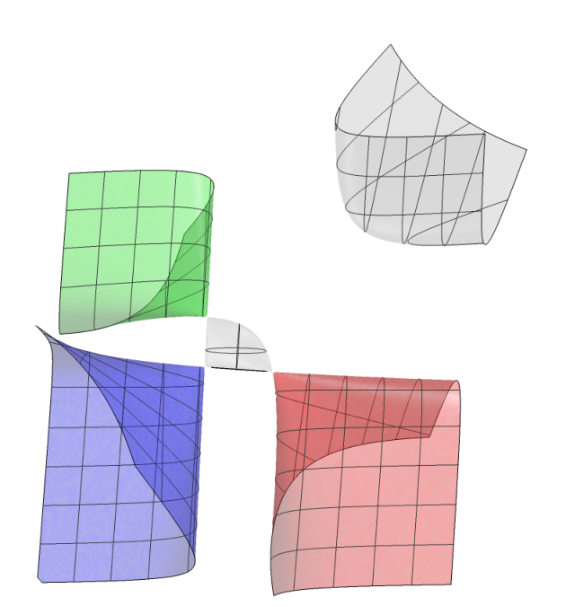
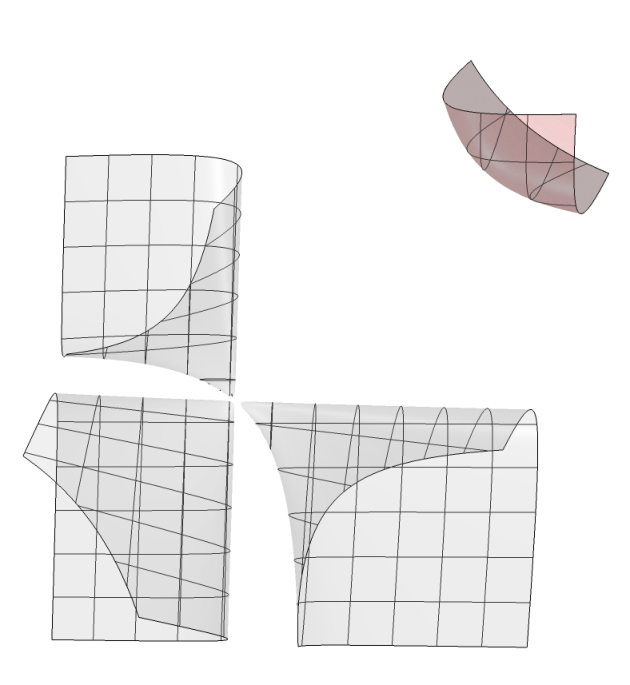
Refer to caption
Refer to caption
Refer to caption
Figure 4: Evolution of surfaces passing through a 33-step unipotent case.
Refer to caption
Refer to caption
Refer to caption
Refer to caption
Figure 5: Evolution of surfaces corresponding to real traces.

6 Relations of length 44: f-bendings and others

If we are to keep the conjugacy classes of the special elliptic isometries, bendings provide all nonorthogonal generic length 44 relations Rα2p2​Rα1p1=Rα2q2​Rα1q1R_{\alpha_{2}}^{p_{2}}R_{\alpha_{1}}^{p_{1}}=R_{\alpha_{2}}^{q_{2}}R_{\alpha_{1}}^{q_{1}} with δ=1\delta=1 and σ​pi=σ​qi\sigma p_{i}=\sigma q_{i} (see Theorem 4.7). Here, we describe all the remaining generic length 44 relations.

6.1. f-bendings

First, let us describe the nonorthogonal generic length 44 relations with δ=1\delta=1 and σ​pi=σ​qi\sigma p_{i}=\sigma q_{i} which are not bendings. Roughly speaking, they are constructed as follows: given a product Rα2p2​Rα1p1R_{\alpha_{2}}^{p_{2}}R_{\alpha_{1}}^{p_{1}}, we find a one-parameter family of products Rβ2​(t)q2​(t)​Rβ1​(t)q1​(t)R_{\beta_{2}(t)}^{q_{2}(t)}R_{\beta_{1}(t)}^{q_{1}(t)} acting on the line L⁡(p1,p2)\mathrm{L}(p_{1},p_{2}) as well as on its polar point in the same way as Rα2p2​Rα1p1R_{\alpha_{2}}^{p_{2}}R_{\alpha_{1}}^{p_{1}} does. As the next lemma shows, this in principle does not guarantee that we arrive at new length 44 relations; however, as we show in Proposition 6.6, a continuity argument settles the question.

6.2. Lemma.

Let R,S∈SU(2,1)R,S\in\mathop{\mathrm{SU}}(2,1) be isometries that stabilize a noneuclidean line L:=ℙ​c⊥L:=\mathbb{P}c^{\bot}. Suppose that the actions of RR and SS on LL coincide and that R​c=S​cRc=Sc (that is, cc is an eigenvector of same eigenvalue for both RR and SS). Then R=SR=S or R=R−1c​SR=R_{-1}^{c}S.

Proof. Assume that RR and SS are elliptic. Let λi\lambda_{i} and μi\mu_{i}, i=1,2,3i=1,2,3, be their respective eigenvalues with μ1=λ1\mu_{1}=\lambda_{1}. Let η∈ℂ\eta\in\mathbb{C}, |η|=1|\eta|=1, be such that η​λ2=μ2\eta\lambda_{2}=\mu_{2}. The fact that the actions of RR and SS on LL are the same implies that λ2​λ¯3=μ2​μ¯3\lambda_{2}\overline{\lambda}_{3}=\mu_{2}\overline{\mu}_{3}; hence, η​λ3=μ3\eta\lambda_{3}=\mu_{3}. Moreover, μ2​μ3=λ2​λ3\mu_{2}\mu_{3}=\lambda_{2}\lambda_{3} because R,S∈SU(2,1)R,S\in\mathop{\mathrm{SU}}(2,1). It follows that η=±1\eta=\pm 1 which concludes the proof in this case.

If RR and SS are loxodromic, we can write R=[λ−1​λ¯000λ000λ¯−1]R=\left[\begin{smallmatrix}\lambda^{-1}\overline{\lambda}&0&0\\ 0&\lambda&0\\ 0&0&\overline{\lambda}^{-1}\end{smallmatrix}\right] and S=[μ−1​μ¯000μ000μ¯−1]S=\left[\begin{smallmatrix}\mu^{-1}\overline{\mu}&0&0\\ 0&\mu&0\\ 0&0&\overline{\mu}^{-1}\end{smallmatrix}\right], where λ−1​λ¯\lambda^{-1}\overline{\lambda} and μ−1​μ¯\mu^{-1}\overline{\mu} are, respectively, the (equal) eigenvalues associated to cc. Let η∈ℂ\eta\in\mathbb{C} be such that η​λ=μ\eta\lambda=\mu. The fact that the actions of RR and SS on LL are the same implies that λ​λ¯=μ​μ¯\lambda\overline{\lambda}=\mu\overline{\mu}. So, |η|=1|\eta|=1. It now follows from λ−1​λ¯=μ−1​μ¯\lambda^{-1}\overline{\lambda}=\mu^{-1}\overline{\mu} that η=±1\eta=\pm 1.

Finally, assume that RR and SS are parabolic. Since RR and SS stabilize a noneuclidean complex line, neither of them can be 33-step unipotent (see Subsection 2.1). As in the proof of Proposition 4.3, we write R=[λ−2000λi​r​λ00λ]R=\left[\begin{smallmatrix}\lambda^{-2}&0&0\\ 0&\lambda&ir\lambda\\ 0&0&\lambda\end{smallmatrix}\right] and S=[μ−2000μi​s​μ00μ]S=\left[\begin{smallmatrix}\mu^{-2}&0&0\\ 0&\mu&is\mu\\ 0&0&\mu\end{smallmatrix}\right], where |λ|=1|\lambda|=1, |μ|=1|\mu|=1, r,s∈ℝr,s\in\mathbb{R}, and λ−2\lambda^{-2} and μ−2\mu^{-2} are, respectively, the (equal) eigenvalues related to cc. (The 22-step unipotent case corresponds to λ=1\lambda=1 or μ=1\mu=1.) Hence, μ=±λ\mu=\pm\lambda. The above matrices are written in a basis c,v1,v2c,v_{1},v_{2}, where v1,v2∈L∩S​Vv_{1},v_{2}\in L\cap{\mathrm{S}}\,V, v1≠v2v_{1}\neq v_{2}, and v1v_{1} is the isotropic fixed point of both RR and SS. The action of (say) RR on L∖{v2}L\setminus\{v_{2}\} is given by v1+τ​v2↦v1+(τ1+i​r​τ)​v2v_{1}+\tau v_{2}\mapsto v_{1}+\big(\frac{\tau}{1+ir\tau}\big)v_{2}. By hypothesis, RR and SS act in the same way on LL; so, r=sr=s.□\hfill\square

[Uncaptioned image]

x

6.3. Definition.

A relation Rα2p2​Rα1p1=Rβ2q2​Rβ1q1R_{\alpha_{2}}^{p_{2}}R_{\alpha_{1}}^{p_{1}}=R_{\beta_{2}}^{q_{2}}R_{\beta_{1}}^{q_{1}} is called an ff-bending if: (i) qi∈Giq_{i}\in G_{i}, i=1,2i=1,2, where G,G1,G2G,G_{1},G_{2} are geodesics associated to R:=Rα2p2​Rα1p1R:=R_{\alpha_{2}}^{p_{2}}R_{\alpha_{1}}^{p_{1}} (see Definition 4.6); (ii) σ​qi=σ​pi\sigma q_{i}=\sigma p_{i} and ⟨pi,qi⟩≠0\langle p_{i},q_{i}\rangle\neq 0, i=1,2i=1,2; (iii) α1​α2=β1​β2\alpha_{1}\alpha_{2}=\beta_{1}\beta_{2} and αi∼βi\alpha_{i}\sim\beta_{i} (see Definition 4.4); (iv) neither G⁡[p1,q1]\mathrm{G}[p_{1},q_{1}] nor G⁡[p2,q2]\mathrm{G}[p_{2},q_{2}] contains a fixed point of RR.

It is worthwhile observing that, when Rα2p2​Rα1p1=Rβ2q2​Rβ1q1R_{\alpha_{2}}^{p_{2}}R_{\alpha_{1}}^{p_{1}}=R_{\beta_{2}}^{q_{2}}R_{\beta_{1}}^{q_{1}} is an ff-bending relation, the condition qi∈Giq_{i}\in G_{i} implies Gi=HiG_{i}=H_{i}, where G,G1,G2G,G_{1},G_{2} and H,H1,H2H,H_{1},H_{2} are the geodesics respectively associated to R1:=Rα2p2​Rα1p1R_{1}:=R_{\alpha_{2}}^{p_{2}}R_{\alpha_{1}}^{p_{1}} and to R2:=Rβ2q2​Rβ1q1R_{2}:=R_{\beta_{2}}^{q_{2}}R_{\beta_{1}}^{q_{1}}.

In order to characterize ff-bendings in Proposition 6.6 and Theorem 6.5, we need the following simple lemma whose proof is straightforward.

6.4. Lemma.

Let αi,βi∈𝕊1∖Ω\alpha_{i},\beta_{i}\in\mathbb{S}^{1}\setminus\Omega with αi∼βi\alpha_{i}\sim\beta_{i} and let ai,bia_{i},b_{i} be the primitives of αi,βi\alpha_{i},\beta_{i}, i=1,2i=1,2 (see Definition 4.4). Then a1​a2=b1​b2a_{1}a_{2}=b_{1}b_{2} iff α1​α2=β1​β2\alpha_{1}\alpha_{2}=\beta_{1}\beta_{2}.

In what follows, we obtain ff-bending relations via a certain deformation. Such a deformation will be shown to exist in Theorem 6.5.

An ff-configuration consists of two tuples (p1,p2,α1,α2)(p_{1},p_{2},\alpha_{1},\alpha_{2}), (q1,q2,β1,β2)(q_{1},q_{2},\beta_{1},\beta_{2}) satisfying the following conditions: (i) p1,p2p_{1},p_{2} is a pair of distinct nonisotropic nonorthogonal points and the same holds for q1,q2q_{1},q_{2}; (ii) σ​pi=σ​qi\sigma p_{i}=\sigma q_{i} and ⟨pi,qi⟩≠0\langle p_{i},q_{i}\rangle\neq 0, i=1,2i=1,2; (iii) αi,βi∈𝕊1∖Ω\alpha_{i},\beta_{i}\in\mathbb{S}^{1}\setminus\Omega; (iv) Gi=HiG_{i}=H_{i}, ∠p1​G1​G=Arga13\angle_{p_{1}}G_{1}G=\mathop{\mathrm{Arg}}a_{1}^{3}, ∠p2​G​G2=Arga23\angle_{p_{2}}GG_{2}=\mathop{\mathrm{Arg}}a_{2}^{3}, ∠q1​G1​H=Argb13\angle_{q_{1}}G_{1}H=\mathop{\mathrm{Arg}}b_{1}^{3}, ∠q2​H​G2=Argb23\angle_{q_{2}}HG_{2}=\mathop{\mathrm{Arg}}b_{2}^{3}, where ai,bia_{i},b_{i} are the primitive angles of αi,βi\alpha_{i},\beta_{i} and G,G1,G2G,G_{1},G_{2} (respectively, H,H1,H2H,H_{1},H_{2}) are the geodesics associated to Rα2p2​Rα1p1R_{\alpha_{2}}^{p_{2}}R_{\alpha_{1}}^{p_{1}} (respectively, to Rβ2q2​Rβ1q1R_{\beta_{2}}^{q_{2}}R_{\beta_{1}}^{q_{1}}); and (v) neither G⁡[p1,q1]\mathrm{G}[p_{1},q_{1}] nor G⁡[p2,q2]\mathrm{G}[p_{2},q_{2}] contains an intersection point of G1,G2G_{1},G_{2}. In other words, an ff-configuration is essentially a pair of products R1:=Rα2p2​Rα1p1R_{1}:=R_{\alpha_{2}}^{p_{2}}R_{\alpha_{1}}^{p_{1}} and R2:=Rβ2q2​Rβ1q1R_{2}:=R_{\beta_{2}}^{q_{2}}R_{\beta_{1}}^{q_{1}} whose actions on L⁡(p1,p2)=L⁡(q1,q2)\mathrm{L}(p_{1},p_{2})=\mathrm{L}(q_{1},q_{2}) coincide and whose associated geodesics Gi,HiG_{i},H_{i} have been made equal after a bending.

Let (p1,p2,α1,α2)(p_{1},p_{2},\alpha_{1},\alpha_{2}), (q1,q2,β1,β2)(q_{1},q_{2},\beta_{1},\beta_{2}) be an ff-configuration. We take parameterizations γi:[a,b]→Gi\gamma_{i}:[a,b]\to G_{i} such that σ​γi​(t)=σ​pi\sigma\gamma_{i}(t)=\sigma p_{i} and ⟨γ1​(t),γ2​(t)⟩≠0\big\langle\gamma_{1}(t),\gamma_{2}(t)\big\rangle\neq 0 for all t∈[a,b]t\in[a,b]. Let hi=hi​(t)∈Jh_{i}=h_{i}(t)\in J be defined by ∠γ1​(t)​G1​G′=Argh1​(t)3\angle_{\gamma_{1}(t)}G_{1}G^{\prime}=\mathop{\mathrm{Arg}}h_{1}(t)^{3} and ∠γ2​(t)​G′​G2=Argh2​(t)3\angle_{\gamma_{2}(t)}G^{\prime}G_{2}=\mathop{\mathrm{Arg}}h_{2}(t)^{3}, where G′=Gt′:=G≀γ1(t),γ2(t)≀G^{\prime}=G^{\prime}_{t}:=\mathrm{G}{\wr}\gamma_{1}(t),\gamma_{2}(t){\wr}. Moreover, let ηi=ηi​(t)∈𝕊1\eta_{i}=\eta_{i}(t)\in\mathbb{S}^{1} be defined by ηi∼αi\eta_{i}\sim\alpha_{i} and ηi​(t)3=(hi​(t)2)3\eta_{i}(t)^{3}=(h_{i}(t)^{2})^{3}, t∈[a,b]t\in[a,b]. Hence, ηi​(t)\eta_{i}(t) is the parameter in the same component as αi\alpha_{i} whose primitive equals hi​(t)h_{i}(t).

We say that a given ff-configuration is ff-connected if there exist continuous parameterizations γi\gamma_{i} as above such that γi​(a)=pi\gamma_{i}(a)=p_{i}, γi​(b)=qi\gamma_{i}(b)=q_{i}, and η1​(t)​η2​(t)=α1​α2\eta_{1}(t)\eta_{2}(t)=\alpha_{1}\alpha_{2} for all t∈[a,b]t\in[a,b]. By Lemma 6.4, it is equivalent to require h1​(t)​h2​(t)=a1​a2h_{1}(t)h_{2}(t)=a_{1}a_{2} for all t∈[a,b]t\in[a,b]. Note that α1​α2=β1​β2\alpha_{1}\alpha_{2}=\beta_{1}\beta_{2} and αi∼βi\alpha_{i}\sim\beta_{i} if the ff-configuration is ff-connected. The converse also holds:

6.5. Theorem.

An ff-configuration (p1,p2,α1,α2)(p_{1},p_{2},\alpha_{1},\alpha_{2}), (q1,q2,β1,β2)(q_{1},q_{2},\beta_{1},\beta_{2}) is ff-connected iff α1​α2=β1​β2\alpha_{1}\alpha_{2}=\beta_{1}\beta_{2} and αi∼βi\alpha_{i}\sim\beta_{i}, i=1,2i=1,2.

Proof. We already know that ff-connectedness implies α1​α2=β1​β2\alpha_{1}\alpha_{2}=\beta_{1}\beta_{2} and αi∼βi\alpha_{i}\sim\beta_{i}. Assume that α1​α2=β1​β2\alpha_{1}\alpha_{2}=\beta_{1}\beta_{2} and αi∼βi\alpha_{i}\sim\beta_{i}. Clearly, we can assume pi≠qip_{i}\neq q_{i}, i=1,2i=1,2, since pi=qip_{i}=q_{i} is equivalent to αi=βi\alpha_{i}=\beta_{i}.

Suppose that σ​p1=σ​p2\sigma p_{1}=\sigma p_{2}. It follows from α1​α2=β1​β2\alpha_{1}\alpha_{2}=\beta_{1}\beta_{2} and Lemma 6.4 that A1+A2=B1+B2A_{1}+A_{2}=B_{1}+B_{2}, where Ai:=Argai3A_{i}:=\mathop{\mathrm{Arg}}a_{i}^{3}, Bi:=Argbi3B_{i}:=\mathop{\mathrm{Arg}}b_{i}^{3}, and ai,bia_{i},b_{i} are the respective primitives of αi,βi\alpha_{i},\beta_{i}. It is now easy to see that the geodesic segments G⁡[p1,p2]\mathrm{G}[p_{1},p_{2}] and G⁡[q1,q2]\mathrm{G}[q_{1},q_{2}] intersect at a point yy and that the triangles Δ⁡(p1,y,q1)\Delta(p_{1},y,q_{1}) and Δ⁡(q2,y,p2)\Delta(q_{2},y,p_{2}) have opposite orientations and the same area (see item (a) in the figure below).

Let γi:[0,ℓi]→G⁡[pi,qi]\gamma_{i}:[0,\ell_{i}]\to\mathrm{G}[p_{i},q_{i}] be the arc length parameterization of the geodesic segment G⁡[pi,qi]\mathrm{G}[p_{i},q_{i}], i=1,2i=1,2. Taking into account condition (v) in the definition of ff-configuration, it follows from simple considerations of plane hyperbolic (or, according to the nature of the projective line L⁡(p1,p2)\mathrm{L}(p_{1},p_{2}), of spherical) geometry that, given s∈[0,ℓ1]s\in[0,\ell_{1}], there exists a unique t=t⁡(s)∈[0,ℓ2]t=t(s)\in[0,\ell_{2}] such that the geodesic segments G⁡[p1,p2]\mathrm{G}[p_{1},p_{2}] and G⁡[γ1​(s),γ2​(t)]\mathrm{G}\big[\gamma_{1}(s),\gamma_{2}(t)\big] intersect at a point ysy_{s} and the triangles Δ⁡(p1,ys,γ1​(s))\Delta\big(p_{1},y_{s},\gamma_{1}(s)\big) and Δ⁡(γ2​(t),ys,p2)\Delta\big(\gamma_{2}(t),y_{s},p_{2}\big) have opposite orientations and the same area (see item (b) in the figure below). In this way, we obtain a strictly increasing bijection (therefore, continuous) [0,ℓ1]→[0,ℓ2][0,\ell_{1}]\to[0,\ell_{2}] which leads to a new parameterization γ2:[0,ℓ1]→G⁡[p2,q2]\gamma_{2}:[0,\ell_{1}]\to\mathrm{G}[p_{2},q_{2}]. Now, γ1,γ2\gamma_{1},\gamma_{2} satisfy the conditions in the definition of ff-connectedness because η1​(t)​η2​(t)=α1​α2\eta_{1}(t)\eta_{2}(t)=\alpha_{1}\alpha_{2} follows from an argument analogous to the one in the previous paragraph.

[Uncaptioned image]
[Uncaptioned image]
[Uncaptioned image]
[Uncaptioned image]

Suppose that σ​p1≠σ​p2\sigma p_{1}\neq\sigma p_{2} (in particular, L:=L⁡(p1,p2)L:=\mathrm{L}(p_{1},p_{2}) is hyperbolic) and take the points p~2,q~2∈L\tilde{p}_{2},\tilde{q}_{2}\in L orthogonal to p2,q2p_{2},q_{2}. Let us show that G⁡[p1,p~2]∩G⁡[q1,q~2]=∅\mathrm{G}[p_{1},\tilde{p}_{2}]\cap\mathrm{G}[q_{1},\tilde{q}_{2}]=\varnothing. Assume that the mentioned segments intersect at a point yy. The areas of the triangles Δ⁡(y,p1,q1)\Delta(y,p_{1},q_{1}) and Δ⁡(y,p~2,q~2)\Delta(y,\tilde{p}_{2},\tilde{q}_{2}) equal ±(A1−B1)−C>0\pm(A_{1}-B_{1})-C>0 and ±(A2−B2)−C>0\pm(A_{2}-B_{2})-C>0 (depending on the orientation of the triangles) where Ai,BiA_{i},B_{i} are defined as above and CC is the interior angle of the triangles at yy. It follows from Lemma 6.4 that A1+A2=B1+B2A_{1}+A_{2}=B_{1}+B_{2}; this leads to C<0C<0, a contradiction. Therefore, the quadrilateral of vertices p1,q1,q~2,p~2p_{1},q_{1},\tilde{q}_{2},\tilde{p}_{2} is simple and its oriented area equals ±2​(B1−A1)=±2​(A2−B2)\pm 2(B_{1}-A_{1})=\pm 2(A_{2}-B_{2}).

Assume Arga13<Argb13\mathop{\mathrm{Arg}}a_{1}^{3}<\mathop{\mathrm{Arg}}b_{1}^{3} and take [a,b]:=[Arga13,Argb13][a,b]:=[\mathop{\mathrm{Arg}}a_{1}^{3},\mathop{\mathrm{Arg}}b_{1}^{3}]. Let γ1:[0,ℓ1]→G⁡[p1,q1]\gamma_{1}:[0,\ell_{1}]\to\mathrm{G}[p_{1},q_{1}] and γ~2:[0,ℓ2]→G⁡[p~2,q~2]\tilde{\gamma}_{2}:[0,\ell_{2}]\to\mathrm{G}[\tilde{p}_{2},\tilde{q}_{2}] be arc length parameterizations. Given t∈[a,b]t\in[a,b], it follows from usual arguments in plane hyperbolic geometry that: (1) there exists unique s1=s1​(t)∈[0,ℓ1]s_{1}=s_{1}(t)\in[0,\ell_{1}], s2=s2​(t)∈[0,ℓ2]s_{2}=s_{2}(t)\in[0,\ell_{2}] such that the oriented area of the quadrilateral of vertices p1,γ1​(s1),γ~2​(s2),p~2p_{1},\gamma_{1}(s_{1}),\tilde{\gamma}_{2}(s_{2}),\tilde{p}_{2} equals ±2​(A1−t)\pm 2(A_{1}-t) (in order to see this, consider the geodesic Γt,s\Gamma_{t,s} through the point γ1​(s)\gamma_{1}(s) such that ∠γ1​(s)​G1​Γt,s=t\angle_{\gamma_{1}(s)}G_{1}\Gamma_{t,s}=t and vary s∈[0,ℓ1]s\in[0,\ell_{1}]); (2) the bijections t↦si​(t)t\mapsto s_{i}(t), i=1,2i=1,2, are strictly increasing (hence, continuous). We obtain new parameterizations γ1:[a,b]→G⁡[p1,q1]\gamma_{1}:[a,b]\to\mathrm{G}[p_{1},q_{1}] and γ~2:[a,b]→G⁡[p~2,q~2]\tilde{\gamma}_{2}:[a,b]\to\mathrm{G}[\tilde{p}_{2},\tilde{q}_{2}] that imply the ff-connectedness of the ff-configurations in question because Area(p1,γ1​(s1),γ~2​(s2),p~2)=±2​(A1−t)\mathop{\mathrm{Area}}\big(p_{1},\gamma_{1}(s_{1}),\tilde{\gamma}_{2}(s_{2}),\tilde{p}_{2}\big)=\pm 2(A_{1}-t) is equivalent to η1​(t)​η2​(t)=α1​α2\eta_{1}(t)\eta_{2}(t)=\alpha_{1}\alpha_{2}, where Area(p1,γ1​(s1),γ~2​(s2),p~2)\mathop{\mathrm{Area}}\big(p_{1},\gamma_{1}(s_{1}),\tilde{\gamma}_{2}(s_{2}),\tilde{p}_{2}\big) denotes the oriented area of the oriented quadrilateral of vertices p1,γ1​(s1),γ~2​(s2),p~2p_{1},\gamma_{1}(s_{1}),\tilde{\gamma}_{2}(s_{2}),\tilde{p}_{2}.□\hfill\square

6.6. Proposition.

An ff-configuration (p1,p2,α1,α2),(q1,q2,β1,β2)(p_{1},p_{2},\alpha_{1},\alpha_{2}),(q_{1},q_{2},\beta_{1},\beta_{2}) is ff-connected iff Rα2p2​Rα1p1=Rβ2q2​Rβ1q1R_{\alpha_{2}}^{p_{2}}R_{\alpha_{1}}^{p_{1}}=R_{\beta_{2}}^{q_{2}}R_{\beta_{1}}^{q_{1}} is an ff-bending relation.

Proof.

If Rα2p2​Rα1p1=Rβ2q2​Rβ1q1R_{\alpha_{2}}^{p_{2}}R_{\alpha_{1}}^{p_{1}}=R_{\beta_{2}}^{q_{2}}R_{\beta_{1}}^{q_{1}} is an ff-bending relation, one can readily see that (p1,p2,α1,α2)(p_{1},p_{2},\alpha_{1},\alpha_{2}), (q1,q2,β1,β2)(q_{1},q_{2},\beta_{1},\beta_{2}) is an ff-configuration with α1​α2=β1​β2\alpha_{1}\alpha_{2}=\beta_{1}\beta_{2} and αi∼βi\alpha_{i}\sim\beta_{i}. It follows from Theorem 6.5 that the ff-configuration is ff-connected. Conversely, let γi:[a,b]→G⁡[pi,qi]\gamma_{i}:[a,b]\to\mathrm{G}[p_{i},q_{i}], be the parameterizations associated to the ff-connectedness of the ff-configuration. By construction, Gt′,G1,G2G^{\prime}_{t},G_{1},G_{2}, where Gt′:=G≀γ1(t),γ2(t)≀G^{\prime}_{t}:=\mathrm{G}{\wr}\gamma_{1}(t),\gamma_{2}(t){\wr}, are the geodesics associated to S=S⁡(t):=Rη2​(t)γ2​(t)​Rη1​(t)γ1​(t)S=S(t):=R_{\eta_{2}(t)}^{\gamma_{2}(t)}R_{\eta_{1}(t)}^{\gamma_{1}(t)} (see the above definition of ff-connectedness for the definition of the functions ηi\eta_{i}). Lemma 4.5 implies that the actions of R:=Rα2p2​Rα1p1R:=R_{\alpha_{2}}^{p_{2}}R_{\alpha_{1}}^{p_{1}} and of SS on L:=L⁡(p1,p2)L:=\mathrm{L}(p_{1},p_{2}) coincide. Furthermore, it follows from η1​(t)​η2​(t)=α1​α2\eta_{1}(t)\eta_{2}(t)=\alpha_{1}\alpha_{2} that R​c=S⁡(t)​cRc=S(t)c, where cc is the polar point of LL. So, by Lemma 6.2 and by continuity, either R=S⁡(t)R=S(t) or R=R−1c​S​(t)R=R_{-1}^{c}S(t) for all tt. It remains to take t=a,bt=a,b. ∎

In view of Theorem 6.5, it is natural to ask the following. Given a product Rα2p2​Rα1p1R_{\alpha_{2}}^{p_{2}}R_{\alpha_{1}}^{p_{1}} and parameters βi∈𝕊1∖Ω\beta_{i}\in\mathbb{S}^{1}\setminus\Omega satisfying α1​α2=β1​β2\alpha_{1}\alpha_{2}=\beta_{1}\beta_{2} and αi∼βi\alpha_{i}\sim\beta_{i}, do there exist qi∈Giq_{i}\in G_{i}, σ​qi=σ​pi\sigma q_{i}=\sigma p_{i}, such that Rα2p2​Rα1p1=Rβ2q2​Rβ1q1R_{\alpha_{2}}^{p_{2}}R_{\alpha_{1}}^{p_{1}}=R_{\beta_{2}}^{q_{2}}R_{\beta_{1}}^{q_{1}}? The answer is affirmative at least in the particular cases dealt with in the next couple of propositions.

6.7. Proposition.

Let pi∈ℙ​V∖S​Vp_{i}\in\mathbb{P}V\setminus{\mathrm{S}}\,V be distinct nonorthogonal points of the same signature such that L⁡(p1,p2)\mathrm{L}(p_{1},p_{2}) is hyperbolic and let αi,βi∈𝕊1∖Ω\alpha_{i},\beta_{i}\in\mathbb{S}^{1}\setminus\Omega be parameters, i=1,2i=1,2. Assume that α1​α2=β1​β2\alpha_{1}\alpha_{2}=\beta_{1}\beta_{2} and αi∼βi\alpha_{i}\sim\beta_{i}, i=1,2i=1,2. There exists an ff-bending relation Rα2p2​Rα1p1=Rβ2q2​Rβ1q1R_{\alpha_{2}}^{p_{2}}R_{\alpha_{1}}^{p_{1}}=R_{\beta_{2}}^{q_{2}}R_{\beta_{1}}^{q_{1}}.

Proof.

Let ai,bia_{i},b_{i} be the primitives of αi,βi\alpha_{i},\beta_{i}. We divide the proof in two cases:

(1) Arg(a1​a2)3⩽π\mathop{\mathrm{Arg}}(a_{1}a_{2})^{3}\leqslant\pi, or, equivalently, a1​a2a_{1}a_{2} lie in the arc (1,−ω2](1,-\omega^{2}] (if Arg(a1​a2)3=0\mathop{\mathrm{Arg}}(a_{1}a_{2})^{3}=0, then a1=a2=−ω2a_{1}=a_{2}=-\omega^{2})

(2) Arg(a1​a2)3>π\mathop{\mathrm{Arg}}(a_{1}a_{2})^{3}>\pi, or, equivalently, a1​a2a_{1}a_{2} lie in the arc (−ω2,ω)(-\omega^{2},\omega).

Assume that the first case holds. Proceeding as in the proof of Theorem 6.5, we continuously move the point pip_{i} along GiG_{i}. Abusing notation, we denote the new obtained points by qiq_{i} and new corresponding parameters by ηi\eta_{i}. The deformation is performed in such a way that the ff-configurations (p1,p2,α1,α2),(q1,q2,η1,η2)(p_{1},p_{2},\alpha_{1},\alpha_{2}),(q_{1},q_{2},\eta_{1},\eta_{2}) are ff-connected. Due to a1a2∈arc(1,−ω2]a_{1}a_{2}\in\mathop{\mathrm{arc}}(1,-\omega^{2}], sending q1q_{1} to the absolute makes the angle Argh13\mathop{\mathrm{Arg}}h_{1}^{3} as small as desired; here, hih_{i} stands for the primitive of ηi\eta_{i}. So, h1h_{1} assumes every value in arc(1,a1)\mathop{\mathrm{arc}}(1,a_{1}). Since h1​h2=a1​a2h_{1}h_{2}=a_{1}a_{2} during the deformation, h2h_{2} assumes every value in arc(a2,a1​a2)\mathop{\mathrm{arc}}(a_{2},a_{1}a_{2}) (and the point q2q_{2} tends to some limit point in G2G_{2}). Changing the roles of q1,q2q_{1},q_{2} in the deformation, that is, sending q2q_{2} to the absolute, we can see that there exists q1,q2q_{1},q_{2} corresponding to every value of h1h_{1} in the arc (1,a1​a2)(1,a_{1}a_{2}). Since α1​α2=β1​β2\alpha_{1}\alpha_{2}=\beta_{1}\beta_{2} and αi∼βi\alpha_{i}\sim\beta_{i}, Lemma 6.4 implies that a1​a2=b1​b2a_{1}a_{2}=b_{1}b_{2} and, therefore, b1,b2∈arc(1,a1​a2)b_{1},b_{2}\in\mathop{\mathrm{arc}}(1,a_{1}a_{2}). It remains to take h1=b1h_{1}=b_{1} (which implies OPENh2=b2)h_{2}=b_{2}): the corresponding q1,q2q_{1},q_{2} are the points we are looking for.

The second case is similar. Sending q1q_{1} to the absolute makes the angle Argh13\mathop{\mathrm{Arg}}h_{1}^{3} tend to π\pi and, consequently, h1h_{1} assumes every value in arc(a1,−ω2)\mathop{\mathrm{arc}}(a_{1},-\omega^{2}); correspondingly, h2h_{2} assumes every value in arc(−ω​a1​a2,a2)\mathop{\mathrm{arc}}(-\omega a_{1}a_{2},a_{2}). So, there exist q1,q2q_{1},q_{2} corresponding to every value of h1h_{1} in arc(−ω​a1​a2,−ω2)\mathop{\mathrm{arc}}(-\omega a_{1}a_{2},-\omega^{2}). Again, a1​a2=b1​b2a_{1}a_{2}=b_{1}b_{2} implies that b1∈arc(−ω​a1​a2,−ω2)b_{1}\in\mathop{\mathrm{arc}}(-\omega a_{1}a_{2},-\omega^{2}). ∎

6.8. Proposition.

Let p1,p2∈ℙ​V∖S​Vp_{1},p_{2}\in\mathbb{P}V\setminus{\mathrm{S}}\,V be distinct nonorthogonal points of distinct signatures, σ​p1≠σ​p2\sigma p_{1}\neq\sigma p_{2}, and let α1,α2∈𝕊1∖Ω\alpha_{1},\alpha_{2}\in\mathbb{S}^{1}\setminus\Omega be such that Rα2p2​Rα1p1R_{\alpha_{2}}^{p_{2}}R_{\alpha_{1}}^{p_{1}} is loxodromic. Let β1,β2∈𝕊1\beta_{1},\beta_{2}\in\mathbb{S}^{1} be parameters satisfying α1​α2=β1​β2\alpha_{1}\alpha_{2}=\beta_{1}\beta_{2} and αi∼βi\alpha_{i}\sim\beta_{i}, i=1,2i=1,2. There exists an ff-bending relation Rα2p2​Rα1p1=Rβ2q2​Rβ1q1R_{\alpha_{2}}^{p_{2}}R_{\alpha_{1}}^{p_{1}}=R_{\beta_{2}}^{q_{2}}R_{\beta_{1}}^{q_{1}}.

Proof.

The proof is a direct adaptation of that of Proposition 6.7. The only change that is needed is to replace the deformation to the appropriate one describe in the proof of Theorem 6.5. ∎

6.9. Remark.

In the conditions of Propositions 6.7 or 6.8, there always exist an ff-bending relation Rα2p2​Rα1p1=Rβ2q2​Rβ1q1R_{\alpha_{2}}^{p_{2}}R_{\alpha_{1}}^{p_{1}}=R_{\beta_{2}}^{q_{2}}R_{\beta_{1}}^{q_{1}} such that the primitives of β1\beta_{1} and β2\beta_{2} are the same, i.e., β1=δ​β2\beta_{1}=\delta\beta_{2}, δ∈Ω\delta\in\Omega (this is a direct consequence of the corresponding proofs). Moreover, when p1,p2∈ℙ​Vp_{1},p_{2}\in\mathbb{P}V are distinct nonorthogonal points such that L⁡(p1,p2)\mathrm{L}(p_{1},p_{2}) is spherical, and given parameters α1,α2∈𝕊1∖Ω\alpha_{1},\alpha_{2}\in\mathbb{S}^{1}\setminus\Omega, it is easy to see that there exists an ff-bending relation Rα2p2​Rα1p1=Rβ2q2​Rβ1q1R_{\alpha_{2}}^{p_{2}}R_{\alpha_{1}}^{p_{1}}=R_{\beta_{2}}^{q_{2}}R_{\beta_{1}}^{q_{1}} such that the primitives of β1\beta_{1} and β2\beta_{2} are the same.

6.10. Remark.

Let α1,α2∈𝕊1∖Ω\alpha_{1},\alpha_{2}\in\mathbb{S}^{1}\setminus\Omega be parameters and let p1,p2∈ℙ​V∖S​Vp_{1},p_{2}\in\mathbb{P}V\setminus{\mathrm{S}}\,V be distinct nonisotropic nonorthogonal points. Assume that σ​p1=σ​p2\sigma p_{1}=\sigma p_{2} with L⁡(p1,p2)\mathrm{L}(p_{1},p_{2}) hyperbolic or that Rα2p2​Rα1p1R_{\alpha_{2}}^{p_{2}}R_{\alpha_{1}}^{p_{1}} is loxodromic. Let Ij=arc(ωj−1,ωj)I_{j}=\mathop{\mathrm{arc}}(\omega^{j-1},\omega^{j}) be the component of α1\alpha_{1} and let δ∈Ω\delta\in\Omega be such that δ⁡(α1​α2)∈Ij\delta(\alpha_{1}\alpha_{2})\in I_{j}. Among the arcs arc(ωj−1,δ⁡(α1​α2))\mathop{\mathrm{arc}}\big(\omega^{j-1},\delta(\alpha_{1}\alpha_{2})\big) and arc(δ⁡(α1​α2),ωj)\mathop{\mathrm{arc}}\big(\delta(\alpha_{1}\alpha_{2}),\omega^{j}\big), let Ij0I_{j}^{0} be the one containing α1\alpha_{1}. A corollary to the proof of Proposition 6.7 is that, by ff-bending Rα2p2​Rα1p1R_{\alpha_{2}}^{p_{2}}R_{\alpha_{1}}^{p_{1}}, it is possible to vary α1\alpha_{1} inside the entire Ij0I_{j}^{0}.

We can now give a description of all nonorthogonal generic length 44 relations in terms of bendings and ff-bendings (there is actually a nongeneric requirement on the signatures of points; the remaining case is dealt with in Subsection 6.12).

6.11. Theorem.

Let p1,p2p_{1},p_{2} and q1,q2q_{1},q_{2} be pairs of distinct nonisotropic nonorthogonal points with σ​pi=σ​qi\sigma p_{i}=\sigma q_{i} and let αi,βi∈𝕊1∖Ω\alpha_{i},\beta_{i}\in\mathbb{S}^{1}\setminus\Omega be parameters, αi∼βi\alpha_{i}\sim\beta_{i}, i=1,2i=1,2. Assume that L⁡(p1,p2)\mathrm{L}(p_{1},p_{2}) and L⁡(q1,q2)\mathrm{L}(q_{1},q_{2}) are noneuclidean and nonorthogonal. A length 44 relation Rα2p2​Rα1p1=Rβ2q2​Rβ1q1R_{\alpha_{2}}^{p_{2}}R_{\alpha_{1}}^{p_{1}}=R_{\beta_{2}}^{q_{2}}R_{\beta_{1}}^{q_{1}} follows from bending and ff-bending relations.

Proof.

Let G,G1,G2G,G_{1},G_{2} and H,H1,H2H,H_{1},H_{2} be the geodesics associated to Rα2p2​Rα1p1R_{\alpha_{2}}^{p_{2}}R_{\alpha_{1}}^{p_{1}} and Rβ2q2​Rβ1q1R_{\beta_{2}}^{q_{2}}R_{\beta_{1}}^{q_{1}}, respectively. By Lemma 4.1, we have L:=L⁡(p1,p2)=L⁡(q1,q2)L:=\mathrm{L}(p_{1},p_{2})=\mathrm{L}(q_{1},q_{2}) and α1​α2=β1​β2\alpha_{1}\alpha_{2}=\beta_{1}\beta_{2}. Bending q1,q2q_{1},q_{2} (if necessary), we make Gi=HiG_{i}=H_{i}.

Assume that LL is hyperbolic. It follows from α1​α2=β1​β2\alpha_{1}\alpha_{2}=\beta_{1}\beta_{2} that A1+A2=B1+B2A_{1}+A_{2}=B_{1}+B_{2}, where A1=∠p1​G1​GA_{1}=\angle_{p_{1}}G_{1}G, A2=∠p2​G​G2A_{2}=\angle_{p_{2}}GG_{2}, B1=∠q1​G1​HB_{1}=\angle_{q_{1}}G_{1}H, A2=∠q2​H​G2A_{2}=\angle_{q_{2}}HG_{2}. Now, proceeding as in the proof of Theorem 4.7, we can see that the previous bending can be made in a such a way that there is no fixed point of R:=Rα2p2​Rα1p1R:=R_{\alpha_{2}}^{p_{2}}R_{\alpha_{1}}^{p_{1}} neither in G⁡[p1,q1]\mathrm{G}[p_{1},q_{1}] nor in G⁡[p2,q2]\mathrm{G}[p_{2},q_{2}]. We just arrived at an ff-bending relation.

Suppose that LL is spherical. If the orientations of the triangles Δ⁡(x,p1,p2)\Delta(x,p_{1},p_{2}) and Δ⁡(x,q1,q2)\Delta(x,q_{1},q_{2}), where xx is a fixed point of RR, are the same, then the above bending can be made in such a way that we obtain an ff-bending relation. So, assume that the triangles have opposite orientations. By Remark 6.9, we can assume A1=A2A_{1}=A_{2} and B1=B2B_{1}=B_{2} modulo ff-bendings. It follows from α1​α2=β1​β2\alpha_{1}\alpha_{2}=\beta_{1}\beta_{2} that A1=A2=B1=B2A_{1}=A_{2}=B_{1}=B_{2} and can now proceed as in the proof of Theorem 4.7. ∎

6.12. Other length 4 relations

In what follows, we introduce and discuss the remaining length 44 relations. The nonorthogonal ones come in four flavours: changes of orientation, changes of components, simultaneous changes of signs, and single changes of sign.

Let p1,p2p_{1},p_{2} be distinct nonisotropic nonorthogonal points with noneuclidean L⁡(p1,p2)\mathrm{L}(p_{1},p_{2}) and let α1,α2∈𝕊1∖Ω\alpha_{1},\alpha_{2}\in\mathbb{S}^{1}\setminus\Omega. Note that

Rα2p2​Rα1p1=Rα2p2​Rα1p1​Rα¯2p2​Rα2p2=Rα1Rα2p2​p1​Rα2p2,R_{\alpha_{2}}^{p_{2}}R_{\alpha_{1}}^{p_{1}}=R_{\alpha_{2}}^{p_{2}}R_{\alpha_{1}}^{p_{1}}R_{\overline{\alpha}_{2}}^{p_{2}}R_{\alpha_{2}}^{p_{2}}=R_{\alpha_{1}}^{R_{\alpha_{2}}^{p_{2}}p_{1}}R_{\alpha_{2}}^{p_{2}},

where we are using a cancellation (see Definition 3.2) in the first equality. We arrive at the following definition.

6.13. Definition.

In the conditions above, the relation Rα2p2​Rα1p1=Rα1Rα2p2​p1​Rα2p2R_{\alpha_{2}}^{p_{2}}R_{\alpha_{1}}^{p_{1}}=R_{\alpha_{1}}^{R_{\alpha_{2}}^{p_{2}}p_{1}}R_{\alpha_{2}}^{p_{2}} is called a change of orientation.

6.14. Definition.

The relations Rα2p2​Rα1p1=Rω​α2p2​Rω−1​α1p1=Rω−1​α2p2​Rω​α1p1R_{\alpha_{2}}^{p_{2}}R_{\alpha_{1}}^{p_{1}}=R_{\omega\alpha_{2}}^{p_{2}}R_{\omega^{-1}\alpha_{1}}^{p_{1}}=R_{\omega^{-1}\alpha_{2}}^{p_{2}}R_{\omega\alpha_{1}}^{p_{1}} are called changes of components, where ω=e2​π​i/3\omega=e^{2\pi i/3}.

A change of components simultaneously changes the arcs IjI_{j}, j=0,1,2j=0,1,2, to which the parameters α1,α2\alpha_{1},\alpha_{2} belong (see Definition 4.4).

6.15. Proposition.

Let p1,p2p_{1},p_{2} and q1,q2q_{1},q_{2} be pairs of distinct nonisotropic nonorthogonal points and let α1,α2∈𝕊1∖Ω\alpha_{1},\alpha_{2}\in\mathbb{S}^{1}\setminus\Omega be parameters. Assume that σ​pi=−σ​qi\sigma p_{i}=-\sigma q_{i}, i=1,2i=1,2, and that ta(p1,p2)=ta(q1,q2)\mathop{\mathrm{ta}}(p_{1},p_{2})=\mathop{\mathrm{ta}}(q_{1},q_{2}) (in particular, L⁡(p1,p2)\mathrm{L}(p_{1},p_{2}) is hyperbolic). The isometries R1:=Rα2p2​Rα1p1R_{1}:=R_{\alpha_{2}}^{p_{2}}R_{\alpha_{1}}^{p_{1}} and R2:=Rα2q2​Rα1q1R_{2}:=R_{\alpha_{2}}^{q_{2}}R_{\alpha_{1}}^{q_{1}} are in the same conjugacy class iff they are not regular elliptic.

Proof.

By Remark 2.3, trR1=trR2\mathop{\mathrm{tr}}R_{1}=\mathop{\mathrm{tr}}R_{2} and, by Lemma 4.2, R1,R2R_{1},R_{2} are regular. Therefore, these isometries have the same type. If R1,R2R_{1},R_{2} are not regular elliptic, they are conjugate (see Subsection 2.1).

Conversely, suppose that R1,R2R_{1},R_{2} are regular elliptic. Using orthogonal relations of length 33 plus the fact that special elliptic isometries with orthogonal centres commute, we have

Rα1p~1​Rα2p~2​(Rα2p2​Rα1p1)​Rα¯2p~2​Rα¯1p~1=Rα1p~1​Rα¯2c​Rα1p1​Rα¯2p~2​Rα¯1p~1=Rα¯1c​Rα¯2c​Rα¯2p~2​Rα¯1p~1=Rα2p2​Rα1p1,R_{\alpha_{1}}^{\tilde{p}_{1}}R_{\alpha_{2}}^{\tilde{p}_{2}}(R_{\alpha_{2}}^{p_{2}}R_{\alpha_{1}}^{p_{1}})R_{\overline{\alpha}_{2}}^{\tilde{p}_{2}}R_{\overline{\alpha}_{1}}^{\tilde{p}_{1}}=R_{\alpha_{1}}^{\tilde{p}_{1}}R_{\overline{\alpha}_{2}}^{c}R_{\alpha_{1}}^{p_{1}}R_{\overline{\alpha}_{2}}^{\tilde{p}_{2}}R_{\overline{\alpha}_{1}}^{\tilde{p}_{1}}=R_{\overline{\alpha}_{1}}^{c}R_{\overline{\alpha}_{2}}^{c}R_{\overline{\alpha}_{2}}^{\tilde{p}_{2}}R_{\overline{\alpha}_{1}}^{\tilde{p}_{1}}=R_{\alpha_{2}}^{p_{2}}R_{\alpha_{1}}^{p_{1}},

where p~i\tilde{p}_{i} stands for the point in L:=L⁡(p1,p2)L:=\mathrm{L}(p_{1},p_{2}) orthogonal to pip_{i}. In other words, R~1:=Rα1p~1​Rα2p~2\widetilde{R}_{1}:=R_{\alpha_{1}}^{\tilde{p}_{1}}R_{\alpha_{2}}^{\tilde{p}_{2}} commutes with R1R_{1}. Since ta(p~1,p~2)=ta(p1,p2)\mathop{\mathrm{ta}}(\tilde{p}_{1},\tilde{p}_{2})=\mathop{\mathrm{ta}}(p_{1},p_{2}), the isometry R~1\widetilde{R}_{1} is regular elliptic and, by [8, Corollary 8.2], ⁡f​i​x​R~1=⁡f​i​x​R1\mathop{\mathrm{}}{fix}\widetilde{R}_{1}=\mathop{\mathrm{}}{fix}R_{1}. Hence, if R1,R~1R_{1},\widetilde{R}_{1} are conjugate, their actions on LL must coincide. Let G,G1,G2G,G_{1},G_{2} be the geodesics associated to R1R_{1} and let G~,G~1,G~2\widetilde{G},\widetilde{G}_{1},\widetilde{G}_{2} be the geodesics associated to R~1\widetilde{R}_{1}. Clearly, G~=G\widetilde{G}=G, G~1=G2\widetilde{G}_{1}=G_{2}, and G~2=G1\widetilde{G}_{2}=G_{1}. By Lemma 4.5, the actions of R1R_{1} and of R~1\widetilde{R}_{1} on L∩B​VL\cap{\mathrm{B}}\,V are respectively given by the products r2​r1r_{2}r_{1} and r1​r2r_{1}r_{2}, where rir_{i} denotes the reflection in the geodesic GiG_{i}. This implies that the actions of R1,R~1R_{1},\widetilde{R}_{1} coincide on LL iff ∠x​G1​G2=∠x​G2​G1=π2\angle_{x}G_{1}G_{2}=\angle_{x}G_{2}G_{1}=\frac{\pi}{2}, where x∈B​Vx\in{\mathrm{B}}\,V stands for the intersection of G1,G2G_{1},G_{2}, a fixed point of both isometries.

Assume ∠x​G2​G1=π2\angle_{x}G_{2}G_{1}=\frac{\pi}{2}. Let γ:(−a,a)→G\gamma:(-a,a)\to G be a parameterization of an open geodesic segment such that γ⁡(0)=p2\gamma(0)=p_{2}. Let R⁡(t):=Rα2γ⁡(t)​Rα1p1R(t):=R_{\alpha_{2}}^{\gamma(t)}R_{\alpha_{1}}^{p_{1}}; we can suppose that R⁡(t)R(t) is regular elliptic for all tt. Let G,G1,G2​(t)G,G_{1},G_{2}(t) be the geodesics associated to R⁡(t)R(t) and note that ∠γ⁡(t)​G​G2​(t)=∠p2​G​G2\angle_{\gamma(t)}GG_{2}(t)=\angle_{p_{2}}GG_{2}; so, ∠x⁡(t)​G2​G1=π2\angle_{x(t)}G_{2}G_{1}=\frac{\pi}{2} iff t=0t=0. Let x​(t),x~​(t)x(t),\tilde{x}(t) be respectively the negative and the positive intersections of G1G_{1} and G2​(t)G_{2}(t). Hence, x⁡(0)=xx(0)=x and x~​(0)=x~\tilde{x}(0)=\tilde{x} (clearly, x~​(t)\tilde{x}(t) is the orthogonal to x⁡(t)x(t) in LL for all tt). We denote by λ1​(t),λ2​(t)\lambda_{1}(t),\lambda_{2}(t) the eigenvalues of R⁡(t)R(t) corresponding to the eigenvectors x​(t),x~​(t)x(t),\tilde{x}(t). It is easy to see that λi​(t)\lambda_{i}(t) varies continuously with tt. Moreover, by Lemma 4.2, λ1​(t)≠λ2​(t)\lambda_{1}(t)\neq\lambda_{2}(t) for all tt.

Consider the isometry R~​(t):=Rα1p~1​Rα2γ~​(t)\widetilde{R}(t):=R_{\alpha_{1}}^{\tilde{p}_{1}}R_{\alpha_{2}}^{\tilde{\gamma}(t)}, t∈(−a,a)t\in(-a,a), where γ~​(t)\tilde{\gamma}(t) stands for the orthogonal to γ⁡(t)\gamma(t) in LL for all tt. As above, R~​(t)\widetilde{R}(t) and R⁡(t)R(t) have the same set of eigenvalues and ⁡f​i​x​R~​(t)=⁡f​i​x​R​(t)\mathop{\mathrm{}}{fix}\widetilde{R}(t)=\mathop{\mathrm{}}{fix}R(t). Hence, by the argument in the previous paragraph, we obtain that, for all t≠0t\neq 0, the isometries R⁡(t)R(t) and R~​(t)\widetilde{R}(t) are not conjugate due to ∠x⁡(t)​G2​G1≠π2\angle_{x(t)}G_{2}G_{1}\neq\frac{\pi}{2} for t≠0t\neq 0. In other words, λ2​(t)\lambda_{2}(t) must be the eigenvalue of R~​(t)\widetilde{R}(t) corresponding to x⁡(t)x(t). By continuity, the eigenvalues of the negative fixed point xx of R=R⁡(0)R=R(0) and of R~=R~​(0)\widetilde{R}=\widetilde{R}(0) are distinct and, therefore, these isometries cannot be conjugate. (We have λ1​(0)=−λ2​(0)\lambda_{1}(0)=-\lambda_{2}(0), as it is easy to see.)

Let I∈SU(2,1)I\in\mathop{\mathrm{SU}}(2,1) be such that I​qi=p~iIq_{i}=\tilde{p}_{i}. Thus I​Rα2q2​Rα1q1​I−1=Rα2p~2​Rα1p~1IR_{\alpha_{2}}^{q_{2}}R_{\alpha_{1}}^{q_{1}}I^{-1}=R_{\alpha_{2}}^{\tilde{p}_{2}}R_{\alpha_{1}}^{\tilde{p}_{1}}. Also note that

Rα¯2p~2​(Rα2p~2​Rα1p~1)​Rα2p~2=Rα1p~1​Rα2p~2.R_{\overline{\alpha}_{2}}^{\tilde{p}_{2}}\big(R_{\alpha_{2}}^{\tilde{p}_{2}}R_{\alpha_{1}}^{\tilde{p}_{1}}\big)R_{\alpha_{2}}^{\tilde{p}_{2}}=R_{\alpha_{1}}^{\tilde{p}_{1}}R_{\alpha_{2}}^{\tilde{p}_{2}}. (17)

Therefore, Rα2q2​Rα1q1R_{\alpha_{2}}^{q_{2}}R_{\alpha_{1}}^{q_{1}} and Rα1p~1​Rα2p~2R_{\alpha_{1}}^{\tilde{p}_{1}}R_{\alpha_{2}}^{\tilde{p}_{2}} are in the same conjugacy class, which is not that of Rα2p2​Rα1p1R_{\alpha_{2}}^{p_{2}}R_{\alpha_{1}}^{p_{1}}. ∎

6.16. Definition.

Let p1,p2p_{1},p_{2} and q1,q2q_{1},q_{2} be pairs of distinct nonisotropic nonorthogonal points with σ​pi=−σ​qi\sigma p_{i}=-\sigma q_{i} and ta(p1,p2)=ta(q1,q2)\mathop{\mathrm{ta}}(p_{1},p_{2})=\mathop{\mathrm{ta}}(q_{1},q_{2}). Let α1,α2∈𝕊1∖Ω\alpha_{1},\alpha_{2}\in\mathbb{S}^{1}\setminus\Omega be parameters and assume that Rα2p2​Rα1p1R_{\alpha_{2}}^{p_{2}}R_{\alpha_{1}}^{p_{1}} is not regular elliptic. Let I∈SU(2,1)I\in\mathop{\mathrm{SU}}(2,1) be such that Rα2p2​Rα1p1=I​Rα2q2​Rα1q1​I−1=Rα2I​q2​Rα1I​q1R_{\alpha_{2}}^{p_{2}}R_{\alpha_{1}}^{p_{1}}=IR_{\alpha_{2}}^{q_{2}}R_{\alpha_{1}}^{q_{1}}I^{-1}=R_{\alpha_{2}}^{Iq_{2}}R_{\alpha_{1}}^{Iq_{1}}. We call such relations simultaneous changes of signs and their existence is a consequence of Proposition 6.15. Note that, by Lemma 4.1, p1,p2,I​q1,I​q2p_{1},p_{2},Iq_{1},Iq_{2} lie in the same complex line.

[Uncaptioned image]

Given parameters α1,α2∈𝕊1∖Ω\alpha_{1},\alpha_{2}\in\mathbb{S}^{1}\setminus\Omega, define τα1,α2:ℝ→ℂ\tau_{\alpha_{1},\alpha_{2}}:\mathbb{R}\to\mathbb{C},

τα1,α2​(t):=α1​α2+α1−2​α2+α1​α2−2+(α1−2−α1)​(α2−2−α2)​t.\tau_{\alpha_{1},\alpha_{2}}(t):=\alpha_{1}\alpha_{2}+\alpha_{1}^{-2}\alpha_{2}+\alpha_{1}\alpha_{2}^{-2}+(\alpha_{1}^{-2}-\alpha_{1})(\alpha_{2}^{-2}-\alpha_{2})t.

By Remark 2.3, trRα2p2​Rα1p1=τα1,α2​(ta(p1,p2))\mathop{\mathrm{tr}}R_{\alpha_{2}}^{p_{2}}R_{\alpha_{1}}^{p_{1}}=\tau_{\alpha_{1},\alpha_{2}}(\mathop{\mathrm{ta}}(p_{1},p_{2})) for nonisotropic p1,p2p_{1},p_{2}.

6.17. Lemma.

Let α1,α2∈𝕊1∖Ω\alpha_{1},\alpha_{2}\in\mathbb{S}^{1}\setminus\Omega. The line ℓ:=τα1,α2​(ℝ)\ell:=\tau_{\alpha_{1},\alpha_{2}}(\mathbb{R}) is tangent to Goldman’s deltoid at t=1t=1.

Proof.

Note that τα1,α2​(1)=2​α1​α2+(α1​α2)−2\tau_{\alpha_{1},\alpha_{2}}(1)=2\alpha_{1}\alpha_{2}+(\alpha_{1}\alpha_{2})^{-2} satisfies the equation of the deltoid. Moreover, given 0<t<10<t<1, the isometry Rα2p2​Rα1p1R_{\alpha_{2}}^{p_{2}}R_{\alpha_{1}}^{p_{1}}, where p1,p2p_{1},p_{2} are points such that ta(p1,p2)=t\mathop{\mathrm{ta}}(p_{1},p_{2})=t, is regular elliptic because the stable line L⁡(p1,p2)\mathrm{L}(p_{1},p_{2}) is spherical. Now, consider the isometry R:=Rα2p2​Rα1p1R:=R_{\alpha_{2}}^{p_{2}}R_{\alpha_{1}}^{p_{1}}, ta(p1,p2)=t\mathop{\mathrm{ta}}(p_{1},p_{2})=t, for t>1t>1. Taking tt sufficiently close to 11, the associated geodesics G,G1,G2G,G_{1},G_{2} are such that G1,G2G_{1},G_{2} are concurrent in the hyperbolic line L⁡(p1,p2)\mathrm{L}(p_{1},p_{2}) except when α1​α2∈Ω\alpha_{1}\alpha_{2}\in\Omega; in the latter case, they are always ultraparallel. In conclusion, if α1​α2∉Ω\alpha_{1}\alpha_{2}\notin\Omega, RR is regular elliptic and we are done; if α1​α2=δ∈Ω\alpha_{1}\alpha_{2}=\delta\in\Omega, RR is loxodromic and, since the line ℓ\ell contains the vertex 3​δ3\delta, it is tangent to the deltoid at this vertex. (Regarding this fact, see also Corollary 5.10.) ∎

6.18. Remark.

Let αi,βi∈𝕊1∖Ω\alpha_{i},\beta_{i}\in\mathbb{S}^{1}\setminus\Omega be parameters, i=1,2i=1,2, and consider the lines ℓ1:=τα1,α2​(ℝ)\ell_{1}:=\tau_{\alpha_{1},\alpha_{2}}(\mathbb{R}) and ℓ2:=τβ1,β2​(ℝ)\ell_{2}:=\tau_{\beta_{1},\beta_{2}}(\mathbb{R}). The previous lemma, the definition of τ\tau, and the injectivity of the function ζ↦2​ζ+ζ−2\zeta\mapsto 2\zeta+\zeta^{-2}, ζ∈𝕊1\zeta\in\mathbb{S}^{1}, immediately imply that ℓ1=ℓ2\ell_{1}=\ell_{2} iff α1​α2=β1​β2\alpha_{1}\alpha_{2}=\beta_{1}\beta_{2}. Equivalently, α1​α2=β1​β2\alpha_{1}\alpha_{2}=\beta_{1}\beta_{2} iff τα1,α2​(1)=τβ1,β2​(1)\tau_{\alpha_{1},\alpha_{2}}(1)=\tau_{\beta_{1},\beta_{2}}(1).

6.19. Lemma.

Let α1,α2∈𝕊1∖(Ω∪−Ω)\alpha_{1},\alpha_{2}\in\mathbb{S}^{1}\setminus(\Omega\cup-\Omega) be parameters, α1​α2∉Ω\alpha_{1}\alpha_{2}\notin\Omega, such that there exists no δ∈Ω\delta\in\Omega satisfying δ​α1∼−α1\delta\alpha_{1}\sim-\alpha_{1} and δ−1​α2∼−α2\delta^{-1}\alpha_{2}\sim-\alpha_{2}. Consider the line ℓ:=τα1,α2​(ℝ)=τ−α1,−α2​(ℝ)\ell:=\tau_{\alpha_{1},\alpha_{2}}(\mathbb{R})=\tau_{-\alpha_{1},-\alpha_{2}}(\mathbb{R}) (see Remark 6.18). Then τ1​(t):=τα1,α2​(t)\tau_{1}(t):=\tau_{\alpha_{1},\alpha_{2}}(t) and τ2​(s):=τ−α1,−α2​(s)\tau_{2}(s):=\tau_{-\alpha_{1},-\alpha_{2}}(s), t,s∈ℝt,s\in\mathbb{R}, parameterize ℓ\ell in opposite directions.

Proof.

First, consider the case α1=α2=:α\alpha_{1}=\alpha_{2}=:\alpha. We have τ1​(1)=τ2​(1)\tau_{1}(1)=\tau_{2}(1) and ℓ\ell is tangent to the deltoid at this point by Lemma 6.17. The result follows from the observation that τ1​(1)=τ2​(1)\tau_{1}(1)=\tau_{2}(1), τ1​(0)=α2−2​α−1\tau_{1}(0)=\alpha^{2}-2\alpha^{-1}, and τ2​(0)=α2+2​α−1\tau_{2}(0)=\alpha^{2}+2\alpha^{-1} are pairwise distinct points in the deltoid.

Back to the general case, assume that the lines are parameterized in the same direction. This means that we can take s0≫1s_{0}\gg 1 and t0≫1t_{0}\gg 1 such that τ1​(t0)=τ2​(s0)\tau_{1}(t_{0})=\tau_{2}(s_{0}). Let pi,qi∈B​Vp_{i},q_{i}\in{\mathrm{B}}\,V be such that ta(p1,p2)=t0\mathop{\mathrm{ta}}(p_{1},p_{2})=t_{0} and ta(q1,q2)=s0\mathop{\mathrm{ta}}(q_{1},q_{2})=s_{0}. We obtain the relation Rα2p2​Rα1p1=R−α2q2​R−α1q1R_{\alpha_{2}}^{p_{2}}R_{\alpha_{1}}^{p_{1}}=R_{-\alpha_{2}}^{q_{2}}R_{-\alpha_{1}}^{q_{1}} between the loxodromic isometries Rα2p2​Rα1p1R_{\alpha_{2}}^{p_{2}}R_{\alpha_{1}}^{p_{1}} and R−α2q2​R−α1q1R_{-\alpha_{2}}^{q_{2}}R_{-\alpha_{1}}^{q_{1}} (possibly after conjugating, say, the second one by an isometry I∈SU(2,1)I\in\mathop{\mathrm{SU}}(2,1); abusing notation, we write q1,q2q_{1},q_{2} instead of I​q1,I​q2Iq_{1},Iq_{2}). Applying an ff-bending to Rα2p2​Rα1p1R_{\alpha_{2}}^{p_{2}}R_{\alpha_{1}}^{p_{1}}, we make the primitives of α1\alpha_{1} and α2\alpha_{2} equal (see Remark 6.9). Similarly, we assume that the primitives of −α1,−α2-\alpha_{1},-\alpha_{2} are equal. In other words, we arrive at a relation of the form Rδ1​αp2′​Rαp1′=Rδ2​βq2′​Rβq1′R_{\delta_{1}\alpha}^{p_{2}^{\prime}}R_{\alpha}^{p_{1}^{\prime}}=R_{\delta_{2}\beta}^{q_{2}^{\prime}}R_{\beta}^{q_{1}^{\prime}}, where α∼α1\alpha\sim\alpha_{1}; δ1​α∼α2\delta_{1}\alpha\sim\alpha_{2} and β∼−α1\beta\sim-\alpha_{1}; δ2​β∼−α2\delta_{2}\beta\sim-\alpha_{2}. Since ff-bendings preserve the products of parameters, we have α2=δ2​δ1−1​β2\alpha^{2}=\delta_{2}\delta_{1}^{-1}\beta^{2} which implies α=±δ2​β\alpha=\pm\delta^{2}\beta, where δ:=δ2​δ1−1\delta:=\delta_{2}\delta_{1}^{-1}. Now, it follows from the relation Rαp2′​Rαp1′=Rδ​βq2′​Rβq1′R_{\alpha}^{p_{2}^{\prime}}R_{\alpha}^{p_{1}^{\prime}}=R_{\delta\beta}^{q_{2}^{\prime}}R_{\beta}^{q_{1}^{\prime}} that τα,α​(t0′)=τδ​β,β​(s0′)\tau_{\alpha,\alpha}(t_{0}^{\prime})=\tau_{\delta\beta,\beta}(s_{0}^{\prime}) for some t0′≫1,s0′≫1t_{0}^{\prime}\gg 1,s_{0}^{\prime}\gg 1. Hence,

τα,α​(t0′)=τδ​β,β​(s0′)=δ​τ±δ​α,±δ​α​(s0′)=τ±α,±α​(s0′).\tau_{\alpha,\alpha}(t_{0}^{\prime})=\tau_{\delta\beta,\beta}(s_{0}^{\prime})=\delta\tau_{\pm\delta\alpha,\pm\delta\alpha}(s_{0}^{\prime})=\tau_{\pm\alpha,\pm\alpha}(s_{0}^{\prime}).

It follows from the previously considered case that the sign in the above expression must be ++, that is, β=δ​α\beta=\delta\alpha. This leads to δ​α1∼−α1\delta\alpha_{1}\sim-\alpha_{1} and δ−1​α2∼−α2\delta^{-1}\alpha_{2}\sim-\alpha_{2}, a contradiction. ∎

6.20. Proposition.

Let αi,βi∈𝕊1∖Ω\alpha_{i},\beta_{i}\in\mathbb{S}^{1}\setminus\Omega be parameters, i=1,2i=1,2, such that α1​α2=β1​β2\alpha_{1}\alpha_{2}=\beta_{1}\beta_{2} and consider the line ℓ:=τα1,α2​(ℝ)=τβ1,β2​(ℝ)\ell:=\tau_{\alpha_{1},\alpha_{2}}(\mathbb{R})=\tau_{\beta_{1},\beta_{2}}(\mathbb{R}). Then τ1​(t):=τα1,α2​(t)\tau_{1}(t):=\tau_{\alpha_{1},\alpha_{2}}(t) and τ2​(s):=τβ1,β2​(s)\tau_{2}(s):=\tau_{\beta_{1},\beta_{2}}(s), t,s∈ℝt,s\in\mathbb{R}, parameterize ℓ\ell in the same direction iff there exists δ∈Ω\delta\in\Omega satisfying δ​α1∼β1\delta\alpha_{1}\sim\beta_{1} and δ−1​α2∼β2\delta^{-1}\alpha_{2}\sim\beta_{2}.

Proof.

Suppose that there exists δ∈Ω\delta\in\Omega such that δ​α1∼β1\delta\alpha_{1}\sim\beta_{1} and δ−1​α2∼β2\delta^{-1}\alpha_{2}\sim\beta_{2}. Take t0≫1t_{0}\gg 1 and let p1,p2p_{1},p_{2} be such that ta(p1,p2)=t0\mathop{\mathrm{ta}}(p_{1},p_{2})=t_{0}. By Proposition 6.7, there exists an ff-bending relation Rδ−1​α2p2​Rδ​α1p1=Rβ2q2​Rβ1q1R_{\delta^{-1}\alpha_{2}}^{p_{2}}R_{\delta\alpha_{1}}^{p_{1}}=R_{\beta_{2}}^{q_{2}}R_{\beta_{1}}^{q_{1}}. Taking s0:=ta(q1,q2)>1s_{0}:=\mathop{\mathrm{ta}}(q_{1},q_{2})>1, we have τα1,α2​(t0)=τβ1,β2​(s0)\tau_{\alpha_{1},\alpha_{2}}(t_{0})=\tau_{\beta_{1},\beta_{2}}(s_{0}) which implies that τ1​(t)\tau_{1}(t) and τ2​(s)\tau_{2}(s) parameterize ℓ\ell in the same direction.

Conversely, assume that there does not exist δ∈Ω\delta\in\Omega satisfying δ​α1∼β1\delta\alpha_{1}\sim\beta_{1} and δ−1​α2∼β2\delta^{-1}\alpha_{2}\sim\beta_{2}. Note that, if α1​α2∈Ω\alpha_{1}\alpha_{2}\in\Omega, then the δ∈Ω\delta\in\Omega such that δ​α1∼β1\delta\alpha_{1}\sim\beta_{1} also satisfies δ−1​α2∼β2\delta^{-1}\alpha_{2}\sim\beta_{2}. Therefore, we have α1​α2∉Ω\alpha_{1}\alpha_{2}\notin\Omega.

Suppose that τ1​(t)\tau_{1}(t) and τ2​(s)\tau_{2}(s) parameterize ℓ\ell in the same direction. As in the proof of the previous lemma, we obtain a relation Rα2p2​Rα1p1=Rβ2q2​Rβ1q1R_{\alpha_{2}}^{p_{2}}R_{\alpha_{1}}^{p_{1}}=R_{\beta_{2}}^{q_{2}}R_{\beta_{1}}^{q_{1}} with ta(p1,p2)=t0≫1\mathop{\mathrm{ta}}(p_{1},p_{2})=t_{0}\gg 1 and ta(q1,q2)=s0≫1\mathop{\mathrm{ta}}(q_{1},q_{2})=s_{0}\gg 1. Applying ff-bendings if necessary, we can assume that αi,βi∉Ω∪−Ω\alpha_{i},\beta_{i}\notin\Omega\cup-\Omega.

Take δ1∈Ω\delta_{1}\in\Omega such that δ1​α1∼β1\delta_{1}\alpha_{1}\sim\beta_{1} and consider the relation Rδ1−1​α2p2​Rδ1​α1p1=Rβ2q2​Rβ1q1R_{\delta_{1}^{-1}\alpha_{2}}^{p_{2}}R_{\delta_{1}\alpha_{1}}^{p_{1}}=R_{\beta_{2}}^{q_{2}}R_{\beta_{1}}^{q_{1}}. An ff-bending of Rδ1−1​α2p2​Rδ1​α1p1R_{\delta_{1}^{-1}\alpha_{2}}^{p_{2}}R_{\delta_{1}\alpha_{1}}^{p_{1}} sending δ1​α1\delta_{1}\alpha_{1} to β1\beta_{1} does not exist since, otherwise, the equality α1​α2=β1​β2\alpha_{1}\alpha_{2}=\beta_{1}\beta_{2} would imply δ1−1​α2∼β2\delta_{1}^{-1}\alpha_{2}\sim\beta_{2}.

Take δ2∈Ω\delta_{2}\in\Omega such that δ2​α1∼−β1\delta_{2}\alpha_{1}\sim-\beta_{1} and consider the relation Rδ2−1​α2p2​Rδ2​α1p1=Rβ2q2​Rβ1q1R_{\delta_{2}^{-1}\alpha_{2}}^{p_{2}}R_{\delta_{2}\alpha_{1}}^{p_{1}}=R_{\beta_{2}}^{q_{2}}R_{\beta_{1}}^{q_{1}}. Assume that there exists an ff-bending of Rδ2−1​α2p2​Rδ2​α1p1R_{\delta_{2}^{-1}\alpha_{2}}^{p_{2}}R_{\delta_{2}\alpha_{1}}^{p_{1}} sending δ2​α1\delta_{2}\alpha_{1} to −β1-\beta_{1}. This ff-bending sends δ2−1​α2\delta_{2}^{-1}\alpha_{2} to −β2-\beta_{2} and gives rise to the relation R−β2p2′​R−β1p1′=Rβ2q2​Rβ1q1R_{-\beta_{2}}^{p_{2}^{\prime}}R_{-\beta_{1}}^{p_{1}^{\prime}}=R_{\beta_{2}}^{q_{2}}R_{\beta_{1}}^{q_{1}}. A cube root of unity δ∈Ω\delta\in\Omega such that δ​β1∼−β1\delta\beta_{1}\sim-\beta_{1} and δ−1​β2∼−β2\delta^{-1}\beta_{2}\sim-\beta_{2} does not exist because, otherwise, δ2​δ−1​α1∼β1\delta_{2}\delta^{-1}\alpha_{1}\sim\beta_{1} and δ​δ2−1​α2∼β2\delta\delta_{2}^{-1}\alpha_{2}\sim\beta_{2}. Hence, by Lemma 6.19, σ​p1′​σ​p2′=−σ​q1​σ​q2\sigma p_{1}^{\prime}\sigma p_{2}^{\prime}=-\sigma q_{1}\sigma q_{2}, a contradiction.

Finally, take δ3∈Ω\delta_{3}\in\Omega such that δ3​(−α1)∼β1\delta_{3}(-\alpha_{1})\sim\beta_{1}. We will show that there must exist an ff-bending of Rβ2q2​Rβ1q1R_{\beta_{2}}^{q_{2}}R_{\beta_{1}}^{q_{1}} sending β1\beta_{1} to δ3​(−α1)\delta_{3}(-\alpha_{1}).

Let Ij=arc(ωj−1,ωj)I_{j}=\mathop{\mathrm{arc}}(\omega^{j-1},\omega^{j}) stand for the component of β1\beta_{1}. Given an arbitrary parameter η∈𝕊1∖Ω\eta\in\mathbb{S}^{1}\setminus\Omega, we denote by ⟨η⟩\langle\eta\rangle the representative of η\eta in IjI_{j}. The point ⟨α1​α2⟩\langle\alpha_{1}\alpha_{2}\rangle divides IjI_{j} in the open arcs arc(ωj−1,⟨α1​α2⟩)\mathop{\mathrm{arc}}\big(\omega^{j-1},\langle\alpha_{1}\alpha_{2}\rangle\big) and arc(⟨α1​α2⟩,ωj)\mathop{\mathrm{arc}}(\langle\alpha_{1}\alpha_{2}\rangle,\omega^{j}). Let Ij0I_{j}^{0} be the one containing β1\beta_{1} and, Ij1I_{j}^{1}, the other. Similarly, the point −ωj+1-\omega^{j+1} divides IjI_{j} in the open arcs arc(ωj−1,−ωj+1)\mathop{\mathrm{arc}}(\omega^{j-1},-\omega^{j+1}) and arc(−ωj+1,ωj)\mathop{\mathrm{arc}}(-\omega^{j+1},\omega^{j}); we call J0J_{0} the one containing β1\beta_{1} and, J1J_{1}, the other. It is easy to see that, given an arbitrary η∈𝕊1∖(Ω∪−Ω)\eta\in\mathbb{S}^{1}\setminus(\Omega\cup-\Omega), the points ⟨η⟩\langle\eta\rangle and ⟨−η⟩\langle-\eta\rangle lie in distinct arcs among J0,J1J_{0},J_{1}.

Since there is no ff-bending of Rδ1−1​α2p2​Rδ1​α1p1R_{\delta_{1}^{-1}\alpha_{2}}^{p_{2}}R_{\delta_{1}\alpha_{1}}^{p_{1}} sending δ1​α1\delta_{1}\alpha_{1} to β1\beta_{1} and no ff-bending of Rδ2−1​α2p2​Rδ2​α1p1R_{\delta_{2}^{-1}\alpha_{2}}^{p_{2}}R_{\delta_{2}\alpha_{1}}^{p_{1}} sending δ2​α1\delta_{2}\alpha_{1} to −β1-\beta_{1}, we have β1,⟨−β1⟩∈Ij0\beta_{1},\langle-\beta_{1}\rangle\in I_{j}^{0} and ⟨α1⟩∈Ij1\langle\alpha_{1}\rangle\in I_{j}^{1} (see Remark 6.10). So, ⟨−α1⟩\langle-\alpha_{1}\rangle also belongs to Ij0I_{j}^{0} which leads to the required ff-bending. We obtain Rβ2q2​Rβ1q1=R−δ3−1​α2q2′​R−δ3​α1q1′R_{\beta_{2}}^{q_{2}}R_{\beta_{1}}^{q_{1}}=R_{-\delta_{3}^{-1}\alpha_{2}}^{q_{2}^{\prime}}R_{-\delta_{3}\alpha_{1}}^{q_{1}^{\prime}}, that is, Rα2p2​Rα1p1=R−α2q2′​R−α1q1′R_{\alpha_{2}}^{p_{2}}R_{\alpha_{1}}^{p_{1}}=R_{-\alpha_{2}}^{q_{2}^{\prime}}R_{-\alpha_{1}}^{q_{1}^{\prime}}. Again, Lemma 6.19 provides a contradiction. ∎

6.21. Definition.

Let αi,βi∈𝕊1∖Ω\alpha_{i},\beta_{i}\in\mathbb{S}^{1}\setminus\Omega, i=1,2i=1,2, be parameters such that α1​α2=β1​β2\alpha_{1}\alpha_{2}=\beta_{1}\beta_{2}. Assume that there does not exist δ∈Ω\delta\in\Omega satisfying δ​α1∼β1\delta\alpha_{1}\sim\beta_{1} and δ−1​α2∼β2\delta^{-1}\alpha_{2}\sim\beta_{2}. Consider the line ℓ:=τ1​(ℝ)=τ2​(ℝ)\ell:=\tau_{1}(\mathbb{R})=\tau_{2}(\mathbb{R}), where τ1​(t):=τα1,α2​(t)\tau_{1}(t):=\tau_{\alpha_{1},\alpha_{2}}(t) and τ2​(s):=τβ1,β2​(s)\tau_{2}(s):=\tau_{\beta_{1},\beta_{2}}(s) and take a pair (t0,s0)(t_{0},s_{0}) with t0>1t_{0}>1 and s0<0s_{0}<0 such that τ1​(t0)=τ2​(s0)\tau_{1}(t_{0})=\tau_{2}(s_{0}) does not belong to the interior of Goldman’s deltoid. Let p1,p2p_{1},p_{2} and q1,q2q_{1},q_{2} be pairs of nonisotropic nonorthogonal distinct points satisfying ta(p1,p2)=t0\mathop{\mathrm{ta}}(p_{1},p_{2})=t_{0} and ta(q1,q2)=s0\mathop{\mathrm{ta}}(q_{1},q_{2})=s_{0}. Clearly, σ​q1​σ​q2=−1\sigma q_{1}\sigma q_{2}=-1 and σ​p1​σ​p2=1\sigma p_{1}\sigma p_{2}=1. Since Rα2p2​Rα1p1R_{\alpha_{2}}^{p_{2}}R_{\alpha_{1}}^{p_{1}} and Rβ2q2​Rβ1q1R_{\beta_{2}}^{q_{2}}R_{\beta_{1}}^{q_{1}} are loxodromic, there exists I∈SU(2,1)I\in\mathop{\mathrm{SU}}(2,1) such that Rα2p2​Rα1p1=Rβ2I​q2​Rβ1I​q1R_{\alpha_{2}}^{p_{2}}R_{\alpha_{1}}^{p_{1}}=R_{\beta_{2}}^{Iq_{2}}R_{\beta_{1}}^{Iq_{1}}. We call such relation a single change of sign.

Let αi,βi∈𝕊1∖Ω\alpha_{i},\beta_{i}\in\mathbb{S}^{1}\setminus\Omega be parameters satisfying α1​α2≠β1​β2\alpha_{1}\alpha_{2}\neq\beta_{1}\beta_{2}. Then, by Remark 6.18, the lines ℓ1:=τα1,α2​(ℝ)\ell_{1}:=\tau_{\alpha_{1},\alpha_{2}}(\mathbb{R}) and ℓ2:=τβ1,β2​(ℝ)\ell_{2}:=\tau_{\beta_{1},\beta_{2}}(\mathbb{R}) are distinct. So, they intersect inside the deltoid (including the boundary, i.e., they intersect in the set f⁡(τ)⩽0f(\tau)\leqslant 0, where ff is defined in Subsection 2.1). Let t0,s0∈ℝt_{0},s_{0}\in\mathbb{R} be such that τα1,α2​(t0)=τβ1,β2​(s0)\tau_{\alpha_{1},\alpha_{2}}(t_{0})=\tau_{\beta_{1},\beta_{2}}(s_{0}). Take pairs p1,p2p_{1},p_{2} and q1,q2q_{1},q_{2} of distinct nonisotropic nonorthogonal points such that ta(p1,p2)=t0\mathop{\mathrm{ta}}(p_{1},p_{2})=t_{0} and ta(q1,q2)=s0\mathop{\mathrm{ta}}(q_{1},q_{2})=s_{0}. Assume that t0,s0≠1t_{0},s_{0}\neq 1 and let p~1,p~2\tilde{p}_{1},\tilde{p}_{2} be the points in L⁡(p1,p2)\mathrm{L}(p_{1},p_{2}) respectively orthogonal to p1,p2p_{1},p_{2}; similarly, let q~1,q~2\tilde{q}_{1},\tilde{q}_{2} be the points in L⁡(q1,q2)\mathrm{L}(q_{1},q_{2}) respectively orthogonal to q1,q2q_{1},q_{2}. The isometries Rα2p2​Rα1p1R_{\alpha_{2}}^{p_{2}}R_{\alpha_{1}}^{p_{1}}, Rβ2q2​Rβ1q1R_{\beta_{2}}^{q_{2}}R_{\beta_{1}}^{q_{1}}, by construction, are regular elliptic and have the same trace.

If t0∉[0,1]t_{0}\notin[0,1] and s0∉[0,1]s_{0}\notin[0,1], by Proposition 6.15 and formula (17), one of the isometries R1:=Rα2p2​Rα1p1R_{1}:=R_{\alpha_{2}}^{p_{2}}R_{\alpha_{1}}^{p_{1}}, R~1:=Rα2p~2​Rα1p~1\widetilde{R}_{1}:=R_{\alpha_{2}}^{\tilde{p}_{2}}R_{\alpha_{1}}^{\tilde{p}_{1}} is conjugate to one of the isometries R2:=Rβ2q2​Rβ1q1R_{2}:=R_{\beta_{2}}^{q_{2}}R_{\beta_{1}}^{q_{1}}, R~2:=Rβ2q~2​Rβ1q~1\widetilde{R}_{2}:=R_{\beta_{2}}^{\tilde{q}_{2}}R_{\beta_{1}}^{\tilde{q}_{1}} since there are three distinct conjugacy classes of regular elliptic isometries with the same trace. It follows that either Rα2p2​Rα1p1=Rβ2I​q2​Rβ1I​q1R_{\alpha_{2}}^{p_{2}}R_{\alpha_{1}}^{p_{1}}=R_{\beta_{2}}^{Iq_{2}}R_{\beta_{1}}^{Iq_{1}} or Rα2p2​Rα1p1=Rβ2I​q~2​Rβ1I​q~1R_{\alpha_{2}}^{p_{2}}R_{\alpha_{1}}^{p_{1}}=R_{\beta_{2}}^{I\tilde{q}_{2}}R_{\beta_{1}}^{I\tilde{q}_{1}} holds for some I∈SU(2,1)I\in\mathop{\mathrm{SU}}(2,1).

When t0∈[0,1]t_{0}\in[0,1], then L⁡(p1,p2)\mathrm{L}(p_{1},p_{2}) is spherical and R1R_{1} is conjugate to R~1\widetilde{R}_{1}. So, it can happen that none of R1,R~1R_{1},\widetilde{R}_{1} is conjugate to one of R2,R~2R_{2},\widetilde{R}_{2}. In this case, we take −α1,−α2-\alpha_{1},-\alpha_{2} instead of α1,α2\alpha_{1},\alpha_{2} in the above construction. Now, by Lemma 6.19, the parameter t0′t_{0}^{\prime} corresponding to the intersection point of the lines ℓ1,ℓ2\ell_{1},\ell_{2} satisfy t0′∉[0,1]t_{0}^{\prime}\notin[0,1]. If it is still the case that none of R1,R~1R_{1},\widetilde{R}_{1} is conjugate to one of R2,R~2R_{2},\widetilde{R}_{2}, this means that s0∈[0,1]s_{0}\in[0,1] and we also take −β1,−β2-\beta_{1},-\beta_{2} instead of β1,β2\beta_{1},\beta_{2} thus obtaining an orthogonal relation.

6.22. Definition.

A relation constructed as above is a (length 44) orthogonal relation (due to Lemma 4.1, the lines L⁡(p1,p2)\mathrm{L}(p_{1},p_{2}) and L⁡(I​q1,I​q2)\mathrm{L}(Iq_{1},Iq_{2}) are orthogonal).

As the next theorem shows, every (generic) length 44 relation is a consequence of the previously introduced ones.

6.23. Theorem.

Let p1,p2p_{1},p_{2} and q1,q2q_{1},q_{2} be pairs of distinct nonisotropic nonorthogonal points and let αi,βi∈𝕊1∖Ω\alpha_{i},\beta_{i}\in\mathbb{S}^{1}\setminus\Omega be parameters, i=1,2i=1,2. Assume that L⁡(p1,p2)\mathrm{L}(p_{1},p_{2}) and L⁡(q1,q2)\mathrm{L}(q_{1},q_{2}) are noneuclidean. A length 44 relation Rα2p2​Rα1p1=δ​Rβ2q2​Rβ1q1R_{\alpha_{2}}^{p_{2}}R_{\alpha_{1}}^{p_{1}}=\delta R_{\beta_{2}}^{q_{2}}R_{\beta_{1}}^{q_{1}} follows from bending, ff-bending, change of orientation, change of components, simultaneously change of signs, single change of sign, and orthogonal relations.

Proof.

Taking (say) δ​β2\delta\beta_{2} in place of β2\beta_{2}, we can suppose that δ=1\delta=1.

Assume α1​α2=β1​β2\alpha_{1}\alpha_{2}=\beta_{1}\beta_{2}. Suppose that there does not exist a cube root of unity ζ∈Ω\zeta\in\Omega such that ζ​α1∼β1\zeta\alpha_{1}\sim\beta_{1} and ζ−1​α2∼β2\zeta^{-1}\alpha_{2}\sim\beta_{2}. By Proposition 6.20 and Lemma 4.1, we have ta(p1,p2)>1\mathop{\mathrm{ta}}(p_{1},p_{2})>1 and ta(q1,q2)<0\mathop{\mathrm{ta}}(q_{1},q_{2})<0 (or vice-versa); moreover, R:=Rα2p2​Rα1p1=Rβ2q2​Rβ1q1R:=R_{\alpha_{2}}^{p_{2}}R_{\alpha_{1}}^{p_{1}}=R_{\beta_{2}}^{q_{2}}R_{\beta_{1}}^{q_{1}} is loxodromic. Therefore, the relation is a single change of sign.

Suppose that there exists ζ∈Ω\zeta\in\Omega such that ζ​α1∼β1\zeta\alpha_{1}\sim\beta_{1} and ζ−1​α2∼β2\zeta^{-1}\alpha_{2}\sim\beta_{2}. Hence, modulo change of components, we can assume αi∼βi\alpha_{i}\sim\beta_{i}, i=1,2i=1,2. By Theorem 6.11 we can assume that, modulo bending and ff-bending, σ​p1≠σ​q1\sigma p_{1}\neq\sigma q_{1} or σ​p2≠σ​q2\sigma p_{2}\neq\sigma q_{2}. By Proposition 6.20, σ​p1​σ​p2=σ​q1​σ​q2\sigma p_{1}\sigma p_{2}=\sigma q_{1}\sigma q_{2}.

We arrive at the following cases:

∙\bullet σ​p1=σ​q2\sigma p_{1}=\sigma q_{2} and σ​p2=σ​q1\sigma p_{2}=\sigma q_{1}. Modulo a change of orientation, we can assume that the relation has the form Rα1p2′​Rα2p1′=Rβ2q2​Rβ1q1R_{\alpha_{1}}^{p_{2}^{\prime}}R_{\alpha_{2}}^{p_{1}^{\prime}}=R_{\beta_{2}}^{q_{2}}R_{\beta_{1}}^{q_{1}} with σ​pi′=σ​qi\sigma p_{i}^{\prime}=\sigma q_{i} and αi∼βi\alpha_{i}\sim\beta_{i}. Let ζ∈Ω\zeta\in\Omega be such that ζ​α1∼β2\zeta\alpha_{1}\sim\beta_{2}. We have ζ−1​α2∼ζ−1​β2∼α1∼β1\zeta^{-1}\alpha_{2}\sim\zeta^{-1}\beta_{2}\sim\alpha_{1}\sim\beta_{1}. Now, a change of components reduces this case to an already considered one.

∙\bullet σ​pi=−σ​qi\sigma p_{i}=-\sigma q_{i}. Since, in this case, σ​p1=σ​p2\sigma p_{1}=\sigma p_{2} and σ​q1=σ​q2\sigma q_{1}=\sigma q_{2}, it follows from Proposition 6.7 that, modulo ff-bending, we can take αi=βi\alpha_{i}=\beta_{i}, i=1,2i=1,2. Now, by Proposition 6.15, the product Rβ2q2​Rβ1q1R_{\beta_{2}}^{q_{2}}R_{\beta_{1}}^{q_{1}} cannot be regular elliptic and therefore a simultaneous change of signs (say, of the form Rβ2q2​Rβ1q1=Rβ2q2′​Rβ1q1′R_{\beta_{2}}^{q_{2}}R_{\beta_{1}}^{q_{1}}=R_{\beta_{2}}^{q_{2}^{\prime}}R_{\beta_{1}}^{q_{1}^{\prime}} where σ​qi′=σ​pi\sigma q_{i}^{\prime}=\sigma p_{i}) reduces the relation to bendings.

Finally, when α1​α2≠β1​β2\alpha_{1}\alpha_{2}\neq\beta_{1}\beta_{2}, we have an orthogonal relation. ∎

7 Modifying n-gons

A special elliptic nn-gon is a configuration of nn nonisotropic points p1,…,pn∈ℙ​V∖S​Vp_{1},\ldots,p_{n}\in\mathbb{P}V\setminus{\mathrm{S}}\,V along with nn parameters α1,…,αn∈𝕊1∖Ω\alpha_{1},\ldots,\alpha_{n}\in\mathbb{S}^{1}\setminus\Omega satisfying the following properties:

(P1) at most one point pip_{i} is positive;

(P2) pip_{i} is not equal nor orthogonal to pi+1p_{i+1} (index mod nn);

(P3) Rαnpn​…​Rα1p1=δR_{\alpha_{n}}^{p_{n}}\ldots R_{\alpha_{1}}^{p_{1}}=\delta for some δ∈Ω\delta\in\Omega;

(P4) Π​αi≠δ\Pi\alpha_{i}\neq\delta.

We sometimes say that a relation Rαnpn​…​Rα1p1=δR_{\alpha_{n}}^{p_{n}}\ldots R_{\alpha_{1}}^{p_{1}}=\delta is a special elliptic nn-gon (or, simply, an nn-gon) if the points p1,…,pnp_{1},\dots,p_{n} and parameters α1,…,αn\alpha_{1},\dots,\alpha_{n} satisfy the above properties.

Given an nn-gon Rαnpn​…​Rα1p1=δR_{\alpha_{n}}^{p_{n}}\ldots R_{\alpha_{1}}^{p_{1}}=\delta, we can use the length 4 relations obtained in Sections 4 and 6 to modify it into a different relation. Note that parameters and signatures of points are invariants of bendings; the product of the parameters, their components, and the signatures of the points are invariants of bendings and ff-bendings. We are interested in the following problem: given an nn-gon, can we obtain, by bending (or bending and ff-bending) such nn-gon, every other nn-gon with the same invariants? We focus on the case n=5n=5.

7.1. Proposition.

Let R:=Rα5p5​Rα4p4​Rα3p3​Rα2p2​Rα1p1=δR:=R_{\alpha_{5}}^{p_{5}}R_{\alpha_{4}}^{p_{4}}R_{\alpha_{3}}^{p_{3}}R_{\alpha_{2}}^{p_{2}}R_{\alpha_{1}}^{p_{1}}=\delta be a special elliptic pentagon. Then there exists ii such that Rαi+1pi+1​Rαipi​Rαi−1pi−1R_{\alpha_{i+1}}^{p_{i+1}}R_{\alpha_{i}}^{p_{i}}R_{\alpha_{i-1}}^{p_{i-1}} is strongly regular (indices mod 55).

Proof.

By Definition 5.1, if none of the Rαi+1pi+1​Rαipi​Rαi−1pi−1R_{\alpha_{i+1}}^{p_{i+1}}R_{\alpha_{i}}^{p_{i}}R_{\alpha_{i-1}}^{p_{i-1}} is strongly regular, then every pip_{i} lies in the same complex line LL. Applying RR to the polar point of LL we obtain Π​αi=δ\Pi\alpha_{i}=\delta and this contradicts (P4). ∎

7.2. Proposition.

Let Rα5p5​Rα4p4​Rα3p3​Rα2p2​Rα1p1=δR_{\alpha_{5}}^{p_{5}}R_{\alpha_{4}}^{p_{4}}R_{\alpha_{3}}^{p_{3}}R_{\alpha_{2}}^{p_{2}}R_{\alpha_{1}}^{p_{1}}=\delta be a special elliptic pentagon such that Rαi+1pi+1​RαipiR_{\alpha_{i+1}}^{p_{i+1}}R_{\alpha_{i}}^{p_{i}} is loxodromic for some ii. Then we can bend this pentagon in such a way that the new obtained configuration satisfies (indices mod 55):

∙\bullet Rαi+1pi+1​Rαipi​Rαi−1pi−1R_{\alpha_{i+1}}^{p_{i+1}}R_{\alpha_{i}}^{p_{i}}R_{\alpha_{i-1}}^{p_{i-1}} is strongly regular for all ii

∙\bullet Rαi+1pi+1​RαipiR_{\alpha_{i+1}}^{p_{i+1}}R_{\alpha_{i}}^{p_{i}} is loxodromic for all ii.

Proof.

By Proposition 7.1 we can assume that, say, Rα3p3​Rα2p2​Rα1p1R_{\alpha_{3}}^{p_{3}}R_{\alpha_{2}}^{p_{2}}R_{\alpha_{1}}^{p_{1}} is strongly regular. If Rα4p4​Rα3p3​Rα2p2R_{\alpha_{4}}^{p_{4}}R_{\alpha_{3}}^{p_{3}}R_{\alpha_{2}}^{p_{2}} is not strongly regular, then p2,p3,p4p_{2},p_{3},p_{4} lie in a same complex line LL. The intersection between LL and L⁡(p1,p2)\mathrm{L}(p_{1},p_{2}) is only the point p2p_{2} since p1,p2,p3p_{1},p_{2},p_{3} do not lie in a same complex line. Without losing the strong regularity of Rα3p3​Rα2p2​Rα1p1R_{\alpha_{3}}^{p_{3}}R_{\alpha_{2}}^{p_{2}}R_{\alpha_{1}}^{p_{1}}, we bend Rα2p2​Rα1p1R_{\alpha_{2}}^{p_{2}}R_{\alpha_{1}}^{p_{1}} thus removing the point p2p_{2} from the line L\mathrm{L} and obtaining new points p1′,p2′p_{1}^{\prime},p_{2}^{\prime} such that Rα4p4​Rα3p3​Rα2p2′R_{\alpha_{4}}^{p_{4}}R_{\alpha_{3}}^{p_{3}}R_{\alpha_{2}}^{p_{2}^{\prime}} is strongly regular. Clearly, we may now assume that every Rαi+1pi+1​Rαipi​Rαi−1pi−1R_{\alpha_{i+1}}^{p_{i+1}}R_{\alpha_{i}}^{p_{i}}R_{\alpha_{i-1}}^{p_{i-1}} is strongly regular.

The rest is analogous to the corresponding part of the proof of Corollary 5.11. ∎

7.3. Theorem.

Let Rα5p5​Rα4p4​Rα3p3​Rα2p2​Rα1p1=δR_{\alpha_{5}}^{p_{5}}R_{\alpha_{4}}^{p_{4}}R_{\alpha_{3}}^{p_{3}}R_{\alpha_{2}}^{p_{2}}R_{\alpha_{1}}^{p_{1}}=\delta and Rα5q5​Rα4q4​Rα3q3​Rα2q2​Rα1q1=δR_{\alpha_{5}}^{q_{5}}R_{\alpha_{4}}^{q_{4}}R_{\alpha_{3}}^{q_{3}}R_{\alpha_{2}}^{q_{2}}R_{\alpha_{1}}^{q_{1}}=\delta be special elliptic pentagons. Suppose that σ​pi=σ​qi\sigma p_{i}=\sigma q_{i} for all ii and that at least one of Rαi+1pi+1​RαipiR_{\alpha_{i+1}}^{p_{i+1}}R_{\alpha_{i}}^{p_{i}}, as well as at least one of Rαj+1qj+1​RαjqjR_{\alpha_{j+1}}^{q_{j+1}}R_{\alpha_{j}}^{q_{j}}, is loxodromic. Then, up to conjugacy, the pentagons can be connected by finitely many bendings.

Proof.

By Proposition 7.2, we can assume Rαi+1pi+1​Rαipi​Rαi−1pi−1R_{\alpha_{i+1}}^{p_{i+1}}R_{\alpha_{i}}^{p_{i}}R_{\alpha_{i-1}}^{p_{i-1}} strongly regular and Rαi+1pi+1​RαipiR_{\alpha_{i+1}}^{p_{i+1}}R_{\alpha_{i}}^{p_{i}} loxodromic for all ii (indices mod 55). The same is true if we take the qiq_{i}’s in place of the pip_{i}’s. Together with the fact that σ​pi=σ​qi\sigma p_{i}=\sigma q_{i}, this implies that we can make ta(p4,p5)=ta(q4,q5)\mathop{\mathrm{ta}}(p_{4},p_{5})=\mathop{\mathrm{ta}}(q_{4},q_{5}) by means of bendings. Now, since Rα3p3​Rα2p2​Rα1p1R_{\alpha_{3}}^{p_{3}}R_{\alpha_{2}}^{p_{2}}R_{\alpha_{1}}^{p_{1}} and Rα3q3​Rα2q2​Rα1q1R_{\alpha_{3}}^{q_{3}}R_{\alpha_{2}}^{q_{2}}R_{\alpha_{1}}^{q_{1}} are strongly regular and tr(δ​Rα¯4p4​Rα¯5p5)=tr(δ​Rα¯4q4​Rα¯5q5)\mathop{\mathrm{tr}}(\delta R_{\overline{\alpha}_{4}}^{p_{4}}R_{\overline{\alpha}_{5}}^{p_{5}})=\mathop{\mathrm{tr}}(\delta R_{\overline{\alpha}_{4}}^{q_{4}}R_{\overline{\alpha}_{5}}^{q_{5}}) (see Remark 2.3), we can assume, by Corollary 5.11, that there exists I∈SU(2,1)I\in\mathop{\mathrm{SU}}(2,1) such that I​qi=piIq_{i}=p_{i} for i=1,2,3i=1,2,3. Now, Rα5p5​Rα4p4=Rα5I​q5​Rα4I​q4R_{\alpha_{5}}^{p_{5}}R_{\alpha_{4}}^{p_{4}}=R_{\alpha_{5}}^{Iq_{5}}R_{\alpha_{4}}^{Iq_{4}} due to Rα5p5​Rα4p4​Rα3p3​Rα2p2​Rα1p1=Rα5I​q5​Rα4I​q4​Rα3I​q3​Rα2I​q2​Rα1I​q1R_{\alpha_{5}}^{p_{5}}R_{\alpha_{4}}^{p_{4}}R_{\alpha_{3}}^{p_{3}}R_{\alpha_{2}}^{p_{2}}R_{\alpha_{1}}^{p_{1}}=R_{\alpha_{5}}^{Iq_{5}}R_{\alpha_{4}}^{Iq_{4}}R_{\alpha_{3}}^{Iq_{3}}R_{\alpha_{2}}^{Iq_{2}}R_{\alpha_{1}}^{Iq_{1}}. It remains to observe that the former relation is a bending relation by Theorem 4.7. ∎

The following proposition is a kind of generalization of Propositions 6.7 and 6.8 to the case of relations of arbitrary length.

7.4. Proposition.

Let p1,…,pn∈ℙ​V∖S​Vp_{1},\dots,p_{n}\in\mathbb{P}V\setminus{\mathrm{S}}\,V with pip_{i} distinct from and nonorthogonal to pi+1p_{i+1}, i=1,…,n−1i=1,\dots,n-1 and such that at most one of the pip_{i}’s is positive. Let α1,…,αn∈𝕊1∖Ω\alpha_{1},\dots,\alpha_{n}\in\mathbb{S}^{1}\setminus\Omega be parameters such that at least one of the isometries Rαi+1pi+1​RαipiR_{\alpha_{i+1}}^{p_{i+1}}R_{\alpha_{i}}^{p_{i}} is loxodromic. Given parameters β1,…,βn∈𝕊1∖Ω\beta_{1},\dots,\beta_{n}\in\mathbb{S}^{1}\setminus\Omega satisfying βi∼αi\beta_{i}\sim\alpha_{i} for all ii and Π​αi=Π​βi\Pi\alpha_{i}=\Pi\beta_{i}, there exist q1,…​qnq_{1},\dots q_{n} with σ​pi=σ​qi\sigma p_{i}=\sigma q_{i} for all ii such that Rβnqn​…​Rβ1q1R_{\beta_{n}}^{q_{n}}\ldots R_{\beta_{1}}^{q_{1}} can be obtained from Rαnpn​…​Rα1p1R_{\alpha_{n}}^{p_{n}}\ldots R_{\alpha_{1}}^{p_{1}} by finitely many bendings and ff-bendings. Furthermore, at least one of the Rβi+1qi+1​RβiqiR_{\beta_{i+1}}^{q_{i+1}}R_{\beta_{i}}^{q_{i}} is loxodromic.

Proof. The proof is by induction on nn. The case n=2n=2 follows from Propositions 6.7 and 6.8. Assume that the fact holds for n−1n-1 and suppose that we have shown that, by means of finitely many bendings and ff-bendings, one is able to deform Rαnpn​…​Rα1p1R_{\alpha_{n}}^{p_{n}}\ldots R_{\alpha_{1}}^{p_{1}} into Rαn′pn′​…​Rα2′p2′​Rβ1q1R_{\alpha_{n}^{\prime}}^{p_{n}^{\prime}}\ldots R_{\alpha_{2}^{\prime}}^{p_{2}^{\prime}}R_{\beta_{1}}^{q_{1}} with at least one of the Rαi+1′pi+1′​Rαi′pi′R_{\alpha_{i+1}^{\prime}}^{p_{i+1}^{\prime}}R_{\alpha_{i}^{\prime}}^{p_{i}^{\prime}} loxodromic. The parameters αi′\alpha_{i}^{\prime} and the points pi′p_{i}^{\prime} will therefore satisfy the conditions of the proposition and we are done.

[Uncaptioned image]

In what follows, d⁡(−,−)d(-,-) stands for the distances measured along the circle. For simplicity, consider the case Argβ1>Argα1\mathop{\mathrm{Arg}}\beta_{1}>\mathop{\mathrm{Arg}}\alpha_{1}. Let ωi∈{1,ω,ω2}\omega_{i}\in\{1,\omega,\omega^{2}\} be such that ωi=1\omega_{i}=1 when αi∈I0\alpha_{i}\in I_{0}, ωi=ω\omega_{i}=\omega when αi∈I1\alpha_{i}\in I_{1}, and ωi=ω2\omega_{i}=\omega^{2} when αi∈I2\alpha_{i}\in I_{2} (see the paragraph above Definition 4.4 for the definitions of ω,I0,I1,I2\omega,I_{0},I_{1},I_{2}). As in the proof of Proposition 7.2, we can assume that Rα2p2​Rα1p1R_{\alpha_{2}}^{p_{2}}R_{\alpha_{1}}^{p_{1}} is loxodromic. Let ε>0\varepsilon>0 be small (say, smaller than d⁡(β1,ω​ω1)d(\beta_{1},\omega\omega_{1})). Given η∈I0\eta\in I_{0} such that η​α1∼α1\eta\alpha_{1}\sim\alpha_{1} and η¯​α2∼α2\overline{\eta}\alpha_{2}\sim\alpha_{2}, there exists by Proposition 6.8 an ff-bending sending α1\alpha_{1} to η​α1\eta\alpha_{1} and α2\alpha_{2} to η¯​α2\overline{\eta}\alpha_{2}. In this way, we “increase” α1\alpha_{1} in the direction of β1\beta_{1} (which is the same as that of ω​ω1\omega\omega_{1}); however, this process “decreases” α2\alpha_{2} and one may not be able to reach β1\beta_{1} before α2\alpha_{2} arrives at ω2\omega_{2}. We obtain new parameters α1′,α2′\alpha_{1}^{\prime},\alpha_{2}^{\prime} and it is possible to assume that d⁡(α2′,ω2)<εd(\alpha_{2}^{\prime},\omega_{2})<\varepsilon and d⁡(α1′,ω​ω1)>εd(\alpha_{1}^{\prime},\omega\omega_{1})>\varepsilon. (Indeed, if d⁡(α1′,ω​ω1)d(\alpha_{1}^{\prime},\omega\omega_{1}) becomes smaller than ε\varepsilon during the ff-bending, this suffices to make α1′=β1\alpha_{1}^{\prime}=\beta_{1} and we are done.) The next step is to move α3\alpha_{3} in the direction of ω3\omega_{3}. Bending the loxodromic isometry Rα2′q2​Rα1′q1R_{\alpha_{2}^{\prime}}^{q_{2}}R_{\alpha_{1}^{\prime}}^{q_{1}} (this is the isometry obtained after the ff-bending) we make Rα3p3​Rα2′q2R_{\alpha_{3}}^{p_{3}}R_{\alpha_{2}^{\prime}}^{q_{2}} loxodromic. By taking ε\varepsilon small enough, we may assume d⁡(α3,ω​ω3)>εd(\alpha_{3},\omega\omega_{3})>\varepsilon and proceed as before so as to obtain d⁡(α2′,ω2)<εd(\alpha_{2}^{\prime},\omega_{2})<\varepsilon (from now on, we abuse notation and always write αi′,qi\alpha_{i}^{\prime},q_{i} for the new parameters and points that are obtained after bendings and ff-bendings). Now, ff-bending Rα3p3​Rα2′q2R_{\alpha_{3}}^{p_{3}}R_{\alpha_{2}^{\prime}}^{q_{2}}, we (obtain new parameters α2′,α3′\alpha_{2}^{\prime},\alpha_{3}^{\prime} as well as new points q2,q3q_{2},q_{3} and) can assume that d⁡(α3′,ω3)<εd(\alpha_{3}^{\prime},\omega_{3})<\varepsilon. Bending Rα3′q3​Rα2′q2R_{\alpha_{3}^{\prime}}^{q_{3}}R_{\alpha_{2}^{\prime}}^{q_{2}} if necessary, we make Rα2′q2​Rα1′q1R_{\alpha_{2}^{\prime}}^{q_{2}}R_{\alpha_{1}^{\prime}}^{q_{1}} loxodromic and, as before, it is possible to assume that d⁡(α2′,ω2)<εd(\alpha_{2}^{\prime},\omega_{2})<\varepsilon and d⁡(α1′,ω​ω1)>εd(\alpha_{1}^{\prime},\omega\omega_{1})>\varepsilon.

Iterating this procedure, we reach the situation where d⁡(αi′,ωi)<εd(\alpha_{i}^{\prime},\omega_{i})<\varepsilon for i=2,…,ni=2,\dots,n and d⁡(α1′,ω​ω1)>εd(\alpha_{1}^{\prime},\omega\omega_{1})>\varepsilon. Let ⟨αi⟩\langle\alpha_{i}\rangle stand for the representative of αi\alpha_{i} that lies in I0I_{0}, i=2,…,ni=2,\dots,n (see Definition 4.4). The existence of such a configuration of parameters αi′\alpha_{i}^{\prime} for arbitrarily small ε\varepsilon implies that β1\beta_{1} does not belong to arc(α1,α1​⟨α2⟩​⟨α3⟩​…​⟨αn⟩)\mathop{\mathrm{arc}}\big(\alpha_{1},\alpha_{1}\langle\alpha_{2}\rangle\langle\alpha_{3}\rangle\dots\langle\alpha_{n}\rangle\big) because d⁡(1,⟨αi⟩)=d⁡(ωi,αi)d\big(1,\langle\alpha_{i}\rangle\big)=d(\omega_{i},\alpha_{i}), i=2,…,ni=2,\dots,n. It is easy to see that Π​αi=Π​βi\Pi\alpha_{i}=\Pi\beta_{i} and αi∼βi\alpha_{i}\sim\beta_{i} imply α1​⟨α2⟩​⟨α3⟩​…​⟨αn⟩=β1​⟨β2⟩​⟨β3⟩​…​⟨βn⟩\alpha_{1}\langle\alpha_{2}\rangle\langle\alpha_{3}\rangle\dots\langle\alpha_{n}\rangle=\beta_{1}\langle\beta_{2}\rangle\langle\beta_{3}\rangle\dots\langle\beta_{n}\rangle. In other words, β1\beta_{1} does not belong to arc(α1,β1​⟨β2⟩​⟨β3⟩​…​⟨βn⟩)\mathop{\mathrm{arc}}\big(\alpha_{1},\beta_{1}\langle\beta_{2}\rangle\langle\beta_{3}\rangle\dots\langle\beta_{n}\rangle\big). This contradicts Argα1<Argβ1\mathop{\mathrm{Arg}}\alpha_{1}<\mathop{\mathrm{Arg}}\beta_{1}.□\hfill\square

The next theorem follows directly from Propositions 7.2, 7.4, and Theorem 7.3:

7.5. Theorem.

Let Rα5p5​Rα4p4​Rα3p3​Rα2p2​Rα1p1=δR_{\alpha_{5}}^{p_{5}}R_{\alpha_{4}}^{p_{4}}R_{\alpha_{3}}^{p_{3}}R_{\alpha_{2}}^{p_{2}}R_{\alpha_{1}}^{p_{1}}=\delta and Rβ5q5​Rβ4q4​Rβ3q3​Rβ2q2​Rβ1q1=δR_{\beta_{5}}^{q_{5}}R_{\beta_{4}}^{q_{4}}R_{\beta_{3}}^{q_{3}}R_{\beta_{2}}^{q_{2}}R_{\beta_{1}}^{q_{1}}=\delta be special elliptic pentagons with σ​pi=σ​qi\sigma p_{i}=\sigma q_{i} and such that at least one of the isometries Rαi+1pi+1​RαipiR_{\alpha_{i+1}}^{p_{i+1}}R_{\alpha_{i}}^{p_{i}}, as well as at least one of the isometries Rβi+1qi+1​RβiqiR_{\beta_{i+1}}^{q_{i+1}}R_{\beta_{i}}^{q_{i}}, is loxodromic. Assume that the corresponding parameters are in the same components, αi∼βi\alpha_{i}\sim\beta_{i}, and that the products of parameters are the same, Π​αi=Π​βi\Pi\alpha_{i}=\Pi\beta_{i}. Then, up to conjugacy, the pentagons are connected by finitely many bendings and ff-bendings.

References

  • [1] D. Alessandrini, G.-S. Lee, and F. Schaffhauser. Hitchin components for orbifolds. 2018. arXiv:1811.05366.
  • [2] S. Anan’in. Reflections, bendings, and pentagons. 2012. arXiv:1201.1582.
  • [3] S. Anan’in and E. C. Bento Gonçalves. A hyperelliptic view on Teichmüller space. I. 2007. arXiv:0709.1711.
  • [4] S. Anan’in and C. H. Grossi. Coordinate-free classic geometry. Mosc. Math. J., 11(4):633–655, 2011.
  • [5] S. Anan’in, C. H. Grossi, and N. Gusevskii. Complex hyperbolic structures on disc bundles over surfaces. Int. Math. Res. Not., 2011(19):4285–4375, 2011.
  • [6] S. Anan’in and N. Gusevskii. Complex hyperbolic structures on disc bundles over surfaces, II. Example of a trivial bundle. 2005. arXiv:math/0512406.
  • [7] C. Ashley, J.-P. Burelle, and S. Lawton. Rank 1 character varieties of finitely presented groups. Geom. Dedic., 192(1):1–19, 2018.
  • [8] A. Basmajian and R. Miner. Discrete subgroups of complex hyperbolic motions. Invent. Math., 131:85–136, 1997.
  • [9] R. L. Benedetto and W. M. Goldman. The topology of the relative character varieties of a quadruply-punctured sphere. Exp. Math., 8(1):85–103, 1999.
  • [10] W. Cao and K. Gongopadhyay. Commuting isometries of the complex hyperbolic space. Proc. Am. Math. Soc., 139(9):3317–3326, 2011.
  • [11] E. Falbel and R. Wentworth. On products of isometries of hyperbolic space. Topol. Appl., 156:2257–2263, 08 2009.
  • [12] C. Florentino and S. Lawton. The topology of moduli spaces of free group representations. Math. Ann., 345(2):453–489, 2008.
  • [13] W. M. Goldman. Complex Hyperbolic Geometry. Oxford Mathematical Monographs, Oxford Science Publications. Oxford University Press, New York, 1999.
  • [14] S. Lawton. Minimal affine coordinates for SL(3,C) character varieties of free groups. J. Algebra, 320(10):3773–3810, 2008.
  • [15] S. Maloni, F. Palesi, and S. Peow Tan. On the character variety of the four-holed sphere. Group. Geom. Dynam., 9(3):737–782, 2015.
  • [16] G. D. Mostow. On a remarkable class of polyhedra in complex hyperbolic space. Pacif. J. Math, 86:171–276, 1980.
  • [17] J. R. Parker. Traces in complex hyperbolic geometry. In W. M. Goldman, C. Series, and T. S. Peow, editors, Geometry, topology and dynamics of character varieties, number 23 in Lecture Notes Series, Institute for Mathematical Sciences, National University of Singapore, pages 191–245. World Scientific, Singapore, August 2012. Available at http://dro.dur.ac.uk/11853/.
  • [18] J. Paupert. Elliptic triangle groups in PU(2,1), Lagrangian triples and momentum maps. Topology, 46(2):155–183, 2007.
  • [19] J. Paupert and P. Will. Involution and commutator length for complex hyperbolic isometries. Mich. Math. J., 66(4):699–744, 2017.
  • [20] A. Pratoussevitch. Traces in complex hyperbolic triangle groups. Geom. Dedic., 111(1):159–185, 2005.
  • [21] R. Steinberg and V.V. Deodhar. Conjugacy Classes in Algebraic Groups. Lecture Notes in Mathematics. Springer, 1974.
  • [22] P. Will. Two-generator groups acting on the complex hyperbolic plane. In Handbook of Teichmüller Theory. Volume VI, volume 27 of IRMA Lectures in mathematics and theoretical physics. EMS, 2016.

Felipe A. Franco

Departamento de Matemática, IMECC, Universidade Estadual de Campinas, Brasil

Carlos H. Grossi

Departamento de Matemática, ICMC, Universidade de São Paulo, São Carlos, Brasil