Entanglement entropy and $T\bar{T}$ deformations beyond antipodal points from holographyPreprint: August 11, 2026

We start by studying the entangling surfaces in dS. This has been done in previous work by the author in Geng:2019bnn. Concretely, the authors found a one parameter family of entangling surfaces which all correctly reproduce the dS entropy. These surfaces may be found by considering the standard “U”-shaped surfaces that are hanging down towards the IR and are parametrized in terms of $\beta(r)$²² 2 Throughout this paper, we shifted the radial coordinate $r/L$ by $\pi/2$ compared to Geng:2019bnn for pedagogical reasons. This leads to a warpfactor of $\sin(r/L)$ instead of $\cos(r/L)$ and helps us to establish a consistent notation with the AdS case which requires $\sinh(r/L)$ as warpfactor.

$${\cal L}_{I}=L^{D-3}\,\cos^{D-3}(\beta)\sin^{D-3}\left(\frac{r}{L}\right)\sqrt{1+L^{2}\,\sin^{2}\left(\frac{r}{L}\right)(\beta^{\prime})^{2}}.$$

(4)

The equations of motions associated with the Lagrangian are solved by Geng:2019bnn

$$\beta(r)=\arcsin\left[\tan\left(r^{\star}/L\right)/\tan\left(r/L\right)\right],$$

(5)

where $r^{\star}$ is the turning point of the entangling surface. These surfaces all reach the cosmological horizon (located at $\beta=0$) for $r/L=\pi/2$ with the first derivative vanishing. The integration constant has been chosen in a way so that we reach $\beta=\pi/2$ for $r/L=r^{\star}/L$. As pointed out in Geng:2019bnn, computing the area of these surfaces always leads to the whole dS entropy and is independent of the value of $r^{\star}$. However, since the second derivative is non-vanishing on the UV slice, the integral will lead to different values if we introduce a UV cutoff³³ 3 We thank Eva Silverstein for pointing us to the very interesting topic of cutoff (A)dS.. We will place this hard Dirichlet cutoff on which the entangling surfaces end at

$$r_{c}/L=\epsilon/L.$$

(6)

More precisely, the entangling surfaces will not all go to $\beta=0$ anymore but depending on the position of the turning point $r^{\star}$, scan through all possible values of $\beta$ with the value of $\beta$ on the cutoff surface given by $\beta_{\epsilon}=\arcsin(\tan(r^{\star}/L)/\tan(\epsilon/L))$. This is already the case for the AdS spacetime with no cutoff present. As we will see, by solving the integral for the entanglement entropy, the entanglement entropy gets smaller for smaller intervals (larger values of $\beta_{\epsilon}$). The Dirichlet wall ”eats up” the entangling surfaces for increasing values of $\varepsilon$ due to the requirement $r^{\star}/L>\varepsilon/L$ (Fig. 2).

In order to present the entanglement entropy in a compact way, we switch to yet another parametrization for the entangling surfaces $r(\beta)$ in which the entangling surfaces minimize the Lagrangian

$${\cal L}_{II}=L^{D-3}\,\cos^{D-3}(\beta)\sin^{D-3}\left(\frac{r}{L}\right)\sqrt{(r^{\prime})^{2}+L^{2}\,\sin^{2}\left(\frac{r}{L}\right)},$$

(7)

and are given by

$$r(\beta)=L\,\arccot\left(\sin(\beta)/\tan(r^{\star}/L)\right).$$

(8)

The entanglement entropy follows by computing the area of the minimal surfaces; evaluating the Lagrangian (7) on the analytical solution (8) and integrating from the cutoff surface at $\beta=\beta_{\epsilon}$ to the turning point of the entangling surfaces $\beta=\pi/2$ gives us the area

	$\displaystyle\int_{\beta_{\epsilon}}^{\pi/2}d\beta\mathcal{L}(r(\beta))$	$\displaystyle=\frac{L^{D-2}\sqrt{\pi}\,\Gamma(D/2-1)}{2\Gamma(D/2-1/2)}-\frac{L^{D-2}\,\text{}_{2}F_{1}[1/2,2-D/2,3/2,\frac{\sin(\beta_{\epsilon})^{2}}{\sin(r^{\star})^{2}+\cos(r^{\star})^{2}\sin(\beta_{\epsilon})^{2}}]}{\sqrt{\cos(r^{\star})^{2}+\sin(r^{\star})^{2}/\sin(\beta_{\epsilon})^{2}}}$
		$\displaystyle\sim\text{EE}_{\text{dS}}-\Delta(\epsilon,r^{\star}),$		(9)

where $\text{}_{2}F_{1}$ is the hypergeometric function $\text{}_{2}F_{1}(a,b;c;z)$. EE${}_{\text{dS}}$ denotes the the full dS entropy which we get for the special cases $r^{\star}=0$ (studied in Gorbenko:2018oov) or $\epsilon=0$ (studied in Geng:2019bnn). We see that the entanglement entropy gets smaller for $\epsilon>0$ and $r^{\star}>0$. Since $r^{\star}$ is a bulk variable which does not have any obvious field theory interpretation, we want to eliminate it from the result. This may be done by using the analytical solution (8) once more by calculating the position of the turning point ($\beta=\pi/2$) $r^{\star}=L\,\arctan\left(\frac{R\,\sin(\beta_{\epsilon})}{\sqrt{L^{2}-R^{2}}}\right)$, where we also introduced the radius $R=L\,\sin(\epsilon/L)$ on the slice which is determined by evaluating the warpfactor for the position of the cutoff surface. With this, we finally arrive at

$$\Delta(\epsilon,\beta_{\epsilon})=2\,L^{D-3}\,\sqrt{L^{2}-R^{2}\,\cos(\beta_{\epsilon})^{2}}\,\text{}_{2}F_{1}\left(1/2,2-D/2,3/2,1-\frac{R^{2}\,\cos(\beta_{\epsilon})^{2}}{L^{2}}\right).$$

(10)

The entanglement entropies of the preceding section may be interpreted in terms of the DS/dS correspondence. In this section we will focus on its parent, the AdS/CFT correspondence and mimic the calculation of the preceding section for AdS. In contrast to dS, AdS may be sliced in AdS, flat, or dS slicing. AdS_d sliced AdS_D follows from dS_d sliced dS_D by Wick rotation of both, the $D$-dimensional curvature constant and the $d\!=\!D\!-\!1$-dimensional curvature constant on the slice⁴⁴ 4 For AdS_d sliced AdS_D the Lagrangian is $\mathcal{L}_{II}=L^{D-3}\sinh^{D-3}(\beta)\,\cosh^{D-3}\left(\frac{r}{L}\right)\,\sqrt{(r^{\prime}(\beta))^{2}+L^{2}\cosh^{2}\left(\frac{r}{L}\right)}$, with analytical solution $r(\beta)=L\,\arctanh\left(\cosh(\beta)\,\tanh(r^{\star}/L)\right)$., while dS_d sliced AdS_D follows by only Wick rotating the $D$-dimensional curvature constant; the latter will be used in this work. In this spirit, the entangling surfaces are the solution to the equations of motion following from the Lagrangian

$$\mathcal{L}_{I}=L^{D-3}\cos^{D-3}(\beta)\,\sinh^{D-3}\left(\frac{r}{L}\right)\,\sqrt{1+L^{2}\,\sinh^{2}\left(\frac{r}{L}\right)\,(\beta^{\prime})^{2}}.$$

(11)

It is not hard to find the solution to the equations of motion, given by

$$\beta(r)=\arcsin(\tanh(r^{\star}/L)/\tanh(r/L)).$$

(12)

Analogous to the dS case, we introduce a hard radial cutoff at $r/L=\epsilon/L$, with the corresponding radius of the sphere on the cutoff surface given by $R=L\,\sinh(\epsilon/L)$. Note that the turning point of the entangling surface in the bulk at $r^{\star}$ is related to the position $\beta_{\epsilon}$ where the entangling surface ends on the Dirichlet wall by $\beta_{\epsilon}=\arcsin(\tanh(r^{\star}/L)/\tanh(\epsilon/L))$.

We may calculate the entanglement entropy by evaluating the Lagrangian for the analytical solution and integrating along the entangling surface to yield the minimal area

$$A=2\,L^{D-3}\int_{r^{\star}}^{\epsilon}dr\,\frac{\sinh(r/L)}{\cosh(r^{\star}/L)}\,\left(-1+\frac{\cosh(r/L)^{2}}{\cosh(r^{\star}/L)^{2}}\right)^{D/2-2}.$$

(13)

To solve this integral, it was convenient to switch variables by introducing the auxiliary variable $y^{2}=-1+\cosh(r/L)^{2}/\cosh(r^{\star}/L)^{2}$, which transforms (13) to

$$A=2\,L^{D-2}\,\int_{y(r^{\star})}^{y(\epsilon)}dy\,\frac{y^{D-3}}{\sqrt{1+y^{2}}}=\frac{(R\cos(\beta_{\epsilon}))^{D-2}}{D-2}\,_{2}F_{1}\left(\frac{1}{2},\frac{D-2}{2};\frac{D}{2};-\frac{R^{2}\cos^{2}(\beta_{\epsilon})}{L^{2}}\right).$$

(14)

In equation (9) and (14), we derived expressions for the entanglement entropies for generic intervals in the presence of a Dirichlet wall which follow from the minimal area surfaces by

$$S_{\text{EE}}=\frac{2\pi\,A}{\ell_{P}^{d-1}}.$$

(15)

By varying the starting point of the entangling surfaces in the bulk $r^{\star}$, we are able to change the size of the interval on the sphere and thus calculate the entanglement entropy for subintervals. The case $r^{\star}=0$ corresponds to antipodal points on the sphere; smaller intervals on the sphere occur for larger values of $r^{\star}$. The radius $R$ of the sphere appears in equations (9) and (14), but only in combination with the cosine of the ending point of the entangling surfaces on the cutoff surface $R\,\cos(\beta_{\epsilon})$; it is therefore useful to introduce an effective radius $R_{\text{eff}}(\beta_{\epsilon})=R\cos(\beta_{\epsilon})$. Introducing the effective radius makes it apparent that the entanglement entropies of the one parameter family still have the same form as the entanglement entropy of the special case $r^{\star}/L=0\,(\beta_{\epsilon}=0)$, which is for AdS_D and for $dS_{3}$ known in the literature Banerjee:2019ewu; Gorbenko:2018oov; the entanglement entropies are decreasing for increasing $\beta_{\epsilon}$. For the sake of convenience, we list the results for the entanglement entropies in $D\!=\!3$ to $D\!=\!7$ and we label them with the dimension $d\!=\!D\!-\!1$ of the dual field theory. In the spirit of Gorbenko:2018oov, we introduce $\eta$, with $\eta=1$ corresponding to AdS and $\eta=-1$ to dS. Furthermore, the (h) in expressions $\arcsinhh$ corresponds to the AdS case. The entanglement entropies read

	$\displaystyle d=2:\$	$\displaystyle S_{\text{EE}}(\beta_{\epsilon})=\frac{4\,L\,\pi}{\ell_{p}}\,\arcsinhh\left(\frac{R_{\text{eff}}}{L}\right)$		(16)
	$\displaystyle d=3:\$	$\displaystyle S_{\text{EE}}(\beta_{\epsilon})=\frac{4\,L\,\pi^{2}}{\ell_{p}^{2}}\,\eta\left(-L+\sqrt{L^{2}+\eta\,R_{\text{eff}}^{2}}\right)$		(17)
	$\displaystyle d=4:\$	$\displaystyle S_{\text{EE}}(\beta_{\epsilon})=\frac{4\,\pi^{2}\,L}{\ell_{p}^{3}}\,\eta\left(R_{\text{eff}}\sqrt{\eta\,R_{\text{eff}}^{2}+L^{2}}-L^{2}\,\arcsinhh\left(\frac{R_{\text{eff}}}{L}\right)\right)$		(18)
	$\displaystyle d=5:\$	$\displaystyle S_{\text{EE}}(\beta_{\epsilon})=\frac{4\,\pi^{3}\,L}{3\,\ell_{p}^{4}}\left(2L^{3}+(\eta\,R_{\text{eff}}^{2}-2\,L^{2})\,\sqrt{L^{2}+\eta\,R_{\text{eff}}^{2}}\right)$		(19)
	$\displaystyle d=6:\$	$\displaystyle S_{\text{EE}}(\beta_{\epsilon})=\frac{2\,\pi^{3}\,L}{3\,\ell_{p}^{5}}\!\left(\!R_{\text{eff}}\,\sqrt{L^{2}+\eta\,R_{\text{eff}}^{2}}\,(2\,\eta\,R_{\text{eff}}^{2}-\!3L^{2})\!+\!3\,L^{4}\arcsinhh\!\left(\frac{R_{\text{eff}}}{L}\right)\!\right)\!.$		(20)

The results are more straightforward if seen from a geometric perspective (see figure 1 and 2). From the definition of the cosine, we see that the effective radius corresponds to the sphere where the endpoints of the interval are north and south pole. Without the cutoff, the one parameter family of entangling surfaces in the dS case (found in Geng:2019bnn) are all just great circles on the sphere with the limiting surfaces $r^{\star}=0$ and $r^{\star}=\pi L/2$ corresponding to the equator and crossing over the north pole. Since they are all half-circles on the sphere, they all have the same area. If we introduce a cutoff surface at $r/L=\epsilon/L$, the surfaces all yield to a different area and thus to a different entanglement entropy. The Dirichlet wall cuts the one parameter family into surfaces of different length, depending on $r^{\star}$. As a result, we are able to calculate the entanglement entropy for different intervals on the circle. As shown in the graphic, those surfaces may be rotated along the sphere until they correspond to a half-circle again; the half-circle has the radius $R_{\text{eff}}=R\cos(\beta_{\epsilon}(r^{\star}))$. On this half-circle, the entangling surface corresponds to the entanglement entropy of two antipodal points; moving the cutoff surface up to the effective radius may also be done by following the $T\bar{T}$ trajectory. In the AdS case, this may be done by rotating the entangling surface up to the apex of the cone with a spacetime rotation and then applying a special conformal transformation to bring the entangling surface on the surface of the cone; these transformations map the points of a generic interval on a sphere with radius $R$ to antipodal points on a sphere with radius $R_{\text{eff}}$.

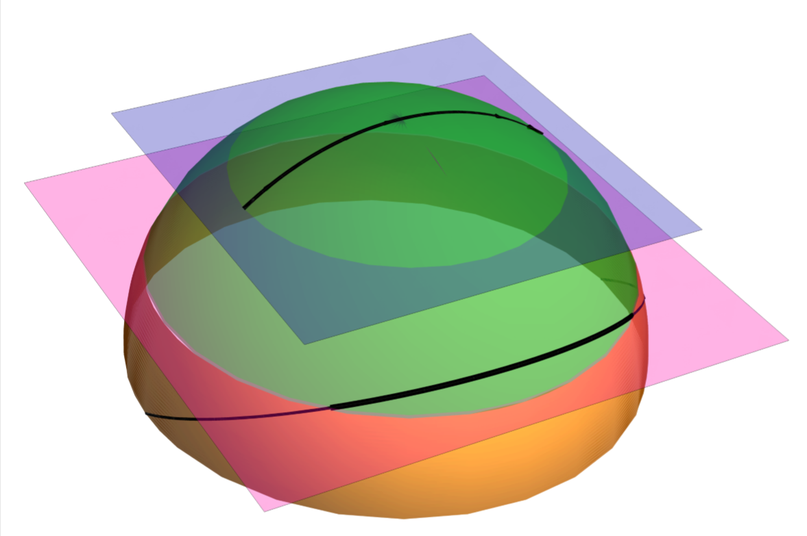
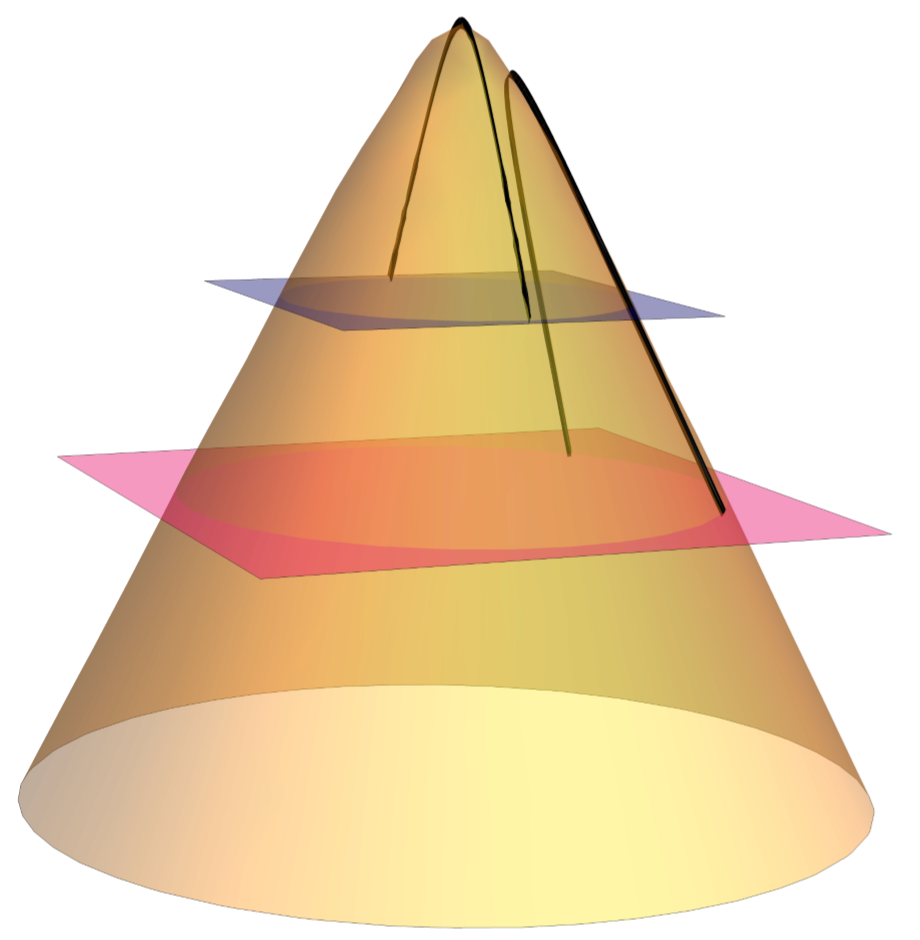
It is important to note that the angle $\beta_{\epsilon}$ measures how much the interval gets smaller compared to an interval of antipodal points on the sphere. The case $\beta_{\epsilon}=0$ corresponds to antipodal points. In order to measure the length of the interval, it makes sense to introduce the angle $\delta=\pi/2-\beta$, with $R_{\text{eff}}=R\cos\theta_{\epsilon}=R\sin\delta$. In order to further confirm our results, we expand the results for pushing the cutoff surface to the boundary. We reach the boundary for $R\to\infty$ (AdS) and $R=L$ (dS), respectively. Introducing the cutoff $\Lambda$, the entanglement entropies for AdS read

	$\displaystyle S^{d=2}_{\text{EE}}(\delta)$	$\displaystyle\!=\!\frac{4\,L\,\pi}{\ell_{p}}\,\left(\log\!\left(\frac{2\,\Lambda\sin(\delta)}{L}\right)+\frac{L^{2}}{4\Lambda^{2}\,\sin(\delta)^{2}}+\mathcal{O}\left(\frac{1}{\Lambda^{3}}\right)\right)$		(21)
	$\displaystyle S^{d=3}_{\text{EE}}(\delta)$	$\displaystyle\!=\!\frac{4\,L\,\pi^{2}}{\ell_{p}^{2}}\!\left(\Lambda\,\sin(\delta)-L+\frac{L^{2}}{2\Lambda\,\sin(\delta)}+\mathcal{O}\left(\frac{1}{\Lambda^{3}}\right)\right)$		(22)
	$\displaystyle S^{d=4}_{\text{EE}}(\delta)$	$\displaystyle\!=\!\frac{4\,\pi^{2}\,L}{\ell_{p}^{3}}\!\left(\Lambda^{2}\sin(\delta)^{2}-\frac{1}{2}L^{2}-L^{2}\log\!\left(\frac{2\,\Lambda\sin(\delta)}{L}\right)+\frac{L^{2}}{4\Lambda^{2}\,\sin(\delta)^{2}}\!+\!\mathcal{O}\!\left(\frac{1}{\Lambda^{2}}\!\right)\!\right)$		(23)
	$\displaystyle S^{d=5}_{\text{EE}}(\delta)$	$\displaystyle\!=\!\frac{4\,\pi^{3}\,L}{3\,\ell_{p}^{4}}\!\left(\Lambda^{3}\,\sin(\delta)^{3}-\frac{3}{2}\Lambda L^{3}\,\sin(\delta)+2L^{3}-\frac{9L^{4}}{8\,\Lambda\,\sin(\delta)}+\mathcal{O}\left(\frac{1}{\Lambda^{3}}\right)\right)$		(24)
	$\displaystyle S^{d=6}_{\text{EE}}(\delta)$	$\displaystyle\!=\!\frac{2\,\pi^{3}\,L^{3}}{3\,\ell_{p}^{5}}\!\left(\!\frac{2\Lambda^{4}\sin(\delta)^{4}}{L^{2}}-2\Lambda^{2}\sin(\delta)^{2}-\!\frac{7\,L^{2}}{4}+3L^{2}\log\!\left(\!\frac{2\Lambda\sin(\delta)}{L}\!\right)\!+\!\mathcal{O}\!\left(\frac{1}{\Lambda^{2}}\!\right)\!\right)\!.$		(25)

which matches the result of Casini, Huerta and Myers Casini:2011kv. The results for $d=2$ match the well known field theory result for a subsystem $\ell$ in a system of length $L$ Holzhey:1994we; Calabrese:2004eu; Calabrese:2005zw

$$S=\frac{c}{3}\,\log\left(\frac{L}{\pi\,a}\,\sin\left(\frac{\pi\ell}{L}\right)\right),$$

(26)

with the cutoff $a$ ($a\to 0$). In the dS case, $\Delta$ in (9) vanishes and we get back the full dS entropy as was observed in Geng:2019bnn.

In general, if we consider entanglement entropies, we expect the result to be divergent, i.e. the leading divergence is the so-called area term Nishioka:2009un; Casini:2003ix; Plenio:2004he; Cramer:2005mx; Das:2005ah. In CFT calculations, however, we usually work with renormalized quantities instead of the bare ones since those quantities are universally well defined and still make sense when we take the continuum limit. The $T\bar{T}$ deformation, on the other hand, acts as UV regulator and all quantities are automatically finite. In principle, we could add an arbitrary amount of counterterms to the dual effective field theory action but we will restrict ourselves to only considering the standard holographic counterterms (deHaro:2000vlm; Skenderis:2002wp). If we add counterterms to the field theory action, living on the cutoff slice, these finite counterterms will affect the result for the entanglement entropy (see for example Murdia:2019fax for a discussion about this) Taylor:2016aoi; Cooperman:2013iqr; Emparan:1999pm; Faulkner:2013ana; Faulkner:2013ica. In the discussion of the next section, we will consider the renormalized stress tensor on the cutoff slice which can be derived by supplementing the gravitational action with counterterms in order to render it finite as explained in deHaro:2000vlm; Skenderis:2002wp. Specifically, we are considering the action

$$S_{\text{tot}}=S_{\text{EH}}+S_{\text{surf}}+S_{\text{ct}},$$

(27)

with

		$\displaystyle S_{\text{EH}}=-\frac{1}{2\,\ell_{p}^{d-1}}\int\mathrm{d}^{d+1}x\,\sqrt{g}\,\left(R^{(d+1)}-2\Lambda\right),$		(28)
		$\displaystyle S_{\text{surf}}=-\frac{1}{\ell_{p}^{d-1}}\int\mathrm{d}^{d}x\,\sqrt{\gamma}\,K,$		(29)
		$\displaystyle S_{\text{ct}}=\frac{1}{2\,\ell_{p}^{d-1}}\int\mathrm{d}^{d}x\,\sqrt{\gamma}\left(\!2\,c_{1}^{(d)}\frac{d-1}{L}+\frac{c^{(d)}_{2}\,L}{d-2}\,\tilde{R}+\frac{c_{3}^{(d)}\,L^{3}}{(d-4)\,(d-2)^{2}}\left(\!\tilde{R}_{ij}\tilde{R}^{ij}-\frac{d}{4\,(d-1)}\tilde{R}^{2}\right)\!\right)\!,$		(30)

where $\tilde{R},\,\tilde{R}_{ab}$ are the Ricci scalar- and tensor, respectively, on the boundary slice with the induced metric $\gamma$. Furthermore, the $c_{i}^{(d)}=1$ in case of: $c_{1}^{(d)}:d\geq 2$, $c_{2}^{(d)}:d\geq 3$ and $c_{3}^{(d)}:d\geq 5$ and $K$ is the extrinsic curvature. In the derivation of the holographic entanglement entropy, we equate the partition function of both theories

$$Z_{\text{CFT,bare}}[\gamma_{ij}]=\left.e^{I_{\text{grav}}[g_{ij}]}\right|_{r=r_{c}}.$$

(31)

However, this is a statement about the bare partition functions of both theories. If we renormalize the field theory partition function, we have to take into account the counterterms in the gravitational theory which act as higher curvature terms on the cutoff slice. Thus, we may take into account the counterterms on the cutoff slice by adding the contributions of the Wald entropy associated with the counterterms to the holographic entanglement entropy. The Wald entropy Wald:1993nt is given by Jacobson:1993vj; Jacobson:1994qe; Brustein:2007jj

$$S_{\text{Wald}}=-2\pi\oint\mathrm{d}^{d}x\,\frac{\delta\mathcal{L}}{\delta\tilde{R}_{abcd}}\,\hat{\epsilon}_{ab}\,\hat{\epsilon}_{cd},$$

(32)

where $\hat{\epsilon}_{ab}$ are the binormals to the horizon. For pedagogical reasons, we rewrite the metric eq. (2) with $R(r)=L\,\sinhh(r/L),R\equiv R(r_{c})$ and $\rho=\cos\phi$

$$\mathrm{d}s^{2}_{\text{DS}}=\mathrm{d}r^{2}+R^{2}(r)\,\left(-(1-\rho^{2})\,\mathrm{d}\tau^{2}+\frac{\mathrm{d}\rho^{2}}{1-\rho^{2}}+\rho^{2}\,\mathrm{d}\Omega_{d-2}\right).$$

(33)

In these coordinates, we see that on the cutoff slice $r/L=r_{c}/L$ in the static patch, the $\hat{\epsilon}_{\tau\rho}$, are the binormals and we have to vary the Lagrangian in eq. (32) with respect to $\tilde{R}_{\tau\rho\tau\rho}$ in order to find the Wald entropy. For the counterterms given in eq. (30), we thus find on the slice $r/L=r_{c}/L$ for an entangling surface with $\rho_{\epsilon}=\cos(\beta_{\epsilon})$ and $R_{\text{eff}}=R(r_{c})\,\rho_{\epsilon}$

	$\displaystyle S_{\text{W,ct}}$	$\displaystyle=-\frac{2\pi}{\ell_{p}^{d-1}}R_{\text{eff}}^{d-2}\,\oint\sqrt{h}\,\left(\frac{c_{2}^{(d)}\,L}{d-2}+\frac{c_{3}^{(d)}L^{3}}{(d-4)(d-2)^{2}}\left(\tilde{R}-h^{ab}\tilde{R}_{ab}-\frac{2d}{4\,(d-1)}\tilde{R}\right)\right)$
		$\displaystyle=-\frac{4\,\pi^{(d+1)/2}\,R_{\text{eff}}^{d-2}}{(d-2)\,\ell_{p}^{d-1}\,\Gamma((d-1)/2)}\left(c_{2}^{(d)}\,L-\frac{c_{3}^{(d)}\,L^{3}}{2\,(d-4)\,R_{\text{eff}}^{2}}\left(d-2\right)\right),$		(34)

where $h_{ab}$ is the induced metric on the unit sphere and where we used that on the cutoff slice $\tilde{R}=d\,(d-1)/R_{\text{eff}}^{2}$ and $R_{ab}=(d-1)/R_{\text{eff}}^{2}\,h_{ab}$. Evaluating the expression in eq. (34) for $3\leq d\leq 6$, we find

	$\displaystyle S^{d=3}_{\text{W,ct}}$	$\displaystyle=-\frac{4\,\pi^{2}\,L\,R_{\text{eff}}}{\ell_{p}^{2}}$		(35)
	$\displaystyle S^{d=4}_{\text{W,ct}}$	$\displaystyle=-\frac{4\,\pi^{2}\,L\,R_{\text{eff}}^{2}}{\ell_{p}^{3}}$		(36)
	$\displaystyle S^{d=5}_{\text{W,ct}}$	$\displaystyle=\frac{\pi^{3}\,L}{\ell_{p}^{3}}\left(-\frac{4\,R_{\text{eff}}^{3}}{5}+2\,R_{\text{eff}}\,L^{2}\right)$		(37)
	$\displaystyle S^{d=6}_{\text{W,ct}}$	$\displaystyle=\frac{\pi^{3}\,L}{\ell_{p}^{4}}\left(-\frac{4\,R_{\text{eff}}^{4}}{3}+\frac{4\,R_{\text{eff}}^{2}\,L^{2}}{3}\right).$		(38)

Note that in $d=2$, we do not see a contribution from the counterterms to the entanglement entropy since the counterterm acts as a boundary cosmological constant.

We may extract the Brown-York stress tensor from the renormalized action eq. (27) by considering

$$\delta S_{\text{tot}}=\frac{1}{2}\int\mathrm{d}^{d}x\,\sqrt{\gamma}\ T^{ij}\,\delta\gamma_{ij},$$

(39)

where $\gamma$ is the induced metric on the cutoff slice. The stress tensor of the boundary field theory $T_{ij}^{\text{bdy}}$ is related to the bulk stress tensor by rescaling $T^{\text{BY}}_{ij}=r_{c}^{d-2}\,T^{\text{bdy}}_{ij}$. This is also true for the metric of the CFT: $g_{ij}(r=r_{c},x)=\gamma_{ij}(x)=r_{c}^{2}\,\gamma_{ij}^{\text{bdy}}(x)$. For a complete dictionary on the cutoff slice see Hartman:2018tkw. In the following discussion, we will set $r_{c}=1$. The holographic stress tensor dual to a $d$-dimensional field theory may be expressed in terms of the extrinsic curvature $K_{ij}$ and the induced quantities on the boundary slice: the metric $\gamma_{ij}$, the Einstein tensor $\tilde{G}_{ij}$, the Riemann tensor $\tilde{R}_{ijkl}$, the Ricci tensor $\tilde{R}_{ij}$ and the Ricci scalar $\tilde{R}$ deHaro:2000vlm; Balasubramanian:1999re; Hartman:2018tkw; Banerjee:2019ewu. The renormalized stress tensor consists of two components $T^{\text{ren}}_{ij}[\gamma]=T_{ij}[\gamma]+C_{ij}[\gamma]$, the standard holographic stress tensor on the cutoff surface $r=r_{c}$, $T_{ij}$, and the corresponding curvature contributions of the counterterms eq. (30), denoted by $C_{ij}$. In order to remove the divergences in the action eq. (27), we add counterterms eq. (30) – which are scalar quantities – to the action. The divergences arise when we push the cutoff surface to the AdS boundary. On the cutoff surface, the stress tensor is automatically regularized and reads

	$\displaystyle T_{ij}=$	$\displaystyle\frac{1}{8\pi G_{N}}\,\left(K_{ij}-K\,\gamma_{ij}-c_{d}^{(1)}\,\frac{d-1}{L}\,\gamma_{ij}+\frac{c_{d}^{(2)}L}{d-2}\,\tilde{G}_{ij}\right.$
		$\displaystyle\left.\ +\frac{c_{d}^{(3)}L^{3}}{(d-4)(d-2)^{2}}\,\left(2\,\left(\tilde{R}_{ijkl}-\frac{1}{4}\,\gamma_{ij}\,\tilde{R}_{kl}\right)\,\tilde{R}^{kl}-\frac{d}{2\,(d-1)}\,\left(\tilde{R}_{ij}-\frac{1}{4}\,\tilde{R}\,\gamma_{ij}\right)\tilde{R}\right.\right.$
		$\displaystyle\ \left.\left.-\frac{1}{2\,(d-1)}\left(\gamma_{ij}\,\Box\tilde{R}+(d-2)\,\nabla_{i}\,\nabla_{j}\tilde{R}\right)+\Box\tilde{R}_{ij}\right)\right),$		(40)

with $\ell_{P}^{d-1}=8\pi\,G_{N}$. With eq. (30) and eq. (39) the curvature dependent counterterms give thus rise to the contribution (in $d\geq 3$) deHaro:2000vlm; Skenderis:2002wp

	$\displaystyle C_{ij}=$	$\displaystyle-\frac{1}{8\pi G_{N}}\,\left(c_{d}^{(2)}\,\tilde{G}_{ij}+c_{d}^{(3)}\,b_{d}\,\left[2\left(\tilde{R}_{ikjl}-\frac{1}{4}\,\gamma_{ij}\,\tilde{R}_{kl}\right)\,\tilde{R}^{kl}-\frac{d}{2(d-1)}\,\left(\tilde{R}_{ij}-\frac{1}{4}\,\tilde{R}\,\gamma_{ij}\right)\tilde{R}\right.\right.$
		$\displaystyle\left.\left.-\frac{1}{2\,(d-1)}\left(\gamma_{ij}\,\Box\tilde{R}+(d-2)\,\nabla_{i}\nabla_{j}\tilde{R}\right)+\Box\tilde{R}_{ij}\right]\right),$		(41)

with $b_{d}=l^{2}/((d-4)(d-2))$. The $c^{(d)}_{i}$’s are non-zero in case of: $c^{(d)}_{2}=1$ for $d\geq 3$ and $c^{(d)}_{3}=1$ for $d\geq 5$. Deforming a theory by a local operator $X$ results, on the level of the classical action, in

$$\frac{\partial S}{\partial\lambda}=\int d^{d}x\,\sqrt{\gamma}X,$$

(42)

with $\lambda$ being the size of the deformation. In $d=2$, the $T\bar{T}$ deformation satisfies the factorization property Zamolodchikov:2004ce

$$\langle T\bar{T}\rangle=\frac{1}{8}\,\left(\langle T^{ij}\rangle\langle T_{ij}\rangle-\langle T_{i}^{i}\rangle^{2}\right).$$

(43)

In general, this would no longer be true in higher dimensions. However, since we are working in a CFT at large $N$, the factorization property is still valid at $d>2$ McGough:2016lol; Hartman:2018tkw.

In order to derive the deforming operator $X_{d}=-\frac{1}{d\,\lambda_{d}}T^{i}_{i}$, we derive the trace flow equation for the holographic stress tensor using Einstein’s equations. This is accomplished by using the general form of the holographic stress tensor (40) and then by using the Hamilton constraint in appendix A. The d-dimensional expression is given by

$\displaystyle X_{d}=\!\left(T_{ij}\!+\!\frac{\alpha_{d}}{\lambda_{d}^{\frac{d-2}{d}}}C_{ij}\!\right)^{\!2}\!\!\!-\!\frac{1}{d-1}\left(T^{i}_{i}\!+\!\frac{\alpha_{d}}{\lambda_{d}^{\frac{d-2}{d}}}C_{i}^{i}\!\right)^{\!2}\!\!+\!\frac{1}{d}\frac{\alpha_{d}}{\lambda_{d}^{\frac{2(d-1)}{d}}}\!\left(\frac{d-2}{2}\mathcal{R}^{(d)}\!+\!C^{i}_{i}\!\right)\!+\!\frac{(d-1)(\eta-1)}{4\,d\,\lambda_{d}^{2}},$

(44)

where $\eta=1$ corresponds to the AdS case and $\eta=-1$ to the dS case, respectively. Furthermore, the $\alpha_{d}$ are dimensionless numbers and correspond to the number of degrees of freedom in the field theory. We denote the coupling of the deformations by $\lambda_{d}$. The parameters of the field theory are related to the parameters on the gravity side by Banerjee:2019ewu

$$\lambda_{d}=\frac{\ell_{P}^{d-1}\,L}{2d},\quad\alpha_{d}=\frac{L^{2(d-1)/d}}{(2d)^{\frac{d-2}{d}}\,(d-2)\,\ell_{P}^{\frac{2\,(d-1)}{d}}},\quad L^{2}=2d\,(d-2)\,\alpha_{d}\,\lambda^{2/d}_{d}.$$

(45)

In a two-dimensional CFT, the central charge $c$ is related to the bulk quantities as Brown:1986nw

$$c=\frac{12\pi L}{\ell_{P}}.$$

(46)

For example in $d=2$ dimensions the deforming operator reads

$$X_{2}=T_{ij}^{2}-\frac{1}{d-1}(T^{i}_{i})^{2}+\frac{1}{2\lambda}\,\frac{c}{24\pi}\,R+\frac{\eta-1}{8\lambda^{2}},$$

(47)

which matches the result of Gorbenko:2018oov.

Let us consider a generic seed CFT in $d$-dimensions at large central charge on a sphere with radius $R$. Our goal is to compute the exact sphere partition function $Z_{S^{d}}$. From the sphere partition function, it is straightforward to calculate the entanglement entropy for antipodal points on the sphere as was outlined by Donnelly:2018bef. What we are interested in is the change of the partition function in response to deformations of the sphere. As argued in Donnelly:2018bef; Banerjee:2019ewu and since changes of the metric manifest in the vacuum expectation value of the stress tensor, the symmetries on the sphere dictate

$$\langle T_{ij}\rangle=\omega_{d}(R)\,\gamma_{ij}$$

(48)

we can write the deformation of the $d-$dimensional sphere partition function as

$$R\frac{\partial}{\partial R}\,\log Z_{S^{d}}=-d\,\int d^{d}x\,\sqrt{\gamma}\,\omega_{d}(R),$$

(49)

from which we can compute the entanglement entropy using the replica trick. It now becomes apparent why we chose dS slicing for (A)dS in the first place: the dS ground state corresponds to the Euclidean path integral on the sphere $S^{d}$.

We may apply the replica trick by considering the $n$-folded cover of the sphere of radius $R$ Donnelly:2018bef; Banerjee:2019ewu

$$ds^{2}=R^{2}\left(d\theta_{1}^{2}+\sum_{i=2}^{d-1}\prod_{j=1}^{i-1}\cos(\theta_{j})^{2}\,d\theta_{i}^{2}+n^{2}\,\prod_{j=1}^{d-1}\cos(\theta_{j})^{2}\,d\theta_{d}^{2}\right),$$

(50)

with $\theta_{j}\in[-\pi/2,\pi/2]$ for $j=1,\ldots,d-1$ and $\theta_{d}\in[0,2\pi]$. For simplicity, we set $d=2$ for now which reduces (50) to

$$ds^{2}=R^{2}\,(d\theta^{2}+n^{2}\cos(\theta)^{2}d\phi^{2}),$$

(51)

with $\phi\in[0,2\pi]$ and $\theta\in[-\pi/2,\pi/2]$. The angle $\theta$ is chosen so that it corresponds to the angle $\theta$ in the gravitational theory; it is the azimuthal angle on the sphere and the antipodal points $\theta=-\pi/2$ and $\theta=\pi/2$ correspond to the north and south pole of the sphere. Since the entangling surface consists of two antipodal points we may – due to the rotational symmetry – continuously vary $n$ which allows us to compute the entanglement entropy with

$$S_{\text{d,EE}}=\left(1-\frac{R}{d}\frac{d}{dR}\right)\log Z_{S^{d}}.$$

(52)

In order to calculate the sphere partition function (49), we compute the expression for $\omega_{d}$ using the flow equation $\langle T^{i}_{i}\rangle=-d\,\lambda_{d}\,\langle X_{d}\rangle$. With help of the deforming operator $X_{d}$ (defined in eq. (44)), we end up with a quadratic equation for $\omega_{d}$. To derive an explicit expression for $\omega_{d}$, we have to evaluate the stress energy tensor and the counterterms for a $d$-dimensional sphere of radius $R$. The quadratic equation yields a positive and a negative solution so there are two possible signs for the $T\bar{T}$ deformation. For now, we will denote the signs of the square root simply by $\bm{s}$. In the case $d=2$ all the $c^{\prime}s$ are zero and it is straightforward to check that

$$\omega_{2}=\frac{1+\bm{s}\sqrt{\eta+\frac{c\,\lambda_{2}}{3\pi\,R^{2}}}}{4\,\lambda_{2}}.$$

(53)

Since we are working in a large $N$ CFT where the coupling of the deformation $\lambda^{2/d}$ is small but $N\lambda^{2/d}$ is finite, we may write (in $d>2$) the expansion parameter as $t_{d}=\alpha_{d}\lambda^{2/d}$. With this, we find the expression for the sphere partition function in $d>2$ to be

	$\displaystyle\omega_{d>2}=$	$\displaystyle\frac{(-1+d)}{4\,d\,R^{4}\,\lambda_{d}}\left(\!2\,(d-2)\,d\,R^{2}\,\lambda^{2/d}\,c_{d}^{(2)}\,\alpha_{d}-(d-2)^{2}\,d^{2}\,\lambda^{4/d}\,c_{d}^{(3)}\,\alpha_{d}^{2}\right.$
		$\displaystyle\left.+2R^{3}\,\left(R+\bm{s}\,\sqrt{\eta\,R^{2}+2\,(d-2)\,d\,\lambda^{2/d}\alpha_{d}}\right)\right)$		(54)

From the expression for $\omega_{d}$, it is straightforward to calculate the entanglement entropy. The procedure goes as follows: we are taking $\omega$ from eq. (53) and (54), respectively and inserting them into eq. (49); this yields an expression for the $R$-derivative of the partition function. To obtain the entanglement entropy, we must first integrate the expression and plug the result into eq. (52). However, this integration results in an integration constant that must be fixed before proceeding. We may fix the integration constant either in the IR or the UV region of the theory. In $d=2$, we may follow Gorbenko:2018oov and fix the integration constant by matching the partition function for AdS in the $R^{2}/\lambda_{2}\to\infty$ limit to the CFT partition function

$$\log Z_{\text{CFT}}(R)=\frac{c}{3}\,\log\frac{R}{a}.$$

(55)

The integration constant for the dS case is obtained by matching the partition function in the $R^{2}/\lambda\to 0$ case to the AdS partition function⁵⁵ 5 Note that $a$ is an arbitrary cutoff scale and not determined by the CFT itself. The value of the UV scale may be adjusted later. This implies that we have not fixed the integration constant before fixing the UV scale. However, if we consider cutoff independent quantities as $\mathcal{S}_{\text{R,EE}}$ this constant does not contribute.. However, the CFT partition function is not known in $d>2$ and we chose to follow Donnelly:2018bef, which fixes the integration constant by demanding the logarithm of the partition function to vanish for $R^{2}/\lambda\to 0$. This leads to a trivial theory in the UV. Note that this is only possible in presence of the UV cutoff since the theory does not change as a function of the scale at arbitrarily short distances anymore.

There is a different way to extract the universal quantities of the entanglement entropy as the approach we took in section 2.4 based on Taylor:2016aoi; Cooperman:2013iqr. In analogy to Gorbenko:2018oov; Banerjee:2019ewu; Liu:2012eea; Liu:2013una, we also compute the cutoff independent renormalized entanglement entropy⁶⁶ 6 In contrast to Banerjee:2019ewu, we follow the convention of Liu:2012eea; Liu:2013una with the double factorial.

$$\mathcal{S}_{\text{R,EE}}(R)=\begin{cases}\frac{R}{(d-2)!!}\,R\,\frac{d}{dR}(R\,\frac{d}{dR}-2)\ldots(R\,\frac{d}{dR}-(d-2))\,S_{\text{EE}}\quad\quad\quad\quad\text{d even},\\ \frac{R}{(d-2)!!}(R\,\frac{d}{dR}-1)(R\,\frac{d}{dR}-3)\ldots(R\,\frac{d}{dR}-(d-2))\,S_{\text{EE}}\quad\quad\text{d odd.}\end{cases}$$

(56)

References

- (1) F. A. Smirnov and A. B. Zamolodchikov, On space of integrable quantum field theories, Nucl. Phys. B915 (2017) 363–383, 1608.05499.
- (2) A. Cavaglià, S. Negro, I. M. Szécsényi, and R. Tateo, -deformed 2D Quantum Field Theories, JHEP 10 (2016) 112, 1608.05534.
- (3) A. B. Zamolodchikov, Expectation value of composite field T anti-T in two-dimensional quantum field theory, hep-th/0401146.
- (4) L. McGough, M. Mezei, and H. Verlinde, Moving the CFT into the bulk with , JHEP 04 (2018) 010, 1611.03470.
- (5) S. Dubovsky, V. Gorbenko, and M. Mirbabayi, Asymptotic fragility, near AdS2 holography and , JHEP 09 (2017) 136, 1706.06604.
- (6) H.-S. Jeong, K.-Y. Kim, and M. Nishida, Entanglement and Rényi Entropy of Multiple Intervals in -Deformed CFT and Holography, 1906.03894.
- (7) J. Cardy, The deformation of quantum field theory as random geometry, JHEP 10 (2018) 186, 1801.06895.
- (8) L. Apolo and W. Song, Heating up holography for single-trace deformations, 1907.03745.
- (9) W. Cottrell and A. Hashimoto, Comments on double trace deformations and boundary conditions, Phys. Lett. B789 (2019) 251–255, 1801.09708.
- (10) M. Guica and R. Monten, and the mirage of a bulk cutoff, 1906.11251.
- (11) P. Kraus, J. Liu, and D. Marolf, Cutoff AdS3 versus the deformation, JHEP 07 (2018) 027, 1801.02714.
- (12) W. Donnelly and V. Shyam, Entanglement entropy and deformation, Phys. Rev. Lett. 121 (2018), no. 13 131602, 1806.07444.
- (13) T. Hartman, J. Kruthoff, E. Shaghoulian, and A. Tajdini, Holography at finite cutoff with a deformation, JHEP 03 (2019) 004, 1807.11401.
- (14) M. Taylor, TT deformations in general dimensions, 1805.10287.
- (15) G. Bonelli, N. Doroud, and M. Zhu, -deformations in closed form, JHEP 06 (2018) 149, 1804.10967.
- (16) B. Le Floch and M. Mezei, Solving a family of -like theories, 1903.07606.
- (17) O. Aharony and T. Vaknin, The TT* deformation at large central charge, JHEP 05 (2018) 166, 1803.00100.
- (18) S. Chakraborty, A. Giveon, and D. Kutasov, , , and String Theory, 1905.00051.
- (19) D. J. Gross, J. Kruthoff, A. Rolph, and E. Shaghoulian, in AdS2 and Quantum Mechanics, 1907.04873.
- (20) O. Aharony, S. Datta, A. Giveon, Y. Jiang, and D. Kutasov, Modular invariance and uniqueness of deformed CFT, JHEP 01 (2019) 086, 1808.02492.
- (21) S. Datta and Y. Jiang, deformed partition functions, JHEP 08 (2018) 106, 1806.07426.
- (22) A. Giveon, N. Itzhaki, and D. Kutasov, and LST, JHEP 07 (2017) 122, 1701.05576.
- (23) V. Shyam, Background independent holographic dual to deformed CFT with large central charge in 2 dimensions, JHEP 10 (2017) 108, 1707.08118.
- (24) C. Murdia, Y. Nomura, P. Rath, and N. Salzetta, Comments on holographic entanglement entropy in deformed conformal field theories, Phys. Rev. D100 (2019), no. 2 026011, 1904.04408.
- (25) V. Shyam, Finite Cutoff AdS5 Holography and the Generalized Gradient Flow, JHEP 12 (2018) 086, 1808.07760.
- (26) Y. Jiang, Expectation value of operator in curved spacetimes, 1903.07561.
- (27) C. Park, Holographic Entanglement Entropy in Cutoff AdS, Int. J. Mod. Phys. A33 (2019), no. 36 1850226, 1812.00545.
- (28) M. Guica, An integrable Lorentz-breaking deformation of two-dimensional CFTs, SciPost Phys. 5 (2018), no. 5 048, 1710.08415.
- (29) M. Baggio, A. Sfondrini, G. Tartaglino-Mazzucchelli, and H. Walsh, On deformations and supersymmetry, JHEP 06 (2019) 063, 1811.00533.
- (30) C.-K. Chang, C. Ferko, and S. Sethi, Supersymmetry and deformations, JHEP 04 (2019) 131, 1811.01895.
- (31) B. Chen, L. Chen, and C.-Y. Zhang, Surface/State correspondence and deformation, 1907.12110.
- (32) T. Ota, Comments on holographic entanglements in cutoff AdS, 1904.06930.
- (33) J. Cardy, deformation of correlation functions, 1907.03394.
- (34) A. Banerjee, A. Bhattacharyya, and S. Chakraborty, Entanglement Entropy for deformed CFT in general dimensions, 1904.00716.
- (35) P. Caputa, S. Datta, and V. Shyam, Sphere partition functions and cut-off AdS, 1902.10893.
- (36) V. Gorbenko, E. Silverstein, and G. Torroba, dS/dS and , 1811.07965.
- (37) A. Sfondrini and S. J. van Tongeren, deformations as TsT transformations, 1908.09299.
- (38) S. Chakraborty, A. Giveon, N. Itzhaki, and D. Kutasov, Entanglement beyond AdS, Nucl. Phys. B935 (2018) 290–309, 1805.06286.
- (39) Y. Jiang, Lectures on solvable irrelevant deformations of 2d quantum field theory, 1904.13376.
- (40) P. Calabrese and J. L. Cardy, Entanglement entropy and quantum field theory, J. Stat. Mech. 0406 (2004) P06002, hep-th/0405152.
- (41) S. Ryu and T. Takayanagi, Holographic derivation of entanglement entropy from AdS/CFT, Phys. Rev. Lett. 96 (2006) 181602, hep-th/0603001.
- (42) B. Chen, L. Chen, and P.-X. Hao, Entanglement entropy in -deformed CFT, Phys. Rev. D98 (2018), no. 8 086025, 1807.08293.
- (43) M. Alishahiha, A. Karch, E. Silverstein, and D. Tong, The dS/dS correspondence, AIP Conf. Proc. 743 (2005) 393–409, hep-th/0407125, [,393(2004)].
- (44) M. Alishahiha, A. Karch, and E. Silverstein, Hologravity, JHEP 06 (2005) 028, hep-th/0504056.
- (45) X. Dong, B. Horn, E. Silverstein, and G. Torroba, Micromanaging de Sitter holography, Class. Quant. Grav. 27 (2010) 245020, 1005.5403.
- (46) B. Freivogel, Y. Sekino, L. Susskind, and C.-P. Yeh, A Holographic framework for eternal inflation, Phys. Rev. D74 (2006) 086003, hep-th/0606204.
- (47) X. Dong, B. Horn, S. Matsuura, E. Silverstein, and G. Torroba, FRW solutions and holography from uplifted AdS/CFT, Phys. Rev. D85 (2012) 104035, 1108.5732.
- (48) A. Karch, Autolocalization in de Sitter space, JHEP 07 (2003) 050, hep-th/0305192.
- (49) X. Dong, E. Silverstein, and G. Torroba, De Sitter Holography and Entanglement Entropy, JHEP 07 (2018) 050, 1804.08623.
- (50) H. Geng, S. Grieninger, and A. Karch, Entropy, Entanglement and Swampland Bounds in DS/dS, JHEP 06 (2019) 105, 1904.02170.
- (51) H. Casini, M. Huerta, and R. C. Myers, Towards a derivation of holographic entanglement entropy, JHEP 05 (2011) 036, 1102.0440.
- (52) C. Holzhey, F. Larsen, and F. Wilczek, Geometric and renormalized entropy in conformal field theory, Nucl. Phys. B424 (1994) 443–467, hep-th/9403108.
- (53) P. Calabrese and J. L. Cardy, Entanglement entropy and quantum field theory: A Non-technical introduction, Int. J. Quant. Inf. 4 (2006) 429, quant-ph/0505193.
- (54) T. Nishioka, S. Ryu, and T. Takayanagi, Holographic Entanglement Entropy: An Overview, J. Phys. A42 (2009) 504008, 0905.0932.
- (55) H. Casini, Geometric entropy, area, and strong subadditivity, Class. Quant. Grav. 21 (2004) 2351–2378, hep-th/0312238.
- (56) M. B. Plenio, J. Eisert, J. Dreissig, and M. Cramer, Entropy, entanglement, and area: analytical results for harmonic lattice systems, Phys. Rev. Lett. 94 (2005) 060503, quant-ph/0405142.
- (57) M. Cramer, J. Eisert, M. B. Plenio, and J. Dreissig, An Entanglement-area law for general bosonic harmonic lattice systems, Phys. Rev. A73 (2006) 012309, quant-ph/0505092.
- (58) S. Das and S. Shankaranarayanan, How robust is the entanglement entropy: Area relation?, Phys. Rev. D73 (2006) 121701, gr-qc/0511066.
- (59) S. de Haro, S. N. Solodukhin, and K. Skenderis, Holographic reconstruction of space-time and renormalization in the AdS / CFT correspondence, Commun. Math. Phys. 217 (2001) 595–622, hep-th/0002230.
- (60) K. Skenderis, Lecture notes on holographic renormalization, Class. Quant. Grav. 19 (2002) 5849–5876, hep-th/0209067.
- (61) M. Taylor and W. Woodhead, Renormalized entanglement entropy, JHEP 08 (2016) 165, 1604.06808.
- (62) J. H. Cooperman and M. A. Luty, Renormalization of Entanglement Entropy and the Gravitational Effective Action, JHEP 12 (2014) 045, 1302.1878.
- (63) R. Emparan, C. V. Johnson, and R. C. Myers, Surface terms as counterterms in the AdS / CFT correspondence, Phys. Rev. D60 (1999) 104001, hep-th/9903238.
- (64) T. Faulkner, A. Lewkowycz, and J. Maldacena, Quantum corrections to holographic entanglement entropy, JHEP 11 (2013) 074, 1307.2892.
- (65) T. Faulkner, M. Guica, T. Hartman, R. C. Myers, and M. Van Raamsdonk, Gravitation from Entanglement in Holographic CFTs, JHEP 03 (2014) 051, 1312.7856.
- (66) R. M. Wald, Black hole entropy is the Noether charge, Phys. Rev. D48 (1993), no. 8 R3427–R3431, gr-qc/9307038.
- (67) T. Jacobson, G. Kang, and R. C. Myers, On black hole entropy, Phys. Rev. D49 (1994) 6587–6598, gr-qc/9312023.
- (68) T. Jacobson, G. Kang, and R. C. Myers, Black hole entropy in higher curvature gravity, in Heat Kernels and Quantum Gravity Winnipeg, Canada, August 2-6, 1994, 1994. gr-qc/9502009.
- (69) R. Brustein, D. Gorbonos, and M. Hadad, Wald’s entropy is equal to a quarter of the horizon area in units of the effective gravitational coupling, Phys. Rev. D79 (2009) 044025, 0712.3206.
- (70) V. Balasubramanian and P. Kraus, A Stress tensor for Anti-de Sitter gravity, Commun. Math. Phys. 208 (1999) 413–428, hep-th/9902121.
- (71) J. D. Brown and M. Henneaux, Central Charges in the Canonical Realization of Asymptotic Symmetries: An Example from Three-Dimensional Gravity, Commun. Math. Phys. 104 (1986) 207–226.
- (72) H. Liu and M. Mezei, A Refinement of entanglement entropy and the number of degrees of freedom, JHEP 04 (2013) 162, 1202.2070.
- (73) H. Liu and M. Mezei, Probing renormalization group flows using entanglement entropy, JHEP 01 (2014) 098, 1309.6935.