Constraining Nonthermal Dark Matter’s Impact on the Matter Power Spectrum

In the above system of equations, we do not allow for scattering interactions between the dark matter and SM particles. Also, we neglect both the thermal production and self-annihilation of dark matter particles, effectively assuming that the velocity-averaged annihilation cross section is small enough that any amount of dark matter lost to annihilations is negligible and any produced thermally is negligible compared to that produced from scalar decay. However, if dark matter annihilations are $s$-wave, neglecting annihilations does not change the results of our conclusions because we are interested in the average dark matter velocity and the fraction of dark matter that has lost sufficient momentum to participate in structure formation. These quantities are dependent on the velocity distribution of dark matter. For $s$-wave annihilations, the velocity-averaged cross section is independent of particle velocity, and the distribution of particle velocities would be unaffected by the inclusion of annihilations.

Without annihilations, constraining the reheat temperature to be above 3 MeV, as required by BBN, leads to a direct constraint on the fraction of the scalar’s energy imparted to the dark matter: $f\lesssim 10^{-7}$ Erickcek and Sigurdson 2011 for nonrelativistic dark matter. This branching ratio is quite small and it would be more natural to expect the energy imparted in the decay of the scalar to be more evenly allocated to both the dark matter and the SM. The inclusion of annihilations, however, significantly reduces the ratio of dark matter to radiation. This can allow for a more balanced transfer of energy, $f\sim 0.5$, while still achieving a sufficiently small dark matter abundance through annihilations Fan et al. 2014; Gelmini et al. 2006. For relativistic dark matter, its abundance is also dependent on the velocity imparted to the particles at decay $(v_{D})$.

In our model, we consider the scenario in which the dark matter is produced via a two-body decay so that all dark matter particles are born with the same velocity, $v_{D}$. The energy density and decay rate of the scalar then govern the evolution of the equation of state $w_{\chi}$ for the dark matter particles during the EMDE. The rates at which new particles are produced and the momentum of existing particles redshifts away determine the average energy per particle of the dark matter:

where $\hat{n}_{\chi}$ is the comoving number density of the dark matter particles, $v(a,a_{D})$ is the velocity at $a$ of a dark matter particle created at $a_{D}$, and we integrate over $a_{D}$ with $a=1$ setting the onset of dark matter production.

When evaluating Eq. (3) we use the fact that the comoving number density of the dark matter evolves according to

where $\hat{n}_{\phi}$ is the comoving number density of $\phi$ particles, and $b$ is the number of dark matter particles produced per scalar decay. We can then (following a procedure similar to that in Ref. Blackadder and Koushiappas 2014) express the term $d\hat{n}_{\chi}/da_{D}$ as

The constants $b$, $\Gamma_{\phi}$, and $m_{\phi}$ appear in both integrals in Eq. (3) and consequently do not affect $\langle E\rangle$. We numerically evaluate Eq. (3) to obtain the average energy as a function of the scale factor; this is made even simpler by noting that the contribution of the dark matter to the expansion rate at the time of decay, $H_{D}$, is entirely negligible compared to both the scalar and radiation energy densities. The calculation of the average energy then informs how the dark matter equation of state evolves:

The mass of the dark matter particle can be pulled from both the average energy and its derivative, and so $w_{\chi}$ at any given time depends only on the average velocity.

Using Eq. (6), we numerically solve the set of equations in Eq. (2) with the initial condition $a_{i}\equiv a(t_{i})=1$, and we assume there is no dark matter in existence prior to this time. Figure 1 shows the evolution of the scalar, radiation, and relativistic $(v_{D}=0.99)$ and nonrelativistic $(v_{D}=0.1)$ dark matter energy densities in our model. The energy densities in the figure are given as fractions of the initial critical energy density $\rho_{\mathrm{crit},i}$.

In Fig. 1, we have chosen to fix $f=10^{-7}$, which directly sets the relative abundance of dark matter to radiation during the EMDE to be $\sim\!\!10^{-7}$, and we have chosen a scalar decay rate $\tilde{\Gamma}_{\phi}\equiv\Gamma_{\phi}/H_{i}=10^{-10}$, which sets $a_{\mathrm{RH}}\equiv\tilde{\Gamma}^{-2/3}\simeq 5\times 10^{6}$. It is worth noting that, by this definition, $a_{\mathrm{RH}}\neq a|_{T=T_{\mathrm{RH}}}$. The numerical solutions to Eq. (2) show that by a scale factor of $3a_{\mathrm{RH}}$ enough of the scalar has decayed away that it is a negligible source of radiation. As a result, the radiation energy density then evolves as in the usual radiation-dominated era from a temperature $T(3a_{\mathrm{RH}})\simeq 0.34T_{\mathrm{RH}}$ onward. This sets the relation between $a_{\mathrm{RH}}$ and $T_{\mathrm{RH}}$ to be $a_{\mathrm{RH}}/a_{0}=1.54(T_{0}/T_{\mathrm{RH}})g_{*S}^{-1/3}(0.34T_{\mathrm{RH}})$, where $g_{*S}$ is the number of relativistic degrees of freedom in the entropy density.

The effects of the dark matter particles’ velocities can already been seen in Fig. 1. During the EMDE, the energy density of any species, relativistic or nonrelativistic, sourced by scalar decay evolves as $\rho\propto a^{-3/2}$. At the end of the EMDE, when the scalar field is no longer sourcing new particles, the energy densities of the decay products will begin to scale as $\rho\propto a^{-3(w+1)}$. For a scenario in which dark matter is born relativistic, the average value of $w_{\chi}$ during reheating is close to $1/3$, and the dark matter behaves more like radiation. In Fig. 1 we can see that, following reheating, the energy density of relativistic dark matter (dotted) redshifts away faster than its nonrelativistic counterpart (dashed). Once the scalar field has decayed completely and there is no creation of new, hot particles, the existing particles’ momenta continue to redshift until the average particle is no longer relativistic, and after that, the dark matter density scales as $a^{-3}$.

Increasing the velocity imparted to the dark matter particles upon their creation increases the time it takes after reheating for the dark matter energy density to begin scaling as $a^{-3}$, thus increasing the duration of radiation domination for a given value of $f$. The temperature at matter-radiation equality is $T_{\mathrm{eq}}=0.796\pm 0.005$ eV Aghanim et al. 2018, and so a longer radiation-dominated era implies a higher temperature at reheating. For a fixed value of $f$, the reheat temperature that matches the observed dark matter abundance in a scenario of relativistically produced dark matter is a factor of $\gamma_{D}$ greater than that of nonrelativistic dark matter, where $\gamma_{D}$ is the Lorentz factor of the relativistic dark matter particle at production. For a given reheat temperature, the value of $f$ required to produce the observed dark matter abundance is

In the absence of annihilations, the dark matter density during the EMDE is also determined by $f$: if $v_{D}\ll 1$ then $\rho_{\chi}/\rho_{r}\simeq(5/3)f$ Erickcek and Sigurdson 2011, whereas if $v_{D}\simeq 1$ then $\rho_{\chi}/\rho_{r}\simeq f$. In the latter case, $\rho_{\chi}/\rho_{r}\simeq f$ continues until the dark matter is no longer relativistic or changes in $g_{*}$ disrupt the $a^{-4}$ scaling of $\rho_{r}$. Therefore, for $\gamma_{D}\gg 1$, obtaining the observed dark matter abundance requires that $\rho_{\chi}/\rho_{r}\simeq 2.3\times 10^{-7}(3\mathrm{MeV}/T_{\mathrm{RH}})\gamma_{D}$ shortly after reheating. This requirement applies regardless of whether or not annihilations alter the dark matter abundance during the EMDE. After reheating, but while the dark matter is still relativistic, the relative dark matter abundance will evolve as

in either case.

If dark matter is still relativistic at neutrino decoupling, it could affect the predictions of BBN. Dark matter produced relativistically at reheating would still be relativistic ($\gamma\gtrsim 2$) when $T=10$ MeV if

Relativistic dark matter behaves as an additional radiation component, and can be characterized as a change in the number of effective neutrinos, $\Delta N_{\mathrm{eff}}$. The energy density in relativistic particles can be written as

where $T_{\nu}$ is the neutrino temperature, which we assume evolves as $a^{-1}$ after $T=T_{\nu}=10$ MeV, when $g_{*}=g_{*S}=10.75$. Thus, the fractional component of the energy density in dark matter at 10 MeV is related to $\Delta N_{\mathrm{eff}}$ by

Bounds from BBN constrain $N_{\mathrm{eff}}=2.88\pm 0.54$ at 95% C.L. Pitrou et al. 2018, yielding an upper bound $f_{10\mathrm{MeV}}<0.028$. If the dark matter is still relativistic at BBN, then achieving the observed relic abundance requires $f_{10\mathrm{MeV}}\simeq 5\times 10^{-7}\gamma_{D}(3\mathrm{MeV}/T_{\mathrm{RH}})g_{*S}^{-1/3}(0.34T_{\mathrm{RH}})$, as given by Eq. (8). Therefore, the upper bound on $f_{10\mathrm{MeV}}$ translates to a bound on $\gamma_{D}$: $\gamma_{D}\lesssim 5.4\times 10^{4}(T_{\mathrm{RH}}/3\mathrm{MeV})g_{*S}^{1/3}(0.34T_{\mathrm{RH}})$.

This upper bound on $\gamma_{D}$ implies an upper bound on the value of $f$ in Eq. (7) that can result in the observed relic abundance We will see in Section IV that restrictions from small-scale structure on the parameter space of $\gamma_{D}$ and $T_{\mathrm{RH}}$ provide much stronger bounds. As such, annihilations are still necessary to reduce the dark matter abundance to its required value following reheating without fine-tuning $f$.

Given that the momentum of a particle scales as $p\propto a^{-1}$, a particle born from a decay at a scale factor $a_{D}$, with a physical velocity $v_{D}$, has a velocity at some later time given by

The average velocity over all the dark matter particles at any given time is then

which can be evaluated in the same manner as Eq. (3).

Figure 2 shows the evolution of the average dark matter particle velocity throughout the EMDE until just after reheating; the various curves in Fig. 2 represent different values of $v_{D}$. We can see that the average velocity is initially dominated by the few particles born immediately with the imparted velocity. The velocity of these particles begins to redshift away, pulling the average down, until a steady state is reached between the redshifting of the velocity of existing particles and the creation of new, hot particles.

In the regime where the average velocity has reached a constant value - deep into the EMDE and well before reheating - we can simplify our calculation of the average velocity even further and analytically solve the integrals of Eq. (13). During the EMDE, the energy density of the Universe is dominated by the scalar field, and our expression in Eq. (5) becomes

Rewriting the expression for $v^{2}$ to make its dependence on the integration variable, $a_{D}$, more apparent, we have

where $X\equiv\gamma_{D}v_{D}$. And so, deep in the EMDE, our expression for the average velocity, given by Eq. (13), takes the form

The solution to the integral in the numerator is given by

The solution to the integral in the denominator is simply

Long after the decays have started ($a\gg 1$), both integrals scale as $a^{3/2}$ and $\langle v^{2}(a)\rangle$ is constant until just prior to reheating, at which point our approximation in Eq. (14) is no longer valid.

The steady state between the cooling of old particles and the creation of new, hot ones is maintained until just before reheating, and the average dark matter velocity at reheating is not reduced significantly from the velocity imparted at the scalar’s decay. Relativistic-born dark matter, $v_{D}=0.99$, is still considerably relativistic at reheating, $\sqrt{\langle v^{2}\rangle}\simeq 0.93$. At reheating, the average dark matter particle is nonrelativistic only if $v_{D}$ is already largely nonrelativistic: $\sqrt{\langle v^{2}\rangle}\lesssim 0.01$ requires $v_{D}<0.017$.

If the comoving size of the horizon at reheating, $k_{\mathrm{RH}}^{-1}=(a_{\mathrm{RH}}H_{\mathrm{RH}})^{-1}$, is smaller than the dark matter free-streaming horizon, $k_{\mathrm{fs}}^{-1}$, then the random drift of dark matter particles will erase the growth of density perturbations that occurred during the EMDE. Reference Erickcek and Sigurdson 2011 found that $k_{\mathrm{RH}}/k_{\mathrm{fs}}<1$ required the dark matter velocity at reheating to be $v_{\mathrm{RH}}\lesssim 0.06$. Preserving enhanced structure growth requires an even smaller average velocity. Achieving such a small average velocity at reheating would require the dark matter particles to be born with a similarly small velocity.

We begin by calculating the physical streaming length today of a particle born at reheating:

The choice of $a_{D}=a_{\mathrm{RH}}$ is beneficial in that the fraction of dark matter born before reheating, found by our previous analysis of the distribution of birth times, is $0.51$, and we can say that approximately half of the dark matter will have a free-streaming length above or below our calculated value. Another benefit of this choice is that our calculations of the free-streaming length are made simpler by neglecting the contribution to the free-streaming length coming from the EMDE.

Calculating the free-streaming length using Eq. (25) shows that $>75\%$ of this distance is covered after the dark matter particle has become nonrelativistic, ($\gamma\leq 1.01$). For the highly relativistic initial velocities we would like to consider, the dark matter particles remain relativistic well after reheating, and are still relativistic after changes in the number of relativistic degrees of freedom have ceased. Beginning the integral in Eq. (25) at $a_{*}$, the value of the scale factor after which $g_{*}$ remains constant, captures most ($\gtrsim 90\%$) of the free-streaming length and illuminates the important features of this scenario by allowing us to assume that $H\propto a^{-2}$ during radiation domination.

We begin by breaking the integral into two separate contributing integrals, representing the radiation- and matter-dominated eras (again we neglect dark energy) and introducing the variable $Y\equiv(\gamma_{D}v_{D}a_{D})^{2}$. The free-streaming length is then

where $F(\phi,m)$ is the elliptic integral of the first kind. By choosing $a_{D}=a_{\mathrm{RH}}$ (contained in the variable $Y$), the first term in the above expression can be simplified under the assumption that $a_{\mathrm{eq}}\gg a_{\mathrm{RH}}$, which is reasonable considering that matter-radiation equality occurs at a temperature of $T_{\mathrm{eq}}\simeq 0.8$ eV and we require $T_{\mathrm{RH}}>3$ MeV. The expression for the contribution to the physical free-streaming length today coming from the radiation-dominated era then simplifies to

where we have used the fact that $g_{*}$ remains constant after $T_{*}=2\times 10^{-5}$ GeV to set $a_{*}T_{*}=a_{\mathrm{eq}}T_{\mathrm{eq}}=a_{0}T_{0}$. An important feature of this calculation is that the parameters of our model, the dark matter velocity at its production and the reheat temperature, only enter into this expression through the combination

where $g_{*S}$ is the number of relativistic degrees of freedom in the entropy density and again we assume entropy is conserved after $a=3a_{\mathrm{RH}}$. Expressed in terms of the variable $\mu$, the physical free-streaming length calculated from the contribution from both the radiation- and matter-dominated eras is

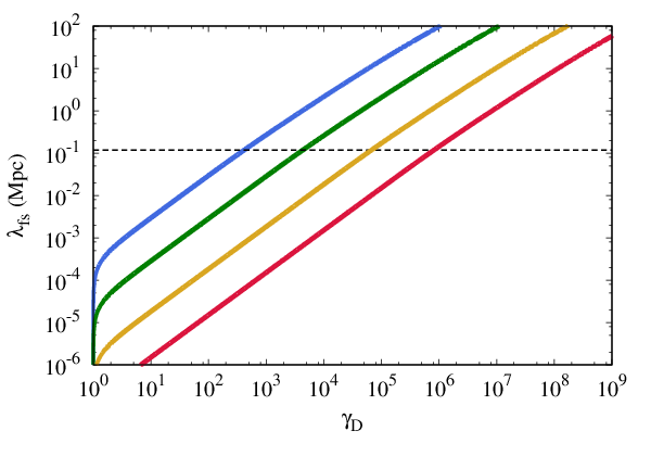
The above equation gives the scale at which the power spectrum of our model begins to differ from that of the standard $\Lambda$CDM power spectrum. Figure 7 shows the free-streaming length calculated by Eq. (IV.1) as a function of the Lorentz factor at decay, $\gamma_{D}$, for different values of the reheat temperature. We define $k_{\mathrm{fs}}=(\lambda_{\mathrm{fs},0}^{\mathrm{phys}})^{-1}$, and above the horizontal dashed line, the free-streaming length of the dark matter reaches scales probable by the Lyman-$\alpha$ forest: $k\lesssim 12.6\ h/\mathrm{Mpc},\lambda_{\mathrm{fs},0}^{\mathrm{phys}}\gtrsim 0.08\ \mathrm{Mpc}/h$. Since the free-streaming lengths of our model enter the observable regime, we consider a more precise determination of the effects of the dark matter free-streaming length in the next section.

We use the Cosmic Linear Anisotropy Solving System (CLASS) Lesgourgues and Tram 2015 to obtain the dark matter transfer function,

which describes suppression of structure due to non-cold dark matter (nCDM) compared to that of the standard CDM scenario; $P_{\mathrm{nCDM}}(k)$ and $P_{\mathrm{CDM}}(k)$ are the matter power spectra in each respective case.

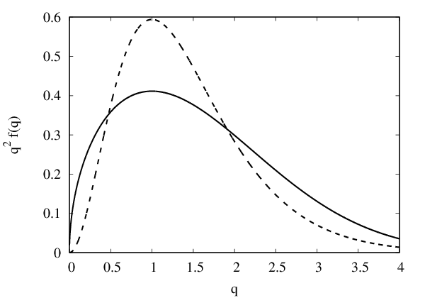
Acquiring the power spectrum for our scenario requires us to determine the momentum distribution function of our dark matter model. Shortly after reheating ($a\sim 3a_{\mathrm{RH}}$), the scalar field has decayed almost entirely, and essentially no new dark matter particles are being produced. After this point, the distribution of the comoving momenta of the dark matter particles does not change. We scale the comoving momenta of the dark matter particles by the comoving momentum of a particle born at the scale factor that maximizes $f(a_{D})$, $a_{\mathrm{max}}=0.68a_{\mathrm{RH}}$, and express our distribution function in terms of

where $p_{D}$ is the physical momentum of a particle with velocity $v_{D}$. Since we assume that all dark matter particles are produced with the same velocity, the distribution in momentum for particles in our scenario can be entirely determined from the distribution in the particles’ scale factor at production, which we have already determined. The two distribution functions can be related through

This distribution function is shown in Fig. 8, and we also show for comparison the Fermi-Dirac distribution that is maximized at $q=1$. We can see that, compared to the thermal case, we have a broader distribution function.

With our distribution function $f(q)$, we are able to use CLASS to obtain transfer functions for any combination of the velocity imparted to the dark matter and the reheat temperature by also providing the present-day physical momentum of a dark matter particle with $q=1$:

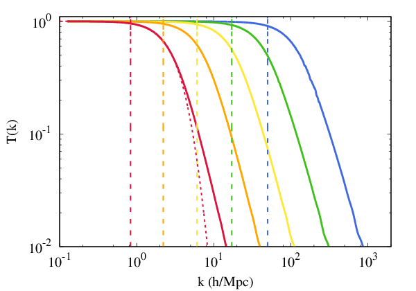
Again we find that, just as in our calculations of the free-streaming length, the relevant combination of parameters is $\mu=\gamma_{D}v_{D}a_{\mathrm{RH}}/a_{0}$. In Figs. 9 and 10 we show the transfer functions for dark matter produced at different velocities, but in scenarios with the same reheat temperature, 3 MeV. As expected, dark matter particles born at greater velocities result in the suppression of larger scales (smaller $k$). The vertical dashed lines in Fig. 9 mark the free-streaming horizon $k_{\mathrm{fs}}=(\lambda_{\mathrm{fs},0}^{\mathrm{phys}})^{-1}$ given by Eq. (IV.1) for each of the different velocities at production, confirming that it is the scale at which our model begins to show deviation, $T(k)\simeq 0.95$, from the CDM scenario.

Transfer functions in nCDM models, such as this, can be well described by a fitting formula Murgia et al. 2017:

Using Lyman-$\alpha$ data, the fitting parameters $\alpha,\beta$, and $\gamma$ can be constrained Murgia et al. 2017; Murgia et al. 2018, and the parameters of our model, $v_{D}$ and $T_{\mathrm{RH}}$, can be constrained as well. The typical scale of the suppression is set by $\alpha$, whereas the general shape is determined by $\beta$ and $\gamma$. When fitting our transfer function at values $T(k)>0.01$, the overall shape of our transfer function varies little across wide ranges of our parameter space, and $\beta$ and $\gamma$ can be expressed as functions of $\alpha$, as seen in Fig. 11. The cutoff parameter $\alpha$ is then our only free parameter, and it can be robustly constrained using Lyman-$\alpha$ data.

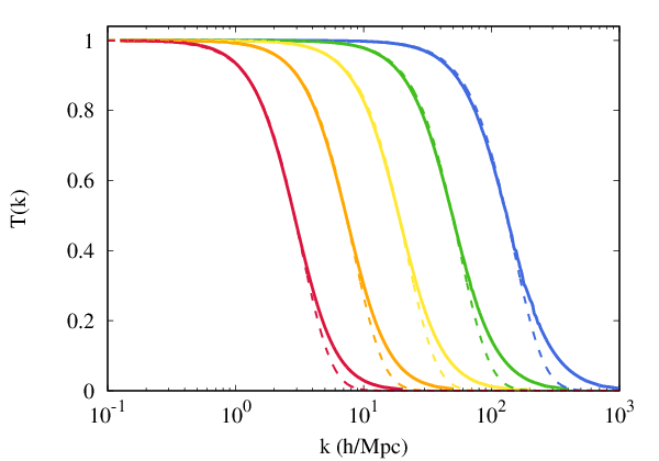
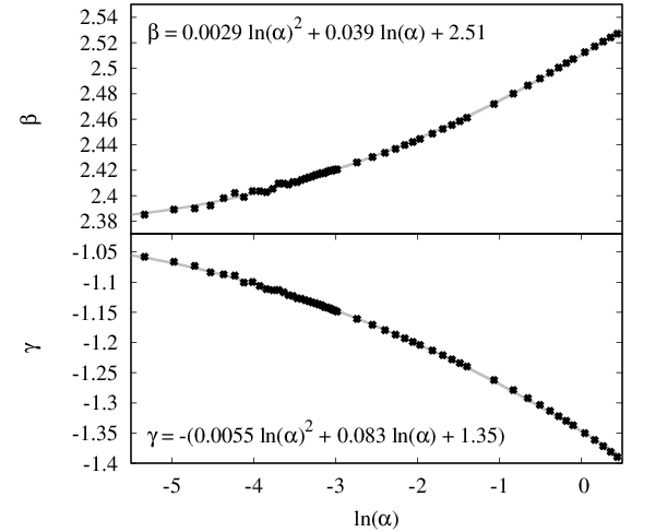
We find typical values of $\beta$ and $\gamma$ for our model to be approximately 2.4 and $-1.1$ respectively, for $\alpha$ near the constrainable regime. These values are noticeably different from those that describe the thermal warm dark matter (WDM) transfer function, $\beta_{\mathrm{WDM}}=2.24$ and $\gamma_{\mathrm{WDM}}=-4.46$. If we compare our transfer functions to those of WDM with the same value of the half-mode scale¹¹ 1 We follow the convention of Ref. Schneider et al. 2012 and define the half-mode scale via $T(k_{\mathrm{hm}})=0.5$, noting that this convention is different from the half-mode scale, $k_{1/2}$, defined in Refs. Murgia et al. 2017 and Murgia et al. 2018, for which $T^{2}(k_{1/2})=0.5$. $k_{\mathrm{hm}}$, we can see in Figs. 9 and 10 that the transfer functions in the two models are quite similar. However, due to the difference in the shape parameters of the transfer function fit between the two models, matching their half-mode scales requires the cutoff parameter in the WDM transfer function to be roughly a factor of $2$ smaller than that in the corresponding nonthermal transfer function, $\alpha\simeq 2\alpha_{\mathrm{WDM}}$. The cutoff in the transfer function of our model is not as sharp as that of WDM, but they only begin to differ significantly at scales at which the power in the nCDM model is already greatly suppressed, $T(k)\lesssim 0.1$.

Reference Murgia et al. 2018 provided marginalized bounds on all three fitting parameters in Eq. (34). The predictable shape of our transfer function determines the values of $\beta$ and $\gamma$ as a function of $\alpha$, as shown in Fig. 11, and allows us to obtain a bound on the remaining free parameter, the scale of the cutoff: $\alpha<0.011\mathrm{Mpc}/h$ (68% C.L.) and $\alpha<0.026\mathrm{Mpc}/h$ (95% C.L.). Following Ref. Murgia et al. 2018, these limits have been obtained by performing a comprehensive Markov hain Monte Carlo (MCMC) analysis of the full parameter space affecting the one-dimensional flux power spectrum, which is the Lyman-$\alpha$ forest physical observable, with a data set consisting of the high-resolution and high-redshift ($4.2<z<5.4$) quasar samples from MIKE and HIRES spectrographs Viel et al. 2013b. The flux power spectra to be compared against observations are estimated by interpolating in the multidimensional space defined by the sparse grid of precomputed hydrodynamic simulations described in Ref. Murgia et al. 2018. Whenever some of the parameters assume values not enclosed by the template of simulations, the corresponding values of the power spectra are linearly extrapolated.

As in the reference analysis from Ref. Murgia et al. 2018 (but see also, e.g., Refs. Archidiacono et al. 2019 and Murgia et al. 2019), the other cosmological and astrophysical parameters impacting our likelihood are treated as nuisance parameters to marginalize over. We adopt conservative flat priors on both $\sigma_{8}$, i.e. the normalization of the linear matter power spectrum, and $n_{\mathrm{eff}}$, i.e. the slope of the matter power spectrum at the scale of the Lyman-$\alpha$ forest ($k\sim 1h/$Mpc), in the intervals $[0.5,1.5]$ and $[-2.6,-2.0]$, respectively; and on the instantaneous reionization redshift $z_{\mathrm{reio}}$ (in the range $[7,15]$). Concerning the astrophysical parameters, we model the redshift evolution of the temperature of the intergalactic medium as a power law, imposing flat priors on both its amplitude and tilt (once again, see Ref. Murgia et al. 2018 for further details). Finally, we adopt conservative Gaussian priors on the mean Lyman-$\alpha$ forest fluxes $\langle F(z)\rangle$, with standard deviation $\sigma=0.04$ Iršič et al. 2017, and a flat prior on $f_{\mathrm{UV}}$, which is an effective parameter accounting for spatial ultraviolet fluctuations in the ionizing background.

Last but not least, we adopt a flat prior on $\alpha$ in the interval [0, 0.1] Mpc$/h$, while the parameters $\beta$ and $\gamma$ are derived analytically, per each MCMC step, according to the expressions reported in Fig. 11. For further details on the data set, simulations, and methods that we have used, we address the reader to any of the aforementioned references Murgia et al. 2018; Archidiacono et al. 2019; Murgia et al. 2019.

For comparison, just as matching the half-mode scale of the thermal WDM transfer function with that of our nonthermal model requires $\alpha\simeq 2\alpha_{\mathrm{WDM}}$, the $\alpha_{\mathrm{WDM}}$ value of a $3$ keV WDM particle, $\alpha_{\mathrm{WDM}}\simeq 0.015$ Mpc$/h$ Murgia et al. 2018, is approximately a factor of $2$ smaller than that of our 95% C.L. bound on $\alpha$. Our limits on $\gamma_{D}$ and $T_{\mathrm{RH}}$ corresponding to our 68% and 95% C.L. bounds on $\alpha$ are shown in Fig. 12. Scenarios in which the dark matter is born at too high of a velocity (large $\gamma_{D}$) or in which the radiation-dominated era is too short (low $T_{\mathrm{RH}}$) are part of the excluded parameter space for our relativistic nonthermal dark matter model. The thin grey lines represent contours of constant $f$, the fraction of the scalar’s energy imparted to the dark matter particle that is required to obtain the correct relic abundance for a given reheat temperature without dark matter annihilations. We can see that, in the absence of annihilations, the allowed values of $\gamma_{D}$ are not large enough for the required value of $f$ to be of order unity.

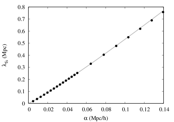
We also show the outline (dashed) of the parameter space in which the free-streaming length, calculated by Eq. (IV.1), is naively probable by Lyman-$\alpha$ data, i.e. $k_{\mathrm{fs}}<12.6h/\mathrm{Mpc}$. As can be seen in Fig. 12, limiting the free-streaming length provides a bound that is comparable to those obtained from the full consideration of effects to the matter power spectrum; the free-streaming scales of a particle on the boundary of our 68% and 95% C.L. regions are $k_{\mathrm{fs}}=11.4h/\mathrm{Mpc}$ and $28h/\mathrm{Mpc}$, respectively. While examining effects on the matter power spectrum leads to more robust bounds within our parameter space, calculations of the free-streaming length are more readily performed. Fortunately, as both the free-streaming length and the dark matter distribution function depend on the same combination of our parameters, $\gamma_{D}v_{D}a_{\mathrm{RH}}/a_{0}$, there is a simple relationship between the scale of suppression, $\alpha$, and the free-streaming length calculated by Eq. (IV.1):

We show this relationship in Fig. 13. In our model, the bounds on $\alpha$ can be easily used to limit the free-streaming length, and thereby the parameters $\gamma_{D}$ and $T_{\mathrm{RH}}$ on which it depends.

In addition to structures inferred by Lyman-$\alpha$ data, we can also constrain our model using observed structures in the Milky Way. Simulations of thermal warm dark matter provide an indication of how the suppression expected in the matter power spectrum decreases the abundance of collapsed objects. The subhalo mass function in simulations with WDM characterizes this underabundance Lovell et al. 2014,

where $M$ is the subhalo mass, $\delta=2.7$ and $\varepsilon=0.99$, and $M_{\mathrm{hm}}$ is the mass scale associated with the half-mode scale²² 2 We have verified with the authors of Ref. Lovell et al. 2014 that they used the same definition of $k_{\mathrm{hm}}$ that we have presented here.:

where $\Omega_{\mathrm{DM}}$ is the fraction of the critical density in dark matter.

Knowing the abundance of satellites of our own galaxy, constraints can be placed on the amount of allowed suppression in the subhalo mass function. Using a probabilistic analysis of the MW satellite population and marginalizing over astrophysical uncertainties, Ref. Nadler et al. 2019 found an upper limit on $M_{\mathrm{hm}}$ in Eq. (36), $M_{\mathrm{hm}}<3.1\times 10^{8}M_{\odot}$ (95% C.L.), which implies that the half-mode scale must satisfy $k_{\mathrm{hm}}>36h/\mathrm{Mpc}$. This bound on $k_{\mathrm{hm}}$ can be used to constrain any dark matter model that has a transfer function comparable to WDM, as we have shown ours to be in Fig. 10. Though the transfer function of our model does differ slightly from that of WDM, the differences occur only when the nCDM power spectrum is already greatly suppressed compared to that of CDM, $T(k)\lesssim 0.1$. The fitting form to our transfer function, Eq. (34), implies that the half-mode scale is given by:

and the constraint $k_{\mathrm{hm}}>36\ h/$Mpc directly translates to $\alpha<0.026\ \mathrm{Mpc}/h$, matching our 95% C.L. bound from Lyman-$\alpha$ constraints.